Identifying graphene layers via spin Hall effect of light

Abstract

The spin Hall effect (SHE) of light is a useful metrological tool for characterizing the structure parameters variations of nanostructure. In this letter we propose using the SHE of light to identify the graphene layers. This technique is based on the mechanism that the transverse displacements in SHE of light are sensitive to the variations of graphene layer numbers.

The quick and convenient technique for identifying the layer numbers of graphene film is important for accelerating the study and exploration of graphene material Geim2009 . There have many methods for determining the layer numbers of graphene film, yet existing limitation. For instance, atomic force microscopy technique is the straight way to determine the layer numbers of graphene. But this method shows a slow throughput and may induce damage to the sample. Unconventional quantum Hall effects Zhang2005 are usually used to distinguish one layer and two layers graphene from multiple layers. Raman spectroscopy Gupta2006 shows characteristic for quick and nondestructive measuring the layer numbers of graphene. However, it is not obvious to tell the differences between bilayer and a few layers of graphene films Ni2007 .

The spin Hall effect (SHE) of light appears as a transverse spin-dependent splitting, when a spatially confined light beam passes from one material to another with different refractive index Onoda2004 ; Bliokh2006 ; Gorodetski2008 ; Luo2011a ; Bliokh2008 ; Hosten2008 ; Qin2009 ; Aiello2008 ; Hermosa2011 ; Menard2009 . The SHE of light is the photonic version of the spin Hall effect in electronic systems, in which the spin photons play the role of the spin charges, and a refractive index gradient plays the role of the electric potential gradient. The SHE of light holds great potential applications, such as manipulating electron spin states and precision metrology. Importantly, the SHE of light can serve as a useful metrological tool for characterizing the structure parameters variations of nanostructure due to their sensitive dependence Hosten2008 . For example, in the previous work, we have measured the thickness of the nanometal film via weak measurements Zhou2012a . Therefore the SHE of light may have a potential to determine the layer numbers of graphene.

Figure 1: (Color online) Schematic of SHE of light on a graphene film. A linearly polarized beam reflects on the model and then splits into left- and right-circularly polarized light, respectively. $\delta_{+}$ and $\delta_{-}$ indicate the transverse shift of left- and right-circularly polarized components. Here, $\theta_{i}$ is the incident angle and the inset shows the atomic structure of graphene.

In this letter, we propose a simple method for measuring the layer numbers of graphene. We find that SHE of light can serve as an advantageous metrology tool for characterizing the layer numbers of graphene. The rest of the paper is organized as follows. First a general propagation model is used to analyze the SHE of light on a graphene film. We establish the relationship between the transverse shifts and the graphene layers. Then, we focus our attention on the experiment for judging the layer numbers of graphene. Here we use the SHE of light to choose the suitable refractive index of graphene obtaining from the literature. And then, with the suitable refractive index, the layer numbers of an unknown graphene film can be detected. We introduce the weak measurements technique and the sample is a BK7 substrate transferred with the graphene film using the chemical vapor deposited (CVD) method. Finally, we summarize the main results of the paper.

We first theoretically analyze the SHE of light on graphene film and establish the relationship between transverse shifts and the layer numbers of graphene. Figure 1 schematically illustrates the SHE of light reflection on a graphene film in Cartesian coordinate system. The $z$ axis of the laboratory Cartesian frame ($x,y,z$) is normal to the interface of the graphene film at $z=0$. The incident and reflected electric fields are presented in coordinate frames ($x_{i},y_{i},z_{i}$) and ($x_{r},y_{r},z_{r}$), respectively. In the spin basis set, the angular spectrum can be written as $\tilde{\mathbf{E}}_{i}^{H}=(\tilde{\mathbf{E}}_{i+}+\tilde{\mathbf{E}}_{i-})/{\sqrt{2}}$ and $\tilde{\mathbf{E}}_{i}^{V}=i(\tilde{\mathbf{E}}_{i-}-\tilde{\mathbf{E}}_{i+})/{\sqrt{2}}$. Here, $H$ and $V$ represent horizontal and vertical polarizations, respectively. The positive and negative signs represent the left- and right-circularly polarized (spin) components, respectively.

The incident monochromatic Gaussian beam can be formulated as a localized wave packet whose spectrum is arbitrarily narrow, and can be written as

$$\widetilde{\mathbf{E}}_{i\pm}=(\mathbf{e}_{ix}+i\sigma\mathbf{e}_{iy})\frac{w_{0}}{\sqrt{2\pi}}\exp\left[-\frac{w_{0}^{2}(k_{ix}^{2}+k_{iy}^{2})}{4}\right],$$ (1)

where $w_{0}$ is the beam waist. The polarization operator $\sigma=\pm 1$ corresponds to left- and right-circularly polarized light, respectively. In this work, we only consider the incident light beam with horizontal polarization and vertical polarization can be analyzed in the similar way. Using the reflection matrix Luo2011b ; Zhou2012b , we can obtain the expressions of the reflected angular spectrum

$$\widetilde{\mathbf{E}}_{r}=\frac{r_{p}}{\sqrt{2}}\left[\exp(+ik_{ry}\delta_{r})\widetilde{\mathbf{E}}_{r+}+\exp(-ik_{ry}\delta_{r})\widetilde{\mathbf{E}}_{r-}\right].$$ (2)

Here, $\delta_{r}=(1+r_{s}/r_{p})\cot\theta_{i}/k_{0}$, $r_{p}$ and $r_{s}$ denote Fresnel reflection coefficients for parallel and perpendicular polarizations, respectively. $k_{0}$ is the wave number in free space. And the $\widetilde{\mathbf{E}}_{r\pm}$ can be written as

$$\widetilde{\mathbf{E}}_{r\pm}=(\mathbf{e}_{rx}+i\sigma\mathbf{e}_{ry})\frac{w_{0}}{\sqrt{2\pi}}\exp\left[-\frac{w_{0}^{2}(k_{rx}^{2}+k_{ry}^{2})}{4}\right].$$ (3)

At any given plane $z_{r}=const.$, the transverse displacement of field centroid compared to the geometrical-optics prediction is given by

$$\delta_{\pm}=\frac{\int\int\tilde{\mathbf{\xi}}^{\ast}_{r\pm}i\partial_{k_{ry}}\tilde{\mathbf{\xi}}_{r\pm}dk_{rx}dk_{ry}}{\int\int\tilde{\mathbf{\xi}}^{\ast}_{r\pm}\tilde{\mathbf{\xi}}_{r\pm}dk_{rx}dk_{ry}},$$ (4)

where $\tilde{\mathbf{\xi}_{r}}_{\pm}$ = $r_{p}\exp(\pm ik_{ry}\delta_{r})\widetilde{\mathbf{E}}_{r\pm}$. Calculating the reflected displacements of the SHE of light requires the explicit solution of the boundary conditions at the interfaces. Thus, we need to know the generalized Fresnel reflection of the graphene film,

$$r_{A}=\frac{R_{A}+R_{A}^{{}^{\prime}}\exp(2ik_{0}\sqrt{n^{2}-\sin^{2}\theta_{i}}d)}{1+R_{A}R_{A}^{{}^{\prime}}\exp(2ik_{0}\sqrt{n^{2}-\sin^{2}\theta_{i}}d)}.$$ (5)

Here, $A\in\{p,s\}$, $R_{A}$ and $R_{A}^{{}^{\prime}}$ is the Fresnel reflection coefficients at the first interface and second interface, respectively. $n$ and $d$ represent the refractive index and thickness of the graphene film, respectively. The thickness of the graphene film is about $d=m\Delta d$ in which $m$ denotes the layer numbers and $\Delta d$ represents the thickness of single layer graphene ($\Delta d$ is about $0.34$ nm). So far we have established the relationship between the transverse shifts and the graphene layers. After obtaining the displacements of SHE of light, we can determine the layer numbers of graphene.

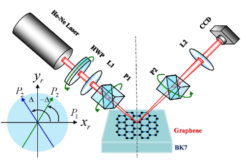
Figure 2: (Color online) Experimental setup: The sample is a BK7 glass transferred with the graphene film. L1 and L2, lenses with effective focal length $50$ mm and $250$ mm, respectively. HWP, half-wave plate (for adjusting the intensity). P1 and P2, Glan Laser polarizers. CCD, charge-coupled device (Coherent LaserCam HR). The light source is a $17$ mW linearly polarized He-Ne laser at $633$ nm (Thorlabs HRP170). The inset shows that the angle between P1 and P2 is $90^{\circ}\pm\Delta$.

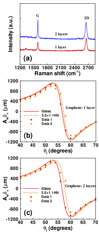
Figure 3: (Color online) Raman spectra of the samples and the graphene refractive index selection in the case of horizontal polarization. (a) Raman spectra of one, two graphene layers. (b) represents the transverse displacements under the condition of single layer graphene. We choose the thickness of one layer graphene film as 0.34 nm. The transverse shifts in the case of two layers graphene film are shown in (c). Here, the lines represent the theoretical results. The circle and triangle show the experimental results obtained from the air-prism and different graphene-prism condition via weak measurements. The refractive index of the BK7 substrate is chosen as $n=1.515$ at $633$ nm.

In this work a signal enhancement technique known as the weak measurements Aharonov1988 ; Ritchie1991 is used to measure the tiny transverse displacements. The experimental setup shown in Fig. 2 is similar to that in Refs Luo2011a ; Qin2009 . A Gaussian beam generated by a He-Ne laser passes through a short focal length lens (L1) and a polarizer (P1) to produce an initially horizontal polarization beam. Here the half-wave plate (HWP) is used to control the light intensity. When the beam impinges onto the graphene-prism interface, the SHE of light takes place, manifesting itself as the opposite displacements of the two spin components. Then the two components interfere destructively after the second polarizer (P2) which is oblique to P1 with an angle of $90^{\circ}\pm\Delta$. We note that the incident light beam is preselected in the H polarization state by P1 (along to the $x_{i}$-axis) and then postselected by P2 in the polarization state with $\mathbf{V}=\sin\Delta\mathbf{e}_{rx}+\cos\Delta\mathbf{e}_{ry}$. In this condition, we choose the angle $\Delta=2^{\circ}$. Then we use L2 to collimate the beam and make the beam shifts insensitive to the distance between L2 and the CCD. The reflected field at the plane of $z_{r}$ can be obtained with $\mathbf{V}\cdot\mathbf{E}_{r}$. The amplified displacement $\delta_{w}$ at the CCD is much larger than the initial shift $|\delta_{\pm}|$. Calculating the distribution of $\mathbf{V}\cdot\mathbf{E}_{r}$ yields the amplified factor $A_{w}=\delta_{w}/\delta_{+}$. Hence the amplified displacements at the CCD are $A_{w}\delta_{\pm}$. It should be mentioned that the amplified factor $A_{w}$ is not a constant, which verifies the similar result of our previous work Luo2011a .

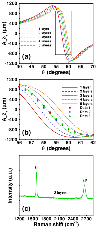
Figure 4: (Color online) The theoretical and experimental results of determining the layer numbers of graphene. (a) represents the theoretical transverse displacements under the condition of graphene layer numbers changing from one to five. Here the refractive index of graphene is $3.0+1.149i$ at $633$ nm. (b) describes the transverse shifts in the case of different incident angles ranging from $56^{\circ}$ to $62^{\circ}$. The lines represent the theoretical results. The circle, square and triangle show the experimental data obtained from three different areas of the graphene sample. (c) Raman reference data of the sample.

Now we focus our attention on identifying graphene layers. However, there exists two unknown parameters (refractive index and layer numbers of graphene) to be identified. Before identifying the graphene layers, we need to choose the suitable refractive index parameter of graphene. There has several measured values of the refractive index of graphene reported recently Blake2007 ; Ni2007 ; Wang2008 ; Bruna2009 . Here we choose one suitable refractive index according from the work of Bruna and Borini Bruna2009 . They concluded that the refractive index of graphene in the visible range consists of real refractive index (constant) and complex refractive index (depending on the wavelength). Here the refractive index of graphene is about $3.0+1.149i$ at 633 nm. We first need to prove that this refractive index is suitable for our graphene film. Our sample consists of graphene films with two different layers: one layer, two layers. The graphene films (made from ACS Material company) were first grown on $25{\mu}m$ thick copper foil in a quartz tube furnace system using a CVD method and then were transferred to the prism. The Raman spectra of these two samples are shown in Fig. 3(a). We measure the displacements of the SHE of light on the graphene film every $2^{\circ}$ from $40^{\circ}$ to $70^{\circ}$ in the case of horizontal polarization and the results are shown in Fig. 3(b) and 3(c). It should be noted that the quality of the material (graphene film) and the experimental environment will affect the measurement. A group of experiment for measuring the SHE of light at a pure air-prism interface was also carried out for making a reference. We can find that the experimental results fit well with the transverse displacement curve calculated from the literature of Bruna Bruna2009 . We can obtain that the refractive index of graphene is really close to $3.0+1.149i$ at $633$ nm. Therefore the SHE of light provides us an alternative way for choosing the refractive index of graphene.

Using the suitable refractive index $n=3.0+1.149i$ at $633$ nm, we can identify the layer numbers of an unknown graphene film with the weak measurements. The experimental sample is also prepared with the CVD method. It should be noted that, in our experimental condition, we can not fabricate the sample with the precise layer numbers when the graphene film has more than two layers. Because it would unavoidably involve large technical errors. We just know the approximate layer numbers ranges. Therefore we prepare a sample with the possible layer numbers ranging from three to five layers. Our aim is to determine the actual layer numbers of this graphene film. Figure 4 shows the theoretical and experimental results of the graphene layer numbers determination. From Fig. 4(a), we find that it is hard to distinguish the transverse shifts of the different graphene layer numbers from $40^{\circ}$ to $70^{\circ}$. Thence we measure the transverse displacements in a small range of incident angle (from $56^{\circ}$ to $62^{\circ}$) to obtain a desired results [Fig. 4(b)]. To avoid the influence of impurities and other surface quality factors of graphene film, we carried out the experiments for three different areas of the graphene sample. From the experimental results, we can conclude that the actual layer numbers of the film is three. To further confirm our results, we also add some reference data via measuring the Raman spectra of the sample as shown in Fig. 4(c). Therefore the SHE of light can become a useful metrological tool for characterizing the layer numbers of graphene.

In conclusion, we have presented a simple and convenient method for determining the layer numbers of graphene. Firstly, we use the SHE of light to choose the suitable refractive index of graphene obtaining from the corresponding literature. And then, with the suitable refractive index $n=3.0+1.149i$ at $633$ nm, the layer numbers of an unknown graphene film can be detected with desired precise. So combining the SHE of light with the other techniques such as atomic force microscopy and Raman spectroscopy can improve the graphene layers identification accuracy, which is important for the future graphene research.

One of the authors (X. Z.) would like to thank Dr. Sosan Cheon for helpful discussions. This research was partially supported by the National Natural Science Foundation of China (Grants Nos. 61025024 and 11274106) and Hunan Provincial Natural Science Foundation of China (Grant No. 12JJ7005).

References

- (1) A. K. Geim, Science 324, 1530 (2009).
- (2) Y. B. Zhang, Y. W.Tan, H. L. Stormer, and P. Kim, Nature 438, 201 (2005).
- (3) A. Gupta, G. Chen, P. Joshi, S. Tadigadapa, and P. C. Eklund, Nano Lett. 6, 2667 (2006).
- (4) Z. H. Ni, H. M. Wang, J. Kasim, H. M. Fan, T. Yu, Y. H. Wu, Y. P. Feng, and Z. X. Shen, Nano Lett. 7, 2758 (2007).
- (5) M. Onoda, S. Murakami, and N. Nagaosa, Phys. Rev. Lett. 93, 083901 (2004).
- (6) K. Y. Bliokh and Y. P. Bliokh, Phys. Rev. Lett. 96, 073903 (2006).
- (7) Y. Gorodetski, A. Niv, V. Kleiner, and E. Hasman, Phys. Rev. Lett. 101, 043903 (2008).
- (8) H. Luo, X. Zhou, W. Shu, S. Wen, and D. Fan, Phys. Rev. A 84, 043806 (2011).
- (9) K. Y. Bliokh, A. Niv, V. Kleiner, and E. Hasman, Nature Photon. 2, 748 (2008).
- (10) O. Hosten and P. Kwiat, Science 319, 787 (2008).
- (11) Y. Qin, Y. Li, H. He, and Q. Gong, Opt. Lett. 34, 2551 (2009).
- (12) A. Aiello and J. P. Woerdman, Opt. Lett. 33, 1437 (2008).
- (13) N. Hermosa, A. M. Nugrowati, A. Aiello, and J. P. Woerdman, Opt. Lett. 36, 3200 (2011).
- (14) J.-M. Ménard, A. E. Mattacchione, M. Betz, and H. M. van Driel, Opt. Lett. 34, 2312 (2009).
- (15) X. Zhou, Z. Xiao, H. Luo, and S. Wen, Phys. Rev. A 85, 043809 (2012).
- (16) H. Luo, X. Ling, X. Zhou, W. Shu, S. Wen, and D. Fan, Phys. Rev. A 84, 033801 (2011).
- (17) X. Zhou, H. Luo, and S. Wen, Opt. Express 20, 16003 (2012).
- (18) Y. Aharonov, D. Z. Albert, and L. Vaidman, Phys. Rev. Lett. 60, 1351 (1988).
- (19) N. W. M. Ritchie, J. G. Story, and R. G. Hulet, Phys. Rev. Lett. 66, 1107 (1991).
- (20) P. Blake, E. W. Hill, A. H. Castro Neto, K. S. Novoselov, D. Jiang, R. Yang, T. J. Booth, and A. K. Geim, Appl. Phys. Lett. 91, 063124 (2007).
- (21) Xuefeng Wang, Yong P. Chen and David D. Nolte, Opt. Express 16, 22105 (2008).
- (22) M. Bruna and S. Borini, Appl. Phys. Lett. 94, 031901 (2009).