Superiorization: An optimization heuristic for medical physics

Abstract

Purpose: To describe and mathematically validate the superiorization methodology, which is a recently-developed heuristic approach to optimization, and to discuss its applicability to medical physics problem formulations that specify the desired solution (of physically given or otherwise obtained constraints) by an optimization criterion.

Methods: The superiorization methodology is presented as a heuristic solver for a large class of constrained optimization problems. The constraints come from the desire to produce a solution that is constraints-compatible, in the sense of meeting requirements provided by physically or otherwise obtained constraints. The underlying idea is that many iterative algorithms for finding such a solution are perturbation resilient in the sense that, even if certain kinds of changes are made at the end of each iterative step, the algorithm still produces a constraints-compatible solution. This property is exploited by using permitted changes to steer the algorithm to a solution that is not only constraints-compatible, but is also desirable according to a specified optimization criterion. The approach is very general, it is applicable to many iterative procedures and optimization criteria used in medical physics.

Results: The main practical contribution is a procedure for automatically producing from any given iterative algorithm its superiorized version, which will supply solutions that are superior according to a given optimization criterion. It is shown that if the original iterative algorithm satisfies certain mathematical conditions, then the output of its superiorized version is guaranteed to be as constraints-compatible as the output of the original algorithm, but it is superior to the latter according to the optimization criterion. This intuitive description is made precise in the paper and the stated claims are rigorously proved. Superiorization is illustrated on simulated computerized tomography data of a head cross-section and, in spite of its generality, superiorization is shown to be competitive to an optimization algorithm that is specifically designed to minimize total variation.

Conclusions: The range of applicability of superiorization to constrained optimization problems is very large. Its major utility is in the automatic nature of producing a superiorization algorithm from an algorithm aimed at only constraints-compatibility; while non-heuristic (exact) approaches need to be redesigned for a new optimization criterion. Thus superiorization provides a quick route to algorithms for the practical solution of constrained optimization problems.

I Introduction

Optimization is a tool that is used in many areas of Medical Physics. Prime examples are radiation therapy treatment planning and tomographic reconstruction, but there are others such as image registration. Some well-cited classical publications on the topic are DEAS97a (1, 2, 3, 4, 5, 6, 7, 8, 9, 10, 11, 12) and some recent articles are ABDO10a (13, 14, 15, 16, 17, 18, 19, 20, 21, 22, 23, 24, 25, 26).

In a typical medical physics application, one uses constrained optimization, where the constraints come from the desire to produce a solution that is constraints-compatible, in the sense of meeting the requirements provided by physically or otherwise obtained constraints. In radiation therapy treatment planning, the requirements are usually in the form of constraints prescribed by the treatment planner on the doses to be delivered at specific locations in the body. These doses in turn depend on information provided by an imaging instrument, typically a Magnetic Resonance Imaging (MRI) or a Computerized Tomography (CT) scanner. In tomography, the constraints come from the detector readings of the instrument. In such applications, it is typically the case that a large number of solutions would be considered good enough from the point of view of being constraints-compatible; to a large extent, but not entirely, due to the fact that there is uncertainty as to the exact nature of the constraints (for example, due to noise in the data collection). In such a case, an optimization criterion is introduced that helps us to distinguish the “better” constraints-compatible solutions (for example, this criterion could be the total dose to be delivered to the body, which may vary quite a bit between radiation therapy treatment plans that are compatible with the constraints on the doses delivered to individual locations).

The superiorization methodology (see, for example, PENF10a (22, 29, 28, 30, 31, 27, 32)) is a recently-developed heuristic approach to optimization. The word heuristic is used here in the sense that the process is not guaranteed to lead to an optimum according to the given criterion; approaches aimed at processes that are guaranteed in that sense are usually referred to as exact. Heuristic approaches have been found useful in practical applications of optimization, mainly because they are often computationally much less expensive than their exact counterparts, but nevertheless provide solutions that are appropriate for the application at hand RARD01a (33, 34, 35).

The underlying idea of the superiorization approach is the following. In many applications there exists a computationally-efficient iterative algorithm that produces a constraints-compatible solution for the given constraints. (An example of this for radiation therapy treatment planning is reported in Herman2008 (36), its clinical use is discussed in CHEN10a (15).) Furthermore, often the algorithm is perturbation resilient in the sense that, even if certain kinds of changes are made at the end of each iterative step, the algorithm still produces a constraints-compatible solution CENS10a (29, 28, 30, 27). This property is exploited in the superiorization approach by using such perturbations to steer the algorithm to a solution that is not only constraints-compatible, but is also desirable according to a specified optimization criterion. The approach is very general, it is applicable to many iterative procedures and optimization criteria.

The current paper presents a major advance in the practice and theory of superiorization. The previous publicationsPENF10a (22, 29, 28, 30, 31, 27, 32) used the intuitive idea to present some superiorization algorithms, in this paper the reader will find a totally automatic procedure that turns an iterative algorithm into its superiorized version. This version will produce an output that is as constraints-compatible as the output of the original algorithm, but it is superior to that according to an optimization criterion. This claim is mathematically shown to be true for a very large class of iterative algorithms and for optimization criteria in general, typical restrictions (such as convexity) on the optimization criterion are not essential for the material presented below. In order to make precise and validate this broad claim, we present here a new theoretical framework. The framework of CENS10a (29) is a precursor of what we present here, but it is a restricted one, since it assumes that the constraints can be all satisfied simultaneously, which is often false in medical physics applications. There is no such restriction in the presentation below.

The idea of designing algorithms that use interlacing steps of two different kinds (in our case, one kind of steps aim at constraints-compatibility and the other kind of steps aim at improvement of the optimization criterion) is well-established and, in fact, is made use of in many approaches that have been proposed with exact constrained optimization in mind; see, for example, the works of Helou Neto and De Pierrohdp-siam09 (37, 38), of Nurminskinur10 (39), of Combettes and coworkersCOMB02a (40, 41), of Sidky and Pan and coworkersSIDK11a (23, 42, 43) and of Defrise and coworkersDEFR11a (44). However, none of these approaches can do what can be done by the superiorization approach as presented below, namely the automatic production of a heuristic constrained optimization algorithm from an iterative algorithm for constraints-compatibility. For example, in hdp-siam09 (37) it is assumed (just as in the theory presented in our CENS10a (29)) that all the constraints can be satisfied simultaneously.

A major motivator for the additional theory presented in the current paper is to get rid of this assumption, which is not reasonable when handling real problems of medical physics. Motivated by similar considerations, Helou Neto and De Pierro hdp11 (38) present an alternative approach that does not require this unreasonable assumption. However, in order to solve such a problem, they end up with iterative algorithms of a particular form rather than having the generality of being able to turn any constraints-compatibility seeking algorithm into a superiorized one capable of handling constrained optimization. Also, the assumptions they have to make in order to prove their convergence result (their Theorem 15) indicate that their approach is applicable to a smaller class of constrained optimization problems than the superiorization approach whose applicability seems to be more general. However, for the mathematical purist, we point out that they present an exact constrained optimization algorithm, while superiorization is a heuristic approach. Whether this is relevant to medical physics practice is not clear: exact algorithms are not run forever, but are stopped according to some stopping-rule, the relevant questions in comparing two algorithms are the quality of the actual output and the computation time needed to obtain it.

Ultimately, the quality of the outputs should be evaluated by some figures of merit relevant to the medical task at hand. An example of a careful study of this kind that involves superiorization is in (NIKA12a, 30, Section 4.3), which reports on comparing in CT the efficacy of constrained optimization reconstruction algorithms for the detection of low-contrast brain tumors by using the method of statistical hypothesis testing (which provides a P-value that indicates the significance by which we can reject the null hypothesis that the two algorithms are equally efficacious in favor of the alternative that one is preferable). Such studies bundle together two things: (i) the formulation of the constrained optimization task and (ii) the performance of the algorithm in performing that task. The first of these requires a translation of the medical aim into a mathematical model, it is important that this model should be appropriately chosen.

The superiorization approach is not about choosing this model, it kicks in once the model is chosen and aims at producing an output that is “good” according to the mathematical specifications of the constraints and of the optimization criterion. Thus superiorization has been used to compare the effects on the quality of the output in CT when the optimization criterion is specified by total variation (TV) versus by entropyDAVI09a (28) or versus by the $\ell_{1}$-norm of the Haar transform GARD11a (32). However, the current paper is not about discussing how to translate the underlying medical physics task into a constrained optimization problem. For our purposes here, we are assuming that the mathematical model has been worked out and concentrate on the algorithmic approach for solving the resulting constrained optimization problem. We claim that the evaluation of such algorithms should not be based on the medical figures of merit mentioned at the beginning of the previous paragraph, but rather on their performance in solving the mathematical problem. If “good” solutions to the constrained optimization problem are not medically efficacious, that indicates that something is wrong with the mathematical model and not that something is wrong with the algorithmic approach. For this reason, in this paper we will not carry out a careful investigation of the medical efficacy of any algorithm in the manner that we have done in (NIKA12a, 30, Section 4.3), but will restrict ourselves to a simple illustration of the performance of the superiorization approach as compared to the previously published algorithm ofSIDK08a (42) that is aimed at performing exact minimization.

Examples of such studies already exist. Superiorization was compared in BUTN07a (27) with Algorithm 6 of COMB02a (40) and in CENS12a (45) with the algorithm of Goldstein and Osher that they refer to as TwIST BIOU07a (46) with split Bregman GOLD09a (47) as the substep. In both cases the implementation was done by the proposers of the algorithms. In these reported instances superiorization did well: the constraints-compatibility and the value of the function to be minimized were very similar for the outputs produced by the algorithms being compared, but the superiorization algorithm produced its output four times faster than the alternative. It would be unjustified to draw any general conclusions on the mathematical performance and speed of superiorization based on just a few experiments, but the reported results are encouraging.

However, the main reason why we advocate superiorization is different from what is discussed above. The reason why we claim it to be helpful in medical physics research is that it has the potential of saving a lot of time and effort for the researcher. Let us consider a historical example. Likelihood optimization using the iterative process of expectation maximization (EM) SHEP82a (48) gained immediate and wide acceptance in the emission tomography community. It was observed that irregular high amplitude patterns occurred in the image with a large number of iterations, but it was not until five years later that this problem was corrected LEVI87A (49) by the use of a maximum a posteriority probability (MAP) algorithm with a multivariate Gaussian prior. Had we had at our disposal the superiorization approach, then the introduction of an optimization criterion (Gaussian or other) into the iterative expectation maximization (EM) process would have been a simple matter and we would have saved the time and effort spent on designing a special purpose algorithm for the MAP formulation. A $TV$-superiorization of the EM algorithm is presented inJIN12a (50).

Even though our major claim for superiorization is that it provides a quick route to algorithms for the practical solution of constrained optimization problems, before leaving this introduction let us bring up a question that has to do with the performance of the resulting algorithms: Will superiorization produce superior results to those produced by contemporary MAP methods or is it faster than the better of such methods? At this stage we have not yet developed the mathematical notation to discuss this question in a rigorous manner, we return to it in Subsection II.6.

In the next section we present in detail the superiorization methodology. In the subsequent section we provide an illustrative example by reporting on reconstructions produced by algorithms applied to simulated computerized tomography data of a head cross-section. In the final section we discuss our results and present our conclusions.

II The Superiorization Methodology

II.1 Problem sets, proximity functions and $\varepsilon$-compatibility

Although optimization is often studied in a more general context (such as in Hilbert or Banach spaces), in medical physics we usually deal with a special case, where optimization is performed in a Euclidean space $\mathbb{R}^{J}$ (the space of $J$-dimensional vectors of real numbers, where $J$ is a positive integer). As often appropriate in practice, we further restrict the domain of optimization to a nonempty subset $\Omega$ of $\mathbb{R}^{J}$ (such as the nonnegative orthant $\mathbb{R}_{+}^{J}$ that consists of vectors all of whose components are nonnegative).

We now turn to formalizing the notion of being compatible with given constraints, a notion that we have used informally in the previous section. In any application, there is a problem set $\mathbb{T}$; each problem $T\in\mathbb{T}$ is essentially a description of the constraints in that particular case. For example, for a tomographic scanner, the problem of reconstruction for a particular patient at a particular time is determined by the measurements taken by the scanner for that patient at that time. The intuitive notion of constraints-compatibility is formalized by the use of a proximity function $\mathcal{P}r$ on $\mathbb{T}$ such that, for every $T\in\mathbb{T}$, $\mathcal{P}r_{T}$ maps $\Omega$ into $\mathbb{R}_{+}$, the set of nonnegative real numbers; i.e., $\mathcal{P}r_{T}:\Omega\rightarrow\mathbb{R}_{+}$. Intuitively we think of $\mathcal{P}r_{T}\left(\boldsymbol{x}\right)$ as an indicator of how incompatible $\boldsymbol{x}$ is with the constraints of $T$. For example, in tomography, $\mathcal{P}r_{T}\left(\boldsymbol{x}\right)$ should indicate by how much a proposed reconstruction that is described by an $\boldsymbol{x}$ in $\Omega$ violates the constraints of the problem $T$ that are provided by the measurements taken by the scanner. For example, if we use $\boldsymbol{b}$ to denote the vector of estimated line integrals based on the measurements obtained by the scanner and by $\boldsymbol{A}$ the system matrix of the scanner, then a possible choice for the proximity function is the norm-distance $\left\|\boldsymbol{b-Ax}\right\|$, which we will use as an example in the discussions that follow. An alternative legitimate choice for the proximity function is the Kullback-Leibler distance $KL(\boldsymbol{b},\boldsymbol{Ax})$, which is the negative log-likelihood of a statistical model in tomography. The special case $\mathcal{P}r_{T}\left(\boldsymbol{x}\right)=0$ is interpreted by saying that $\boldsymbol{x}$ is perfectly compatible with the constraints; due to the presence of noise in practical applications, it is quite conceivable that there is no $\boldsymbol{x}$ that is perfectly compatible with the constraints, and we accept an $\boldsymbol{x}$ as constraints-compatible as long as the value of $\mathcal{P}r_{T}\left(\boldsymbol{x}\right)$ is considered to be small enough to justify that decision. Combining these two concepts leads to the notion of a problem structure, which is a pair $\left\langle\mathbb{T},\mathcal{P}r\right\rangle$, where $\mathbb{T}$ is a nonempty problem set and $\mathcal{P}r$ is a proximity function on $\mathbb{T}$. For a problem structure $\left\langle\mathbb{T},\mathcal{P}r\right\rangle$, a problem $T\in\mathbb{T}$, a nonnegative $\varepsilon$ and an $\boldsymbol{x}\in\Omega$, we say that $\boldsymbol{x}$ is $\varepsilon$-compatible with $T$ provided that $\mathcal{P}r_{T}\left(\boldsymbol{x}\right)\leq\varepsilon$.

As an example (whose applicability to tomographic reconstruction is illustrated in Section III), consider the problem structure that arises from the desire to find nonnegative solutions of sequences of blocks of linear equations. Then the appropriate choices are $\Omega=\mathbb{R}_{+}^{J}$ and the problem structure is $\left\langle\mathbb{S},Res\right\rangle$, where the problem set $\mathbb{S}$ is

$$\begin{array}[]{lll}\mathbb{S}&=&\left\{\left(\left\{\left(\boldsymbol{a}^{1},b_{1}\right),\ldots,\left(\boldsymbol{a}^{\ell_{1}},b_{\ell_{1}}\right)\right\},\ldots,\right.\right.\\ &&\left.\left.\left\{\left(\boldsymbol{a}^{\ell_{1}+\ldots+\ell_{W-1}+1},b_{\ell_{1}+\ldots+\ell_{W-1}+1}\right),\ldots,\left(\boldsymbol{a}^{\ell_{1}+\ldots+\ell_{W}},b_{\ell_{1}+\ldots+\ell_{W}}\right)\right\}\right)\right|\\ &&W\mbox{ is a positive integer and,}\\ &&\mbox{for $1\leq w\leq W,\;\ell_{w}\>$is a positive integer and,}\\ &&\left.\mbox{for }1\leq i\leq\ell_{1}+\ldots+\ell_{W},\>\boldsymbol{a}^{i}\in\mathbb{R}^{J}\mbox{ and }b_{i}\in\mathbb{R}\right\}\end{array}$$ (1)

and the proximity function $Res$ on $\mathbb{S}$ is defined, for any problem $S=\left(\left\{\left(\boldsymbol{a}^{1},b_{1}\right),\right.\right.$ $\left.\ldots,\left(\boldsymbol{a}^{\ell_{1}},b_{\ell_{1}}\right)\right\},\left.\ldots,\left\{\left(\boldsymbol{a}^{\ell_{1}+\ldots+\ell_{W-1}+1},b_{\ell_{1}+\ldots+\ell_{W-1}+1}\right),\ldots,\left(\boldsymbol{a}^{\ell_{1}+\ldots+\ell_{W}},b_{\ell_{1}+\ldots+\ell_{W}}\right)\right\}\right)$ in $\mathbb{S}$ and for any $\boldsymbol{x}\in\Omega$, by

$$Res_{S}(\boldsymbol{x})=\sqrt{\sum\limits_{i=1}^{\ell_{1}+\ldots+\ell_{W}}\left(b_{i}-\left\langle\boldsymbol{a}^{i},\boldsymbol{x}\right\rangle\right)^{2}}.$$ (2)

Note that each element of this problem set $\mathbb{S}$ specifies an ordered sequence of $W$ blocks of linear equations of the form $\left\langle\boldsymbol{a}^{i},\boldsymbol{x}\right\rangle=b_{i}$ where $\left\langle*,*\right\rangle$ denotes the inner product in $\mathbb{R}^{J}$ (and thus $\mathbb{S}$ is an appropriate representation of the so-called “ordered subsets” approach to tomographic reconstruction HUDS94a (51), as well as of other earlier-published block-iterative methods that proposed essentially the same idea ELFV80a (52, 53, 54)). The proximity function $Res$ on $\mathbb{S}$ is the residual that we get when a particular $\boldsymbol{x}$ is substituted into all the equations of a particular problem $S$.

II.2 Algorithms and outputs

We now define the concept of an algorithm in the general context of problem structures. For technical reasons that will become clear as we proceed with our development, we introduce an additional set $\Delta$, such that $\Omega\subseteq\Delta\subseteq\mathbb{R}^{J}$. (Both $\Omega$ and $\Delta$ are assumed to be known and fixed for any particular problem structure $\left\langle\mathbb{T},\mathcal{P}r\right\rangle$.) An algorithm $\mathbf{P}$ for a problem structure $\left\langle\mathbb{T},\mathcal{P}r\right\rangle$ assigns to each problem $T\in\mathbb{T}$ an operator $\mathbf{P}_{T}:\Delta\rightarrow\Omega$. This definition is used to define iterative processes that, for any initial point $\boldsymbol{x}\in\Omega,$ produce the (potentially) infinite sequence $\left(\left(\mathbf{P}_{T}\right)^{k}\boldsymbol{x}\right)_{k=0}^{\infty}$ (that is, the sequence $\boldsymbol{x},\mathbf{P}_{T}\boldsymbol{x},\mathbf{P}_{T}\left(\mathbf{P}_{T}\boldsymbol{x}\right),\cdots$) of points in $\Omega$. We discuss below how such a potentially infinite process is terminated in practice.

Selecting $\Omega=\mathbb{R}_{+}^{J}$ and $\Delta=\mathbb{R}^{J}$ for the problem structure $\left\langle\mathbb{S},Res\right\rangle$ of the previous subsection, an example of an algorithm $\mathbf{R}$ is specified by

$$\mathbf{R}_{S}\boldsymbol{x}=\mathbf{QB}_{S_{W}}\cdots\mathbf{B}_{S_{1}}\boldsymbol{x},$$ (3)

where $S$ is the problem specified above (2) and, for $1\leq w\leq W,$ $\mathbf{B}_{S_{w}}:\Delta\rightarrow\Delta$ is defined by

$$\mathbf{B}_{S_{w}}\boldsymbol{x}=\boldsymbol{x}+\frac{1}{\ell_{w}}\>\sum_{i=\ell_{1}+\ldots+\ell_{w-1}+1}^{\ell_{1}+\ldots+\ell_{w}}\frac{b_{i}-\left\langle\boldsymbol{a}^{i},\boldsymbol{x}\right\rangle}{\left\|\boldsymbol{a}^{i}\right\|^{2}}\boldsymbol{a}^{i},$$ (4)

where $\left\|\boldsymbol{a}\right\|$ denotes the norm of the vector $\boldsymbol{a}$ in $\mathbb{R}^{J}$, and $\mathbf{Q}:\Delta\rightarrow\Omega$ is defined by

$$\left(\mathbf{Q}\boldsymbol{x}\right)_{j}=\max\left\{0,\boldsymbol{x}_{j}\right\},\;\mbox{for }1\leq j\leq J.$$ (5)

Note that $\mathbf{R}_{S}:\Delta\rightarrow\Omega$. This specific algorithm $\mathbf{R}$ is a typical example of the so-called block-iterative methods mentioned above. Except for the presence of $\mathbf{Q}$ in (3), which enforces nonnegativity of the components, it is identical to an algorithm used and illustrated in HERM08a (31). With the $\mathbf{Q}$ absent from the definition of the algorithm, $\Omega$ has to be the whole of $\mathbb{R}^{J}$; the practical consequence of the presence versus the absence of $\mathbf{Q}$ in the tomographic application is illustrated in Subsection III.4. We note also that special cases of the presented algorithm include the classical reconstruction methods ART (if $\ell_{w}=1,$ for $1\leq w\leq W$) and SIRT (if $W=1$); see, for example, Chapters 11 and 12 of HERM09a (55).

For a problem structure $\left\langle\mathbb{T},\mathcal{P}r\right\rangle$, a $T\in\mathbb{T}$, an $\varepsilon\in\mathbb{R}_{+}$ and a sequence $R=\left(\boldsymbol{x}^{k}\right)_{k=0}^{\infty}$ of points in $\Omega$, we use $O\left(T,\varepsilon,R\right)$ to denote the $\boldsymbol{x}\in\Omega$ that has the following properties: $\mathcal{P}r_{T}(\boldsymbol{x})\leq\varepsilon$ and there is a nonnegative integer $K$ such that $\boldsymbol{x}^{K}=\boldsymbol{x}$ and, for all nonnegative integers $k<K$, $\mathcal{P}r_{T}\left(\boldsymbol{x}^{k}\right)>\varepsilon$. Clearly, if there is such an $\boldsymbol{x}$, then it is unique. If there is no such $\boldsymbol{x}$, then we say that $O\left(T,\varepsilon,R\right)$ is undefined, otherwise we say that it is defined. The intuition behind this definition is the following: if we think of $R$ as the (infinite) sequence of points that is produced by an algorithm (intended for the problem $T$) without a termination criterion, then $O\left(T,\varepsilon,R\right)$ is the output produced by that algorithm when we add to it instructions that make it terminate as soon as it reaches a point that is $\varepsilon$-compatible with $T$.

II.3 Bounded perturbation resilience

The notion of a bounded perturbations resilient algorithm $\mathbf{P}$ for a problem structure $\left\langle\mathbb{T},\mathcal{P}r\right\rangle$ has been defined in a mathematically precise manner CENS10a (29). However, that definition is not satisfactory from the point of view of applications in medical physics (or indeed in any area involving noisy data), because it is useful only for problems $T$ for which there is a perfectly compatible solution (that is, an $\boldsymbol{x}$ such that $\mathcal{P}r_{T}\left(\boldsymbol{x}\right)=0$). We therefore extend here that notion as follows. An algorithm $\mathbf{P}$ for a problem structure $\left\langle\mathbb{T},\mathcal{P}r\right\rangle$ is said to be strongly perturbation resilient if, for all $T\in\mathbb{T}$,

1. there exists an $\varepsilon\in\mathbb{R}_{+}$ such that $O\left(T,\varepsilon,\left(\left(\mathbf{P}_{T}\right)^{k}\boldsymbol{x}\right)_{k=0}^{\infty}\right)$ is defined for every $\boldsymbol{x}\in\Omega$;

2. for all $\varepsilon\in\mathbb{R}_{+}$ such that $O\left(T,\varepsilon,\left(\left(\mathbf{P}_{T}\right)^{k}\boldsymbol{x}\right)_{k=0}^{\infty}\right)$ is defined for every $\boldsymbol{x}\in\Omega$, we also have that $O\left(T,\varepsilon^{\prime},R\right)$ is defined for every $\varepsilon^{\prime}>\varepsilon$ and for every sequence $R=\left(\boldsymbol{x}^{k}\right)_{k=0}^{\infty}$ of points in $\Omega$ generated by

   $$\boldsymbol{x}^{k+1}=\mathbf{P}_{T}\left(\boldsymbol{x}^{k}+\beta_{k}\boldsymbol{v}^{k}\right),\>\mathrm{for\>all\>}k\geq 0,$$ (6)

   where $\beta_{k}\boldsymbol{v}^{k}$ are bounded perturbations, meaning that the sequence $\left(\beta_{k}\right)_{k=0}^{\infty}$ of nonnegative real numbers is summable (that is, ${\displaystyle\sum\limits_{k=0}^{\infty}}\beta_{k}\,<\infty$), the sequence $\left(\boldsymbol{v}^{k}\right)_{k=0}^{\infty}$ of vectors in $\mathbb{R}^{J}$ is bounded and, for all $k\geq 0$, $\boldsymbol{x}^{k}+\beta_{k}\boldsymbol{v}^{k}\in\Delta$.

    In less formal terms, the second of these properties says that for a strongly perturbation resilient algorithm we have that, for every problem and any nonnegative real number $\varepsilon$, if it is the case that for all initial points from $\Omega$ the infinite sequence produced by the algorithm contains an $\varepsilon$-compatible point, then it will also be the case that all perturbed sequences satisfying (6) contain an $\varepsilon^{\prime}$-compatible point, for any $\varepsilon^{\prime}>\varepsilon$.

Having defined the notion of a strongly perturbation resilient algorithm, we next show that this notion is of relevance to problems in medical physics. We illustrate the use of this in tomography in the next section. We first need to introduce some mathematical concepts.

Given an algorithm $\mathbf{P}$ for a problem structure $\left\langle\mathbb{T},\mathcal{P}r\right\rangle$ and a $T\in\mathbb{T}$, we say that $\mathbf{P}$ is convergent for $T$ if, for every $\boldsymbol{x}\in\Omega$, there exists a unique $\boldsymbol{y}\left(\boldsymbol{x}\right)\in\Omega$ such that, $lim_{k\rightarrow\infty}\left(\mathbf{P}_{T}\right)^{k}\boldsymbol{x}=\boldsymbol{y}\left(\boldsymbol{x}\right)$, meaning that for every positive real number $\delta$, there exist a nonnegative integer $K$, such that $\left\|\left(\mathbf{P}_{T}\right)^{k}\boldsymbol{x}-\boldsymbol{y}\left(\boldsymbol{x}\right)\right\|\leq\delta$, for all nonnegative integers $k\geq K$. If, in addition, there exists a $\gamma\in\mathbb{R}_{+}$ such that $\mathcal{P}r_{T}\left(\boldsymbol{y}\left(\boldsymbol{x}\right)\right)\leq\gamma$, for every $\boldsymbol{x}\in\Omega$, then we say that $\mathbf{P}$ is boundedly convergent for $T$.

A function $f:\Omega\rightarrow\mathbb{R}$ is uniformly continuous if, for every $\varepsilon>0$ there exists a $\delta>0$, such that, for all $\boldsymbol{x},\boldsymbol{y}\in\Omega$, $\left|f(\boldsymbol{x})-f(\boldsymbol{y})\right|\leq\varepsilon$ provided that $\left\|\boldsymbol{x}-\boldsymbol{y}\right\|\leq\delta$. An example of a uniformly continuous function is $Res_{S}$ of (2), for any $S\in\mathbb{S}$. This can be proved by observing that the right-hand side of (2) can be rewritten in vector/matrix form as $\left\|\boldsymbol{b-Ax}\right\|$ and then selecting, for any given $\varepsilon>0$, $\delta$ to be $\varepsilon/\left\|\boldsymbol{A}\right\|$, where $\left\|\boldsymbol{A}\right\|$ denotes the matrix norm of $\boldsymbol{A}$.

An operator ${\bf O}:\Delta\rightarrow\Omega$, is nonexpansive if $\left\|{\bf O}\boldsymbol{x}-{\bf O}\boldsymbol{y}\right\|\leq\left\|\boldsymbol{x}-\boldsymbol{y}\right\|$, for all $\boldsymbol{x},\boldsymbol{y}\in\Delta$. An example of a nonexpansive operator is the $\mathbf{R}_{S}$ of (3). The proof of this is also simple. It follows from discussions regarding similar claims in BUTN07a (27) that the $\mathbf{B}_{S_{w}}:\mathbb{R}^{J}\rightarrow\mathbb{R}^{J}$ of (4) is a nonexpansive operator, for $1\leq w\leq W,$ and that the operator $\mathbf{Q}$ of (5) is also nonexpansive. Obviously, a sequential application of nonexpansive operators results in a nonexpansive operator and thus $\mathbf{R}_{S}$ is nonexpansive.

Now we state an important new result that gives sufficient conditions for strong perturbation resilience: If $\mathbf{P}$ is an algorithm for a problem structure $\left\langle\mathbb{T},\mathcal{P}r\right\rangle$ such that, for all $T\in\mathbb{T}$, $\mathbf{P}$ is boundedly convergent for $T$, $\mathcal{P}r_{T}:\Omega\rightarrow\mathbb{R}$ is uniformly continuous and $\mathbf{P}_{T}:\Delta\rightarrow\Omega$ is nonexpansive, then $\mathbf{P}$ is strongly perturbation resilient. The importance of this result lies in the fact that the rather ordinary condition of uniform continuity for the proximity function and the reasonable conditions of bounded convergence and nonexpansiveness of the algorithmic operators guarantee that we end up with a strongly perturbation resilient algorithm. The proof of this new result involves some mathematical technicalities and is therefore presented in the Appendix as Theorem 1.

II.4 Optimization criterion and nonascending vector

Now suppose, as is indeed the case for the constrained optimization problems discussed in the previous section, that in addition to a problem structure $\left\langle\mathbb{T},\mathcal{P}r\right\rangle$ we are also provided with an optimization criterion, which is specified by a function $\phi:\Delta\rightarrow\mathbb{R}$, with the convention that a point in $\Delta$ for which the value of $\phi$ is smaller is considered superior (from the point of view of our application) to a point in $\Delta$ for which the value of $\phi$ is larger. In the tomography context, any of the functions of $\boldsymbol{x}$ that are listed as a “secondary optimization criterion” (an alternative name is a “regularizer”) in Section 6.4 ofHERM09a (55) is an acceptable choice for the optimization criterion $\phi$. These include weighted norms, the negative of Shannon’s entropy and total variation. It is the last of these that we discuss in detail in the illustrative example below. The essential idea of the superiorization methodology presented in this paper is to make use of the perturbations of (6) to transform a strongly perturbation resilient algorithm that seeks a constraints-compatible solution into one whose outputs are equally good from the point of view of constraints-compatibility, but are superior according to the optimization criterion. We do this by producing from the algorithm another one, called its superiorized version, by making sure not only that the $\beta_{k}\boldsymbol{v}^{k}$ are bounded perturbations, but also that $\phi\left(\boldsymbol{x}^{k}+\beta_{k}\boldsymbol{v}^{k}\right)\leq\phi\left(\boldsymbol{x}^{k}\right)$, for all $k\geq 0$.

In order to ensure this we introduce a new concept (closely related to the concept of a “descent direction” that is widely used in optimization). Given a function $\phi:\Delta\rightarrow\mathbb{R}$ and a point $\boldsymbol{x}\in\Delta$, we say that a vector $\boldsymbol{d}\in\mathbb{R}^{J}$ is nonascending for $\phi$ at $\boldsymbol{x}$ if $\left\|\boldsymbol{d}\right\|\leq 1$ and

$$\begin{array}[]{r}\mathrm{there\>is\>a\>\delta>0\>such\>that\>for\>all\>}\lambda\in\left[0,\delta\right],\\ \left(\boldsymbol{x}+\lambda\boldsymbol{d}\right)\in\Delta\>\mathrm{and}\>\phi\left(\boldsymbol{x}+\lambda\boldsymbol{d}\right)\leq\phi\left(\boldsymbol{x}\right).\end{array}$$ (7)

Note that irrespective of the choices of $\phi$ and $\boldsymbol{x}$, there is always at least one nonascending vector $\boldsymbol{d}$ for $\phi$ at $\boldsymbol{x}$, namely the zero-vector, all of whose components are zero. This is a useful fact for proving results concerning the guaranteed behavior of our proposed procedures. However, in order to steer our algorithms toward a point at which the value of $\phi$ is small, we need to find a $\boldsymbol{d}$ such that $\phi\left(\boldsymbol{x}+\lambda\boldsymbol{d}\right)<\phi\left(\boldsymbol{x}\right)$ rather than just $\phi\left(\boldsymbol{x}+\lambda\boldsymbol{d}\right)\leq\phi\left(\boldsymbol{x}\right)$ as in (7). In some earlier papers on superiorization CENS10a (29, 28, 31, 30, 27) it was assumed that $\Delta=\mathbb{R}^{J}$ and that $\phi$ is a convex function. This implied that, for any point $\boldsymbol{x}\in\Delta$, $\phi$ had a subgradient $\boldsymbol{g}\in\mathbb{R}^{J}$ at the point $\boldsymbol{x}$. It was suggested that if there is such a $\boldsymbol{g}$ with a positive norm, then $\boldsymbol{d}$ should be chosen to be $-\boldsymbol{g}/\left\|\boldsymbol{g}\right\|$, otherwise $\boldsymbol{d}$ should be chosen to be the zero vector. However, there are approaches (not involving subgradients) to selecting an appropriate $\boldsymbol{d}$; an example can be found in GARD11a (32) in which $\boldsymbol{d}$ is found without using subgradients for the case when $\phi$ is the $\ell_{1}$-norm of the Haar transform. The method we used for selecting a nonascending vector in the experiments reported in this paper is specified at the end of Subsection III.1.

II.5 Superiorized version of an algorithm

We now make precise the ingredients needed for transforming an algorithm into its superiorized version. Let $\Omega$ and $\Delta$ be the underlying sets for a problem structure $\left\langle\mathbb{T},\mathcal{P}r\right\rangle$ ($\Omega\subseteq\Delta\subseteq\mathbb{R}^{J}$, as discussed at the beginning of Subsection II.2), $\mathbf{P}$ be an algorithm for $\left\langle\mathbb{T},\mathcal{P}r\right\rangle$ and $\phi:\Delta\rightarrow\mathbb{R}$. The following description of the Superiorized Version of Algorithm $\mathbf{P}$ produces, for any problem $T\in\mathbb{T}$, a sequence $R_{T}=\left(\boldsymbol{x}^{k}\right)_{k=0}^{\infty}$ of points in $\Omega$ for which, for all $k\geq 0$, (6) is satisfied. We show this to be true, for any algorithm $\mathbf{P},$ after the description of the Superiorized Version of Algorithm $\mathbf{P}$. Furthermore, since the sequence $R_{T}$ is steered by Superiorized Version of Algorithm $\mathbf{P}$ toward a reduced value of $\phi$, there is an intuitive expectation that the output of the superiorized version is likely to be superior (from the point of view of the optimization criterion $\phi$) to the output of the original unperturbed algorithm. This last statement is not precise and so it cannot be proved in a mathematical sense for an arbitrary algorithm $\mathbf{P}$; however, that should not stop us from applying the easy procedure given below for automatically producing the Superiorized Version of $\mathbf{P}$ and experimentally checking whether it indeed provides us with outputs superior to those of the original algorithm. The well-demonstrated nature of heuristic optimization approaches is that they often work in practice even when their performance cannot be guaranteed to be optimalRARD01a (33, 34, 35).

Nevertheless, we can push our theory further than the hope expressed in the last paragraph, by considering superiorized versions of algorithms that satisfy some condition. In this paper, the condition that we discuss is strong perturbation resilience. We show below that if $\mathbf{P}$ is strongly perturbation resilient, then, for any problem $T\in\mathbb{T}$, a sequence $R_{T}$ produced by its superiorized version has the following desirable property: For all $\varepsilon\in\mathbb{R}_{+}$, if $O\left(T,\varepsilon,\left(\left(\mathbf{P}_{T}\right)^{k}\boldsymbol{x}\right)_{k=0}^{\infty}\right)$ is defined for every $\boldsymbol{x}\in\Omega$, then $O\left(T,\varepsilon^{\prime},R_{T}\right)$ is also defined for every $\varepsilon^{\prime}>\varepsilon$; in other words, the Superiorized Version of Algorithm $\mathbf{P}$ provides an $\varepsilon^{\prime}$-compatible output. As stated above, the advantage of the superiorized version is that its output is likely to be superior to the output of the original unperturbed algorithm. We point out that strong perturbation resilience is a sufficient, but not necessary, condition for guaranteeing such desirable behavior of the superiorized version, finding additional sufficient conditions and proving that algorithms that we wish to superiorize satisfy such conditions is part of our ongoing research.

The superiorized version assumes that we have available a summable sequence $\left(\gamma_{\ell}\right)_{\ell=0}^{\infty}$ of positive real numbers (for example, $\gamma_{\ell}=a^{\ell}$, where $0<a<1$) and it generates, simultaneously with the sequence $\left(\boldsymbol{x}^{k}\right)_{k=0}^{\infty}$, sequences $\left(\boldsymbol{v}^{k}\right)_{k=0}^{\infty}$ and $\left(\beta_{k}\right)_{k=0}^{\infty}$. The latter is generated as a subsequence of $\left(\gamma_{\ell}\right)_{\ell=0}^{\infty}$, resulting in a summable sequence $\left(\beta_{k}\right)_{k=0}^{\infty}$. The algorithm further depends on a specified initial point $\boldsymbol{\bar{x}}\in\Omega$ and on a positive integer $N$. It makes use of a logical variable called loop.

Superiorized Version of Algorithm $\mathbf{P}$

1. set $k=0$

2. set $\boldsymbol{x}^{k}=\boldsymbol{\bar{x}}$

3. set $\ell=-1$

4. repeat

5.       set $n=0$

6.       set $\boldsymbol{x}^{k,n}=\boldsymbol{x}^{k}$

7.       while $n<N$

8.             set $\boldsymbol{v}^{k,n}$ to be a nonascending vector for $\phi$ at $\boldsymbol{x}^{k,n}$

9.             set loop=true

10.             while loop

11.                   set $\ell=\ell+1$

12.                   set $\beta_{k,n}=\gamma_{\ell}$

13.                   set $\boldsymbol{z}=\boldsymbol{x}^{k,n}+\beta_{k,n}\boldsymbol{v}^{k,n}$

14.                   if $\boldsymbol{z}\in\Delta$ $\mathbf{\>and\>}$ $\phi\left(\boldsymbol{z}\right)\leq\phi\left(\boldsymbol{x}^{k}\right)$ $\mathbf{then}$

15.                         set $n=n+1$

16.                         set $\boldsymbol{x}^{k,n}=\boldsymbol{z}$

17.                         set loop = false

18.       set $\boldsymbol{x}^{k+1}=\mathbf{P}_{T}\boldsymbol{x}^{k,N}$

19.       set $k=k+1$

Next we analyze the behavior of the Superiorized Version of Algorithm $\mathbf{P}$.

The iteration number $k$ is set to 0 in (i) and $\boldsymbol{x}^{k}=\boldsymbol{x}^{0}$  is set to its initial value $\bar{\boldsymbol{x}}$ in (ii). The integer index $\ell$ for picking the next element from the sequence $\left(\gamma_{\ell}\right)_{\ell=0}^{\infty}$ is initialized to $-1$ by line (iii), it is repeatedly increased by line (xi). The lines (v) - (xix) that follow the $\mathbf{repeat}$ in (iv) perform a complete iterative step from $\boldsymbol{x}^{k}$ to $\boldsymbol{x}^{k+1}$, infinite repetitions of such steps provide the sequence $R_{T}=\left(\boldsymbol{x}^{k}\right)_{k=0}^{\infty}$. During one iterative step, there is one application of the operator $\mathbf{P}_{T}$, in line (xviii), but there are $N$ steering steps aimed at reducing the value of $\phi$; the latter are done by lines (v) - (xvii). These lines produce a sequence of points $\boldsymbol{x}^{k,n}$, where $0\leq n\leq N$ with $\boldsymbol{x}^{k,0}=\boldsymbol{x}^{k}$, $\boldsymbol{x}^{k,n}\in\Delta$ and $\phi\left(\boldsymbol{x}^{k,n}\right)\leq\phi\left(\boldsymbol{x}^{k}\right)$.

We prove the truth of the last sentence by induction on the nonnegative integers. For $n=0$, we have by lines (v) and (vi) that $\boldsymbol{x}^{k,0}=\boldsymbol{x}^{k}$. But $\boldsymbol{x}^{k}\in\Omega$ , since it is either $\boldsymbol{\bar{x}}$ that is assumed to be in $\Omega$ due to lines (i) and (ii) or it is in the range $\Omega$ of $\mathbf{P}_{T}$ due to lines (xviii) and (xix). Now we assume, for any $0\leq n<N$, that $\boldsymbol{x}^{k,n}\in\Delta$ and $\phi\left(\boldsymbol{x}^{k,n}\right)\leq\phi\left(\boldsymbol{x}^{k}\right)$ and show that lines (viii) - (xvii) perform a computation that leads from $\boldsymbol{x}^{k,n}$ to an $\boldsymbol{x}^{k,n+1}\in\Delta$ that satisfies $\phi\left(\boldsymbol{x}^{k,n+1}\right)\leq\phi\left(\boldsymbol{x}^{k}\right)$. To see this, observe that line (viii) sets $\boldsymbol{v}^{k,n}$ to be a nonascending vector for $\phi$ at $\boldsymbol{x}^{k,n}$, which implies that (7) is satisfied with $\boldsymbol{x}=\boldsymbol{x}^{k,n}$ and $\boldsymbol{d}=\boldsymbol{v}^{k,n}$. Line (ix) sets loop to true, and it remains true while searching for the desired $\boldsymbol{x}^{k,n+1}$, by repeatedly executing the loop sequence that follows line (x). In this sequence, line (xi) increases $\ell$ by 1 and line (xii) sets $\beta_{k,n}$ to $\gamma_{\ell}$. Thus for the vector $\boldsymbol{z}$ defined by line (xiii), $\boldsymbol{z}\in\Delta$ and $\phi\left(\boldsymbol{z}\right)\leq\phi\left(\boldsymbol{x}^{k,n}\right)$, provided that $\beta_{k,n}$ is not greater than the $\delta$ in (7). Since $\left(\gamma_{\ell}\right)_{\ell=0}^{\infty}$ is a summable sequence of positive real numbers, there must be a positive integer $L$ such that $\gamma_{\ell}\leq\delta$, for all $\ell\geq L$. This implies that if we applied lines (xi) - (xiii) often enough, we would reach a vector $\boldsymbol{z}$ that satisfies $\boldsymbol{z}\in\Delta$ and $\phi\left(\boldsymbol{z}\right)\leq\phi\left(\boldsymbol{x}^{k,n}\right)$. If the condition in line (xiv) is not satisfied when the process gets to it, then lines (xi) - (xiii) are again executed and eventually we get a vector $\boldsymbol{z}$ for which the condition in line (xiv) is satisfied due to the induction hypothesis that $\phi\left(\boldsymbol{x}^{k,n}\right)\leq\phi\left(\boldsymbol{x}^{k}\right)$. By lines (xv) and (xvi) we see that at that time $\boldsymbol{x}^{k,n+1}$ is set to $\boldsymbol{z}$ and so we obtain that $\boldsymbol{x}^{k,n+1}\in\Delta$ and $\phi\left(\boldsymbol{x}^{k,n+1}\right)\leq\phi\left(\boldsymbol{x}^{k}\right)$, as desired. Line (xvii) sets loop to false and so control is returned to line (vii). When this happens for the $N$th time, it will be the case that $n=N$ and therefore line (xviii) is used to produce $\boldsymbol{x}^{k+1}\in\Omega$ and the increasing of $k$ by line (xix) allows us then to move on to the next iterative step. Infinite repetition of such steps produces the sequence $R_{T}=\left(\boldsymbol{x}^{k}\right)_{k=0}^{\infty}$ of points in $\Omega$.

We now show that if $O\left(T,\varepsilon,\left(\left(\mathbf{P}_{T}\right)^{k}\boldsymbol{x}\right)_{k=0}^{\infty}\right)$ is defined for every $\boldsymbol{x}\in\Omega$, then, for any $\varepsilon^{\prime}>\varepsilon$, the Superiorized Version of Algorithm $\mathbf{P}$ produces an $\varepsilon^{\prime}$-compatible output. Since $\mathbf{P}$ is assumed to be strongly perturbation resilient, this desired result follows if we can show that there exists a summable sequence $\left(\beta_{k}\right)_{k=0}^{\infty}$ of nonnegative real numbers and a bounded sequence $\left(\boldsymbol{v}^{k}\right)_{k=0}^{\infty}$ of vectors in $\mathbb{R}^{J}$ such that (6) is satisfied for all $k\geq 0.$ In view of line (xviii), this is achieved if we can define the $\beta_{k}$ and the $\boldsymbol{v}^{k}$ so that $\boldsymbol{x}^{k,N}=\boldsymbol{x}^{k}+\beta_{k}\boldsymbol{v}^{k}$. This is done by setting

$$\beta_{k}=\max\left\{\beta_{k,n}\,|\,0\leq n<N\right\},$$ (8)

$$\boldsymbol{v}^{k}=\sum_{n=0}^{N-1}\frac{\beta_{k,n}}{\beta_{k}}\boldsymbol{v}^{k,n}.$$ (9)

That these assignments result in $\boldsymbol{x}^{k,N}=\boldsymbol{x}^{k}+\beta_{k}\boldsymbol{v}^{k}$ follows from lines (v) - (xvii). From line (xii) follows that $\left(\beta_{k}\right)_{k=0}^{\infty}$ is a subsequence of $\left(\gamma_{\ell}\right)_{\ell=0}^{\infty}$ and, hence, it is a summable sequence of nonnegative real numbers. Since each $\left\|\boldsymbol{v}^{k,n}\right\|\leq 1$ by the definition of a nonascending vector, it follows from (8) and (9) that $\left\|\boldsymbol{v}^{k}\right\|\leq N$ and so $\left(\boldsymbol{v}^{k}\right)_{k=0}^{\infty}$ is bounded. Part of the condition expressed in (6) is that, for all $k\geq 0$, $\boldsymbol{x}^{k}+\beta_{k}\boldsymbol{v}^{k}\in\Delta$. This follows from the fact that $\boldsymbol{x}^{k,N}=\boldsymbol{x}^{k}+\beta_{k}\boldsymbol{v}^{k}$ is assigned its value by line (xvi), but only if the condition expressed in line (xiv) is satisfied.

In conclusion, we have shown that the superiorized version of a strongly perturbation resilient algorithm produces outputs that are essentially as constraints-compatible as those produced by the original version of the algorithm. However, due to the repeated steering of the process by lines (vii) - (xvii) toward reducing the value of the optimization criterion $\phi$, we can expect that the output of the superiorized version will be superior (from the point of view of $\phi$) to the output of the original algorithm.

II.6 Information on performance comparison with MAP methods

Using our notation, the constrained minimization formulation that we are considering is: Given an $\varepsilon\in\mathbb{R}_{+}$,

$$\textrm{minimize }\phi(\boldsymbol{x})\textrm{, subject to }\mathcal{P}r_{T}\left(\boldsymbol{x}\right)\leq\varepsilon.$$ (10)

The aim of superiorization is not identical with the aim of constrained minimization in (10). One difference is that $\varepsilon$ is not “given” in the superiorization context. The superiorization of an algorithm produces a sequence and, for any $\varepsilon$, the associated output of the algorithm is considered to be the first $\boldsymbol{x}$ in the sequence for which $\mathcal{P}r_{T}\left(\boldsymbol{x}\right)\leq\varepsilon$. The other difference is that we do not claim that this output is a minimizer of $\phi$ among all points that satisfy the constraint, but hope only that it is usually an $\boldsymbol{x}$ for which $\phi(\boldsymbol{x})$ is at the small end of its range of values over the set of constraint-satisfying points. This latter difference is generally shared by comparisons of a heuristic approach with an exact approach to solving a constrained minimization problem.

The MAP (or regularized) formulation of a physical problem that leads to the constrained minimization problem (10) is the unconstrained minimization problem of the form: Given a $\beta\in\mathbb{R}_{+}$,

$$\textrm{minimize }\left[\phi(\boldsymbol{x})+\beta\mathcal{P}r_{T}\left(\boldsymbol{x}\right)\right].$$ (11)

Formulations of both kinds (i.e, the ones of (10) and of (11)) are widely used for solving medical physics problems and the question “Which of these two formulations leads to faster or better solutions of the underlying physical problem?” is open. Examples of both formulations with various choices for $\mathcal{P}r_{T}$ and $\phi$ are listed in the beginning parts of the paper of Goldstein and OsherGOLD09a (47).

We now return to the question raised near the end of Section I: Will superiorization produce superior results to those produced by contemporary MAP methods or is it faster than the better of such methods? As yet, there is very little information available regarding this general question; in fact, we are aware of only one published studyCENS12a (45). That study compared a superiorization algorithm with the algorithm of Goldstein and Osher that they refer to as TwIST BIOU07a (46) with split Bregman GOLD09a (47) as the substep, which is indeed a contemporary method that uses the MAP formulation. (For example, see the discussion of the split Bregman method in ABAS11a (56).) The problem $S$ to which the two algorithms were applied was one from the tomographic problem set $\mathbb{S}$ defined in (1). $Res_{S}$ as defined in (2) was used as the proximity function and total variation, $TV$ as defined below in (12), was the choice for $\phi$. It is reported in CENS12a (45) that for the outputs of the two algorithms that were being compared, the values of $Res_{S}$ and $TV$ were very similar, but the superiorization algorithm produced its output four times faster than the MAP method.

III An Illustrative Example

III.1 Application to tomography

We use tomography to refer to the process of reconstructing a function over a Euclidean space from estimated values of its integrals along lines (that are usually, but not necessarily, straight). The particular reconstruction processes to which our discussion applies are the series expansion methods, see Section 6.3 of HERM09a (55), in which it is assumed that the function to be reconstructed can be approximated by a linear combination of a finite number (say $J$) of basis functions and the reconstruction task becomes one of estimating the coefficients of the basis functions in the expansion. Sometimes, prior knowledge about the nature of the function to be reconstructed allows us to confine the sought-after vector $\boldsymbol{x}$ of coefficients to a subset $\Omega$ of $\mathbb{R}^{J}$ (such as the nonnegative orthant $\mathbb{R}_{+}^{J}$). We use $i$ to index the lines along which we integrate, $\boldsymbol{a}^{i}\in\mathbb{R}^{J}$ to denote the vector whose $j$th component is the integral of the $j$th basis function along the $i$th line, and $b_{i}$ to denote the measured integral of the function to be reconstructed along the $i$th line. Under these circumstances the constraints come from the desire that, for each of the lines, $\left\langle\boldsymbol{a}^{i},\boldsymbol{x}\right\rangle$ should be close (in some sense) to $b_{i}$.

To make this concrete, consider (1). Such a description of the constraints arises in tomography by grouping the lines of integration into $W$ blocks, with $\ell_{w}$ lines in the $w$th block. Such groupings often (but not always) are done according to some geometrical condition on the lines (for example, in case of straight lines, we may decide that all the lines that are parallel to each other form one block). In this framework the proximity function $Res$ defined by (2) provides a reasonable measure of the incompatibility of a vector $\boldsymbol{x}$ with the constraints. The algorithm $\mathbf{R}$ described by (3) - (5) is applicable to this concrete formulation.

There are many optimization criteria that have been used in tomography, see Section 6.4 of HERM09a (55), here we discuss the one called total variation ($TV$), whose use has been popular in medical physics recently, see as examples KIM11a (20, 22, 23, 41, 43, 44, 42). The definition of $TV$ that we use here requires a certain way of selecting the basis functions. It is assumed that the function to be reconstructed is defined in the plane $\mathbb{R}^{2}$ and is zero-valued outside a square-shaped region in the plane. This region is subdivided into $J$ smaller equal-sized squares (pixels) and the $J$ basis functions are defined by having value one in exactly one pixel and value zero everywhere else. We index the pixels by $j$ and we let $C$ denote the set of all indices of pixels that are not in the rightmost column or the bottom row of the pixel array. For any pixel with index $j$ in $C$, let $r(j)$ and $b(j)$ be the index of the pixel to its right and below it, respectively. We define $TV:\mathbb{R}^{J}\rightarrow\mathbb{R}$ by

$$TV(\boldsymbol{x})=\sum_{j\in C}\sqrt{\left(x_{j}-x_{r(j)}\right)^{2}+\left(x_{j}-x_{b(j)}\right)^{2}}.$$ (12)

The method we adopted to generate a nonascending vector for the $TV$ function at an $\boldsymbol{x}\in\mathbb{R}^{J}$ is based on Theorem 2 of the Appendix. It is applicable since $TV:\mathbb{R}^{J}\rightarrow\mathbb{R}$ is a convex function; see, for example, the end of the Proof of Proposition 1 of COMB04a (41). Now consider an integer $j^{\prime}$ such that $1\leq j^{\prime}\leq J$. Looking at the sum in (12), we see that $x_{j^{\prime}}$ appears in at most three terms, in which $j^{\prime}$ must be either $j$, or $r(j),$ or $b(j)$ for some $j\in C.$ By taking the formal partial derivatives of these three terms, we see that $\frac{\partial TV}{\partial x_{j^{\prime}}}(\boldsymbol{x})$ is well-defined if the denominator in the formal derivative of any of the three terms is not zero for $\boldsymbol{x}$. In view of this, we define the $\boldsymbol{g}$ in Theorem 2 as follows. If the denominator in any of the three formal partial derivatives with respect to $x_{j^{\prime}}$ has an absolute value less than a very small positive number (we used $10^{-20}$ ), then we set $g_{j^{\prime}}$ to zero, otherwise we set it to $\frac{\partial TV}{\partial x_{j^{\prime}}}(\boldsymbol{x})$. Clearly the resulting $\boldsymbol{g}\in\mathbb{R}^{J}$ satisfies the condition in Theorem 2 and hence provides a $\boldsymbol{d}$ that is a nonascending vector for $TV$ at $\boldsymbol{x}$.

Previously reported reconstructions using $TV$-superiorization selected the $\boldsymbol{d}$ using subgradients as discussed in the paragraph following (7); such a $\boldsymbol{d}$ is not guaranteed to be a nonascending vector for the $TV$ function. What we are proposing here is not only mathematically rigorous (in the sense that it is guaranteed to produce a nonascending vector for the $TV$ function), but it can also lead to a better reconstructions, as illustrated in Subsection III.4.

III.2 The data generation for the experiments

The data sets used in the experiments reported in this paper were generated in such a way that they share the noise-characteristics of CT scanners when used for scanning the human head and brain; as discussed, for example, in Chapter 5 of HERM09a (55). They were generated using the software SNARK09 DAVI09b (57).

The head phantom that was used for data generation is based on an actual cross-section of the human head. It is described as a collection of geometrical objects (such as ellipses, triangles and segments of circles) whose combination accurately resembles the anatomical features of the actual head cross-section. In addition, the basic phantom contains a large tumor. The actual phantom used was obtained by a random variation of the basic phantom, by incorporating into it local inhomogeneities and small low-contrast tumors at random locations. This phantom is represented by the image in figure 1. That image comprises $485\times 485$ pixels each of size 0.376 mm by 0.376 mm. The values assigned to the pixels are obtained by an $11\times 11$ sub-sampling of the pixels and averaging the values assigned to the sub-samples by the geometrical objects that are used to describe the anatomical features and the tumors. Those values are approximate linear attenuation coefficients per cm at 60 keV (0.416 for bone, 0.210 for brain, 0.207 for cerebrospinal fluid). The contrast of the small tumors with their background is 0.003 cm^-1. In order to clearly see the low-contrast details in the interior of the skull, we use zero (black) to represent the value 0.204 (or anything less) and 255 (white) to represent 0.21675 or anything more).

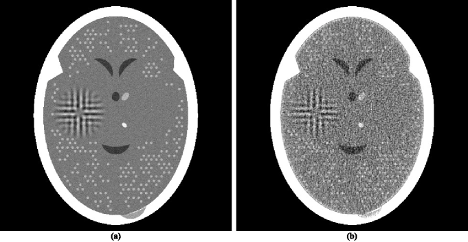
Figure 1: (a) A head phantom. (b) Reconstruction of the head phantom from realistically simulated projection data for 360 views using ART with blob basis functions.

For the selected head phantom we generated parallel projection data, in which one view comprises estimates of integrals through the phantom for a set of 693 equally-spaced parallel lines with a spacing of 0.0376 cm between them. (We chose to simulate parallel rather than divergent projection data, since the reconstruction by the method ofSIDK08a (42) with which we wish to compare the superiorization approach were performed for us by the authors ofSIDK08a (42) on parallel data. Even though contemporary CT scanners use divergent projection data, results obtained by the use of parallel projection data are relevant to them, since it is known that the quality of reconstructions from these two modes of data collection are very similar as long as the data generations use similar frequencies of sampling of lines and similar noise characteristics in the estimated integrals for those lines; see, for example, the reconstructions from divergent and parallel projection data in figure 5.15 of HERM09a (55).) In calculating these estimates we take into consideration the effects of photon statistics, detector width and scatter. Details of how we do this exactly can be found in Sections 5.5 and 5.9 of HERM09a (55). Briefly, quantum noise is calculated based on the assumption that approximately 2,000,000 photons enter the head along each ray, detector width is simulated by using 11 sub-rays along each of which the attenuation is calculated independently and then combined at the detector, and 5% of the photons get counted not by the detector for the ray in question but detectors for the neighboring rays. For the experiments in this paper, we did not simulate the poly-energetic nature of the x-ray source. To indicate what can be achieved in clinical CT, we show in figure 1(b) a reconstruction that was made from data comprising of 360 such views with the reconstruction algorithm known as ART with blob basis functions; see(HERM09a, 55, Chapter 11).

III.3 Superiorization reconstruction from a few views

The main reason in the literature for advocating the use of $TV$ as the optimization criterion is that by doing so one can achieve efficacious reconstructions even from sparsely sampled data. In our own workHERM08a (31) with realistically simulated CT data we found that this is not always the case and this will be demonstrated again by the experiments reported in the current paper.

There have appeared in the literature some approaches to $TV$ minimization that seem to indicate a more efficacious performance for CT than the one reported in HERM08a (31). One of these is the Adaptive Steepest Descent Projections Onto Convex Sets (ASD-POCS) algorithm, which is described in detail in the much-cited paper of Sidky and PanSIDK08a (42) and whose use has been since reported in a number of subsequent publications, for example, in SIDK11a (23, 43). We note that ASD-POCS was designed with the aim of producing an exact minimization algorithm, in contrast to our heuristic superiorization approach. Translating equations (6)-(8) of SIDK08a (42) into our terminology, the aim of ASD-POCS is the following: Given an $\varepsilon\in\mathbb{R}_{+}$, find an $\varepsilon$-compatible $\boldsymbol{x}\in\Omega=\mathbb{R}_{+}^{J}$ for which $TV(\boldsymbol{x})$ is minimal. (Note that this aim is a special case of the constrained optimization formulation presented in (10).) In order to test ASD-POCS, we generated realistic projection data as described in the previous subsection but for only 60 views at 3 degree increments with the spacing between the lines for which integrals are estimated set at 0.752 mm. Thus the number of rays (and hence the number photons put into the head) in this data set is a twelfth of what it is in the data set used to produce the reconstruction in figure 1(b). A reconstruction from these data was produced for us using ASD-POCS by the authors of SIDK08a (42) (this ensured that it does not suffer due to our misinterpretation of the algorithm or from our inappropriate choices of the free parameters), it is shown in figure 2(a).

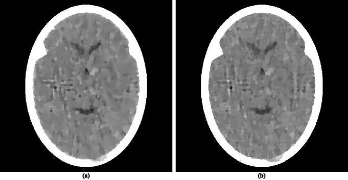
Figure 2: Reconstructions using $TV$ as the optimization criterion from realistically simulated projection data for 60 views using (a) ASD-POCS and (b) superiorization. As compared to figure 1(b), these reconstructions fail in two ways: they do not show some of the fine details in the phantom and they present some artifactual variations. The former of these is a consequence of reconstructing from a much smaller data set than used for figure 1(b). The latter is due to using a very narrow window (13.5 HU) in these displays. Were we to use a wider display window (e.g., from -429 HU to 429 HU) for the reconstructions in this figure and in figure 1(b), the visual appearance of the resulting images would be nearly indistinguishable.

Since the image quality of figure 2(a) is not anywhere near to that of figure 1(b), we present here a brief discussion as to why we are showing such images. Many publications in the recent medical imaging literature have claimed that medically-efficacious reconstructions can be obtained by the use of $TV$-minimization from data as sparse as what was used to produce figure 2(a). (In fact, ASD-POCS was motivated and used with such an aim in mindSIDK11a (23, 42, 43).) Such publications usually show reconstructions from sparse data as evidence for the validity of their claims. They can do this because in their presented illustrations the features that are observable in the reconstructions are usually much larger and/or of much higher contrast against their backgrounds than the small “tumors” in figure 1(a), which are perfectly visible in the reconstruction in figure 1(b), but are not detectable in the reconstruction from sparse data in figure 2(a). The reason why that reconstruction appears to be unacceptably bad is that the display window (from 0.204 cm^-1 linear attenuation coefficient to 0.21675 cm^-1 linear attenuation coefficient) is very narrow; it was selected to enhance the visibility of the small low-contrast tumors. The width of this window corresponds to about 13.5 Hounsfield Units (HU). As compared to this, in their evaluation of sparse-view reconstruction from flat-panel-detector cone-beam CT, Bian et al.BIAN10A (43) use what they call a “soft-tissue grayscale window” (also a “narrow window”) from -429 HU to 429 HU to display head phantom reconstructions. Using such a window for our reconstructions shown figures 2(a) and 1(b) would result in images that are nearly indistinguishable from each other. Thus reporting the images using such a display window is consistent with the claim that a TV-minimizing reconstruction from a few views is similar in quality to a more traditional reconstruction from many views. However, our much narrower display window reveals that this is not really so. We therefore continue using our much narrower window in what follows, since it clearly reveals the nature of the reconstructions being compared, warts and all.

While this ASD-POCS reconstruction is not as good as it should be for diagnostic CT of the brain (due to the sparsity of the data), it is visually better than the reconstruction using superiorization from similar data as reported inHERM08a (31). We discuss the reasons for this in the next subsection. Here we concentrate on examining whether one can achieve a reconstruction using superiorization that is as good as that produced by ASD-POCS from the same data.

For this we first need to examine the numerical properties of the ASD-POCS reconstruction. This reconstruction uses $485\times 485$ pixels each of size 0.376 mm by 0.376 mm. This implies that $J=235,225$ and it also determines the components of the vectors $\boldsymbol{a}^{i}\in\mathbb{R}^{J}$ in the precise specification of the problem $S$. The $Res_{S}$, as defined by (2), of the ASD-POCS reconstruction is 0.33 and the $TV$, as defined by (12), is 835.

We applied to the same problem $S$ a superiorized version of the algorithm $\mathbf{R}$ defined by (3). To complete the specification of $\mathbf{R}$, we point out that for the ordering of views we chose the “efficient” one that was introduced in HERM93a (58) and is also discussed on page 209 of HERM09a (55). The choices we made for the superiorization are the following: $\gamma_{\ell}=0.99995^{\ell}$, $\boldsymbol{\bar{x}}$ is the zero vector and $N=20$. The nonascending vector was computed by the method described in the paragraph below (12). Denoting by $R_{S}$ the infinite sequence of points in $\Omega$ that is produced by the superiorized version of the algorithm $\mathbf{R}$ when applied to the problem $S$, we chose as our reconstruction $\boldsymbol{x^{*}}=O\left(S,0.33,R_{S}\right)$. For such a reconstruction we have, by the definition of $O$, that $Res_{S}\left(\boldsymbol{x^{*}}\right)\leq 0.33$; in other words, the output of the superiorization algorithm is at least as constraints-compatible with $S$ as the output of ASD-POCS. From the point of view of $TV$-minimization, our $\boldsymbol{x^{*}}$ is slightly better: $TV\left(\boldsymbol{x^{*}}\right)=$826.

The superiorization reconstruction is displayed in figure 2(b). Visually it is similar to the reconstruction produced by ASD-POCS. From the optimization point of view it achieves the desired aim better than ASD-POCS does, since it results in smaller values for both $Res_{S}$ and for $TV$, even though only slightly.

That the two reconstructions in figure 2 are very similar is not surprising because a comparison of the pseudo-codes reveals that the ASD-POCS algorithm in SIDK08a (42) is essentially a special case of the Superiorized Version of Algorithm $\mathbf{P}$, even though it has been derived from rather different principles. To obtain the ASD-POCS algorithm from our methodology described here, we would have to choose an Algebraic Reconstruction Technique (ART; see Chapter 11 of HERM09a (55)) as the algorithm that we are superiorizing. Such a superiorization of ART was reported in the earliest paper on superiorization BUTN07a (27). For the illustration in our current paper we decided to superiorize the block-iterative algorithm $\mathbf{R}$ defined by (3). This illustrates the generality of the superiorization approach: it is applicable not only to a large class of constrained optimization problems, but also enables the use of any of a large class of iterative algorithms designed to produce a constraints-compatible solutions. A recent publication aimed at producing an exact $TV$-minimizing algorithm based on the block-iterative approach is DEFR11a (44).

III.4 Effects of variations in the reconstruction approach

The reconstruction in figure 2(a) produced by ASD-POCS definitely “looks better” than a reconstruction in HERM08a (31), which was obtained using superiorization from similar data. Since, as discussed in the last paragraph of the previous subsection, the ASD-POCS algorithm in SIDK08a (42) can be obtained as a special case of superiorization, it must be that some of the choices made in the details of the implementations are responsible for the visual differences. An analysis of the implementational details adopted by the two approaches revealed several differences. After removing these differences, the superiorization approach produced the image in figure 2(b), which is very similar to the reconstruction produced by ASD-POCS. We now list the implementational choices that were made for superiorization to make its performance match that of the reported implementation of ASD-POCS.

One implementational difference is in the stopping-rule of the iterative algorithm; that is, the choice of $\varepsilon$ in determining the output $O\left(S,\varepsilon,R_{S}\right)$. Since the data are noisy, the phantom itself does not match the data exactly. In previously reported implementations of superiorization it was assumed that the iterative process should terminate when an image is obtained that is approximately as constraints-compatible as the phantom; in the case of the phantom and the projections data on which we report here the value of $Res_{S}$ for the phantom is approximately 0.91, which is larger than its value (0.33) for the reconstruction produced by ASD-POCS. The output $O\left(S,0.91,R_{S}\right)$ is shown in figure 3(a). This is a wonderfully smooth reconstruction, its $TV$ value is only 771. However this smoothness comes at a price: we loose not only the ability to detect the large tumor, but we cannot even see anatomic features (such as the ventricular cavities) inside the brain. So it appears that, in order to see medically-relevant features in the brain, over-fitting (in the sense of producing a reconstruction from noisy data that is more constraints-compatible than the phantom) is desirable.

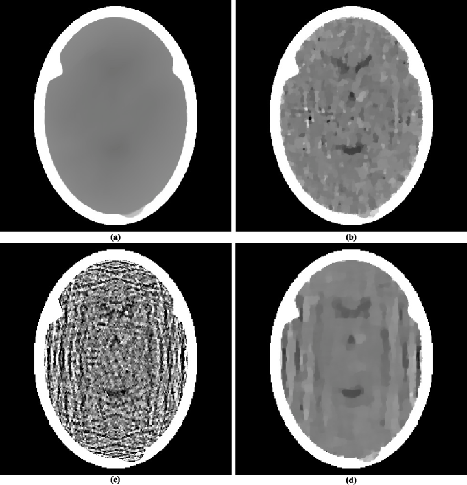
Figure 3: Reconstructions produced by varying some of the parameters in the algorithm that produced figure 2(b). (a) Changing the termination criterion form $\varepsilon=0.33$ to $\varepsilon=0.91.$ (b) Changing the value of $N$ from 20 to 1. (c) Reconstructing with pixel size 0.752 mm by 0.752 mm instead of 0.376 mm by 0.376 mm. (d) Reconstructing with all the three changes of (a)-(c).

In the implementations that produced previously reported reconstructions by superiorization, the number $N$ in the Superiorized Version of Algorithm $\mathbf{P}$ was always chosen to be 1. It is possible that this is the wrong choice, making only this change to what lead to the reconstruction in figure 2(b) results in the reconstruction shown in figure 3(b). That image appears similar to the image in figure 2(b), but it has a higher $TV$ value, namely 832, which is still very slightly lower than that of the ASD-POCS reconstruction. The choice $N=20$ was based on the desire to maintain consistency with what has been practiced using ASD-POCS, see page 4790 of SIDK08a (42). It appears that in the context of our paper the additional computing cost due to choosing $N$ to be 20 rather than 1 is not really justified. (We note that if $\boldsymbol{d}$ is selected using subgradients as discussed in the paragraph following (7) and thus $\boldsymbol{d}$ is not guaranteed to be a nonascending vector for the $TV$ function, then the choice of 20 rather than 1 for $N$ results in a considerable improvement. However, an even greater improvement is achieved even with $N=1$ by selecting $\boldsymbol{d}$ as recommended in this paper.)

Another important difference between the ASD-POCS implementation and the previous implementations of the superiorization approach is the size of the pixels in the reconstructions. For the ASD-POCS reconstruction this was selected to be 0.376 mm by 0.376 mm. In previously reported reconstructions by superiorization it was assumed that the edge of a pixel should be the same as the distance between the parallel lines along which the data are collected; that is, 0.752 mm for our problem $S$. This assumption proved to be false. $TV$-minimization takes care of undesirable artifacts that may otherwise arise due to the smaller pixels and this leads to a visual improvement. A superiorizing reconstruction with the larger pixels, using $\varepsilon=0.33$ and $N=20$, is shown in figure 3(c). (We note that the use of smaller pixels during iterative x-ray CT reconstructions was also suggested inZBIJ04a (59). However, that approach is quite different from what is presented here: its final result uses larger pixels whose values are obtained by averaging assemblies of values provided by the iterative process to the smaller pixels. There is no such downsampling in our approach, our final result is presented using the smaller pixels. Its smoothness is due to reduction of TV by the superiorization approach rather than to averaging pixel values in a denser digitization.)

Combining the use of the larger pixels with $\varepsilon=0.91$ and $N=1$ results in the reconstruction shown in figure 3(d). This reconstruction, for which the superiorization options were selected according to what was done inHERM08a (31), is visually inferior to those shown in our figure 2. The reconstructions displayed in figure 3 also illustrate another important point, namely that even though the mathematical results discussed in this paper are valid for a large range of choices of the parameters in the superiorization algorithms, for medical efficacy of the reconstructions attention has to be paid to these choices since they can have a drastic effect on the quality of the reconstruction.

It has been mentioned in Subsection II.2 that except for the presence of $\mathbf{Q}$ in (3), which enforces nonnegativity of the components, $\mathbf{R}$ is identical to the algorithm used and illustrated in HERM08a (31). It is known that CT reconstruction of the brain from many views does not suffer from ignoring the fact that the components of the $\boldsymbol{x}$, which represent linear attenuation coefficients, should be nonnegative; as is illustrated in figure 1(b). This remains so when reconstructing from a few views using the method and data that we have been discussing: if we do everything in exactly the same way as was done to obtain the reconstruction with $TV$ value 826 that is shown in our figure 2(b) but remove $\mathbf{Q}$ from (3), then we obtain a reconstruction in figure 4(a) whose $TV$ value is 829.

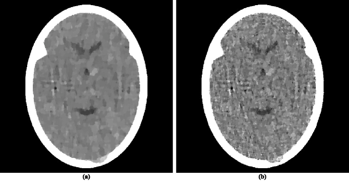
Figure 4: Reconstructions by variations that do not fit into the framework within which the previously shown reconstructions were produced. (a) Not using nonnegativity in the algorithm. (b) Interleaving perturbations with blocks.

Another variation that deserves discussion, because it has been suggested in the literature PENF10a (22), is one that does not come about by making choices for the general approach of the Superiorized Version of Algorithm $\mathbf{P}$ but rather by changing the nature of the approach. The variation in question is not applicable in general, but can be applied to the special case when the algorithm to be superiorized is the $\mathbf{R}$ defined by (3). It was suggested as an improvement to the approach presented above with the choice $N=1$. The idea was based on recognizing the block-iterative nature of the algorithmic operator $\mathbf{R}_{S}$ in (3) and intermingling the perturbation steps of lines (vii)-(xvii) of the Superiorized Version of Algorithm $\mathbf{R}$ with the projection steps $\mathbf{B}_{S_{1}},\ldots,\mathbf{B}_{S_{W}}$ of (3). It was reported in PENF10a (22) that doing this is advantageous to using the Superiorized Version of Algorithm $\mathbf{R}$. However, when we applied the variation of the Superiorized Version of Algorithm $\mathbf{R}$ that is proposed in PENF10a (22) to the problem $S$ that we have been using in this section, we ended up with the reconstruction in figure 4(b) whose $TV$ value is 920. This is not as good as what was obtained using the version of the algorithm that produced the reconstruction in figure 2(b). We conclude that the variation suggested by PENF10a (22), which does not fit into the theory of our paper, does not have an advantage over what we are proposing here, at least for the problem $S$ that we have been discussing in this section. We conjecture that the improvement reported in PENF10a (22) is due to selecting $\boldsymbol{d}$ using subgradients as discussed in the paragraph following (7) and, as discussed earlier, such an improvement is not obtained if $\boldsymbol{d}$ is selected by the more appropriate method recommended in this paper.

IV Discussion and Conclusions

Constrained optimization is an often-used tool in medical physics. The methodology of superiorization is a heuristic (as opposed to exact) approach to constrained optimization.

Although the idea of superiorization was introduced in 2007 and its practical use has been demonstrated in several publications since, this paper is the first to provide a solid mathematical foundation to superiorization as applied to the noisy problems of the real world. These foundations include a precise definition of constraints-compatibility, the concept of a strongly perturbation resilient algorithm, simple conditions that ensure that an algorithm is strongly perturbation resilient, the superiorized version of an algorithm and the showing that the superiorized version of a strongly perturbation resilient algorithm produces outputs that are essentially as constraints-compatible as those produced by the original version but are likely to have a smaller value of the chosen optimization criterion.

The approach is very general. For any iterative algorithm $\mathbf{P}$ and for any optimization criterion $\phi$ for which we know how to produce nonascending vectors, the pseudocode given in Subsection II.5 automatically provides the version of $\mathbf{P}$ that is superiorized for $\phi$.

We demonstrated superiorization for tomography when total variation is used as the optimization criterion. In particular, we illustrated on a particular tomography problem that, in spite of its generality, superiorization produced a reconstruction that is as good as (from the points of view of constraints-compatibility and $TV$-minimization) what was obtained by the ASD-POCS algorithm that was specially designed for $TV$-minimization in tomography.

Appendix

Conditions for strong perturbation resilience

Theorem 1.

Let $\mathbf{P}$ be an algorithm for a problem structure $\left\langle\mathbb{T},\mathcal{P}r\right\rangle$ such that, for all $T\in\mathbb{T}$, $\mathbf{P}$ is boundedly convergent for $T$, $\mathcal{P}r_{T}:\Omega\rightarrow\mathbb{R}$ is uniformly continuous and $\mathbf{P}_{T}:\Delta\rightarrow\Omega$ is nonexpansive. Then $\mathbf{P}$ is strongly perturbation resilient.

Proof.

We first show that there exists an $\varepsilon\in\mathbb{R}_{+}$ such that $O\left(T,\varepsilon,\left(\left(\mathbf{P}_{T}\right)^{k}\boldsymbol{x}\right)_{k=0}^{\infty}\right)$ is defined for every $\boldsymbol{x}\in\Omega$. Under the assumptions of the theorem, let $\gamma\in\mathbb{R}_{+}$ be such that $\mathcal{P}r_{T}\left(\boldsymbol{y}\left(\boldsymbol{x}\right)\right)\leq\gamma$, for every $\boldsymbol{x}\in\Omega$. We prove that $O\left(T,2\gamma,\left(\left(\mathbf{P}_{T}\right)^{k}\boldsymbol{x}\right)_{k=0}^{\infty}\right)$ is defined for every $\boldsymbol{x}\in\Omega$ as follows. Select a particular $\boldsymbol{x}\in\Omega$. By uniform continuity of $\mathcal{P}r_{T}$, there exists a $\delta>0$, such that $\left|\mathcal{P}r_{T}\left(\boldsymbol{z}\right)-\mathcal{P}r_{T}\left(\boldsymbol{y}\left(\boldsymbol{x}\right)\right)\right|\leq\gamma$, for any $\boldsymbol{z}\in\Omega$ for which $\left\|\boldsymbol{z}-\boldsymbol{y}\left(\boldsymbol{x}\right)\right\|\leq\delta$. Since $\mathbf{P}$ is convergent for $T$, there exists a nonnegative integer $K$, such that $\left\|\left(\mathbf{P}_{T}\right)^{K}\boldsymbol{x}-\boldsymbol{y}\left(\boldsymbol{x}\right)\right\|\leq\delta$. It follows that

$$\begin{array}[]{rcl}\left|\mathcal{P}r_{T}\left(\left(\mathbf{P}_{T}\right)^{K}\boldsymbol{x}\right)\right|&\leq&\left|\mathcal{P}r_{T}\left(\left(\mathbf{P}_{T}\right)^{K}\boldsymbol{x}\right)-\mathcal{P}r_{T}\left(\boldsymbol{y}\left(\boldsymbol{x}\right)\right)\right|+\left|\mathcal{P}r_{T}\left(\boldsymbol{y}\left(\boldsymbol{x}\right)\right)\right|\\ &\leq&2\gamma.\end{array}$$ (13)

Now let $T\in\mathbb{T}$ and $\varepsilon\in\mathbb{R}_{+}$ be such that $O\left(T,\varepsilon,\left(\left(\mathbf{P}_{T}\right)^{k}\boldsymbol{x}\right)_{k=0}^{\infty}\right)$ is defined for every $\boldsymbol{x}\in\Omega$. To prove the theorem, we need to show that $O\left(T,\varepsilon^{\prime},R\right)$ is defined for every $\varepsilon^{\prime}>\varepsilon$ and for every sequence $R=\left(\boldsymbol{x}^{k}\right)_{k=0}^{\infty}$ of points in $\Omega$ for which, for all $k\geq 0$, (6) is satisfied for bounded perturbations $\beta_{k}\boldsymbol{v}^{k}$ . Let $\varepsilon^{\prime}$ and $R$ satisfy the conditions of the previous sentence.

For $k\geq 0$, we have, due to the nonexpansiveness of $\mathbf{P}_{T}$, that

$$\left\|\boldsymbol{x}^{k+1}-\mathbf{P}_{T}\boldsymbol{x}^{k}\right\|=\left\|\mathbf{P}_{T}\left(\boldsymbol{x}^{k}+\beta_{k}\boldsymbol{v}^{k}\right)-\mathbf{P}_{T}\boldsymbol{x}^{k}\right\|\leq\left\|\beta_{k}\boldsymbol{v}^{k}\right\|.$$ (14)

Denote $\left\|\beta_{k}\boldsymbol{v}^{k}\right\|$ by $r_{k}$. Clearly, $r_{k}\in\mathbb{R}_{+}$ and it follows from the definition of bounded perturbations that ${\displaystyle\sum\limits_{k=0}^{\infty}}r_{k}\,<\infty$.

We next prove by induction that, for every pair of nonnegative integers $k$ and $i$,

$$\left\|\boldsymbol{x}^{k+i}-\left(\mathbf{P}_{T}\right)^{i}\boldsymbol{x}^{k}\right\|\leq{\displaystyle\sum_{j=k}^{k+i-1}r_{j}}.$$ (15)

Let $k$ be an arbitrary nonnegative integer. If $i=0$, then the value is zero on both sides of the inequality and hence (15) holds. Now assume that (15) holds for an integer $i\geq 0$. Then, by (14) and the nonexpansiveness of $\mathbf{P}_{T}$,

$$\begin{array}[]{rcl}\left\|\boldsymbol{x}^{k+i+1}-\left(\mathbf{P}_{T}\right)^{i+1}\boldsymbol{x}^{k}\right\|&\leq&\left\|\boldsymbol{x}^{k+i+1}-\mathbf{P}_{T}\boldsymbol{x}^{k+i}\right\|\\ &&+\left\|\mathbf{P}_{T}\boldsymbol{x}^{k+i}-\left(\mathbf{P}_{T}\right)^{i+1}\boldsymbol{x}^{k}\right\|\\ &\leq&r_{k+i}+\left\|\boldsymbol{x}^{k+i}-\left(\mathbf{P}_{T}\right)^{i}\boldsymbol{x}^{k}\right\|\\ &\leq&r_{k+i}+{\displaystyle\sum_{j=k}^{k+i-1}r_{j}}\\ &=&{\displaystyle\sum_{j=k}^{k+i}r_{j}},\end{array}$$ (16)

which completes our inductive proof. A consequence of (15) is that, for every pair of nonnegative integers $k$ and $i$,

$$\left\|\boldsymbol{x}^{k+i}-\left(\mathbf{P}_{T}\right)^{i}\boldsymbol{x}^{k}\right\|\leq{\displaystyle\sum_{j=k}^{\infty}r_{j}}.$$ (17)

Due to the summability of the nonnegative sequence $\left(r_{k}\right)_{k=0}^{\infty}$, the right-hand side (and hence the left-hand side) of this inequality gets arbitrarily close to zero as $k$ increases.

Since $\mathcal{P}r_{T}$ is uniformly continuous, there exists a $\delta$ such that, for all $\boldsymbol{x},\boldsymbol{y}\in\Omega$, $\left|\mathcal{P}r_{T}(\boldsymbol{x})-\mathcal{P}r_{T}(\boldsymbol{y})\right|\leq\varepsilon^{\prime}-\varepsilon$ provided that $\left\|\boldsymbol{x}-\boldsymbol{y}\right\|\leq\delta$. Select a $k$ so that $\sum_{j=k}^{\infty}r_{j}\leq\delta$. By the assumption that $O\left(T,\varepsilon,\left(\left(\mathbf{P}_{T}\right)^{k}\boldsymbol{x}\right)_{k=0}^{\infty}\right)$ is defined for every $\boldsymbol{x}\in\Omega$, there exists a nonnegative integer $i$ for which $\mathcal{P}r\left(\left(\mathbf{P}_{T}\right)^{i}\boldsymbol{x}^{k}\right)\leq\varepsilon$. From (17) we have, for this $k$ and $i$, that $\left\|\boldsymbol{x}^{k+i}-\left(\mathbf{P}_{T}\right)^{i}\boldsymbol{x}^{k}\right\|\leq\delta$ and, hence,

$$\begin{array}[]{rcl}\left|\mathcal{P}r_{T}(\boldsymbol{x}^{k+i})\right|&\leq&\left|\mathcal{P}r_{T}(\boldsymbol{x}^{k+i})-\mathcal{P}r_{T}\left(\left(\mathbf{P}_{T}\right)^{i}\boldsymbol{x}^{k}\right)\right|\\ &&+\left|\mathcal{P}r_{T}\left(\left(\mathbf{P}_{T}\right)^{i}\boldsymbol{x}^{k}\right)\right|\\ &\leq&\left(\varepsilon^{\prime}-\varepsilon\right)+\varepsilon=\varepsilon^{\prime},\end{array}$$ (18)

proving that $O\left(T,\varepsilon^{\prime},R\right)$ is defined. $\square$

Nonascending vectors for convex functions

Theorem 2.

Let $\phi:\mathbb{R}^{J}\rightarrow\mathbb{R}$ be a convex function and let $\boldsymbol{x}\in\mathbb{R}^{J}$. Let $\boldsymbol{g}\in\mathbb{R}^{J}$ satisfy the property: For 1$\leq j\leq J$, if the $j$th component $g_{j}$ of $\boldsymbol{g}$ is not zero, then the partial derivative $\frac{\partial\phi}{\partial x_{j}}(\boldsymbol{x})$ of $\phi$ at $\boldsymbol{x}$ exists and its value is $g_{j}$. Define $\boldsymbol{d}$ to be the zero vector if $\left\|\boldsymbol{g}\right\|=0$ and to be $-\boldsymbol{g}/\left\|\boldsymbol{g}\right\|$ otherwise. Then $\boldsymbol{d}$ is a nonascending vector for $\phi$ at $\boldsymbol{x}$.

Proof.

The theorem is trivially true if $\left\|\boldsymbol{g}\right\|=0$, so we assume that this is not the case. We denote by $I$ the nonempty set of those indices $j$ for which $g_{j}\neq 0$.

For $1\leq j\leq J$, let $s_{j}$ be $\nicefrac{{g_{j}}}{{\left|g_{j}\right|}}$ for $j\in I$ and be 0 otherwise, and let $\boldsymbol{e}^{j}\in\mathbb{R}^{J}$ be the vector all of whose components are zero except for the $j$th, which is one. Then, for $1\leq j\leq J$, there exists a $\delta_{j}>0$ such that, for $0\leq\lambda_{j}\leq\delta_{j}$,

$$\phi\left(\boldsymbol{x}-\lambda_{j}s_{j}\boldsymbol{e}^{j}\right)\leq\phi\left(\boldsymbol{x}\right).$$ (19)

This is obvious if $s_{j}=0$. Otherwise, $\frac{\partial\phi}{\partial x_{j}}(\boldsymbol{x})$ exists and indicates $\phi$ increases at $\boldsymbol{x}$ if $s_{j}=1$ or that $\phi$ decreases at $\boldsymbol{x}$ if $s_{j}=-1$. The existence of the desired $\delta_{j}$ can be derived from the standard definition of the partial derivative as a limit.

We define $\delta>0$ by

$$\delta=\frac{\left\|\boldsymbol{g}\right\|}{J}\min_{j\in I}\left\{\frac{\delta_{j}}{\left|g_{j}\right|}\right\}.$$ (20)

Then we have that, for $0\leq\lambda\leq\delta$,

$$\begin{array}[]{rcl}\phi\left(\boldsymbol{x}+\lambda\boldsymbol{d}\right)&=&\phi\left(\boldsymbol{x}-\lambda{\displaystyle\sum_{j=1}^{J}\frac{\left|g_{j}\right|}{\left\|\boldsymbol{g}\right\|}s_{j}}\boldsymbol{e}^{j}\right)\\ &=&\phi\left({\displaystyle\sum_{j=1}^{J}\frac{1}{J}\left(\boldsymbol{x}-\lambda J\frac{\left|g_{j}\right|}{\left\|\boldsymbol{g}\right\|}s_{j}\boldsymbol{e}^{j}\right)}\right)\\ &\leq&{\displaystyle\frac{1}{J}{\displaystyle\sum_{j=1}^{J}\phi\left(\boldsymbol{x}-\lambda J\frac{\left|g_{j}\right|}{\left\|\boldsymbol{g}\right\|}s_{j}\boldsymbol{e}^{j}\right)}}\\ &\leq&{\displaystyle\frac{1}{J}\sum_{j=1}^{J}}\phi\left(\boldsymbol{x}\right)\\ &=&\phi\left(\boldsymbol{x}\right).\end{array}$$ (21)

The first inequality above follows from the convexity of $\phi$ and the second one follows from (19), with $\lambda_{j}$ defined to be $\lambda J\frac{\left|g_{j}\right|}{\left\|\boldsymbol{g}\right\|}$, combined with (20). Thus $\boldsymbol{d}$ is a nonascending vector for $\phi$ at $\boldsymbol{x}$. $\square$

References

- (1) J. O. Deasy, “Multiple local minima in radiotherapy optimization problems with dose-volume constraints,” Med. Phys. 24, 1157–1161, (1997).
- (2) G. A. Ezzell, “Genetic and geometric optimization of three-dimensional radiation therapy treatment planning,” Med. Phys. 23, 293–305, (1996).
- (3) A. Gustafsson, B. K. Lind, and A. Brahme, “A generalized pencil beam algorithm for optimization of radiation-therapy,” Med. Phys. 21, 343–357, (1994).
- (4) A. Gustafsson, B. K. Lind, R. Svensson, and A. Brahme, “Simultaneous-optimization of dynamic multileaf collimation and scanning patterns or compensation filters using a generalized pencil beam algorithm,” Med. Phys. 22, 1141–1156, (1995).
- (5) E. Lessard and J. Pouliot, “Inverse planning anatomy-based dose optimization for hdr-brachytherapy of the prostate using fast simulated annealing algorithm and dedicated objective function,” Med. Phys. 28, 773–779, (2001).
- (6) R. Manzke, M. Grass, T. Nielsen, G. Shechter, and D. Hawkes, “Adaptive temporal resolution optimization in helical cardiac cone beam CT reconstruction,” Med. Phys. 30, 3072–3080, (2003).
- (7) A. B. Pugachev, A. L. Boyer, and L. Xing, “Beam orientation optimization in intensity-modulated radiation treatment planning,” Med. Phys. 27, 1238–1245, (2000).
- (8) D. M. Shepard, M. A. Earl, X. A. Li, S. Naqvi, and C. Yu, “Direct aperture optimization: A turnkey solution for step-and-shoot IMRT,” Med. Phys. 29, 1007–1018, (2002).
- (9) C. Studholme, D. L. G. Hill, and D. J. Hawkes, “Automated three-dimensional registration of magnetic resonance and positron emission tomography brain images by multiresolution optimization of voxel similarity measures,” Med. Phys. 24, 25–35, (1997).
- (10) Q. W. Wu and R. Mohan, “Algorithms and functionality of an intensity modulated radiotherapy optimization system,” Med. Phys. 27, 701–711, (2000).
- (11) Y. Yu and M. C. Schell, “A genetic algorithm for the optimization of prostate implants,” Med. Phys. 23, 2085–2091, (1996).
- (12) T. Z. Zhang, R. Jeraj, H. Keller, W. G. Lu, G. H. Olivera, T. R. McNutt, T. R. Mackie, and B. Paliwal, “Treatment plan optimization incorporating respiratory motion,” Med. Phys. 31, 1576–1586, (2004).
- (13) M. Abdoli, M. R. Ay, A. Ahmadian, R. A. Dierckx, and H. Zaidi, “Reduction of dental filling metallic artifacts in CT-based attenuation correction of PET data using weighted virtual sinograms optimized by a genetic algorithm,” Med. Phys. 37, 6166–6177, (2010).
- (14) S. Bartolac, S. Graham, J. Siewerdsen, and D. Jaffray, “Fluence field optimization for noise and dose objectives in CT,” Med. Phys. 38, S2–S17, (2011).
- (15) W. Chen, D. Craft, T. M. Madden, K. Zhang, H. M. Kooy, and G. T. Herman, “A fast optimization algorithm for multicriteria intensity modulated proton therapy planning,” Med. Phys. 37, 4938–4945, (2010).
- (16) J. Fiege, B. McCurdy, P. Potrebko, H. Champion, and A. Cull, “PARETO: A novel evolutionary optimization approach to multiobjective IMRT planning,” Med. Phys. 38, 5217–5229, (2011).
- (17) A. Fredriksson, A. Forsgren, and B. Hardemark, “Minimax optimization for handling range and setup uncertainties in proton therapy,” Med. Phys. 38, 1672–1684, (2011).
- (18) C. Holdsworth, M. Kim, J. Liao, and M. H. Phillips, “A hierarchical evolutionary algorithm for multiobjective optimization in IMRT,” Med. Phys. 37, 4986–4997, (2010).
- (19) C. Holdsworth, R. D. Stewart, M. Kim, J. Liao, and M. H. Phillips, “Investigation of effective decision criteria for multiobjective optimization in IMRT,” Med. Phys. 38, 2964–2974, (2011).
- (20) T. Kim, L. Zhu, T.-S. Suh, S. Geneser, B. Meng, and L. Xing, “Inverse planning for IMRT with nonuniform beam profiles using total-variation regularization (TVR),” Med. Phys. 38, 57–66, (2011).
- (21) C. Men, H. E. Romeijn, X. Jia, and S. B. Jiang, “Ultrafast treatment plan optimization for volumetric modulated arc therapy (VMAT),” Med. Phys. 37, 5787–5791, (2010).
- (22) S. N. Penfold, R. W. Schulte, Y. Censor, and A. B. Rosenfeld, “Total variation superiorization schemes in proton computed tomography image reconstruction,” Med. Phys. 37, 5887–5895, (2010).
- (23) E. Y. Sidky, Y. Duchin, X. Pan, and C. Ullberg, “A constrained, total-variation minimization algorithm for low-intensity x-ray CT,” Med. Phys. 38, S117–S125, (2011).
- (24) H. Stabenau, L. Rivera, E. Yorke, J. Yang, R. Lu, R. J. Radke, and A. Jackson, “Reduced order constrained optimization (ROCO): Clinical application to lung IMRT,” Med. Phys. 38, 2731–2741, (2011).
- (25) Y. Yang and M. J. Rivard, “Dosimetric optimization of a conical breast brachytherapy applicator for improved skin dose sparing,” Med. Phys. 37, 5665–5671, (2010).
- (26) X. Zhang, J. Wang, and L. Xing, “Metal artifact reduction in x-ray computed tomography (CT) by constrained optimization,” Med. Phys. 38, 701–711, (2011).
- (27) D. Butnariu, R. Davidi, G. T. Herman, and I. G. Kazantsev, “Stable convergence behavior under summable perturbations of a class of projection methods for convex feasibility and optimization problems,” IEEE J. Sel. Top. Sign. Process. 1, 540–547, (2007).
- (28) R. Davidi, G. T. Herman, and Y. Censor, “Perturbation-resilient block-iterative projection methods with application to image reconstruction from projections,” Int. Trans. Oper. Res. 16, 505–524, (2009).
- (29) Y. Censor, R. Davidi, and G. T. Herman, “Perturbation resilience and superiorization of iterative algorithms,” Inverse Probl. 26, 065008, (2010).
- (30) T. Nikazad, R. Davidi, and G. T. Herman, “Accelerated perturbation-resilient block-iterative projection methods with application to image reconstruction,” Inverse Probl. 28, 035005, (2012).
- (31) G. T. Herman and R. Davidi, “Image reconstruction from a small number of projections,” Inverse Probl. 24, 045011, (2008).
- (32) E. Garduño, R. Davidi, and G. T. Herman, “Reconstruction from a few projections by -minimization of the Haar transform,” Inverse Probl. 27, 055006, (2011).
- (33) R. L. Rardin and R. Uzsoy, “Experimental evaluation of heuristic optimization algorithms: A tutorial,” J. Heuristics 7, 261–304, (2001).
- (34) L. Wernisch, S. Hery, and S. J. Wodak, “Automatic protein design with all atom force-fields by exact and heuristic optimization,” J. Mol. Biol. 301, 713–736, (2000).
- (35) S. H. Zanakis and J. R. Evans, “Heuristic optimization - why, when, and how to use it,” Interfaces 11, 84–91, (1981).
- (36) G. T. Herman and W. Chen, “A fast algorithm for solving a linear feasibility problem with application to intensity-modulated radiation therapy,” Linear Algebra Appl. 428, 1207–1217, (2008).
- (37) E. S. Helou Neto and Á. R. De Pierro, “Incremental subgradients for constrained convex optimization: A unified framework and new methods,” SIAM J. Optimiz. 20, 1547–1572, (2009).
- (38) E. S. Helou Neto and Á. R. De Pierro, “On perturbed steepest descent methods with inexact line search for bilevel convex optimization,” Optimization 60, 991–1008, (2011).
- (39) E. A. Nurminski, Envelope stepsize control for iterative algorithms based on Fejer processes with attractants, Optimiz. Method. Softw. 25, 97–108, (2010).
- (40) P. L. Combettes and J. Luo, “An adaptive level set method for nondifferentiable constrained image recovery,” IEEE Trans. Image Proc. 11, 1295–1304, (2002).
- (41) P. L. Combettes and J.-C. Pesquet, “Image restoration subject to a total variation constraint,” IEEE Trans. Image Proc. 13, 1213–1222, (2004).
- (42) E. Y. Sidky and X. Pan, “Image reconstruction in circular cone-beam computed tomography by constrained, total-variation minimization,” Phys. Med. Biol. 53, 4777–4807, (2008).
- (43) J. Bian, J. H. Siewerdsen, X. Han, E. Y. Sidky, J. L Prince, C. A. Pelizzari and X. Pan, “Evaluation of sparse-view reconstruction from flat-panel-detector cone-beam CT,” Phys. Med. Biol. 55, 6575–6599, (2010).
- (44) M. Defrise, C. Vanhove, and X. Liu, “An algorithm for total variation regularization in high-dimensional linear problems,” Inverse Probl. 27, 065002, (2011).
- (45) Y. Censor, W. Chen, P. L. Combettes, R. Davidi, and G. T. Herman, “On the effectiveness of projection methods for convex feasibility problems with linear inequality constraints,” Comput. Optim. Appl. 51, 1065–1088, (2012).
- (46) J. Bioucas-Dias and M. Figueiredo, “A new TwIST: two-step iterative shrinkage/thresholding algorithms for image restoration,” IEEE Trans. Image Proc. 16, 2992–3004, (2007).
- (47) T. Goldstein and S. Osher, “The split Bregman method for L1 regularized problems,” SIAM J. Imaging Sci. 2, 323–343, (2009).
- (48) L. A. Shepp and Y. Vardi, “Maximum likelihood reconstruction for emission tomography,” IEEE Trans. Med. Imag. 1, 113–122. (1982).
- (49) E. Levitan and G. T. Herman, “A maximum a posteriori probability expectation maximization algorithm for image reconstruction in emission tomography,” IEEE Trans. Med. Imag. 6:185–192, (1987).
- (50) W. Jin, Y. Censor and M. Jiang, “A heuristic superiorization-like approach to bioluminescence tomography,” in Proceedings of the International Federation for Medical and Biological Engineering (IFMBE) (Springer-Verlag, 2012), to appear.
- (51) H. M. Hudson and R. S. Larkin, “Accelerated image reconstruction using ordered subsets of projection data,” IEEE Trans. Med. Imag. 13, 601–609, (1994).
- (52) T. Elfving, “Block-iterative methods for consistent and inconsistent linear equations,” Numer. Math. 35, 1–12, (1980).
- (53) P. P. B. Eggermont, G. T. Herman, and A. Lent, “Iterative algorithms for large partitioned linear systems, with applications to image reconstruction,” Linear Algebra Appl. 40, 37–67, (1981).
- (54) R. Aharoni and Y. Censor, “Block-iterative projection methods for parallel computation of solutions to convex feasibility problems,” Linear Algebra Appl. 120, 165–175, (1989).
- (55) G. T. Herman, Fundamentals of Computerized Tomography: Image Reconstruction from Projections, 2nd ed., Springer, 2009.
- (56) J. F. P. J. Abascal, J. Chamorro-Servent, J. Aguirre, S. Arridge, T. Correia, J. Ripoli, J. J. Vaquero, and M. Desco, “Fluorescence diffuse optical tomography using the split Bregman method,” Med. Phys. 38, 6275–6284, (2011)
- (57) R. Davidi, G. T. Herman, and J. Klukowska, SNARK09: A Programming System for the Reconstruction of 2D Images from 1D Projections, http://www.snark09.com, 2009.
- (58) G. T. Herman and L. B. Meyer, “Algebraic reconstruction techniques can be made computationally efficient,” IEEE Trans. Med. Imag. 12, 600–609, (1993).
- (59) W. Zbijewski and F. J. Beekman, “Characterization and suppression of edge and aliasing artefacts in iterative x-ray CT reconstruction,” Phys. Med. Biol. 49, 145–157, (2004).