Short-time dynamics and high-frequency rheology of core-shell suspensions with thin-shells

Abstract

Short-time dynamics and high-frequency rheology for suspensions of non-overlapping core-shell particles with thin shells were analysed. In the thin-shell limit, the single-particle scattering coefficients were derived and shown to define a unique effective radius. This result was used to justify theoretically (in the thin-shell limit) the accuracy of the annulus approximation with the inner radius equal to the effective hydrodynamic radius of the core-shell particle. The two-particle virial expansion of the translational & rotational self-diffusion, sedimentation and viscosity was performed. The virial coefficients were evaluated and shown to be accurately approximated by the effective annulus model, in contrast to the imprecise effective hard sphere model.

I Introduction

Recently, there has been a growing interest in micro and nanogels, and other permeable particles, which can be used to carry drugs or proteins Kasper:98 -Fuchs:12 . For such systems, density of polymer segments inside the core region is frequently much higher than in the outer part, and therefore they are often approximated as core-shell particles.

A core-shell particle consists of a solid core of radius $a$, and a surrounding permeable shell, with the inner and outer radii, $a$ and $b$, respectively (see Fig. 1). The porous medium inside the shell is characterized by the uniform hydrodynamic penetration depth $\kappa^{-1}$. It is assumed that the particles do not overlap, i.e. their centers cannot come closer to each other than $2b$.

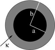
Figure 1: The core-shell particle: the solid core of radius $a$ is surrounded by the uniformly permeable shell of radii $a$, $b$ and the hydrodynamic penetration depth $\kappa^{-1}$.

In a recent paper Abade:12 , the precise multipole method was applied to extensively analyze dynamics and rheology of core shell particles. High-frequency viscosity, short-time translational and rotational diffusion, and sedimentation coefficient have been evaluated numerically for a very wide range of permeabilities of both wide and thin shells, with volume fractions up to $\phi=0.45$. It was concluded that for wide shells with a low permeability ($\kappa(b-a)\gtrsim 5$), the core is practically invisible and particles behave as uniformly permeable.

In the oposite limit of thin shells, it was shown that the core-shell particles cannot be well-approximated by hard spheres of radius $b$, even for a tiny, hardly permeable shell. However, the dynamics of concentrated core-shell systems is well reproduced, if a thin permeable shell is replaced by the shell of the pure fluid (the so-called annulus model Felderhof_Cichocki:91 ). The difference between the hard spheres and annulus particles of the same radii $b$ is very large; for example, 20-35% for the diffusion and sedimentation, and 60% for the viscosity, if $(b-a)/a=0.05$, $\kappa a=10$, and $\phi=0.45$. The shell influence cannot be neglected, and the essential reason is that it prevents particles from overlapping.

This result indicates that a more detailed analysis of the thin-shell limit is needed. For dilute systems of non-interacting core-shell particles, the single-particle translational & rotational diffusion coefficients and intrinsic viscosity determine the corresponding hydrodynamic radii $a_{\text{eff}}$ Masliyah:87 ; ChenYe:00 ; Zackrisson_Bergenholtz:03 ; Cichocki_Felderhof:09 , which, in general, are only tenuously connected to the geometrical radius $a$ of the core-shell particle Zackrisson_Bergenholtz:03 . A thin-shell analysis of such systems has been recently performed in Ref. Zackrisson_Bergenholtz:03 . The leading terms of $a_{\text{eff}}$ have been given and shown to be the same for the intrinsic viscosity and the translational diffusion.

In this paper, we extend the idea of Ref. Zackrisson_Bergenholtz:03 , and we investigate the thin-shell limit for concentrated systems of the core-shell particles. We use the general concept of the hydrodynamic radius model (HRM) Abade_JCP:2010 , where the effective radius approximation is restricted only to the hydrodynamic interaction, with no modification of direct interactions. In this work, the direct interactions between core-shell particles are specified by the no-overlap radius $b$. In this case, the HRM model is equivalent to the effective annulus model with the no-overlap radius of the outer shell $b$ and the radius of the inner shell equal to the hydrodynamic radius $a_{\text{eff}}$ of the core-shell particle. We will show that the effective annulus approximation is much more precise than the standard model of a hard-core particle with the effective radius $a_{\text{eff}}$.

The paper is organized as follows. Sec. II contains theoretical description of the core-shell suspensions. Sec. III is focused on the hydrodynamics of the single core-shell particles with thin shells. In Sec. IV, direct (no-overlap) interactions between core-shell particles are described within the annulus model. In Sec. V, the thin-shell limit of the two-particle virial coefficients is explicitly carried out for the translational & rotational self-diffusion, sedimentation and effective viscosity, and accuracy of the effective annulus model is examined. The conclusions are presented in Sec. VI.

II The core-shell suspensions

We consider a fluid of shear viscosity $\eta_{0}$, with randomly distributed identical core-shell particles Cichocki_Felderhof:09 defined in Sec. I and shown in Fig. 1.

Geometry of the particle is characterized by the relative thickness of the porous shell,

$$\epsilon=\frac{b-a}{a}.$$ (1)

The effect of the particle permeability is described by the ratio $x$ of the particle radius $a$ to the hydrodynamic screening length $\kappa^{-1}$ of the uniformly porous material inside the particle, i.e.

$$x = \kappa a.$$ (2)

All the distances are normalized by the core radius $a$.

The fluid flow is characterized by the low-Reynolds-number, Re$<<$1. Outside the particles, the fluid velocity ${\bm{v}}$ and pressure $p$ satisfy the Stokes equations Kim-Karrila:1991 ; Happel-Brenner:1986 ,

$$\eta_{0}\;\!{\bm{\nabla}}^{2}{\bm{v}}({\bm{r}})-{\bm{\nabla}}p({\bm{r}}) = 0$$

$${\bm{\nabla}}\cdot{\bm{v}}({\bm{r}}) = 0,$$ (3)

and inside the particle shells, by the Brinkman-Debye-Büche (BDB) equations Brinkman:47 ; DebyeBueche:48 ,

$$\eta_{0}\;\!{\bm{\nabla}}^{2}{\bm{v}}({\bm{r}})-\eta_{0}\;\!\kappa^{2}\left[{\bm{v}({\bm{r}})}-{\bm{u}}_{i}({\bm{r}})\right]-{\bm{\nabla}}p({\bm{r}}) = 0$$

$${\bm{\nabla}}\cdot{\bm{v}}({\bm{r}}) = 0.$$ (4)

The core and the skeleton of the particle $i$, centered at ${\bf r}_{i}$, move rigidly with the local velocity ${\bf u}_{i}({\bf r})={\bf U}_{i}+{\bm{\Omega}}_{i}\times\left({\bf r}-{\bf r}_{i}\right)$, determined by their translational and rotational velocities ${\bf U}_{i}$ and ${\bm{\Omega}}_{i}$, respectively. The fluid velocity and the stress are continuous across the particle surface, i.e. at $|{\bf r}-{\bf r}_{i}|=b$. The fluid sticks to the core surface; that is, ${\bm{v}}=0$ at $|{\bf r}-{\bf r}_{i}|=a$.

The coupled Stokes-BDB problem defined above is solved by the multipole expansion CFHWB:94 ; E-JW:2009 . Many-particle mobility coefficients are evaluated and averaged over the statistical equilibrium ensemble of configurations, resulting in the short-time self-diffusion, sedimentation and high-frequency viscosity coefficients, see e.g. Refs. m1 ; m2 ; m3 ; m4 ; Abade:12 for the general theoretical scheme. The important issue discussed in this work is that the N-particle mobility coefficients $\mbox{\boldmath$\mu$}_{ij}(1...N)$ are determined in terms of the Green operators ${\bf G}(mn)$ (which depend on the distance between particles $m$ and $n$), and the single-particle friction operators, ${\bf Z}_{0}(k)$ and $\hat{\bf Z}_{0}(k)$ (which depend on the internal structure and size of a particle $k$ Cichocki_Felderhof_Schmitz:88 ). This relation can be written as a scattering series,

$$\mbox{\boldmath$\mu$}_{ij}(1...N)\!\!\!=\!\!\!\delta_{ij}\,\mbox{\boldmath$\mu$}_{0}(i)+\mbox{\boldmath$\mu$}_{0}(i)\,{\bf Z}_{0}(i)\sum^{N}_{k=1}\left[\delta_{ik}\right.$$

$$\left.-(\!1\!\!-\!\delta_{ik}\!)\,{\bf G}(ik)\,\hat{\bf Z}_{0}(k)\!+...\right](\!1\!\!-\!\delta_{kj}\!)\,{\bf G}(kj)\,{\bf Z}_{0}(j)\,\mbox{\boldmath$\mu$}_{0}(j).$$

(5)

or in short as

$$\mbox{\boldmath$\mu$}=\mbox{\boldmath$\mu$}_{0}+\mbox{\boldmath$\mu$}_{0}\;{\mathbf{Z}}_{0}\;\frac{1}{{\bf 1}+{\bf G}\hat{{\mathbf{Z}}}_{0}}\;{\bf G}\;{\mathbf{Z}}_{0}\;\mbox{\boldmath$\mu$}_{0},$$ (6)

with $\mbox{\boldmath$\mu$}_{0}$ denoting the single-particle mobility operator (determined by the inverse of ${\bf Z}_{0}$). The single-particle friction operators, ${\bf Z}_{0}$ and $\hat{\bf Z}_{0}$, determine the hydrodynamic force density exerted by a given ambient flow on a motionless and a freely moving particle, respectively. The matrix elements of these operators are the single particle scattering coefficients $A_{l\sigma}$, with $l\!=\!1,2,3,4,...$ and $\sigma\!=\!1,2,3$  Cichocki_Felderhof_Schmitz:88 , see Appendix A for the explicit relation. If the ambient fluid flow is decomposed into the multipole components Lamb , labeled by $\sigma,\,l$ and $m\!=\!0,...,\pm l$, then $A_{l\sigma}$ determine the corresponding multipoles of the fluid velocity, reflected (scattered) by a particle immersed in a given ambient flow. This is why $A_{l\sigma}$ are called “scattering coefficients”Cichocki_Felderhof:09 ; Cichocki_Felderhof_Schmitz:88 . In the multipole approach, differences in the internal structure of particles (e.g. solid, liquid, gas, porous, core-shell, stick-slip), are fully accounted by different scattering coefficients. The other parts of the multipole algorithm need not to be changed. In particular, the scattering coefficeints $A_{10},\;A_{11}$ and $A_{20}$ determine the single-particle translational, $D_{0}^{t}$, and rotational, $D_{0}^{r}$, diffusion coefficients and the intrinsic viscosity, $\bar{\left[\eta\right]}$, by the following relations,

$$\bar{\left[\eta\right]} = \frac{3\mu_{0}^{d}}{8\pi\eta_{0}a^{3}},$$ (7)

$$D_{0}^{t} = k_{B}T\mu_{0}^{t},$$ (8)

$$D_{0}^{r} = k_{B}T\mu_{0}^{r},$$ (9)

with the corresponding single-particle mobility coefficients,

$$\mu_{0}^{d} = \frac{8\pi\eta_{0}A_{20}}{3},$$ (10)

$$\mu_{0}^{t} = \frac{1}{4\pi\eta_{0}A_{10}},$$ (11)

$$\mu_{0}^{r} = \frac{1}{8\pi\eta_{0}A_{11}}.$$ (12)

For core-shell particles, the dependence of all the scattering coefficeints $A_{l\sigma}$ on $(x,a,b)$ have been determined analytically in Ref. Cichocki_Felderhof:09 .

III Single core-shell particles with thin shells

In this section, we perform asymptotic expansion of the core-shell model in the thin-shell limit, i.e. when

$$a,\kappa=\mbox{const}\;\;\mbox{ and }\;\;\epsilon\rightarrow 0.$$ (13)

The asymptotic expansion of all the single-particle scattering coefficients $A_{l\sigma}(x,a,b)$, derived in Ref. Cichocki_Felderhof:09 , in the thin-shell limit (13), is the following,

$$A_{l\sigma}(x,a,b) = A_{l\sigma}^{hs}(a)[1+\alpha_{l\sigma}x^{2}\epsilon^{3}/3+...],$$ (14)

$$B_{l2}(x,a,b) = B_{l2}^{hs}(a)[1+\beta_{l2}x^{2}\epsilon^{3}/3+...],$$ (15)

where $l=1,2,...$, $\sigma=0,1,2$,

$$\alpha_{l0} = {2l-1},$$ (16)

$$\alpha_{l1} = \alpha_{l2}={2l+1},$$ (17)

$$\beta_{l2} = {2l+3},$$ (18)

and the terms omitted in Eqs. (14)-(15) scale as $\sim x^{2}\epsilon^{4}$.

Above, $A_{l\sigma}^{hs}(a)$ and $B_{l2}^{hs}(a)$ denote the scattering coefficients for a hard sphere of radius $a$ Cichocki_Felderhof_Schmitz:88 , listed in Appendix A. Taking into account that

$$A_{l0}^{hs}(a) \sim a^{2l-1}=a^{\alpha_{l0}},$$ (19)

$$A_{l1}^{hs}(a),A_{l2}^{hs}(a) \sim a^{2l+1}=a^{\alpha_{l1}}=a^{\alpha_{l2}},$$ (20)

$$B_{l2}^{hs}(a) \sim a^{2l+3}=a^{\alpha_{l2}},$$ (21)

and using the relation,

$$a^{k}(1+k\psi)\stackrel{{\scriptstyle\psi\rightarrow 0}}{{\approx}}[a(1+\psi)]^{k},$$ (22)

with $\psi=x^{2}\epsilon^{3}/3$ and $k=\alpha_{l\sigma},\beta_{l\sigma}$, we can combine the leading terms of the asymptotic expansion (14)-(15), and write it in the following compact form,

$$A_{l\sigma}(x,a,b) = A_{l\sigma}^{hs}(a_{\text{eff}})[1+{\cal O}(\epsilon^{4})],$$ (23)

$$B_{l2}(x,a,b) = B_{l2}^{hs}(a_{\text{eff}})[1+{\cal O}(\epsilon^{4})],$$ (24)

with the universal $a_{\text{eff}}$ for all the multipole indices,

$$a_{\text{eff}}/a=1+\frac{1}{3}x^{2}\epsilon^{3}+{\cal O}(\epsilon^{4}),$$ (25)

and the ${\cal O}(\epsilon^{4})$ terms $\sim x^{2}\epsilon^{4}$. The above relations show that in the leading order of the thin-shell expansion, the core-shell scattering coefficients are equal to the scattering coefficients $A_{l\sigma}^{hs}(a_{\text{eff}})$ and $B_{l2}^{hs}(a_{\text{eff}})$ of a hard sphere with the effective radius $a_{\text{eff}}$. This result is the important generalization of the thin-shell analysis performed in Ref. Zackrisson_Bergenholtz:03 for the intrinsic viscosity and translational self-diffusion.

In Ref. Zackrisson_Bergenholtz:03 it was shown that the hydrodynamic radii, defined by the intrinsic viscosity,

$$a_{\text{eff},\eta} = \left(\frac{2}{5}A_{20}\right)^{\!\!1/3},$$ (26)

and the translational diffusion coefficient of single core-shell particles Masliyah:87 ,

$$a_{\text{eff},t}=\frac{2}{3}A_{10},$$ (27)

have the same leading terms (25) in the thin-shell expansion.

We find out that all the scattering coefficients $A_{l\sigma}(x,a,b)$, up to terms $\sim(x^{2}\epsilon^{3})$, are determined by the same effective radius (25). In particular, also the hydrodynamic radius defined by the single-particle rotational diffusion coefficient ChenYe:00 ,

$$a_{\text{eff},r} = A_{11}^{1/3}.$$ (28)

As discussed in the previous section, the many-body hydrodynamic interactions depend on the particle internal structure only through the scattering coeffcients. The result is that in the thin-shell expansion (13) the hydrodynamic interactions between core-shell particles consist of the dominant contribution from the hard spheres with the effective radius, plus a small correction which depends on a single parameter $x^{2}\epsilon^{4}$.

In the next section, the single-particle scattering coefficients will be used to construct a model for the concentrated suspensions of core-shell particles.

IV Annulus model

For semi-dilute and concentrated suspensions, direct interactions between particles have to be taken into account. In the annulus model Felderhof_Cichocki:91 , these interactions are taken into account by introducing a non-overlap radius $b$, which surrounds a hard sphere of radius $c$, which is smaller than $b$. The shell of the relative thickness $\delta$,

$$\delta=\frac{b-c}{c},$$ (29)

is filled with the same fluid as outside the annulus particle, see Fig. 2. The annulus model can in general be applied for particles of a different internal structure and a different type of direct interactions.

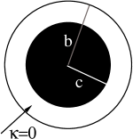
Figure 2: The annulus particle: the solid core of radius $c$ is surrounded by a completely permeable ($\kappa\!=\!0$) shell with the no-overlap radius $b$.

Transport coefficients of semi-dilute and concentrated core-shell suspensions, such as the translational & rotational self-diffusion, sedimentation and viscosity coefficients, are evaluated as statistical averages of the corresponding many-particle mobilities. The leading contributions to the moblilities of the core-shell particles with the outer and inner radii $b$ and $a$ (see Fig. 1) come from the hydrodynamic intractions of the hard-spheres with effective radii $a_{\text{eff}}$, larger than $a$ and smaller than $b$. On the other hand, the averaging takes into account the no-overlap condition - the particle centers have to be separated by a distance at least twice as large as the outer shell radius $b$. Therefore, the dynamics of many core-shell particles is approximated within the (effective) annulus model with $c=a_{\text{eff}}$ and the non-overlap radius $b$ the same as for the core-shell particle, see Fig. 3.

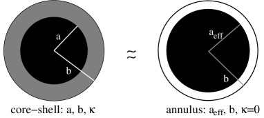
Figure 3: In the dynamics of concentrated suspensions, a core-shell particle with a thin shell is well-approximated by the annulus model with the hydrodynamic inner radius $c=a_{\text{eff}}$.

The corresponding effective hydrodynamic shell thickness,

$$\epsilon_{\text{eff}}=\frac{b-a_{\text{eff}}}{a_{\text{eff}}}.$$ (30)

V Example of the thin-shell analysis: viral expansion of the transport coefficients

In this Section, we will explicitly perform the thin-shell expansion for the two-particle virial contribution to the translational and rotatinal self-diffusion, sedimentation and high-frequency viscosity, and compare the results with the effective annulus approximation.

V.1 Virial expansion

The virial expansion of the transport coefficients for suspensions of core-shell particles is carried out using the inner radius $a$ as the reference one, i.e. we expand in powers of the volume fraction,

$$\phi_{a}=\frac{4}{3}\pi na^{3}.$$ (31)

The short-time translational and rotational self-diffusion coefficients, $D_{t}$ and $D_{r}$, the sedimentation coefficient $K$, and the high-frequency viscosity $\eta_{\infty}$ have the following virial expansion,

$$D_{t}/D_{0}^{t} = 1+\bar{\lambda}_{t}\phi_{a}+{\cal O}(\phi_{a}^{2}),$$ (32)

$$D_{r}/D_{0}^{r} = 1+\bar{\lambda}_{r}\phi_{a}+{\cal O}(\phi_{a}^{2}),$$ (33)

$$K = 1+\bar{\lambda}_{K}\phi_{a}+{\cal O}(\phi_{a}^{2}),$$ (34)

$$\eta_{\infty}/\eta_{0} = 1+\bar{[\eta]}\phi_{a}+\bar{\lambda}_{\eta}\phi_{a}^{2}+{\cal O}(\phi_{a}^{3}),$$ (35)

with the single core-shell particle translational & rotational diffusion coefficients, and the intrinsic viscosity defined in Eqs. (8)-(12). The bar over the virial coefficients reminds that they correspond to the expansion with respect to volume fraction based on the inner radius (rather than the outer one).

The explicit theoretical expressions for the two-particle virial coefficients $\bar{\lambda}\!\equiv\!\bar{\lambda}_{t},\bar{\lambda}_{K},\bar{\lambda}_{r}$ and $\bar{\lambda}_{\eta}$ are derived in Appendix B. In Sec. V.3, they are used to evaluate $\bar{\lambda}(x,\epsilon)$ numerically in a wide range of the parameters.

V.2 Annulus model

An annulus particle, introduced in Sec. IV and illustrated in Fig 2, is described by two parameters: the hard core radius $c$ and the no-overlap radius $b$. The corresponding shell thickness $\delta$ is defined in Eq. (29). With the use of the volume fraction $\phi_{c}=4\pi nc^{3}/3$, the annulus two-particle virial coefficients $\bar{\lambda}^{A}(\delta)$ of the translational and rotational self-diffusion, sedimentation and viscosity are defined by the analogs of Eqs. (32)-(35) with $\phi_{a}\rightarrow\phi_{c}$, and the single core-shell particle coefficients (8)-(12) replaced by the corresponding values for a hard sphere with radius $c$. The two-particle virial coefficients $\bar{\lambda}^{A}(\delta)$ are evaluated and listed in table 1.

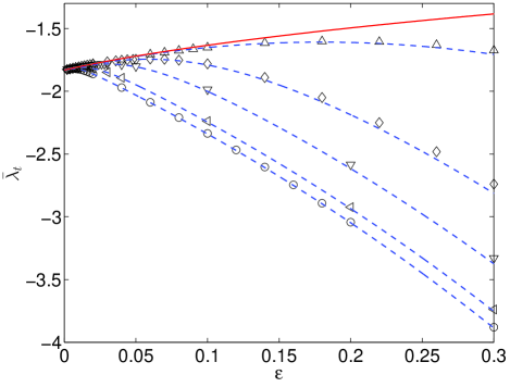
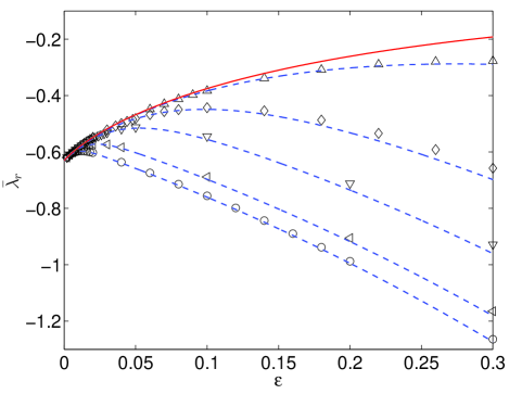
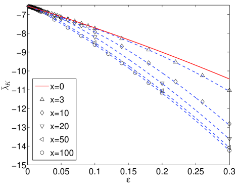
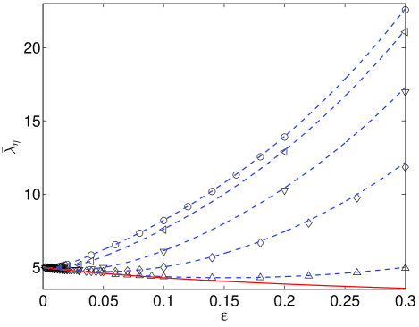
Figure 4: The two-particle virial coefficients $\bar{\lambda}(x,\epsilon)$, as functions of the shell thickness $\epsilon$, for suspensions of core-shell particles with $x=0$ (solid line), and $x=3$, $10$, $20$, $50$, $100$ (symbols), in comparison to the effective annulus model, $\bar{\lambda}^{A}_{\text{eff}}$ (dashed lines). Top: the translational and rotational self-diffusion coefficients, $\bar{\lambda}_{t}$ and $\bar{\lambda}_{r}$. Bottom: the sedimentation and high-frequency viscosity coefficients, $\bar{\lambda}_{K}$ and $\bar{\lambda}_{\eta}$.

Table 1: The annulus model: Two-particle contributions to the short-time translational and rotational self-diffusion, $\bar{\lambda}_{t}^{A}$ and $\bar{\lambda}_{r}^{A}$, sedimentation, $\bar{\lambda}_{K}^{A}$, and high-frequency viscosity, $\bar{\lambda}_{\eta}^{A}$.

$\delta$	$\bar{\lambda}_{t}^{A}$	$\bar{\lambda}_{K}^{A}$	$\bar{\lambda}_{r}^{A}$	$\bar{\lambda}_{\eta}^{A}$
0.000	-1.8315	-6.5464	-0.6305	5.0021
0.020	-1.7821	-6.7672	-0.5483	4.8123
0.040	-1.7397	-6.9943	-0.4916	4.6554
0.060	-1.7015	-7.2271	-0.4460	4.5187
0.080	-1.6664	-7.4654	-0.4079	4.3972
0.100	-1.6337	-7.7090	-0.3752	4.2877
0.120	-1.6030	-7.9578	-0.3466	4.1881
0.140	-1.5740	-8.2118	-0.3214	4.0970
0.160	-1.5465	-8.4710	-0.2990	4.0132
0.180	-1.5203	-8.7353	-0.2789	3.9357
0.200	-1.4952	-9.0048	-0.2608	3.8639
0.220	-1.4712	-9.2793	-0.2444	3.7970
0.240	-1.4481	-9.5589	-0.2294	3.7347
0.260	-1.4259	-9.8436	-0.2158	3.6765
0.280	-1.4045	-10.1334	-0.2033	3.6220
0.300	-1.3838	-10.4282	-0.1919	3.5708
0.320	-1.3638	-10.7281	-0.1813	3.5228
0.340	-1.3445	-11.0331	-0.1716	3.4777
0.360	-1.3257	-11.3430	-0.1626	3.4352
0.380	-1.3075	-11.6580	-0.1542	3.3952
0.400	-1.2898	-11.9780	-0.1465	3.3574
0.420	-1.2727	-12.3031	-0.1392	3.3217
0.440	-1.2560	-12.6332	-0.1325	3.2880
0.460	-1.2397	-12.9683	-0.1262	3.2560
0.480	-1.2239	-13.3084	-0.1203	3.2258
0.500	-1.2085	-13.6535	-0.1148	3.1972

The effective annulus intrinsic viscosity is the same as for a solid sphere,

$$\bar{[\eta]}^{A}(\delta) = \frac{5}{2}.$$ (36)

As discussed in Sec. III and illustrated in Fig. 3, the effective annulus approximation corresponds to $c=a_{\text{eff}}$, with the effective radius given by Eqs. (25)-(28).

To compare the core-shell virial coefficients $\bar{\lambda}(x,\epsilon)$ with the corresponding values for the effective annulus model, we first evaluate the effective radius $a_{\text{eff}}$ and the corresponding effective shell thickness $\epsilon_{\text{eff}}$ from Eqs. (26)-(28) and (30), then we evaluate from Table 1 the two-particle virial coefficients $\bar{\lambda}^{A}(\epsilon_{\text{eff}})$ for the annulus model, and finally perform the appropriate rescaling of the volume fraction $\phi_{a_{\text{eff}}}=4\pi na_{\text{eff}}^{3}/3$ to $\phi_{a}=4\pi na^{3}/3$ (which is used in defining $\bar{\lambda}(x,\epsilon)$ for the core-shell model),

$$\bar{\lambda}^{A}_{\text{eff}} \equiv \bar{\lambda}^{A}(\epsilon_{\text{eff}})\left(\frac{a_{\text{eff}}}{a}\right)^{\alpha},$$ (37)

with $\alpha=3$ for $\lambda_{t}$, $\lambda_{K}$, $\lambda_{r}$ and $\alpha=6$ for $\lambda_{\eta}$. The effective annulus intrinsic viscosity,

$$\bar{[\eta]}^{A}_{\text{eff}} = \frac{5}{2}\left(\frac{a_{\text{eff}}}{a}\right)^{3}.$$ (38)

V.3 The core-shell particles with thin shells

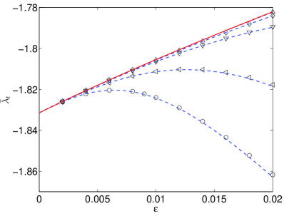
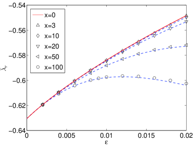
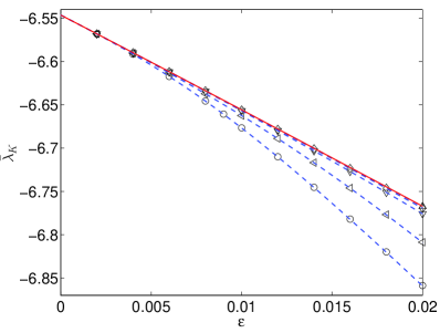
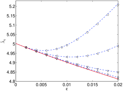
Figure 5: Unlargement of Fig. 4 for very thin shells.

Based on the previous sections, we now conclude that for core-shell particles with thin shells, the virial coefficients $\bar{[\eta]}$ and $\bar{\lambda}$ are well-approximated by the corresponding values following from the effective annulus model,

$$\bar{[\eta]}\!\approx\!\bar{[\eta]}^{A}_{\text{eff}}\hskip 7.11317pt\mbox{and}\hskip 7.11317pt\bar{\lambda}\!\approx\!\bar{\lambda}^{A}_{\text{eff}}\hskip 7.11317pt\mbox{for }\epsilon\!\rightarrow\!0,$$ (39)

with the neglected terms scaling as $\sim(x^{2}\epsilon^{4})$. With the use of the expressions from Appendix B, the two-particle virial coefficients $\bar{\lambda}(x,\epsilon)$ have been evaluated. In Figs. 4 and 5, the values of $\bar{\lambda}$ for the core-shell particles are compared with their analogs $\bar{\lambda}^{A}_{\text{eff}}$ for the effective annulus model. It is clear that the effective annulus approximation is very accurate, with the range of validity even wider than it could be expected from the thin-shell expansion (13).

VI Conclusions

There are two main conlcusions following from this work. The first one is that for core-shell particles with thin shells, characterized by large permeabilities, the effective annulus model very accurately approximates the self-diffusion, sedimentation and viscosity coefficients of core-shell suspensions. This general statement has been derived from the asymptotic expansion of the scattering coefficients in the thin-shell limit ($a,\kappa=\mbox{const},\epsilon\rightarrow 0$), and explicitly illustrated by evaluation of the two-particle virial contributions to the transport coefficients, $\bar{\lambda}(x,\epsilon)$, which are shown in Fig. 4. Actually, the range of validity of the effective annulus approximation, $\bar{\lambda}=\bar{\lambda}^{A}_{\text{eff}}[1+{\cal O}(\epsilon^{4})]$, with the neglected terms $\sim x^{2}\epsilon^{4}$, extends beyond the case of $x^{2}\epsilon^{4}\lesssim 1$.

The second important outcome is that the effective annulus model for suspensions of core-shell particles with highly permeable shells is much more accurate than just the effective hard-core approximation, in which the particle shells are totally neglected (as completely permeable and overlapping with each other). This effect is explicitly shown on the level of two-particle interactions. Large differences between the accurate effective annulus approximation to $\bar{\lambda}_{r}$, and the corresponding predictions of the imprecise effective hard-sphere model are illustrated in Fig. 6.

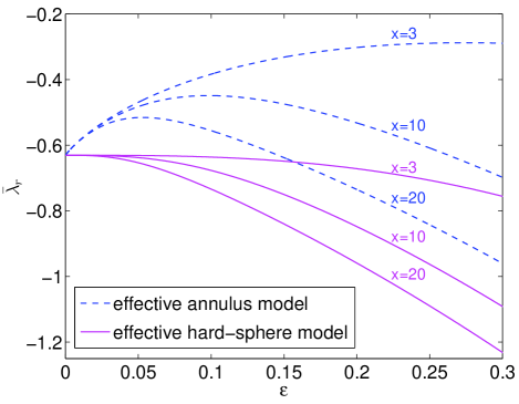
Figure 6: For very permeable shells, the effective hard-sphere model is not accurate, in contrast to the effective annulus model, compare with the right upper panel of Fig. 4.

The comparison of the accuracy of both models applied to $\bar{\lambda}(x\!\!=\!\!10,\epsilon\!\!=\!\!0.3)$ is performed in Table 2. For $x\!\lesssim\!10$ and $\epsilon\!\gtrsim\!0.3$, the effective hard-core model is not adequate, especially for the rotational self-diffusion.

Table 2: Relative accuracy $\Delta\bar{\lambda}$ of a virial coefficient $\bar{\lambda}$ in the effective annulus and effective hard sphere models, for $\epsilon\!\!=\!\!0.3$ and $x\!\!=\!\!10$.

	$\Delta\bar{\lambda}_{t}$	$\Delta\bar{\lambda}_{K}$	$\Delta\bar{\lambda}_{r}$	$\Delta\bar{\lambda}_{\eta}$
effective annulus model	1%	0.2%	3%	2%
effective hard sphere model	14%	13%	66%	19%

The main result of this paper is to derive, in the thin-shell limit ($a,\kappa=\mbox{const},\epsilon\rightarrow 0$), validity of the effective annulus approximation to the core-shell systems, and to demonstrate how to use table 1 of the annulus values to determine accurately the core-shell transport coefficients in the semi-dilute regime (and for relatively thin shells), knowing the geometrical and the hydrodynamical radii of a core shell-particle.

Appendix A Scattering coefficients

The single-particle friction operator ${\bf Z}_{0}$ is expressed in terms of the scattering coefficients by the following relation,

$$Z_{0}(ilm\sigma,il^{\prime}m^{\prime}\sigma^{\prime})=\delta_{ll^{\prime}}\delta_{mm^{\prime}}\eta(2l\!+\!1)\!\left[\!\!\begin{array}[]{ccc}\displaystyle\frac{2l(2l\!-\!1)}{l\!+\!1}A_{l0}&0&(2l\!-\!1)(2l\!+\!1)A_{l2}\\ \\ 0&\!l(l\!+\!1)A_{l1}\!&0\\ \\ (2l\!-\!1)(2l\!+\!1)A_{l2}&0&\displaystyle\frac{(l\!+\!1)(2l\!+\!1)^{2}(2l\!+\!3)}{2l}B_{l2}\end{array}\!\!\right],\!\!\!\!\!\!\!\!\!\!\!\!\!$$ (45)

and

$$\hat{\bf Z}_{0}={\bf Z}_{0}-{\bf Z}_{0}\,\mbox{\boldmath$\mu$}_{0}\,{\bf Z}_{0},$$ (47)

with the only non-zero matrix elements of $\mbox{\boldmath$\mu$}_{0}$ for $l=1$ and $\sigma=0,1$,

$$\mu_{0}(i1m\sigma,i1m^{\prime}\sigma) = [Z_{0}(i1m\sigma,i1m^{\prime}\sigma)]^{-1}.$$ (48)

The explicit (lengthy) expressions for the scattering coefficients $A_{l\sigma}(x,a,b)$ for core-shell particles have been derived in Ref. Cichocki_Felderhof:09 . Their asymptotic expansion in the thin-shell limit (13) is given in Sec. III. Below, we list the scattering coefficients for hard spheres of radius $a$,

$$A_{l0}=\frac{2l+1}{2}a^{2l-1},\hskip 22.76228ptA_{l1}=a^{2l+1},$$

$$A_{l2}=\frac{2l+3}{2}a^{2l+1},\hskip 22.76228ptB_{l2}=\frac{2l+1}{2}a^{2l+3}.\hskip 25.6073pt$$ (49)

Appendix B Two-particle virial coefficients

In this Appendix, we derive expressions for the two-particle virial coefficients ${\bar{\lambda}}(x,\epsilon)$ of the core-shell suspensions. In the limit of $\kappa$=0 (i.e. $x$=0), the annulus model with the inner radius $c=a$ is recovered.

We introduce dimensionless interparticle distance, $R$=$r/2a$. The pair distribution function has the form,

$$g_{0}(R) = \left\{\begin{array}[]{ll}0&\mbox{ for }\;R\leq 1+\epsilon,\\ 1&\mbox{ for }\;R>1+\epsilon.\end{array}\right.$$ (52)

which corresponds to the no-overlap condition at the larger shell radius $b=a(1+\epsilon)$.

The two-particle virial coefficients are evaluated from the following expressions,

$${\bar{\lambda}}_{t}(x,\epsilon)\!\! = \!\!8\int_{1+\epsilon}^{+\infty}J_{t}(R)R^{2}dR,$$ (53)

$${\bar{\lambda}}_{K}(x,\epsilon)\!\! = \!\!\frac{2}{5a^{3}}A_{12}-\frac{4}{a}A_{10}(1+\epsilon)^{2}$$ (54)

$$+ 8\int_{1+\epsilon}^{+\infty}J_{K}(R)R^{2}dR,$$

$${\bar{\lambda}}_{r}(x,\epsilon)\!\! = \!\!8\int_{1+\epsilon}^{+\infty}J_{r}(R)R^{2}dR,$$ (55)

$$\bar{\lambda}_{\eta}(x,\epsilon)\!\! = \!\!\frac{2}{5}\bar{[\eta]}^{2}+24\bar{[\eta]}\int_{1+\epsilon}^{\infty}J_{\eta}(R)R^{2}dR,\hskip 14.22636pt$$ (56)

where

$$J_{t}(R)\!\! = \!\!\frac{1}{\mu_{0}^{t}}\mbox{Tr}\,\bm{\mu}_{11}^{tt(2)}(\mathbf{R}),$$ (57)

$$J_{K}(R)\!\! = \!\!\frac{1}{\mu_{0}^{t}}\mbox{Tr}\left[\bm{\mu}_{11}^{tt(2)}(\mathbf{R})+\bm{\mu}_{12}^{tt(2)}(\mathbf{R})-\mathbf{T}_{0}(\mathbf{R)}\right]\!,\hskip 17.07182pt$$ (58)

$$J_{r}(R)\!\! = \!\!\frac{1}{\mu_{0}^{r}}\mbox{Tr}\,\bm{\mu}_{11}^{rr(2)}(\mathbf{R}),$$ (59)

$$J_{\eta}(R)\!\! = \!\!\frac{1}{5\mu_{0}^{d}}\left[{\mu}^{dd(2)}_{11,\alpha\beta\beta\alpha}({\bf R})+{\mu}^{dd(2)}_{12,\alpha\beta\beta\alpha}({\bf R})\right]\!,\hskip 14.22636pt$$ (60)

with the single particle dipole mobility $\mu_{0}^{d}$ given by Eqs. (7) and (10). In the above expressions, Tr denotes the trace operation, and

$$\mathbf{T}_{0}(\mathbf{R)=}\frac{\mathbf{1+}\widehat{\mathbf{R}}\widehat{\mathbf{R}}}{8\pi\eta_{0}R},$$ (61)

is the Oseen tensor, with $\widehat{\mathbf{R}}=\mathbf{R/}R$. All the mobility coefficients, the associated functions $J$ and the scattering coefficients $A_{l\sigma}$ in Eqs. (53)-(60) refer to the core-shell particles.

References

- (1) A. Kasper, E. Bartsch and H. Sillescu, Langmuir 14, 5004 (1998).
- (2) M. H. G. Duits, P. A. Nommensen, D. van den Ende, and J. Mellema, Colloids Surf. A 183-185, 335 (2001).
- (3) G. Petekidis, J. Gapiński, P. Seymour, J. S. van Duijneveldt, D. Vlassopoulos and G. Fytas, Phys. Rev. E 69, 042401 (2004).
- (4) M. Zackrisson, A. Stradner, P. Schurtenberger and J. Bergenholtz, Langmuir 21, 10835 (2005).
- (5) M. Zackrisson, A. Stradner, P. Schurtenberger and J. Bergenholtz, Phys. Rev. E 73, 011408 (2006).
- (6) M. Siebenbürger , M. Fuchs and M. Ballauff, Soft Matter, 8, 4014(2012).
- (7) G. C. Abade, B. Cichocki, M. L. Ekiel-Jeżewska, G. Nägele, and E. Wajnryb, J. Chem. Phys. 136, 104902 (2012).
- (8) M. Zackrisson, J. Bergenholtz, Colloids Surf. A, 225, 119 (2003).
- (9) B. Cichocki and B. U. Felderhof, J. Chem. Phys. 130, 164712 (2009).
- (10) J. Masliyah, G. Neale, K. Malysa, and T.G.M. van de Ven, Chem. Eng. Science 42, 245 (1987).
- (11) S. B. Chen and X. Ye, J. Colloid Interface Sci. 221, 50 (2000).
- (12) G. C. Abade, B. Cichocki, M. L. Ekiel-Jeżewska, G. Nägele, and E. Wajnryb, J. Chem. Phys. 133, 084906 (2010).
- (13) S. Kim and S. J. Karrila. Microhydrodynamics. Principles and Selected Applications. Butterworth-Heinemann, London, 1991.
- (14) J. Happel and H. Brenner. Low Reynolds Number Hydrodynamics. Martinus Nijhoff, Dordrecht, 1986.
- (15) H. C. Brinkman, Appl. Scient. Res. A1 27, 81 (1947).
- (16) P. Debye and A. M. Bueche, J. Chem. Phys. 16, 573 (1948).
- (17) B. Cichocki, B. U. Felderhof, K. Hinsen, E. Wajnryb, and J. Bławzdziewicz, J. Chem. Phys. 100, 3780 (1994).
- (18) M. L. Ekiel-Jeżewska and E. Wajnryb, in Theoretical Methods for Micro Scale Viscous Flows, edited by F. Feuillebois and A. Sellier, Transworld Research Network, Kerala, 2009.
- (19) B. Cichocki, M. L. Ekiel-Jeżewska and E. Wajnryb, J. Chem. Phys. 111, 3265 (1999).
- (20) B. Cichocki, M. L. Ekiel-Jeżewska, P. Szymczak and E. Wajnryb, J. Chem. Phys. 117, 1231 (2002).
- (21) B. Cichocki, M.L. Ekiel-Jeżewska and E. Wajnryb, J. Chem. Phys. 119, 606 (2003).
- (22) G. C. Abade, B. Cichocki, M. L. Ekiel-Jeżewska, G. Nägele, and E. Wajnryb, J. Chem. Phys. 132, 014503 (2010).
- (23) B. Cichocki, B. U. Felderhof and R. Schmitz, PhysicoChemical Hydrodynamics 10, 383 (1988).
- (24) H. Lamb, Hydrodynamics, Cambridge University Press, Cambridge, 1993.
- (25) B. Cichocki and B. U. Felderhof, J. Chem. Phys. 94, 556 (1991).