Abstract

As a canonical and generally covariant gauge theory, loop quantum gravity requires special techniques to derive effective actions or equations. If the proper constructions are taken into account, the theory, in spite of considerable ambiguities at the dynamical level, allows for a meaningful phenomenology to be developed, by which it becomes falsifiable. The tradiational problems plaguing canonical quantum-gravity theories, such as the anomaly issue or the problem of time, can be overcome or are irrelevant at the effective level, resulting in consistent means of physical evaluations. This contribution presents aspects of canonical equations and related notions of (deformed) space-time structures and discusses implications in loop quantum gravity, such as signature change at high density from holonomy corrections, and falsifiability thanks to inverse-triad corrections.

1 Introduction

Loop quantum gravity [1, 2, 3] is a proposal for a canonical quantization of general relativity. By a careful use of basic variables suitable for a quantum representation independent of auxiliary metric or causal structures, it has shed light on several aspects of the quantum geometry of space. The dynamics of the theory, however, remains poorly controlled, and therefore it is not clear what structure of quantum space-time it implies. Dynamical operators are subject to quantum ambiguities, and their evaluation is still plagued by long-standing conceptual problems of canonical quantum gravity, most famously the problem of time [4, 5, 6].

That much-needed progress especially on the last-mentioned problem is lacking is illustrated for instance by the proliferating use of “deparameterized” quantum theories, in which the time variable is fixed once and for all (as a matter degree of freedom rather than a coordinate). The space-time gauge is partially fixed, even though one set out to derive properties of quantum space-time. Such time-fixed systems have been seriously proposed not just as toy models but even as complete quantum theories of gravity (see e.g. [7]). With these attempts, one no longer aims at gaining control over quantum space-time and its physical effects, for which one would have to show that quantum observables are independent of the choice of time, be it an internal matter clock or a coordinate; no such results of independence have been provided in deparameterized models.

With problems like these still outstanding, it remains questionable whether the theory can be considered as fundamental. (Of course, this is not to say that the theory could not achieve fundamental status with further, significant progress.) Nevertheless, the theory’s results regarding the quantum geometry of space and background independence may still be of physical interest, provided they can manifest themselves in sufficiently characteristic ways on the typical scales of gravitational phenomena, far removed from the microscopic Planck scale. This is the realm of effective theory, a powerful viewpoint in many examples (not only) of high-energy phenomena, so also in loop quantum gravity as laid out in this contribution.

The dynamical problems of loop quantum gravity are not specific to this particular approach but have a general origin in relativistic properties of space-time. Generally covariant theories, such as general relativity, have complicated gauge structures (coordinate transformations, or hypersurface deformations) that can best be addressed with canonical techniques. (For canonical methods in gravity, see [8].) In such settings they show their troubling face most directly, but they also sneak through other approaches, for instance those using path integrals or spin foams where finding the correct integration measure is a related problem. These issues require special care, new methods of quantum field theory and semiclassical or effective descriptions. Here we present an overview of the following techniques, suitable for physical evaluations of the theory: (i) A canonical derivation of effective equations for quantum dynamics, and (ii) a discussion of general covariance in quantum gravity and deformed space-time structures. By bringing these parts together, an effective theory of loop quantum gravity is obtained.

2 Effective theories

In quantum theory, every local classical degree of freedom, $(q,p)$ in canonical form, amounts to infinitely many quantum degrees of freedom — expectation values $\langle\hat{q}\rangle$, $\langle\hat{p}\rangle$, fluctuations (squared) $\langle\hat{q}^{2}\rangle-\langle\hat{q}\rangle^{2}$, and so on with higher powers. An effective theory, in general terms, aims to describe some properties of quantum theory by interactions of finitely many local degrees of freedom. For instance, if we keep only the expectation values, we have the classical limit. Expectation values together with fluctuations, taking values near saturation of the uncertainty relation, provide the first-order approximation in $\hbar$. The higher the $\hbar$-order, the more degrees of freedom must be considered (related but not identical to higher time derivatives). In a formal limit including the order $\hbar^{\infty}$, we are back at quantum theory, but in perturbative guise. Some subtle effects may be missed, for instance different inequivalent self-adjoint extensions of Hamiltonians. But many dynamical properties independent of subtleties can be derived conveniently using effective theory. One may therefore hope that some of the technical and conceptual problems of quantum gravity or quantum cosmology can be simplified as well, and this hope is indeed borne out.

2.1 Quantum phase space

Like most other questions, the idea of effective theories can easily be illustrated by the harmonic oscillator, with a quadratic Hamiltonian $\hat{H}=\frac{1}{2m}\hat{p}^{2}+\frac{1}{2}m\omega^{2}\hat{q}^{2}$ for canonical commutation relations $[\hat{q},\hat{p}]=i\hbar$. (However, harmonic-oscillator results should be taken with a grain of salt when it comes to general behavior, as we will see in the present context as well.) For an effective theory in terms of expectation values, we compute equations of motion

$$\frac{{\rm d}}{{\rm d}t}\langle\hat{q}\rangle=\frac{1}{i\hbar}\langle[\hat{q},\hat{H}]\rangle=\frac{1}{m}\langle\hat{p}\rangle\quad,\quad\frac{{\rm d}}{{\rm d}t}\langle\hat{p}\rangle=\frac{1}{i\hbar}\langle[\hat{p},\hat{H}]\rangle=-m\omega^{2}\langle\hat{q}\rangle$$

which can be solved directly. Although they amount to just the classical equations for $q$ and $p$, their solutions determine exact quantum properties.

To go beyond the classical order free of $\hbar$-dependent terms, we can use the same type of equations of motion to derive dynamical laws for fluctuations $(\Delta O)^{2}=\langle\hat{O}^{2}\rangle-\langle\hat{O}\rangle^{2}$ of $q$ and $p$ and, as it turns out to be necessary, the covariance. $C_{qp}=\frac{1}{2}\langle\hat{q}\hat{p}+\hat{p}\hat{q}\rangle-\langle\hat{q}\rangle\langle\hat{p}\rangle$. These variables provide all degrees of freedom to second order, with expectation values of quadratic functions of the basic operators. In a semiclassical state, the values are of the order $\hbar$, as one can verify explicitly for a Gaussian.

Dynamically, we have the equations

$$\frac{{\rm d}}{{\rm d}t}(\Delta q)^{2} = \frac{\langle[\hat{q}^{2},\hat{H}]\rangle}{i\hbar}-2\langle\hat{q}\rangle\frac{{\rm d}\langle\hat{q}\rangle}{{\rm d}t}=\frac{2}{m}C_{qp}$$ (1)

$$\frac{{\rm d}}{{\rm d}t}C_{qp} = -m\omega^{2}(\Delta q)^{2}+\frac{1}{m}(\Delta p)^{2}$$ (2)

$$\frac{{\rm d}}{{\rm d}t}(\Delta p)^{2} = -2m\omega^{2}C_{qp}$$ (3)

and we should also restrict the variables for them to correspond to a true state: they are subject to the (generalized) uncertainty relation

$$(\Delta q)^{2}(\Delta p)^{2}-C_{qp}^{2}\geq\frac{\hbar^{2}}{4}\,.$$ (4)

Just like expectation-value equations, these second-order equations are linear and can easily be solved, providing non-classical information about quantum states. Stationary states, for instance, require $C_{qp}=0$ for the variables to remain constant in time, together with $\Delta p=m\omega\Delta q$ from (2). They satisfy the uncertainty relation if $\Delta q\geq\sqrt{\hbar/2m\omega}$. The uncertainty relation is saturated for $\Delta q=\sqrt{\hbar/2m\omega}$, in which we find the correct fluctuations of the harmonic-oscillator ground state. More general squeezed coherent states with $C_{qp}\not=0$, still saturating the generalized uncertainty relation, have time-dependent fluctuations, such as a spread oscillating oscillating with frequency $2\omega$; see Fig. 1. One can explicitly solve (1)–(3) for the position fluctuation

$$(\Delta q)^{2}(t)=\frac{C_{0}}{m\omega}\sin(2\omega t)+\frac{1}{2}(Q_{0}-P_{0}/m^{2}\omega^{2})\cos(2\omega t)+\frac{1}{2}(Q_{0}+P_{0}/m^{2}\omega^{2})$$ (5)

with $C_{0}$, $Q_{0}$ and $P_{0}$ the initial values of $C_{qp}$, $(\Delta q)^{2}$ and $(\Delta p)^{2}$, respectively. With similar solutions for $(\Delta p)^{2}(t)$ and $C_{qp}(t)$, one sees that $(\Delta q)^{2}(\Delta p)^{2}-C_{qp}^{2}$ is constant: the states are dynamical coherent states.

Figure 1: Dynamical coherent states of the harmonic oscillator, uncorrelated with constant fluctuations (solid) or correlated with oscillating fluctuations (dashed). All states spread around the same time-dependent expectation value $q(t)$ (central line) but differ in the dynamics of their position fluctuations (lines around the mean).

In this system, exact quantum properties follow from finitely many variables. A more complicated but still tractable model is the “relativistic” harmonic oscillator, in which the energy $\hat{E}^{2}=\frac{1}{2m}\hat{p}^{2}+\frac{1}{2}m\omega^{2}\hat{q}^{2}$, compared to the standard harmonic oscillator, enters quadratically [9]. As Fig. 2 shows, simple properties of an initial coherent state become much more complicated as time goes on, and deviations from classical trajectories occur. This form of quantum back-reaction — the influence of the shape of a state on the trajectory — happens generically in quantum systems, while the strict decoupling of quantum variables and expectation values is special to the harmonic oscillator and a few other systems.

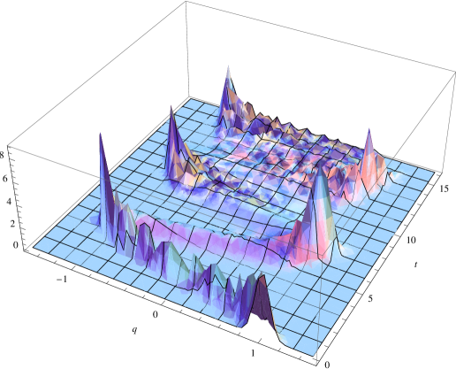
Figure 2: A wave function subject to the dynamics of a “relativistic” harmonic oscillator, with quantum back-reaction. Starting as a Gaussian (front), the state for some time follows the classical oscillating trajectory but spreads out and eventually shows no clear trajectory [9].

For controlled deviations from harmonicity, we look at an anharmonic oscillator with non-quadratic Hamiltonian

$$\hat{H}=\frac{1}{2m}\hat{p}^{2}+V(\hat{q})=\frac{1}{2m}\hat{p}^{2}+\frac{1}{2}m\omega^{2}\hat{q}^{2}+\frac{1}{3}\lambda\hat{q}^{3}\,.$$

The cubic term could be seen as a perturbation for $\lambda$ sufficiently small, provided $q$ does not grow too large. Now, equations of motion read

$$\frac{{\rm d}}{{\rm d}t}\langle\hat{q}\rangle=\frac{1}{m}\langle\hat{p}\rangle\quad,\quad\frac{{\rm d}}{{\rm d}t}\langle\hat{p}\rangle=-m\omega^{2}\langle\hat{q}\rangle-\lambda\langle\hat{q}\rangle^{2}-(\Delta q)^{2}=-V^{\prime}(\langle\hat{q}\rangle)-\lambda(\Delta q)^{2}\,,$$

coupling expectation values to the position fluctuation. (Similar equations for $\hbar\to 0$ have been used in [10] to prove that quantum mechanics has the correct classical limit.) The position fluctuation, in turn, obeys

$$\frac{{\rm d}}{{\rm d}t}(\Delta q)^{2}=\frac{2}{m}C_{qp}\quad,\quad\frac{{\rm d}}{{\rm d}t}C_{qp}=\frac{1}{m}(\Delta p)^{2}-m\omega^{2}(\Delta q)^{2}+6\lambda\langle\hat{q}\rangle(\Delta q)^{2}+3\lambda G^{0,3}$$

and depends, via the evolution equation of $C_{qp}$, on a third-order moment $G^{0,3}=\langle(\hat{q}-\langle\hat{q}\rangle)^{3}\rangle$ (called skewness). Proceeding in this way, computing an equation of motion for $G^{0,3}$ and so on, shows that infinitely many variables are coupled to one another and to expectation values.

For a systematic formulation, we use, following [11, 12], the quantum phase space of classical variables $q=\langle\hat{q}\rangle$ and $p=\langle\hat{p}\rangle$ together with the moments

$$G^{a,n}:=\langle(\hat{q}-\langle\hat{q}\rangle)^{n-a}(\hat{p}-\langle\hat{p}\rangle)^{a}\rangle_{\rm Weyl}$$ (6)

for $n\geq 2$, $a=0,\ldots,n$. (The subscript “Weyl” indicates that all operator products are Weyl ordered before taking the expectation value, averaging over all possible orderings.) For these variables we have Poisson brackets

$$\{\langle\hat{A}\rangle,\langle\hat{B}\rangle\}=\frac{\langle[\hat{A},\hat{B}]\rangle}{i\hbar}$$ (7)

extended by imposing the Leibniz rule to products of expectation values, as they appear in moments. This general definition implies $\{q,p\}=1$, $\{q,G^{a,n}\}=0=\{p,G^{a,n}\}$ and a rather complicated (but explicitly known) relation for $\{G^{a,n},G^{b,m}\}$ [11, 13].

2.2 Effective dynamics

Evolution on the quantum phase space is determined by the quantum Hamiltonian $H_{Q}(\langle\cdot\rangle,G^{\cdot,\cdot})=\langle\hat{H}\rangle_{\langle\cdot\rangle,G^{\cdot,\cdot}}$, defined as a function of expectation values and moments characterizing a state used to compute the expectation value. The dynamical flow of the quantum Hamiltonian couples expectation values and moments: the law

$$\frac{{\rm d}\langle\hat{O}\rangle}{{\rm d}t}=\frac{\langle[\hat{O},\hat{H}]\rangle}{i\hbar}=\{\langle\hat{O}\rangle,\langle\hat{H}\rangle\}$$ (8)

in general contains product terms multiplying expectation values and moments. In this systematic way, quantum back-reaction is implemented.

A well-studied example illustrating all important features is the general anharmonic oscillator, with classical Hamiltonian $H=\frac{1}{2m}p^{2}+\frac{1}{2}m\omega^{2}q^{2}+U(q)$. If we first introduce dimensionless variables $\tilde{G}^{a,n}=\hbar^{-n/2}(m\omega)^{n/2-a}G^{a,n}$, we can compute the quantum Hamiltonian $H_{Q}:=\langle\hat{H}\rangle$ that enters the Poisson bracket in (8), exhibiting all quantum corrections with explicit factors of $\hbar$. By Taylor expansion, we have

$$H_{Q} = \langle H(\hat{q},\hat{p})\rangle=\langle H(\langle\hat{q}\rangle+(\hat{q}-\langle\hat{q}\rangle),\langle\hat{p}\rangle+(\hat{p}-\langle\hat{p}\rangle))\rangle$$

$$= \frac{1}{2m}\langle\hat{p}\rangle^{2}+\frac{1}{2}m\omega^{2}\langle\hat{q}\rangle^{2}+U(\langle\hat{q}\rangle)+\frac{\hbar\omega}{2}(\tilde{G}^{0,2}+\tilde{G}^{2,2})+\sum_{n>2}\frac{1}{n!}\left(\frac{\hbar}{m\omega}\right)^{n/2}U^{(n)}(\langle\hat{q}\rangle)\tilde{G}^{0,n}$$

with the zero-point energy $\frac{1}{2}\hbar\omega(\tilde{G}^{0,2}+\tilde{G}^{2,2})$ and a whole series of coupling terms. The series, in general, is asymptotic, as usual for semiclassical expansions. If it is truncated to a finite sum up to $n_{\rm max}$, we obtain the semiclassical approximation of order $n_{\rm max}$.

The quantum Hamiltonian $H_{Q}$ generates Hamiltonian equations of motion $\dot{f}=\{f,H_{Q}\}$ on quantum phase space according to (8): from [11],

$$\dot{\langle\hat{q}\rangle} = \frac{\langle\hat{p}\rangle}{m}$$ (10)

$$\dot{\langle\hat{p}\rangle} = -m\omega^{2}\langle\hat{q}\rangle-U^{\prime}(\langle\hat{q}\rangle)-\sum_{n}\frac{1}{n!}\left(\frac{\hbar}{m\omega}\right)^{n/2}U^{(n+1)}(\langle\hat{q}\rangle)\tilde{G}^{0,n}$$ (11)

$$\dot{\tilde{G}}{}^{a,n} = -a\omega\tilde{G}^{a-1,n}+(n-a)\omega\tilde{G}^{a+1,n}-a\frac{U^{\prime\prime}(\langle\hat{q}\rangle)}{m\omega}\tilde{G}^{a-1,n}$$

$$+\frac{\sqrt{\hbar}aU^{\prime\prime\prime}(\langle\hat{q}\rangle)}{2(m\omega)^{3/2}}\tilde{G}^{a-1,n-1}\tilde{G}^{0,2}+\frac{\hbar aU^{{}^{\prime\prime\prime\prime}}(\langle\hat{q}\rangle)}{3!(m\omega)^{2}}\tilde{G}^{a-1,n-1}\tilde{G}^{0,3}$$

$$-\frac{a}{2}\left(\frac{\sqrt{\hbar}U^{\prime\prime\prime}(\langle\hat{q}\rangle)}{(m\omega)^{3/2}}\tilde{G}^{a-1,n+1}+\frac{\hbar U^{{}^{\prime\prime\prime\prime}}(\langle\hat{q}\rangle)}{3(m\omega)^{2}}\tilde{G}^{a-1,n+2}\right)+\cdots$$

with infinitely many coupled equations for infinitely many variables, clearly a system that in this generality is difficult to manage. Nevertheless, we can see some general properties:

• Quantum corrections arise from back-reaction of fluctuations and higher moments (loop corrections in the language of quantum field theory) unless the system is harmonic with $U(q)=0$ (or “free”).

• State properties such as fluctuations are computed if we solve our equations, starting from initial conditions (the interacting vacuum). There is no need to assume properties of dynamical semiclassical states, which in other schemes are often based on ad-hoc choices such as Gaussians as the simplest peaked states.

• The procedure is manageable if a free system is available as perturbative basis. The most general form of such a system is one with a linear dynamical algebra $[\hat{J}_{i},\hat{J}_{j}]=\sum_{k}C_{ij}{}^{k}\hat{J}_{k}$ for a complete set of basic operators $\hat{J}_{i}$ that includes the Hamiltonian $\hat{H}$. With canonical basic variables, $\hat{H}$ must be quadratic for this condition to be realized. More general, non-canonical examples are known in quantum cosmology [14].

Figure 3: Position and momentum expectation values for the system shown in Fig. 2. Quantum back-reaction is captured to leading order in a semiclassical expansion as shown by the dashed curve [9]. Unlike the classical orbit (dotted), the effective one follows the quantum corrections seen in the expectation value of the state starting semiclassically as in Fig. 2. (Initial values for the effective orbit are chosen so that they agree with expectation values and moments of the initial Gaussian profile of the semiclassical wave function.)

Figure 4: The uncertainty product $4\hbar^{-2}\left((\Delta q)^{2}(\Delta p)^{2}-C_{qp}^{2}\right)$, bounded from below by one according to (4), increases, showing that the state used in Figs. 2 and 3 evolves away from semiclassicality [9].

Figure 5: Relative second-order moments $\Delta(q^{a}p^{b})_{\rm rel}=\Delta(q^{a}p^{b})/\langle\hat{q}\rangle^{a}\langle\hat{p}\rangle^{b}$ of the state shown in Figs. 2 and 3, computed by effective equations (dashed) and from an evolving wave function (solid). When moments grow too large, surpassing the threshold indicated by the horizontal line, the semiclassical approximation to the order used breaks down [9].

Figure 6: Long-term plot of the relative skewness $\Delta(q^{3})_{\rm rel}=\Delta(q^{3})/\langle\hat{q}\rangle^{3}$ for a wave function shown in Fig. 2. The state rapidly evolves away from a Gaussian, which would have zero skewness. Even though small values may again be attained later, the full state, characterized by infinitely many moments, may be far from being Gaussian [9].

\psfrag{ttdiv}{$t$}\psfrag{Lambda}{}\psfrag{LogGijPV}{even moments}\includegraphics[height=126.47249pt]{0ii0iieven_l104}

\psfrag{ttdiv}{$t$}\psfrag{Lambda}{}\psfrag{LogGijPV}{even moments}\psfrag{ttdiv}{$t$}\psfrag{LogGij}{$\log(\mbox{odd moments})$}\psfrag{Lambda}{}\includegraphics[height=126.47249pt]{ijoddigreaterj_l108}

Figure 7: Moments up to order 10, even at left and odd at right, for a cosmological model with a positive cosmological constant [13]. (Moments are rescaled by powers of $\hbar$ depending on their order.) The state remains semiclassical for some time, as indicated by the hierarchy shown by the moments of different orders. However, although the initial state is Gaussian, with vanishing odd-order moments, the evolving state has a different, more complicated shape as shown by the non-zero odd-order moments on the right. Still, a dynamical hierarchy of the moments builds up as the non-Gaussian state is evolved.

Truncated to finite semiclassical order, the equations for expectation values and moments are amenable to detailed numerical analysis; see Figs. 3–7 for examples. In many cases they can also be solved analytically, at least if additional approximations are used to decouple equations. An interesting expansion is obtained when the semiclassical approximation is combined with an adiabatic one for the moments, in which case one implements a derivative expansion.

We perform the adiabatic approximation by introducing a new (unphysical) parameter $\lambda$, rescaling ${\rm d}/{\rm d}t$ to $\lambda{\rm d}/{\rm d}t$ in moment equations (2.2) and expanding $G^{a,n}=\sum_{e}G_{e}^{a,n}\lambda^{e}$ [11]. We then solve equations order by order in $\lambda$, thereby implementing the assumption of slow motion of the moments. In the end, after the system has been solved, we set $\lambda=1$ as required to recover the original equations. There is no guarantee that $\lambda=1$ lies within the radius of convergence of the expansion. Nevertheless, this form of the adiabatic expansion provides a systematic way to arrive at a derivative expansion: higher orders in $\lambda$ introduce higher time derivatives [15].

To first order in $\hbar$ and zeroth in $\lambda$ we already obtain interesting corrections. From (2.2), we then have the equation

$$0=\omega\left((n-a)G_{0}^{a+1,n}-a\left(1+\frac{U^{\prime\prime}(\langle\hat{q}\rangle)}{m\omega^{2}}\right)G_{0}^{a-1,n}\right)$$

for moments, which is algebraic instead of differential and has the general solution

$$G_{0}^{a,n}={n/2\choose a/2}{n\choose a}^{-1}\left(1+\frac{U^{\prime\prime}(\langle\hat{q}\rangle)}{m\omega^{2}}\right)^{a/2}G^{0,n}_{0}$$ (13)

for even $a$ and $n$. To this order, $G_{0}^{0,n}$ remains free.

To first order in $\lambda$, we must solve

$$(n-a)G_{1}^{a+1,n}-a\left(1+\frac{U^{\prime\prime}(\langle\hat{q}\rangle)}{m\omega^{2}}\right)G_{1}^{a-1,n}=\frac{1}{\omega}\dot{G}_{0}^{a,n}$$

for $G_{1}^{a,n}$, but the equation also implies

$$\sum_{a\>{\rm even}}{n/2\choose a/2}\left(1+\frac{U^{\prime\prime}(\langle\hat{q}\rangle)}{m\omega^{2}}\right)^{(n-a)/2}\dot{G}_{0}^{a,n}=0$$

as a condition on moments (13) of zeroth order in $\lambda$. They must then be of the form $G^{0,n}_{0}=C_{n}(1+U^{\prime\prime}(\langle\hat{q}\rangle)/m\omega^{2})^{-n/4}$ with constants $C_{n}$. At this stage, all equations relevant to this order have been implemented. The remaining freedom, the $C_{n}$, parameterize the choice of specific states used. We have solved equations of motion (2.2) for moments, corresponding to an evolving state starting with some initial wave function. The initial state so far has not been restricted, and therefore there must be free parameters left in our solutions of moments, exactly the constants $C_{n}$. In the anharmonic case, we may fix the constants by stating that the harmonic limit, $U(q)=0$, should bring us to the known moments of some state of the harmonic oscillator, such as the ground state with $C_{n}=2^{-n}n!/(n/2)!$. Using these values and inserting all solutions in our equations of motion for expectation values, we obtain the zeroth adiabatic-order correction [11]

$$\dot{p} = -m\omega^{2}q-U^{\prime}(q)-\frac{\hbar}{2m\omega}U^{\prime\prime\prime}(q)G^{0,2}+\cdots$$ (14)

$$= -m\omega^{2}q-U^{\prime}(q)-\frac{\hbar}{4m\omega}\frac{U^{\prime\prime\prime}(q)}{\sqrt{1+U^{\prime\prime}(q)/m\omega^{2}}}+\cdots\,.$$

For comparison, we also mention the second adiabatic order whose derivation is more lengthy [11]. As a second-order equation of motion, the canonical effective description

$$\left(m+\frac{\hbar U^{\prime\prime\prime}(q)^{2}}{32m^{2}\omega^{5}\left(1+U^{\prime\prime}(q)/m\omega^{2}\right)^{5/2}}\right)\ddot{q}$$

$$+\frac{\hbar\dot{q}^{2}\left(4m\omega^{2}U^{\prime\prime\prime}(q)U^{\prime\prime\prime\prime}(q)\left(1+U^{\prime\prime}(q)/m\omega^{2}\right)-5U^{\prime\prime\prime}(q)^{3}\right)}{128m^{3}\omega^{7}\left(1+U^{\prime\prime}(q)/m\omega^{2}\right)^{7/2}}$$

$$+m\omega^{2}q+U^{\prime}(q)+\frac{\hbar U^{\prime\prime\prime}(q)}{4m\omega\left(1+U^{\prime\prime}(q)/m\omega^{2}\right)^{1/2}}=0\,.$$

agress with results from the low-energy effective action [16]

$$\Gamma_{{\rm eff}}[q(t)] = \int{\mathrm{d}}t\Biggl{(}\frac{1}{2}\left(m+\frac{\hbar U^{\prime\prime\prime}(q)^{2}}{32m^{2}\omega^{5}\left(1+U^{\prime\prime}(q)/m\omega^{2}\right)^{5/2}}\right)\dot{q}^{2}$$

$$-\frac{1}{2}m\omega^{2}q^{2}-U(q)-\frac{\hbar\omega}{2}\left(1+\frac{U^{\prime\prime}(q)}{m\omega^{2}}\right)^{1/2}\Biggr{)}\,.$$

To higher orders in the adiabatic approximation, higher-derivative corrections appear as well [15].

2.3 Constrained systems

With the methods described thus far, quantum corrections to canonical Hamiltonian dynamics can be computed systematically, showing all instances of state dependence. This approach is therefore useful for quantum gravity and cosmology. But gravity is a gauge theory and therefore requires the implementation of constraints to remove spurious degrees of freedom. A the same time, constraints generate gauge transformations corresponding, in this case, to coordinate changes.

When quantized, following Dirac, classical constraints $C(q,p)=0$ on phase space are turned into operator equations $C(\hat{q},\hat{p})|\psi\rangle=0$ for physical states. Alternatively, one may try to solve the classical constraints and quantize the reduced phase space. Unfortunately, the resulting phase spaces are often so complicated that known quantization techniques cannot handle them. Moreover, important off-shell effects in quantum physics may be overlooked: constraints arise as part of the system of equations of motion, which should not be solved before quantum corrections have been implemented. Quantization in general modifies the solution space.

Effective descriptions of constrained systems start with a construction similar to effective Hamiltonian dynamics: We have a quantum constraint $0=C_{Q}=\langle\hat{C}\rangle_{\langle\cdot\rangle,G^{\cdot,\cdot}}=C_{\rm class}(q,p)+\cdots$, expanded by moments, for every constraint operator $\hat{C}$. However, this set of equations is not enough. A single constraint in a first-class system on quantum phase space removes only two parameters such as two expectation values, but not the corresponding moments. Just as a classical pair of degrees of freedom becomes a whole tower of infinitely many quantum degrees of freedom, we must have infinitely many constraints to constrain them all. They can be obtained from the general expression [17, 18]

$$0=C_{f(q,p)}:=\langle f(\hat{q},\hat{p})\hat{C}\rangle_{\langle\cdot\rangle,G^{\cdot,\cdot}}$$ (15)

with arbitrary phase-space functions $f(q,p)$. Practically, polynomials $f(q,p)$ suffice. To a given order in the moments, only finitely many $C_{f}$ then have to be considered.

Even at the effective level, quantum constraints and their solutions are sensitive to issues normally dealt with as subtleties of Hilbert-space constructions. After all, when we solve the quantum constraint equations, we determine dynamical properties of expectation values and moments in physical states. These variables are subject to requirements of unitarity, which often is not automatic but must be implemented carefully. Effective constraints make these procedures more manageable and systematic, compared to constructions of physical Hilbert spaces for which only a few general construction ideas but hardly any specific means exist. (Most examples use deparameterization without providing a way to test for independence of the choice of time.) We summarize some of the salient features:

• The system of constraints, if there are more than one, is consistent and first class, provided the ordering $\langle f(\hat{q},\hat{p})\hat{C}\rangle$ is chosen. (All constraint equations are then left invariant under the flow generated by other constraints, when the constraints hold.) This ordering is not symmetric.

• As a consequence, the quantum constraint equations are not guaranteed to be real, and neither are their solutions. Indeed, we do not require reality of kinematical moments $G^{a,b}$ before the constraints are solved. Instead, we impose reality only after solving the quantum constraints to ensure physical normalization of states. The transition from complex-valued kinematical moments to real-valued physical ones, solving the constraints, corresponds to the transition from the kinematical Hilbert space ignoring the constraints to the physical Hilbert space free of gauge degrees of freedom. In this transition, the inner product, and therefore physical normalization, usually changes, especially when zero is contained in the continuous part of the spectrum of (some of) the constraints.

• Different gauge fixings of the system of quantum constraints are related to different kinematical Hilbert-space structures. Again, the effective level provides more manageable techniques to describe different choices, with gauge transformations within one quantum phase space instead of unitary transformations between different Hilbert spaces. Such gauge transformations have, for instance, been made use of to help solve the problem of time in quantum gravity at least in semiclassical regimes [19, 20, 21]. These examples are the only ones in which it was possible to show that physical results in the quantum theory do not depend on one’s choice of time.

Linear constraints provide the simplest examples, and even show, in spite of their poor physical content, some interesting insights [17]. Let us look at $\hat{C}=\hat{p}$, implying the quantum constraint $C_{Q}=\langle\hat{p}\rangle=0$. The momentum expectation value is constrained to vanish, while $\langle\hat{q}\rangle$ is pure gauge. For second-order moments, $C_{p}-C_{Q}^{2}=G^{pp}=(\Delta p)^{2}=0$ constrains the momentum fluctuation, and $C_{q}=\langle\hat{q}\hat{p}\rangle=0$ the covariance. The position fluctuation is pure gauge. To this order, therefore, all variables — expectation values and moments — are eliminated, a pattern that extends to all orders.

Another consequence is that the constraint $C_{q}=\langle\hat{q}\hat{p}\rangle=0$ implies a complex-valued kinematical covariance

$$G^{qp}=\frac{1}{2}\langle\hat{q}\hat{p}+\hat{p}\hat{q}\rangle-\langle\hat{q}\rangle\langle\hat{p}\rangle=-\frac{1}{2}i\hbar\,.$$ (16)

With this solution, the uncertainty relation (4) is respected (and saturated) even though one of the fluctuations vanishes. In this way, the complex-valuedness of kinematical moments leads to overall consistency. In the present example, no degree of freedom is left after all constraints have been solved, and no reality conditions need be imposed. If there are additional, unconstrained degrees of freedom, they can be restricted to be real, as observables corresponding to expectation values and moments computed in the physical Hilbert space.

3 Application to canonical quantum gravity

The techniques of the previous section provide the basis for an effective theory of loop quantum gravity or, more generally, canonical quantum gravity. In theories of gravity, we have several non-linear constraints with a complicated algebra. Moreover, the constraints include the dynamics by a Hamiltonian constraint and are therefore the most important part of those theories. Unfortunately, no fully consistent quantization is known. Effective techniques again come in handy because they allow more manageable calculations perturbative in $\hbar$ (or other expansions). This is sufficient for the derivation of potentially observable phenomena. Moreover, by analyzing quantum corrections to the constraints and their algebra (which classically exhibits the gauge structure of coordinate transformations) one can shed light on modified space-time structures and even address fundamental questions.

In the context of quantum gravity, the role of higher time derivatives, alluded to before, becomes important. To recall, at adiabatic orders higher than second, solutions for moments depend on higher time derivatives of $\langle\hat{q}\rangle$. Higher-derivative effective actions then result. Such terms are exactly what we expect in quantum gravity and cosmology, where higher derivatives are part of higher-curvature terms. Non-effective calculations directly in Hilbert spaces, on the other hand, have difficulties making a connection with higher time derivatives.

Even in an effective setting, the correspondence is not entirely obvious, an issue that once again is related to the question of general covariance. Effective equations depend on the quantum state used, via initial values for moment equations ${\rm d}G^{\cdot,\cdot}/{\rm d}t=\cdots$. There is no gravitational Hamiltonian bounded from below, and therefore no obvious ground state one might choose for an effective description as in the example of anharmonic oscillators. And even if there were a ground state, it is not clear at all if it would be a good choice. From the point of view of non-perturbative quantum gravity, space-time in observationally accessible regimes is in a highly excited state with huge expectation values of geometrical operators such as the volume.

If a state $|0\rangle$ used to compute expectation values for an effective description is Poincaré invariant (such as the Minkowski vacuum) and the quantization in one’s approach to quantum gravity is covariant, effective constraints $\langle 0|\hat{C}|0\rangle$ (or the effective action) are covariant. However, we may not have a Poincaré invariant state in quantum gravity; certainly a Minkowski vacuum as used in perturbative approaches would not be fundamental. In such a situation, Poincaré transformations would not be realized within one effective theory, even if the underlying quantum-gravity theory is covariant. One would still be able to deal with effective equations and obtain covariant results, somewhat analogous to background-field methods. But more care would be required. Moreover, the usual arguments for effective gravitational actions with nothing but higher-curvature terms no longer hold: the setting is more general, allowing for different quantum corrections, potentially stronger than higher-curvature ones.

3.1 Space-time

To arrive at classifications of modified space-time structures, as they could result from non-invariant quantum states, a geometrical representation of space-time transformations is useful. We begin with a Lorentz boost of velocity $v$,

$$x^{\prime}=\frac{x-vt}{\sqrt{1-v^{2}/c^{2}}}\quad,\quad ct^{\prime}=\frac{ct-vx/c}{\sqrt{1-v^{2}/c^{2}}}$$

which implies a transformation of spatial slices $ct={\rm const}$ to $ct^{\prime}={\rm const}$ in space-time. As shown in Fig. 8, we may interpret this transformation, as well as all other Poincaré transformations, as a linear deformation of the spatial slice, by distances

$$N(x)=c\Delta t+(v/c)\cdot x\quad,\quad w(x)=\Delta x+{\bf R}\cdot x$$

along the normal and within the slice, respectively. Also commutator relations can be recovered geometrically by performing linear deformations in different orderings; see Fig. 9. Similar geometrical relations are obtained for all generators $P_{\mu}$ and $M_{\mu\nu}$ of the Poincaré algebra

$$[P_{\mu},P_{\nu}] = 0\quad,\quad{}[M_{\mu\nu},P_{\rho}]=\eta_{\mu\rho}P_{\nu}-\eta_{\nu\rho}P_{\mu}$$ (17)

$${}[M_{\mu\nu},M_{\rho\sigma}] = \eta_{\mu\rho}M_{\nu\sigma}-\eta_{\mu\sigma}M_{\nu\rho}-\eta_{\nu\rho}M_{\mu\sigma}+\eta_{\nu\sigma}M_{\mu\rho}$$ (18)

Figure 8: Space-time diagram with spatial slices related by a Lorentz boost. The result may be interpreted geometrically as a linear deformation of spatial slices by a function $N(x)$ along the normals. (Normals are drawn with right angles according to Minkowski geometry, looking non-perpendicular as drawn on a plane.)

Figure 9: Normal deformations by $N_{1}(x)=vx/c$ (Lorentz boost) and $N_{2}(x)=c\Delta t-vx/c$ (reverse Lorentz boost and waiting $\Delta t$), performed in the two possible orderings (top and bottom). Geometry in the triangle shown implies that the two orderings lead to the same final slice, but with points displaced according to $\Delta x=v\Delta t$, in agreement with the commutator of a boost and a time translation.

General relativity allows arbitrary coordinate changes, and thus non-linear deformations of spatial slices. Again we obtain an algebra by performing deformations in different orderings, as shown in Fig. 10 for two normal deformations. We obtain the hypersurface-deformation algebra with infinitely many generators $D[N^{a}]$ (tangential deformations along $N^{a}(x)$, the spatial shift vector fields) and $H[N]$ (normal deformations by $N(x)$, the lapse functions):

$$[D[N^{a}],D[M^{a}]] = D[{\cal L}_{M^{a}}N^{a}]$$ (19)

$${}[H[N],D[M^{a}]] = H[{\cal L}_{M^{a}}N]$$ (20)

$${}[H[N_{1}],H[N_{2}]] = D[q^{ab}(N_{1}\partial_{b}N_{2}-N_{2}\partial_{b}N_{1})]$$ (21)

with the induced metric $q_{ab}$ on any spatial slice (and Lie derivatives in commutators involving spatial deformations).

The hypersurface-deformation algebra is a natural extension of the Poincaré algebra, which latter can be recovered by inserting linear functions $N=P_{0}+x^{a}\tilde{M}_{a0}$ and $N_{a}=P_{a}+x^{b}\tilde{M}_{ba}$ for lapse and shift, with coordinates $x^{a}$ referring to Minkowski space-time or at least a local Minkowski patch. In addition to being infinite-dimensional, the hypersurface-deformation algebra is much more unwieldy than the Poincaré algebra. Both algebras depend on a metric, the Minkowski metric $\eta_{\mu\nu}$ in (17) and (18), and the spatial metric $q_{ab}$ in (21). However, while components of the Minkowski metric are just constants, the spatial metric in the case of general relativity depends on the position in space. Its appearance in (21) means that the algebra has not the usual structure constants, but structure functions depending on an external coordinate which itself is not part of the algebra. (Strictly speaking, the hypersurface-deformation algebra is not a Lie algebra but a Lie algebroid, in rough terms a fiber bundle with a Lie-algebra structure on its sections; see e.g. [22].) This feature of the hypersurface-deformation algebra is responsible for many problems associated with quantum gravity.

Figure 10: General relativity allows arbitrary coordinate transformations, geometrically implemented by non-linear deformations of spatial slices. Two normal deformations commute up to a spatial diffeomorphism by a vector field $\vec{w}$ according to (21).

3.2 Generally covariant gauge theory

A generally covariant theory independent of the choice of coordinates on space-time must be invariant under the hypersurface-deformation algebra, as a more general, local version of the Poincaré algebra. Since the induced metric $q_{ab}$ changes under deformations of a spatial slice and appears in structure functions, it is natural to take it as one of the canonical fields, together with a momentum $p^{ab}$. On the resulting phase space, a gauge theory is invariant under hypersurface deformations if there are constraints $D[N^{a}]=0$ and $H[N]=0$ such that

$$\{D[N^{a}],D[M^{a}]\} = D[{\cal L}_{M^{a}}N^{a}]$$ (22)

$$\{H[N],D[M^{a}]\} = H[{\cal L}_{M^{a}}N]$$ (23)

$$\{H[N_{1}],H[N_{2}]\} = D[q^{ab}(N_{1}\partial_{b}N_{2}-N_{2}\partial_{b}N_{1})]$$ (24)

is realized as an algebra under Poisson brackets.

Any such theory is a generally covariant canonical theory of gravity [23]. Space-time coordinate changes of phase-space functions along vector fields $\xi^{\mu}=(\xi^{0},\xi^{a})$ are realized by the Hamiltonian flow

$${\cal L}_{\xi}f(q,p)=\{f(q,p),H[N\xi^{0}]+D[\xi^{a}+N^{a}\xi^{0}]\}\,.$$ (25)

(The additional coefficients of $N$ and $N^{a}$ result from a different identification of directions in space-time and canonical formulations, the former referring to coordinate directions, the latter to directions tangential or normal to spatial slices; see [24, 8].)

Local invariance under hypersurface deformations is then equivalent to general covariance, and an invariant theory in which hypersurface deformations are consistently implemented as gauge transformations is the canonical analog of a space-time scalar action. Moreover, the symmetry is so strong that it determines much of the dynamics: Hypersurface-deformation covariant second-order equations of motion for $q_{ab}$ equal Einstein’s equation [25, 26]. All classical gravity actions, including higher-curvature ones, have the same gauge-algebra (unless they break covariance).

These important results leave only a few options for quantum corrections. First, one may decide to break covariance. Since covariance is implemented by gauge transformations, the theory is anomalous if the gauge is broken. Inconsistent dynamics results: the constraints $D[N^{a}]=0$ and $H[N]=0$ are not preserved by evolution equations. Inconsistency can formally be avoided by fixing the gauge or frame before quantization, but this way out does not produce reliable cosmological perturbation equations (see the explicit example in [27]): Different choices of gauge fixing within the same theory lead to different physical results after quantization. If the gauge is broken, the resulting quantum “corrected” theory is not consistent (unless there is a classically distinguished frame). Breaking the gauge is widely recognized as a bad act to be avoided, but still it often enters implicitly even in well-meaning approaches, most often when deparameterization is used in quantum gravity.

The second option of quantum corrections is realized by approaches that preserve the hypersurface-deformation algebra but allow equations of motion to be of higher than second order, circumventing Hojman–Kuchar̂–Teitelboim uniqueness of [25, 26]. We arrive at higher-curvature effective actions. Possible quantum corrections in cosmology are then tiny, given by ratios of the quantum-gravity to the Hubble scale, or $\rho/\rho_{\rm P}$ with the immense Planck density $\rho_{\rm P}$.

As the third option, we may allow for non-trivial consistent deformations of the hypersurface-deformation algebra (and by implication the Poincaré algebra). Full consistency is then realized because no gauge generator disappears; only their algebraic relations change. Physically, we would obtain quantum corrections in the space-time structure, not just in the dynamics, and potentially new, not extremely suppressed corrections may result. This option is not often considered, but it is realized in loop quantum gravity, where

$$\{H_{(\beta)}[N_{1}],H_{(\beta)}[N_{2}]\}=D[\beta q^{ab}(N_{1}\partial_{b}N_{2}-N_{2}\partial_{b}N_{1})]$$ (26)

with a phase-space function $\beta$ implementing quantum corrections [28].

Loop quantum gravity implies consistent deformations of the hypersurface-deformation algebra. No gauge transformations are broken, preserving consistency. As a consequence of the deformation, geometrical notions may become non-standard. For instance, there is no effective line element with a standard manifold because coordinate differentials in

$${\rm d}s^{2}_{\rm eff}=\tilde{g}_{ab}{\rm d}x^{a}{\rm d}x^{b}$$ (27)

do not transform by deformed gauge transformations $\{\cdot,H_{(\beta)}[N\xi^{0}]+D[\xi^{a}+N^{a}\xi^{0}]\}$ that change the quantum-corrected spatial metric $\tilde{q}_{ab}$, usually completed canonically to a space-time line element $-N^{2}{\rm d}t^{2}+\tilde{q}_{ab}({\rm d}x^{a}+N^{a}{\rm d}t)({\rm d}x^{b}+N^{b}{\rm d}t)$. Instead, one could try to use non-commutative [29] or fractional calculus [30] to modify transformations of ${\rm d}x^{a}$, making ${\rm d}s_{\rm eff}^{2}$ invariant, but no such version has been found yet. Instead, once a consistent algebra is known, one can evaluate the theory using observables according to the deformed gauge algebra, for instance in cosmology [31, 32, 33, 34] or for black-hole space-times [35, 36, 37]. At this stage, after quantization, one may use gauge fixing of the deformed gauge transformations or deparameterization because the consistency of the gauge system with all its quantum corrections has been ensured.

3.3 Loop quantum gravity

To see how deformed constraint algebras and space-time structures arise in loop quantum gravity, we should have a closer look at its technical details. The basic canonical variables in this approach are the densitized triad $E^{a}_{i}$ such that $E^{a}_{i}E^{b}_{i}=\det(q_{cd})q^{ab}$, and the Ashtekar–Barbero connection $A_{a}^{i}=\Gamma_{a}^{i}+\gamma K_{a}^{i}$ with the spin connection $\Gamma_{a}^{i}$, extrinsic curvature $K_{a}^{i}$ and the Barbero–Immirzi parameter $\gamma$ [38, 39]. The canonical structure is determined by

$$\{A_{a}^{i}(x),E^{b}_{j}(y)\}=8\pi\gamma G\delta^{b}_{a}\delta^{i}_{j}\delta(x,y)\,.$$

In preparation for quantization, one smears the basic fields by integrating them to holonomies and fluxes,

$$h_{e}(A)={\cal P}\exp(\smallint_{e}A_{a}^{i}\tau_{i}\dot{e}^{a}{\rm d}\lambda)\quad,\quad F_{S}(E)=\int_{S}n_{a}E^{a}_{i}\tau^{i}{\rm d}^{2}y\,.$$ (28)

The Poisson brackets of $A_{a}^{i}$ and $E^{a}_{i}$ imply a closed and linear holonomy-flux algebra for $h_{e}(A)$ and $F_{S}(E)$, which is quantized by representing it on a Hilbert space. As a result, the Hilbert space is spanned by graph states $\psi_{e_{1},\ldots,e_{n}}(A)=f(h_{e_{1}}(A),\ldots,h_{e_{n}}(A))$ with curves $e_{i}$ in space, which are eigenstates of flux operators:

$$\hat{F}_{S}\psi_{e_{1},\ldots,e_{n}}\sim\ell_{\rm P}^{2}{\rm Int}(S,e_{1},\ldots,e_{n})\psi_{e_{1},\ldots,e_{n}}\,.$$ (29)

Holonomies $h_{e}$ act as multiplication operators, creating spatial geometry in two ways: (i) we may use operators for the same loop $e$ several times, raising the excitation level per curve, or (ii) use different loops to generate a mesh which, when fine enough, can resemble ordinary continuum space. Strong excitations are necessary for such a macroscopic geometry: loop quantum gravity must deal with “many-particle” states.

Properties of the basic algebra of operators illustrate the discreteness of spatial quantum geometry, and imply characteristic effects in composite ones, such as the Hamiltonian constraint relevant for the dynamics. Classically, the constraints are polynomial in $A_{a}^{i}$. The quantized holonomy-flux algebra provides operators $\hat{h}_{e}$, but none for “$\hat{A}_{a}^{i}$.” This feature requires regularizations or modifications of the classical theory by adding powers of $A_{a}^{i}$, completing the classical expression to a series of an expanded exponential. Although there is a formal resemblance, these higher orders are not identical to higher-curvature terms: they lack higher time derivatives. As a second effect implied by flux operators $\hat{F}_{S}$ with their discrete spectra, the theory has a state-dependent quantum-gravity scale given by flux eigenvalues (which one may view as elementary areas). Depending on the state, this scale may differ from the Planck scale if quantum geometry is excited. Dealing with a discrete version of quantum geometry, one must be careful with potential violations of Poincaré symmetries [40]. The unbroken, deformed nature of quantum space-time symmetries (26) here provides consistency.

These general statements show that we should expect three types of corrections in loop quantum gravity, irrespective of the detailed form of the theory. First, as in all interacting theories, we have quantum back-reaction. In gravitational theories, this is the key ingredient that provides higher-derivative terms for curvature corrections [41, 42]. (For a related calculation in quantum cosmology, see [43].) The quantum structure of space then implies additional corrections, not so much from the specific dynamics but from the underlying quantum geometry. We have holonomy corrections, another form of higher-order corrections with different powers of the connection. In cosmological regimes, these corrections are sensitive to the energy density, just like higher-curvature corrections but in a different form. (Therefore, these corrections should not play much of a role for potential observations.) Finally, there are inverse-triad corrections that result from quantizing inverse triads using the identity [44, 45]

$$\left\{A_{a}^{i},\int{\sqrt{|\det E|}}\mathrm{d}^{3}x\right\}=2\pi\gamma G\epsilon^{ijk}\epsilon_{abc}\frac{E^{b}_{j}E^{c}_{k}}{{\sqrt{|\det E|}}}\,.$$ (30)

The right-hand side is needed for the Hamiltonian constraint of gravity, but flux operators are not invertible: they have discrete spectra containing zero. The left-hand side, on the other hand, does not require an inverse triad, and can be quantized using holonomy and volume operators, and turning the Poisson bracket into a commutator divided by $i\hbar$. While the equation is a classical identity, quantizing the left-hand side does not agree with inserting triad (or flux) eigenvalues in the right-hand side: the third source of quantum corrections [46].

3.3.1 Holonomy corrections: Signature change

Holonomy corrections can easily be illustrated in isotropic models. With this symmetry, connection variables are $A_{a}^{i}={c}\delta_{a}^{i}$ and $E^{b}_{j}={p}\delta^{b}_{j}$ with $c=\gamma\dot{a}$ and $|p|=a^{2}$ depending only on time. The Friedmann equation then reads

$$-\frac{{c}^{2}}{\gamma^{2}|{p}|}+\frac{8\pi G}{3}\rho=0\,.$$ (31)

The use of holonomies in the quantum representation implies that there is no operator for $c$ or $c^{2}$, but only one for any linear combination of $\exp(i\mu c)$ with real $\mu$. To represent the Hamiltonian constraint underlying the Friedmann equation, one therefore chooses a modification such as

$$\frac{{c}^{2}}{|{p}|}\mapsto\frac{\sin(\ell{c}/\sqrt{|{p}|})^{2}}{\ell^{2}}\sim\frac{{c}^{2}}{|{p}|}\left(1-\frac{1}{3}\ell^{2}\frac{{c}^{2}}{|{p}|}+\cdots\right)$$ (32)

in terms of periodic functions, with some parameter $\ell$ related to the precise quantization of the constraint. If $\ell\sim\ell_{\rm P}$ is Planckian, as often assumed, holonomy corrections are of the tiny order $\ell_{\rm P}^{2}{c}^{2}/|{p}|\sim\rho/\rho_{\rm P}$ upon using the Friedmann equation.

In isolation, holonomy corrections imply a “bounce” of isotropic cosmological models, the main reason for interest in them. Writing the constraint as a modified Friedmann equation,

$$\frac{\sin(\ell{c}/\sqrt{|{p}|})^{2}}{\gamma^{2}\ell^{2}}=\frac{8\pi G}{3}\rho$$ (33)

with a bounded left-hand side leads to an upper bound on the energy density. Unlike classically, the density cannot grow beyond all bounds. At this stage, however, the upper bound is introduced by hand, modifying the classical dynamics (see also [47, 48]). Although the modification is motivated by quantum geometry via properties of holonomy operators, a robust implementation of singularity resolution in this effective picture requires a consistent implementation of quantum back-reaction and perturbative inhomogeneity. Only if this complicated task can be completed can one claim that a reliable quantum effect is realized, one that holds in the presence of quantum interactions and takes into account correct quantum space-time structures. In loop quantum cosmology [49, 50], this effective picture has not yet been made robust, but there are more general no-singularity statements based on properties of dynamical states [51, 52] and effective actions for them [53]. As we will see below, the traditional bounce picture must be modified considerably when inhomogeneity is taken into account.

Quantum back-reaction has been analyzed in bounce models by general effective expansions [54, 55, 56] and numerically [57]. While the equations remain complicated and not much is known about solutions, it is clear that density bounds hold at least for matter dominated by its kinetic energy term. The reason is that a free, massless scalar, whose energy is purely kinetic, provides a harmonic model in which basic operators and the Hamiltonian form a closed linear algebra (in a suitable factor ordering) [14]. No quantum back-reaction then exists, and the model can be solved exactly. For kinetic-dominated matter, one can use perturbation theory to show that bounds and bounces are still realized, but without kinetic domination, for instance if there is a slow-roll phase at high density, the presence of bounces remains questionable.

One should also note that even the presence of a bounce of expectation values does not guarantee that evolution is fully deterministic. Especially in harmonic cosmology, the evolution of fluctuations and some higher moments is so sensitive to initial values that it is practically impossible to recover the complete pre-bounce state from potentially observable information afterwards [58, 59]. (Claims to the contrary are based on restricted classes of states.) This form of cosmic forgetfulness indicates that the bounce regime does have unexpected features of strong quantum effects, even when it is realized in a harmonic model free of quantum back-reaction.

Quantum space-time structure in the presence of holonomy corrections implies additional caveats, and finally removes deterministic trans-bounce evolution. Quantum space-time structure follows from the hypersurface-deformation algebra realized with holonomy corrections in the presence of (at least) perturbative inhomogeneity. No complete version is known, and it is not even clear if holonomy corrections can be fully consistent. But some examples exist, in spherically symmetric models [60, 61], in $2+1$-dimensional models [62] (with operator rather than effective calculations) and for cosmological perturbations ignoring higher-order terms in a derivative expansion of holonomies [33]. In these cases, the hypersurface-deformation algebra is not destroyed, implying consistency, but deformed: Instead of (21) we have (26).

In cosmological settings, the correction function for holonomies has the form $\beta({c})=\cos(2\ell{c}/\sqrt{|{p}|})$ [33]. Assuming maximum density in (33) implies that $\beta=-1$ is negative. (In the linear limit of Fig. 9, we have the counter-intuitive relation $\Delta x=-v\Delta t$ for motion.) This sign change in the hypersurface-deformation algebra implies that the space-time signature turns Euclidean [63, 64] (to see this, one may draw Fig. 9 with Euclidean right angles for the normals), and indeed evolution equations are elliptic rather than hyperbolic partial differential equations [33]. (This is a concrete realization of the suggestions in [65], but by a different mechanism. It is also reminiscent of the no-boundary proposal [66].) There is no evolution through a “bounce”, but rather a signature-change scenario of early-universe cosmology. We obtain a non-singular beginning of Lorentzian expansion when $\beta$ moves through zero depending on the energy density, a natural place to pose initial values for instance for an inflaton state.

However, with uncertainties in quantum back-reaction and the precise form of holonomy corrections, the deep quantum regime remains poorly controlled. There is a significant amount of quantization ambiguities, and it remains unclear if holonomy corrections can be fully consistent. Higher-curvature and holonomy corrections are both relevant at Planckian density, when $\rho\sim\rho_{\rm P}$, but they remain incompletely known. Good perturbative behavior is realized at observationally accessible densities far below the Planck density, but the corrections are then so tiny that quantum gravity cannot be tested and falsified based on them. Holonomy corrections, therefore, are not relevant for potential observations.

3.3.2 Inverse-triad corrections: Falsifiability

Fortunately, loop quantum gravity offers a third option, inverse-triad corrections, by which it becomes falsifiable. To illustrate their derivation, we assume a lattice state with U(1)-holonomies $\hat{h}_{e}$ and fluxes $\hat{F}_{e}$. (Normally, fluxes are associated with surfaces. But on a regular lattice we can uniquely assign plaquettes to edges, so that an edge label for fluxes is sufficient.) With one ambiguity parameter $0<r<1$, we then use Poisson-bracket identities such as (30) to quantize an inverse flux as

$$\widehat{(|F|^{r-1}{\rm sgn}F)_{e}}=\frac{\hat{h}_{e}^{\dagger}|\hat{F}_{e}|^{r}\hat{h}_{e}-\hat{h}_{e}|\hat{F}_{e}|^{r}\hat{h}_{e}^{\dagger}}{8\pi Gr\gamma\ell_{\rm P}^{2}}=:\hat{I}_{e}\,.$$ (34)

The relations $[\hat{h}_{e},\hat{F}_{e}]=-4\pi\gamma\ell_{\rm P}^{2}\hat{h}_{e}$ and $\hat{h}_{e}\hat{h}_{e}^{\dagger}=1$, such that

$$\hat{h}_{e}^{\dagger}|\hat{F}_{e}|^{r}\hat{h}_{e}=|\hat{F}_{e}+4\pi\gamma\ell_{\rm P}^{2}|^{r}\quad,\quad\hat{h}_{e}|\hat{F}_{e}|^{r}\hat{h}_{e}^{\dagger}=|\hat{F}_{e}-4\pi\gamma\ell_{\rm P}^{2}|^{r}\,,$$

allow us to compute the expectation value [67]

$$\langle\hat{I}_{e}\rangle={\frac{|\langle\hat{F}_{e}\rangle+4\pi\gamma\ell_{\rm P}^{2}|^{r}-|\langle\hat{F}_{e}\rangle-4\pi\gamma\ell_{\rm P}^{2}|^{r}}{8\pi Gr\gamma\ell_{\rm P}^{2}}}+\mbox{moment terms}$$ (35)

where we have already indicated a moment expansion as in effective equations.

We quantify these corrections, depending on a quantum-gravity scale $\langle\hat{F}\rangle=:L^{2}$ related to flux expectation values, by a correction function

$$\alpha(L):=\frac{\langle\hat{I}\rangle}{I_{\rm class}}=\frac{|L^{2}+4\pi\gamma\ell_{\rm P}^{2}|^{r}-|L^{2}-4\pi\gamma\ell_{\rm P}^{2}|^{r}}{8\pi\gamma r\ell_{\rm P}^{2}}L^{2(1-r)}$$ (36)

whose $r$-dependent form is shown in Fig. 11.

Figure 11: Inverse-triad correction function, depending on the ratio $\mu=L^{2}/(8\pi\gamma\ell_{\rm P}^{2})$ of the discreteness scale $L$ and the Planck length. The parameter $r$ labels a form of quantization ambiguity, but does not change characteristic features [68].

There are characteristic properties in spite of quantization ambiguities such as the one parameterized by $r$ [69, 70]. For instance, for large fluxes, the classical value $\alpha=1$ is always approached from above. Inverse-triad corrections are large if the discreteness scale $L$ is nearly Planckian, and small for larger vaues. The somewhat counter-intuitive feature that inverse-triad corrections are large for small discreteness scale $L$ can be understood from the fact that the corresponding operators eliminate classical divergences at degenerate $E^{a}_{i}$, near $L=0$ [46]. In this regime, for small fluxes, the corrections must therefore be strong. The behavior then has a welcome consequence: Two-sided bounds on quantum corrections. Inverse-triad corrections are large for small $L$, and other discretization effects for instance in the gradient terms of matter Hamiltonians are large for large $L$. There is not just an upper bound, which one could always evade by tuning parameters. The theory becomes falsifiable. A theoretical estimate based on the relation to discretization and holonomy effects shows that $\delta=\alpha-1>10^{-8}$ [32].

A less welcome consequence of the dependence on $L$ (the state-dependent lattice spacing) is that the size of corrections cannot easily be estimated. But keeping $L$ as a parameter of the theory, its two-sided bounds still allow the effects to be tested. Such a state dependence is to be expected because effective equations depend on the state, for which there is no natural choice, such as a vacuum, in quantum gravity. Also holonomy corrections are subject to this ambiguity, even though it is often claimed that they are completely determined by the energy density, a classical parameter. However, this is the case only if the parameter $\ell$ in holonomy modifications (33) is fixed, for instance by the popular but ad-hoc choice $\ell\sim\ell_{\rm P}$, making holonomy corrections tiny and irrelevant for potential observations. Since holonomy corrections and inverse-triad corrections enter one and the same operator, the Hamiltonian constraint, and must refer to the same state, there is only the parameter $L$ that determines their size. Holonomy corrections therefore are not uniquely fixed, and if one were to declare that $L=\ell_{\rm P}$, inverse-triad corrections would be large and the theory be ruled out. The freedom of parameters cannot be avoided based on theoretical arguments alone.

As with holonomy corrections, the question of anomaly freedom and quantum space-time structure must be addressed before corrections and their effects can be taken seriously. Inverse-triad corrections are in a better position than holonomy corrections, with a more-complete status of consistent deformations. The Hamiltonian constraint is modified by the correction function $\alpha$ from (36) multiplying each term that contains the inverse triad classically:

$$H_{(\alpha)}[N] = \frac{1}{16\pi\gamma G}\int_{\Sigma}\mathrm{d}^{3}xN\alpha\left(\epsilon_{ijk}F_{ab}^{i}\frac{E^{a}_{j}E^{b}_{k}}{\sqrt{|\det E|}}+H_{\rm L}\right)$$ (37)

$$+H^{(\alpha)}_{\rm matter}[N]+\mbox{``counterterms''}$$

where $F_{ab}^{i}$ is the curvature of the Ashtekar–Barbero connection, $H_{L}$ is an extra piece depending on extrinsic curvature, and “counterterms” are determined by the condition of anomaly freedom [28]. Together with the uncorrected diffeomorphism constraint $D[N^{a}]=\int_{\Sigma}{\rm d}^{3}xD_{a}N^{a}=\int_{\Sigma}{\rm d}^{3}xF_{ab}^{i}E^{b}_{i}N^{a}$, the algebra then reads

$$\{D[N^{a}],D[M^{a}]\} = D[{\cal L}_{M^{a}}N^{a}]$$ (38)

$$\{H_{(\alpha)}[N],D[M^{a}]\} = H_{(\alpha)}[{\cal L}_{M^{a}}N]$$ (39)

$$\{H_{(\alpha)}[N],H_{(\alpha)}[M]\} = D[\alpha^{2}q^{ab}(N\partial_{b}M-M\partial_{b}N)]$$ (40)

(assuming constraints second order in inhomogeneity and $\delta=\alpha-1$ small). The same algebra has been found in spherical symmetry [61, 60, 36] and in $2+1$-dimensional models using operator calculations [71]. As with holonomy corrections, the form of the deformation appears robust and universal. In the linear limit as in Fig. 9, we have $\Delta x=\alpha^{2}v\Delta t$ and therefore expect quantum corrections to propagation. Unlike for holonomy corrections, the algebra is always modified by a positive factor, and signature change does not happen.

Corrections to propagation are realized more explicitly in Mukhanov-type equations for gauge-invariant scalar and tensor perturbations [32],

$$-u^{\prime\prime}+s^{2}\Delta u+(\tilde{z}^{\prime\prime}/\tilde{z})u=0\quad,\quad-w^{\prime\prime}+\alpha^{2}\Delta w+(\tilde{a}^{\prime\prime}/\tilde{a})w=0$$ (41)

with $s\not=\alpha$ (a known but lengthy function) and corrected $\tilde{z}(a)$, $\tilde{a}(a)$. The propagation speed differs from the speed of light, and yet, as seen by the consistent constraint algebra, general covariance is not broken but deformed. A promising and rare feature is the fact that different corrections are found for scalar and tensor modes: corrections to the tensor-to-scalar ratio should be present, an interesting aspect regarding potential observations. Like the corrections themselves, effects are sensitive to the ratio $\langle\hat{F}\rangle/\ell_{\rm P}^{2}$, not directly to the density. In contrast to $\rho/\rho_{\rm P}$, this parameter can be significant during inflation. Observational evaluations [67, 72] indeed provide an upper bound on inverse-triad corrections, which together with the theoretical lower bound allows only a finite window $10^{-8}<\delta=\alpha-1<10^{-4}$ open by a reasonably small number of orders of magnitude.

4 Outlook

It is not certain whether loop quantum gravity can be fundamental, and the deep quantum regime (around the big bang) remains ambiguous and uncontrolled. Nevertheless, the theory can be tested thanks to inverse-triad corrections, with the following properties:

• Quantum effects are sensitive to the microscopic quantum-gravity scale in relation to the Planck length, not to the classical energy density as expected from higher-curvature corrections. Therefore, they can be significant in observationally accessible regimes.

• They provide a consistent deformation of the classical hypersurface-deformation algebra, and thereby a well-defined notion of quantum space-time.

• There is a viable phenomenology thanks to a small number of low-curvature parameters.

All this is possible in the effective view of loop quantum gravity, in which the main achievement of the theory is to provide new terms for effective actions of quantum gravity. Long-standing conceptual issues, such as the problem of time, can partially be solved at least in semiclassical regimes and do not preclude progress in physical evaluations of the theory. A systematic perturbation expansion is available in which space-time structure and the dynamics of observables are consistently treated in the same setting.

References

- [1] C. Rovelli, Quantum Gravity, Cambridge University Press, Cambridge, UK, 2004
- [2] T. Thiemann, Introduction to Modern Canonical Quantum General Relativity, Cambridge University Press, Cambridge, UK, 2007, [gr-qc/0110034]
- [3] A. Ashtekar and J. Lewandowski, Background independent quantum gravity: A status report, Class. Quantum Grav. 21 (2004) R53–R152, [gr-qc/0404018]
- [4] K. V. Kuchař, Time and interpretations of quantum gravity, In G. Kunstatter, D. E. Vincent, and J. G. Williams, editors, Proceedings of the 4th Canadian Conference on General Relativity and Relativistic Astrophysics, Singapore, 1992. World Scientific
- [5] C. J. Isham, Canonical Quantum Gravity and the Question of Time, In J. Ehlers and H. Friedrich, editors, Canonical Gravity: From Classical to Quantum, pages 150–169. Springer-Verlag, Berlin, Heidelberg, 1994
- [6] E. Anderson, The Problem of Time in Quantum Gravity, [arXiv:1009.2157]
- [7] M. Domagala, K. Giesel, W. Kaminski, and J. Lewandowski, Gravity quantized, Phys. Rev. D 82 (2010) 104038, [arXiv:1009.2445]
- [8] M. Bojowald, Canonical Gravity and Applications: Cosmology, Black Holes, and Quantum Gravity, Cambridge University Press, Cambridge, 2010
- [9] M. Bojowald and A. Tsobanjan, Effective constraints and physical coherent states in quantum cosmology: A numerical comparison, Class. Quantum Grav. 27 (2010) 145004, [arXiv:0911.4950]
- [10] K. Hepp, The Classical Limit for Quantum Mechanical Correlation Functions, Commun. Math. Phys. 35 (1974) 265–277
- [11] M. Bojowald and A. Skirzewski, Effective Equations of Motion for Quantum Systems, Rev. Math. Phys. 18 (2006) 713–745, [math-ph/0511043]
- [12] M. Bojowald and A. Skirzewski, Quantum Gravity and Higher Curvature Actions, Int. J. Geom. Meth. Mod. Phys. 4 (2007) 25–52, [hep-th/0606232]
- [13] M. Bojowald, D. Brizuela, H. H. Hernandez, M. J. Koop, and H. A. Morales-Técotl, High-order quantum back-reaction and quantum cosmology with a positive cosmological constant, Phys. Rev. D 84 (2011) 043514, [arXiv:1011.3022]
- [14] M. Bojowald, Large scale effective theory for cosmological bounces, Phys. Rev. D 75 (2007) 081301(R), [gr-qc/0608100]
- [15] M. Bojowald, S. Brahma, and E. Nelson, Higher time derivatives in effective equations of canonical quantum systems, [arXiv:1208.1242]
- [16] F. Cametti, G. Jona-Lasinio, C. Presilla, and F. Toninelli, Comparison between quantum and classical dynamics in the effective action formalism, [quant-ph/9910065]
- [17] M. Bojowald, B. Sandhöfer, A. Skirzewski, and A. Tsobanjan, Effective constraints for quantum systems, Rev. Math. Phys. 21 (2009) 111–154, [arXiv:0804.3365]
- [18] M. Bojowald and A. Tsobanjan, Effective constraints for relativistic quantum systems, Phys. Rev. D 80 (2009) 125008, [arXiv:0906.1772]
- [19] M. Bojowald, P. A. Höhn, and A. Tsobanjan, An effective approach to the problem of time, Class. Quantum Grav. 28 (2011) 035006, [arXiv:1009.5953]
- [20] M. Bojowald, P. A. Höhn, and A. Tsobanjan, An effective approach to the problem of time: general features and examples, Phys. Rev. D 83 (2011) 125023, [arXiv:1011.3040]
- [21] P. A. Höhn, E. Kubalova, and A. Tsobanjan, Effective relational dynamics of the closed FRW model universe minimally coupled to a massive scalar field, [arXiv:1111.5193]
- [22] C. Blohmann, M. C. Barbosa Fernandes, and A. Weinstein, Groupoid symmetry and constraints in general relativity. 1: kinematics (2010), [arXiv:1003.2857]
- [23] P. A. M. Dirac, The theory of gravitation in Hamiltonian form, Proc. Roy. Soc. A 246 (1958) 333–343
- [24] J. M. Pons, D. C. Salisbury, and L. C. Shepley, Gauge transformations in the Lagrangian and Hamiltonian formalisms of generally covariant theories, Phys. Rev. D 55 (1997) 658–668, [gr-qc/9612037]
- [25] S. A. Hojman, K. Kuchař, and C. Teitelboim, Geometrodynamics Regained, Ann. Phys. (New York) 96 (1976) 88–135
- [26] K. V. Kuchař, Geometrodynamics regained: A Lagrangian approach, J. Math. Phys. 15 (1974) 708–715
- [27] S. Shankaranarayanan and M. Lubo, Gauge-invariant perturbation theory for trans-Planckian inflation, Phys. Rev. D 72 (2005) 123513, [hep-th/0507086]
- [28] M. Bojowald, G. Hossain, M. Kagan, and S. Shankaranarayanan, Anomaly freedom in perturbative loop quantum gravity, Phys. Rev. D 78 (2008) 063547, [arXiv:0806.3929]
- [29] A. Connes, Formule de trace en geometrie non commutative et hypothese de Riemann, C.R. Acad. Sci. Paris 323 (1996) 1231–1235
- [30] G. Calcagni, Fractal universe and quantum gravity, Phys. Rev. Lett. 104 (2010) 251301, [arXiv:0912.3142]
- [31] M. Bojowald, G. Hossain, M. Kagan, and S. Shankaranarayanan, Gauge invariant cosmological perturbation equations with corrections from loop quantum gravity, Phys. Rev. D 79 (2009) 043505, [arXiv:0811.1572]
- [32] M. Bojowald and G. Calcagni, Inflationary observables in loop quantum cosmology, JCAP 1103 (2011) 032, [arXiv:1011.2779]
- [33] T. Cailleteau, J. Mielczarek, A. Barrau, and J. Grain, Anomaly-free scalar perturbations with holonomy corrections in loop quantum cosmology, Class. Quant. Grav. 29 (2012) 095010, [arXiv:1111.3535]
- [34] T. Cailleteau, A. Barrau, J. Grain, and F. Vidotto, [arXiv:1206.6736]
- [35] M. Bojowald, G. M. Paily, J. D. Reyes, and R. Tibrewala, Black-hole horizons in modified space-time structures arising from canonical quantum gravity, Class. Quantum Grav. 28 (2011) 185006, [arXiv:1105.1340]
- [36] A. Kreienbuehl, V. Husain, and S. S. Seahra, Modified general relativity as a model for quantum gravitational collapse, Class. Quantum Grav. 29 (2012) 095008, [arXiv:1011.2381]
- [37] R. Tibrewala, Spherically symmetric Einstein-Maxwell theory and loop quantum gravity corrections, [arXiv:1207.2585]
- [38] G. Immirzi, Real and Complex Connections for Canonical Gravity, Class. Quantum Grav. 14 (1997) L177–L181
- [39] J. F. Barbero G., Real Ashtekar Variables for Lorentzian Signature Space-Times, Phys. Rev. D 51 (1995) 5507–5510, [gr-qc/9410014]
- [40] J. Polchinski, Comment on [arXiv:1106.1417] ”Small Lorentz violations in quantum gravity: do they lead to unacceptably large effects?”, [arXiv:1106.6346]
- [41] J. F. Donoghue, General relativity as an effective field theory: The leading quantum corrections, Phys. Rev. D 50 (1994) 3874–3888, [gr-qc/9405057]
- [42] C. P. Burgess, Quantum Gravity in Everyday Life: General Relativity as an Effective Field Theory, Living Rev. Relativity 7 (2004), [gr-qc/0311082], http://www.livingreviews.org/lrr-2004-5
- [43] C. Kiefer and M. Kraemer, Quantum Gravitational Contributions to the CMB Anisotropy Spectrum, Phys. Rev. Lett. 108 (2012) 021301, [arXiv:1103.4967]
- [44] T. Thiemann, Quantum Spin Dynamics (QSD), Class. Quantum Grav. 15 (1998) 839–873, [gr-qc/9606089]
- [45] T. Thiemann, QSD V: Quantum Gravity as the Natural Regulator of Matter Quantum Field Theories, Class. Quantum Grav. 15 (1998) 1281–1314, [gr-qc/9705019]
- [46] M. Bojowald, Inverse Scale Factor in Isotropic Quantum Geometry, Phys. Rev. D 64 (2001) 084018, [gr-qc/0105067]
- [47] J. Haro and E. Elizalde, Effective gravity formulation that avoids singularities in quantum FRW cosmologies, [arXiv:0901.2861]
- [48] R. Helling, Higher curvature counter terms cause the bounce in loop cosmology, [arXiv:0912.3011]
- [49] M. Bojowald, Loop Quantum Cosmology, Living Rev. Relativity 11 (2008) 4, [gr-qc/0601085], http://www.livingreviews.org/lrr-2008-4
- [50] M. Bojowald, Quantum Cosmology: A Fundamental Theory of the Universe, Springer, New York, 2011
- [51] M. Bojowald, Absence of a Singularity in Loop Quantum Cosmology, Phys. Rev. Lett. 86 (2001) 5227–5230, [gr-qc/0102069]
- [52] M. Bojowald, Singularities and Quantum Gravity, AIP Conf. Proc. 910 (2007) 294–333, [gr-qc/0702144], Proceedings of the XIIth Brazilian School on Cosmology and Gravitation, Ed. Novello, M.
- [53] M. Bojowald and G. M. Paily, A no-singularity scenario in loop quantum gravity, [arXiv:1206.5765]
- [54] M. Bojowald, H. Hernández, and A. Skirzewski, Effective equations for isotropic quantum cosmology including matter, Phys. Rev. D 76 (2007) 063511, [arXiv:0706.1057]
- [55] M. Bojowald, Quantum nature of cosmological bounces, Gen. Rel. Grav. 40 (2008) 2659–2683, [arXiv:0801.4001]
- [56] M. Bojowald, How quantum is the big bang?, Phys. Rev. Lett. 100 (2008) 221301, [arXiv:0805.1192]
- [57] M. Bojowald, D. Mulryne, W. Nelson, and R. Tavakol, The high-density regime of kinetic-dominated loop quantum cosmology, Phys. Rev. D 82 (2010) 124055, [arXiv:1004.3979]
- [58] M. Bojowald, What happened before the big bang?, Nature Physics 3 (2007) 523–525
- [59] M. Bojowald, Harmonic cosmology: How much can we know about a universe before the big bang?, Proc. Roy. Soc. A 464 (2008) 2135–2150, [arXiv:0710.4919]
- [60] J. D. Reyes, Spherically Symmetric Loop Quantum Gravity: Connections to 2-Dimensional Models and Applications to Gravitational Collapse, PhD thesis, The Pennsylvania State University, 2009
- [61] M. Bojowald, J. D. Reyes, and R. Tibrewala, Non-marginal LTB-like models with inverse triad corrections from loop quantum gravity, Phys. Rev. D 80 (2009) 084002, [arXiv:0906.4767]
- [62] A. Perez and D. Pranzetti, On the regularization of the constraints algebra of Quantum Gravity in dimensions with non-vanishing cosmological constant, Class. Quantum Grav. 27 (2010) 145009, [arXiv:1001.3292]
- [63] M. Bojowald and G. M. Paily, Deformed General Relativity and Effective Actions from Loop Quantum Gravity, [arXiv:1112.1899]
- [64] J. Mielczarek, Signature change in loop quantum cosmology, [arXiv:1207.4657]
- [65] N. Pinto-Neto and E. S. Santini, Must Quantum Spacetimes Be Euclidean?, Phys. Rev. D 59 (1999) 123517, [arXiv:gr-qc/9811067]
- [66] J. B. Hartle and S. W. Hawking, Wave function of the Universe, Phys. Rev. D 28 (1983) 2960–2975
- [67] M. Bojowald, G. Calcagni, and S. Tsujikawa, Observational test of inflation in loop quantum cosmology, JCAP 11 (2001) 046, [arXiv:1107.1540]
- [68] M. Bojowald, H. Hernández, M. Kagan, and A. Skirzewski, Effective constraints of loop quantum gravity, Phys. Rev. D 75 (2007) 064022, [gr-qc/0611112]
- [69] M. Bojowald, Quantization ambiguities in isotropic quantum geometry, Class. Quantum Grav. 19 (2002) 5113–5130, [gr-qc/0206053]
- [70] M. Bojowald, Loop Quantum Cosmology: Recent Progress, In Proceedings of the International Conference on Gravitation and Cosmology (ICGC 2004), Cochin, India, volume 63, pages 765–776. Pramana, 2004, [gr-qc/0402053]
- [71] A. Henderson, A. Laddha, and C. Tomlin, Constraint algebra in LQG reloaded : Toy model of a Gauge Theory I, [arXiv:1204.0211]
- [72] M. Bojowald, G. Calcagni, and S. Tsujikawa, Observational constraints on loop quantum cosmology, Phys. Rev. Lett. 107 (2011) 211302, [arXiv:1101.5391]