The SPOCA-suite: a software for extraction and tracking of Active Regions and Coronal Holes on EUV images

Abstract

Precise localisation and characterization of active regions and coronal holes as observed by EUV imagers are crucial for a wide range of solar and helio-physics studies. We describe a segmentation procedure, the SPOCA-suite, that produces catalogs of Active Regions and Coronal Holes on SDO-AIA images. The method builds upon our previous work on ‘Spatial Possibilistic Clustering Algorithm’ (SPOCA) and substantially improve it in several ways. The SPOCA-suite is applied in near real time on AIA archive and produces entries into the AR and CH catalogs of the Heliophysics Event Knowledgebase (HEK) every four hours.We give an illustration of the use of SPOCA for determination of the CH filling factors. This reports is intended as a reference guide for the users of SPoCA output.

Keywords: Techniques: image processing – Sun:corona – Sun:activity

1 Introduction

Accurate determination of Active Regions and Coronal Holes properties on coronal images is important for a wide range of applications. As regions of locally increased magnetic flux, the active regions (AR) are the main source of solar flares. A catalog of ARs describing key parameters such as their location, shape, area, mean and integrated intensity would allow for example to relate those properties to the occurence of flares. Having a bounding box of ARs can prove useful when studying several thousands of ARs together e.g. to make statistical analysis such as oscillations of loops. Precise localisation of coronal holes on the other hand is important because of the strong association between coronal holes and high-speed solar wind streams (Krieger et al., 1973). Finally, solar EUV flux plays a major role in Solar-Terrestrial relationships, and hence an accurate monitoring of coronal holes (CH), quiet sun (QS) and active regions (AR) is desirable as input into solar EUV flux models.

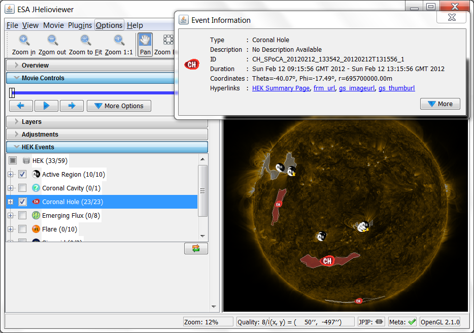
Figure 1: Screenshot from the ESA JHelioviewer tool. The picture on the right displays the AIA 171 image taken on 12 February 2012 at 9:02:12 together with Active Region and Coronal Hole location and chain-code information that are recorded in the HEK. An Event Information window pops up when clicking on an event or feature (here the large Coronal Hole located in the South hemisphere)

In this paper, we present the SPOCA-suite, a set of algorithms that allows separating and extracting CH, AR, and QS on EUV images. We detail the parameterization needed to treat SDO-AIA images. The SPOCA-suite is applied in near real time on AIA archive and produces entries into the AR and CH catalogs of the Heliophysics Event Knowledgebase every four hours. The HEK is further linked through an API to the graphical interface called isolsearch , to the ontology software package of Solarsoft , and to the JHelioviewer visualization tool . The code is written is C++, with some wrapper in IDL and Python. It is available upon request to the corresponding author. Figure 1 shows a screenshot from the ESA JHelioviewer tool with CH and AR boundaries overlays.

This paper is intended as the reference guide for the users of the SPOCA output. It presents the improvements made with respect to the the previous work on the Spatial Possibilistic Clustering Algorithm (Barra et al., 2009). At the core of the SPOCA-suite lies a multi-channel unsupervised fuzzy clustering method that segments EUV images into different regions according to their intensity level.

Development of automated solar feature detection and identification methods has increased dramatically in recent years due to the growing volume of data available. An overview of the fundamental image-processing techniques used in these algorithms is presented in Aschwanden (2010). These techniques are tailored to detect features in various types of observations at different heights in the solar atmosphere, see for example (Martens et al., 2012; Pérez-Suárez et al., 2011). For example, regions of locally intense magnetic flux are observed as dark spots (sunspot) in white light, CaII, or continuum images, as an interlace of positive and negative magnetic field value (magnetic AR) in magnetograms, and as patches of enhanced brightness in chromospheric (plages) and coronal images (AR).

Image segmentation methods are typically classified into three broad categories: region-based methods, edge-based methods and hybrid approaches. Region-based methods seek a partition of the image satisfying an homogeneity criterion (on mono-,multispectral gray levels or higher level attributes such as texture or feature vectors modeling pixels and their neighborhood). The dual edge-based approaches aim at characterising image discontinuities, and thus locating region boundaries. Primal edge-based methods seek for maximum of intensity gradients, using either spatial or frequency filters, or zeros in the Laplacian of the image, often pre processed by a low pass Gaussian filtering, due to the Laplacian sensitivity to noise. Finally, the hybrid methods either consider a cooperation between region and contour approaches, or process some other original method.

Region-based methods for the detection of sunspots include thresholding against background (Pettauer & Brandt, 1997; Colak & Qahwaji, 2008), histogram-based thresholding (Steinegger et al., 1997), region-growing method (Preminger et al., 1997), or bayesian approach (Turmon et al., 2002). (Colak & Qahwaji, 2008; Nguyen et al., 2005) combine thresholding and machine learning techniques to extract and classify sunspots according to the McIntosh system. (Curto et al., 2008; Watson et al., 2009) both use an edge-based approach based on mathematical morphology. Zharkov et al. (2004) employ a hybrid method that combines edge-based and thresholding approaches, whereas Lefebvre & Rozelot (2004) presents a singular spectrum analysis to detect sunspots and faculae at the solar limb.

Active regions as observed by magnetograms can be extracted and characterized by means of region growing techniques (Benkhalil, 2003; McAteer et al., 2005; Higgins et al., 2011), thresholding in the intensity (Qahwaji & Colak, 2006; Colak & Qahwaji, 2009) or wavelet domain (Kestener et al., 2010). Verbeeck et al. (2011) provides a detailed comparaison of outputs from sunspots, magnetic, and coronal active regions using one month of SOHO-EIT data. At the chromospheric level, network and plage regions are separated using thresholding methods (Steinegger et al., 1998; Worden et al., 1999), possibly combined with region-growing techniques (Benkhalil et al., 2006). Coronal active regions are segmented using either local thresholding and region-growing method (Benkhalil et al., 2006), supervised (Dudok de Wit, 2006; Colak & Qahwaji, 2011), or unsupervised (Barra et al., 2009) classification. Revathy et al. (2005) compares segmentation results of pixelwise fractal dimension of EIT images using thresholding, region-growing technique, and supervised classification.

Coronal holes are regions of lower electron density and temperature than the typical quiet Sun, and appear thus as dark regions in EUV and X-ray images. However, automated detection of coronal holes based on intensity thresholding in one wavelength (EIT 28.4nm wavelength in (Abramenko et al., 2009; Obridko et al., 2009) or Soft X-ray images in (Vršnak et al., 2007; Verbanac et al., 2011)) is intrinsically complicated due to the presence of filaments and transient dimmings of same intensity level. To resolve this ambiguity, it is necessary to make use of additional information coming from magnetograms, from other wavelengths, or from time evolution of the feature in order to check the consistency of a CH candidate with actual physical parameters. For example, Henney & Harvey (2005) first use a fixed thresholding based on two-day average He I 1083 nm spectroheliograms and thereafter check the unipolarity of the CH candidates using photospheric magnetograms. de Toma & Arge (2005) use a combination of fixed thresholdings on multiple wavelengths (the four SOHO-EIT bandpasses, He I 1083, magetograms, and H$\alpha$ images) to determine stringent criteria for a region to belong to a CH, whereas  de Toma (2011) use a similar technique on synoptic maps. The approach in (Scholl & Habbal, 2008) is to first perform histogram equalization and fixed thresholding to extract low intensity regions on the four bandpasses of SOHO-EIT. In a second stage statistics on magnetic field parameters measured by SOHO-MDI are evaluated to discriminate between filaments and coronal holes. A similar methodology is used in Krista & Gallagher (2009) with the difference that it first detects low intensity regions using local histogram of SOHO-EIT, STEREO-EUVI, and Hinode-XRT images. Other methods include a watershed approach (Nieniewski, 2002), perimeter tracing for polar coronal hole using morphological transform and thresholding (Kirk et al., 2009), and the use of imaging spectroscopy to separate quiet sun from coronal hole emission (Malanushenko & Jones, 2005). Finally, the classification approach in (Dudok de Wit, 2006; Colak & Qahwaji, 2011; Barra et al., 2009) allows separating both active regions and coronal holes using brightness intensity observed in one or in multiple bandpasses.

In this paper, we describe the improvements made with respect to the paper in (Barra et al., 2009) in terms of robustness and stability. For example, the segmentation in Barra et al. (2009) required the pre-determination of centers of classes before applying it on a large data set, which is difficult to implement when the segmentation is performed continuously on a stream of data.

As part of the Feature Finding Team (Martens et al., 2011), programs have been specifically written to run in near real time on SDO-AIA images. It results in two separate modules: SPOCA-AR module for Active Regions, and SPOCA-CH for coronal.

Section 2 below describes the algorithm, and Section 3 provides some illustration of the algorithm on SDO-AIA data.

2 The SPOCA-suite

The SPOCA-suite implements three types of fuzzy clustering algorithms: the Fuzzy C-means (FCM), a regularized version of FCM called Possiblistic C-means (PCM) algorithm, and a Spatial Possiblistic Clustering Algorithm (SPOCA) that integrates neighboring intensity values.

The description of the segmentation process in terms of fuzzy logic was motivated by the facts that information provided by an EUV solar image is noisy and subject to both observational biases (line-of-sight integration of a transparent volume) and interpretation (the apparent boundary between regions is a matter of convention). Fuzzy measures are able to represent ill-defined classes (without a clear-cut boundary) in a natural way.

Let $x_{j}\in\mathbb{R}^{p}$ be a $p$-dimensional feature vector that describes the Sun at a particular location. In our case, $x_{j}$ is a $N-$dimensional vector of intensities recorded in $p$ different channels. A fuzzy clustering algorithm searches for $C$ compact clusters amongst the $x_{j}$’s in $X=\{x_{j}\}$. It does so by computing both a fuzzy partition matrix $U=(u_{ij}),1\leq i\leq C,1\leq j\leq N$ and the cluster centers $B=(b_{i}\in\mathbb{R}^{p},1\leq i\leq C)$. The scalar $u_{i,j}=u_{i}({x_{j}})\in[0,1]$ is called the membership degree of ${x_{j}}$ to class $i$.

We now describe the FCM and PCM algorithm as they are used in the SPOCA-suite. A description of the Spatial Possibilistic clustering algorithm is available in Barra et al. (2009).

2.1 Fuzzy Clustering Algorithm

Since its introduction by Bezdek (Bezdek, 1981), the Fuzzy C-Means (FCM) algorithm was widely used in pattern recognition and image segmentation, in various fields including medical imaging (Philipps et al., 1995; Bezdek et al., 1997), remote sensing images (Rangsanseri & Thitimajshima, 1998; Melgani et al., 2000), color image segmentation in vision (Baker et al., 2003). As compared to the crisp (traditional) method, the fuzzy segmentation more often reaches a global optimal, rather than merely a local optimum (Trauwaert et al., 1991).

The idea behind FCM is the minimisation of the total intracluster variance:

$$J_{FCM}(B,U,X)=\displaystyle\sum_{i=1}^{C}\displaystyle\sum_{j=1}^{N}u_{ij}^{m}d^{2}({x_{j}},{b_{i}})$$ (1)

subject to

$$(\forall i\in\{1\cdots C\})\displaystyle\sum_{j=1}^{N}u_{ij}<N\quad\textrm{ and }\quad(\forall j\in\{1\cdots N\})\displaystyle\sum_{i=1}^{C}u_{ij}=1$$ (2)

where $d$ is a metric in $\mathbb{R}^{p}$ (typically, the Euclidian distance), and $m$ is a parameter that controls the degree of fuzzification ($m=1$ means no fuzziness). In practice, a value of $m=2$ is often chosen, as it allows for a fast computation in the iterative scheme. In our application we consider either one ($p=1$) or two channels ($p=2$).

The minimization of (1) is reached when

$$u_{ij}=\frac{1}{\sum_{k=1}^{C}\left(\frac{d^{2}(x_{j},b_{i})}{d^{2}(x_{j},b_{k})}\right)^{1/(m-1)}}\quad\textrm{ and }\quad b_{i}=\frac{\sum_{k=1}^{N}u_{ik}^{m}x_{k}}{\sum_{k=1}^{N}u_{ik}^{m}}$$ (3)

The values satisfying (3) are obtained through an iterative procedure.

The shortcomings of FCM are of two types. First, it is sensitive to noise and outliers (Krishnapuram & Keller, 1993). Second, it is theoretically not satisfying since the value of one center in (3) depends on the value of the other centers.

In practice however FCM provides the best results for extracting Coronal Holes out of the (almost noise free) 19.3nm AIA images. Given the size of AIA images, FCM is applied on the histogram of normalized intensity values, rather than on individual values. The normalization consists in dividing by exposure time, correcting for limb brightness enhancement, and dividing by the median value (see Section 2.5). A binsize of 0.01 for the histogram provides the same numerical precision as if individual values were used.

2.2 Possibilistic C-means algorithm

To obtain a formulation for $u_{ij}$ that depends only on the distance to the center of class $i$, Krishnapuram & Keller (1993, 1996) propose to minimize the objective function

$$J_{PCM}(B,U,X)=\sum_{i=1}^{C}\left(\sum_{j=1}^{N}u_{ij}^{m}d^{2}({x_{j}},{b_{i}})+\eta_{i}\sum_{j=1}^{N}(1-u_{ij})^{m}\right)$$ (4)

subject to

$$(\forall i\in\{1\cdots C\})\displaystyle\sum_{j=1}^{N}u_{ij}<N\quad\mbox{and}\quad(\forall j\in\{1\cdots N\})\displaystyle\max_{i}u_{ij}>0$$ (5)

The first term of $J_{PCM}$ in (4) is the intracluster variance, whereas the second term, stemming from the relaxation of the probabilistic constraint in (2), enforces $u_{ij}$ to depend only on $d({x_{j}},{b_{i}})$.

Parameter $\eta_{i}$ in (4) is homogeneous to a squared distance. It can be fixed, or updated at each iterations. Krishnapuram & Keller (1993) proposed to compute $\eta_{i}$ as the intra-class dispersion:

$$\eta_{i}=\frac{\displaystyle\sum_{j=1}^{N}u_{ij}^{m}d^{2}({x_{j}},{b_{i}})}{\displaystyle\sum_{j=1}^{N}u_{ij}^{m}}$$ (6)

The solution of the minimization of (4) satisfies:

$$u_{ij} = \left[1+\left(d^{2}({x_{j}},{b_{i}})/\eta_{i}\right)^{\frac{1}{m-1}}\right]^{-1}$$ (7)

$$b_{i} = \displaystyle\sum_{j=1}^{N}u_{ij}^{m}{x_{j}}/\displaystyle\sum_{j=1}^{N}u_{ij}^{m}$$ (8)

In practice, PCM is initialized by one iteration of FCM, which allows for computation of $\eta_{i}$ as in (6). Krishnapuram & Keller (1993) proved the convergence of iteration (7)-(8) for fixed $\eta$. PCM is more robust to noise and outliers than FCM, and provides independent functions $\mathbf{u_{i}}=\{u_{ij},j=1,\ldots,N\}$. It must be corrected however from coincident clustering (Section 2.2.1), and a proper choice of the parameter $\eta$ must be made (Section 2.2.2). The SPOCA-AR module of the HEK uses this corrected PCM algorithm on the AIA 17.1nm and 19.3nm bandpasses. Similar to the SPOCA-CH module, it is applied on histogram intensity values rather than on individual pixel intensity values.

2.2.1 Coincident Clustering

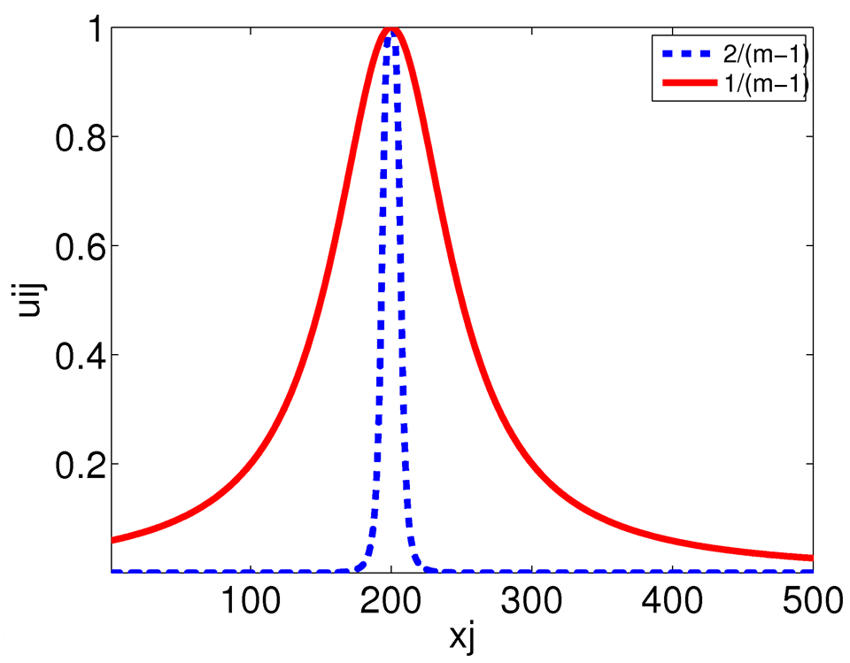
Figure 2: Comparaison of membership functions $u_{ij}$ when the exponent is chosen equal to $1/(m-1)$ (red line) and $2/(m-1)$ (blue dashed line). The blue dashed line is more compact, which will lead to the choice of distinct centres of classes.

The original PCM suffers from convergence to a unique center. This is a typical feature of possibilistic clustering algorithms called ‘coincident clustering’ (Krishnapuram & Keller, 1996). To circumvent this problem we use membership functions $u_{ij}$ which are more compact and hence do not overlap so easily. More precisely, exponent $1/(m-1)$ in (7) is replaced by $2/(m-1)$, see Figure 2 for a graphical representation. We call PCM2 the algorithm where the exponent in the membership function $u_{ij}$ is taken equal to $2/(m-1)$.

2.2.2 Constraints on the parameter $\eta_{i}$

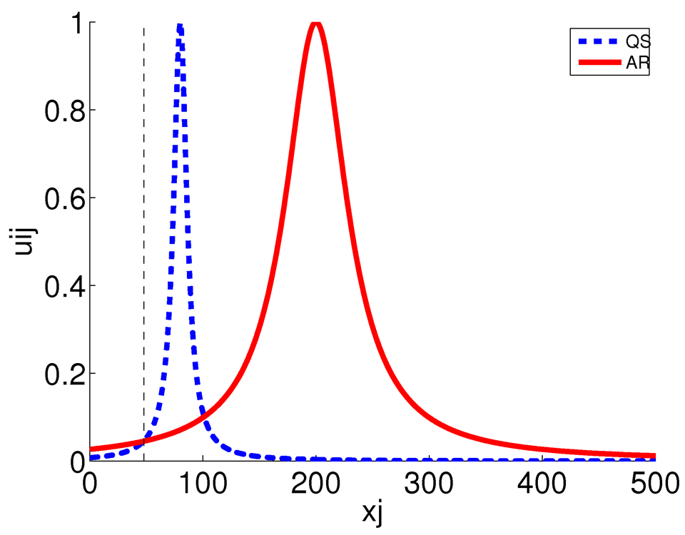
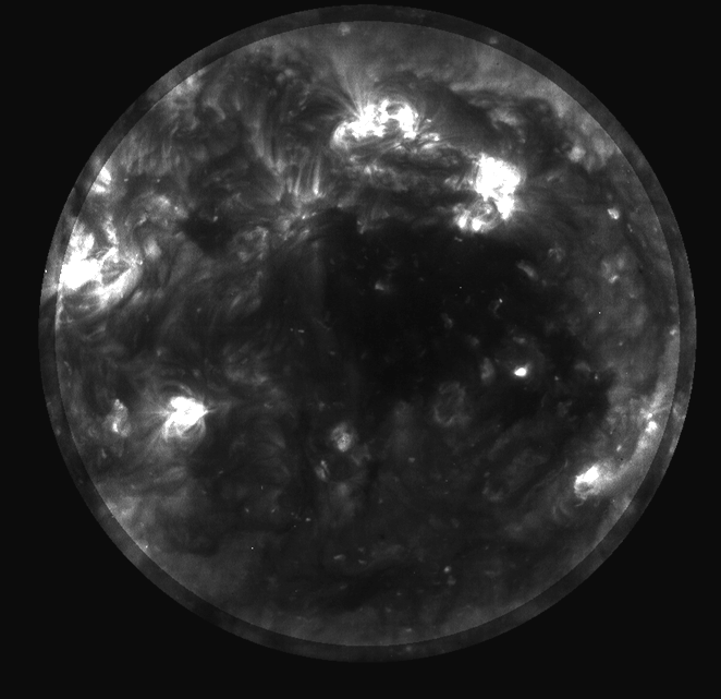
(a) membership function for AR and QS	(b) EIT 195 $\AA$ image
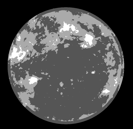
(c) Original segmented map	(d) Segmented map with constraints

Figure 3: (a) Illustration of membership functions $u_{ij}$ for QS and AR descriptors $x_{j}$. Because of the larger spread in intensity values of the AR, small values of $x_{j}$ may have a larger AR membership than QS membership. (b) EIT 195 $\AA$ from January 1, 2000 with correction of limb brightness (c) Segmentation using original PCM algorithm: darkest part are classified as Active regions (d) Segmentation using PCM with constraints on $\eta$-values

The dynamical range of intensities differs amongst the CH, QS, and AR classes, with active regions having the largest spread in intensities. The parameter $\eta_{i}$ as computed in (6) can be viewed as a measure of dispersion or variance within a class. In case $\eta_{AR}$ becomes prohibitively large, the value of $u_{AR,j}$ for dark pixels $x_{j}$ can be higher than $u_{QS,j}$ or $u_{CH,j}$, as illustrated in Figure 3(a). To avoid this situation we must enforce the following inequalities, as derived in Appendix A:

$$\frac{\eta_{QS}}{\eta_{CH}}<\frac{b_{QS,q}}{b_{CH,q}},\frac{\eta_{AR}}{\eta_{CH}}<\frac{b_{AR,q}}{b_{CH,q}},\frac{\eta_{AR}}{\eta_{QS}}<\frac{b_{AR,q}}{b_{QS,q}},\mbox{ for }q=1,\dots,p.$$ (9)

with $b_{CH,q},b_{QS,q},$ and $b_{AR,q}$ the center of classes for the q-th channel and for CH, QS and AR respectively. Figure 3 shows an example of segmentation with and without constraints on $\eta_{i}$. Without constraints, some CH areas gets classified in the same class as the AR. This problem is solved when constraints (9) are introduced.

For solar EUV images, the combination of the iteration scheme (6)-(8) tends to produce $\eta_{CH}$-values that converge to zero. Due to the condition (9) on $\eta_{QS}$ and $\eta_{AR}$, these two parameters are dragged along to converge to zero as well. Our iterative scheme therefore freezes the value of $\eta_{i}$ when it has changed by a factor $\alpha$ with respect to its starting value. In other words, formula (6) is used until iteration ${it}$ is reached with:

$$\eta_{i}^{it}/\eta_{i}^{1}>\alpha{\rm\ or\ }\eta_{i}^{1}/\eta_{i}^{it}>\alpha~{}.$$

For the next iterations, we keep $\eta_{i}^{it}$ fixed. Satisfactory results have been obtained on a variety of datasets and instruments with $\alpha=100$.

2.3 Smooth variation of center values

In order to have a smooth variation of the center values over time, the centers chosen at time $t$ in the HEK are in fact the median of the last 10 centers obtained at previous time stamp $t,t-1,\ldots,t-9$. In order to get the membership map corresponding to this smooth value of the center $b_{i}$ an attribution procedure using left part of formula (3) (for FCM), or formula (7)(for PCM) is performed.

2.4 Segmented maps

Given the membership maps $U$ and centers $B$ a segmention map can be obtained using various decision rules

Maximum:

The most common rule is to attribute a pixel $j$ to the class $c$ for which it has the maximum membership value: $\{u_{c,j}=\max_{i\in\{{1,\ldots,C}\}}u_{ij}\}$. This rule is used in the SPOCA-CH module.

Threshold

On EUV images the QS class contains typically the largest number of pixels, and hence the center of QS class is the most stable over time. On the contrary, the cardinality of points belonging to the AR class varies a lot over time, resulting in a high variation of center of AR class. In order to have a stable segmentation of AR over time, the SPOCA-AR module therefore uses a threshold on the QS membership class to define the belonginess of a pixel to the AR class. All pixels $j$ which are higher than $b_{QS}$ and for which $u_{QS,i}$ is lower than 0.0001 are attributed to the AR class.

Closest

This rule attributes a pixel to the class for which the Euclidian distance to the center class is the smallest.

Merge

This more complex procedure uses sur-segmentation and merging of classes and has been described in (Barra et al., 2009).

2.5 Pre-processing

Some pre-processing steps are needed in order to obtain an accurate segmentation of the images.

First, images are calibrated using solar software routines and intensities are divided by the exposure time.

Second, the SPOCA-suite might be applied on linear or on square root transformed images. A square root transform is akin to an Anscombe transform (Anscombe, 1948) which has the property of approximately converting Poisson noise into Gaussian noise. This is especially useful for the extraction of low-intensity regions such as coronal holes which are affected by Poisson noise.

Third, the limb brightening effect has to be corrected before any segmentation based on intensity can be applied. A first correction was proposed in (Barra et al., 2009). It consists of applying a a polar transform to represent the image $I$ in a $(\rho,\theta)$ plane, with origin at the solar disc center. The polar transform is a conformal mapping from points in the cartesian plane $(x,y)$ to points in this polar plane, described by: $\rho=\sqrt{x^{2}+y^{2}},\theta=atan(y/x)$. The intensity is specified as a function of $\rho$ using the integral $g(\rho)=\int_{0}^{2\pi}I(\rho,\theta)d\theta$. Denoting $m_{\odot}$ the median value of intensities on the on-disc part of the Sun, the image $I_{corr}$ corrected for the enhanced brightness at the limb is computed as:

$$I_{corr}(\rho,\theta)=m_{\odot}\frac{I(\rho,\theta)}{g(\rho)}~{},$$ (10)

for values of $\rho$ ranging between 95% and 105% $R_{\odot}$. $I_{corr}$ is then finally remapped to the cartesian plane.

Such abrupt correction leads to disconintuities in the images around these radial distances, as can be seen on the images in Figure 3. We propose instead to apply a correction $I_{smooth}$:

$$I_{smooth}(x,y)=\left(1-f(\rho(x,y))\right)I(x,y)+f(\rho(x,y))I_{corr}(x,y).$$ (11)

where $f(\rho(x,y))$ introduces a smooth transition between the zones not corrected (when $\rho$ is between 0 and $r_{1}$ or above $r_{4}$) and the zones $\rho\in[r_{2},r3]$ that are fully corrected using equation (10):

$$f(\rho)=\left\{\begin{array}[]{lll}0&\mbox{if}&\rho\leq r_{1}{\rm\ or\ }\rho\geq r_{4}\\ 1&\mbox{if}&\rho\in[r_{2},r_{3}]\\ \frac{1}{2}\sin\Big{(}\frac{\pi}{r_{2}-r_{1}}(\rho-\frac{r_{1}+r_{2}}{2})\Big{)}+\frac{1}{2}&\mbox{if}&r_{1}\leq\rho\leq r_{2}\\ \frac{1}{2}\sin\Big{(}\frac{\pi}{r_{4}-r_{3}}(\rho+\frac{r_{4}-3r_{3}}{2})\Big{)}+\frac{1}{2}&\mbox{if}&r_{3}\leq\rho\leq r_{4}\end{array}\right.$$

A simulation study was conducted to determine the optimal values of $[r_{1},r_{2},r_{3},r_{4}]$ for a given instrument. The mean square error (MSE) between corrected limb values and the on-disc median intensity is used as criterion. For SDO-AIA, the values that minimizes the MSE are (in % of $R_{\odot}$) are $[70,95,108,112]$ . Fnally, $I_{smooth}$ is divided by its median value.

2.6 Region extraction and post-processing

To extract regions (that will be labelled as Active Regions or as Coronal Holes) from segmented maps, the following post-processing steps are implemented:

1. Compute a sinusoidal projection map (Snyder, 1987). This improves the determination of regions towards the limb.

2. Clean the segmented map by removing elements smaller than 6 arcsec using a morphological erosion

3. Aggregate neighboring blobs by performing a morphological closing, which consists of a dilatation by 32 arcsec followed by an erosion.

4. Compute the inverse of sinusoidal projection

The reader is refered to Barra et al. (2009) for an introduction to mathematical morphology in this context. The equirectangular and Lambert cylindrical projections are also implemented in the SPOCA-suite. Our test on SDO data shows that the sinusoidal projection gives the best results.

To remove spurious regions, a final cleaning is performed as follows. Active regions smaller than $1500~{}\mbox{arcsec}^{2}$ and coronal holes smaller than $3000\mbox{arcsec}^{2}$ are discarded.

Moment statistics and properties such as area, barycenter location, bounding box are then computed.

A coronal hole has relatively smooth boundaries. Having an accurate estimation of its shape and localisation is crucial for space weather purpose, since coronal holes are most geoeffective when they are located at the central meridian and near the equator. We computed a chain code for the coronal holes using per default a maximum of 100 points to describe the contour. The details of the algorithm are described in Appendix B. Similarly, we provided a chain-code for Active Regions. Note however that in order to represent in an optimal way the non-smooth AR boundaries more than 100 points would be needed.

2.7 Tracking over time

Following the aggregation of regions described in the previous section, an active region is defined as a coherent group of corresponding active region blobs, and similarly for the coronal holes. The goal of tracking is to appoint the same ID number to a physical region (AR or CH) over time. A region observed at timestamp $t$ can follow the region observed at previous timestamp, but it can also split (and produce two children), or it can merge with other neighboring regions.

Our tracking scheme amounts to create a directed graph $(N,E)$ where $N$ is the list of nodes representing individual regions and $E$ is the list of edges between regions. An edge between a region observed at time $t_{1}$ and another observed at time $t_{2}$ is created if their time difference $t_{2}-t_{1}$ is smaller than some value, if they overlay, and if there is not already a path between them. It is possible to first derotate the regions maps before comparing them. This is necessary when large time difference are involved.

Coronal holes are long-lived features. We can include this information in the tracking and keep only coronal holes that are older than three days. Our analysis of SDO images during the year 2011 shows that a coronal hole candidate detected for more than three consecutive days exhibits the expected magnetic properties characteristics of unipolar regions. Hence we report to the HEK only the CHs that are older than three days.

3 Analysis of SDO-AIA images

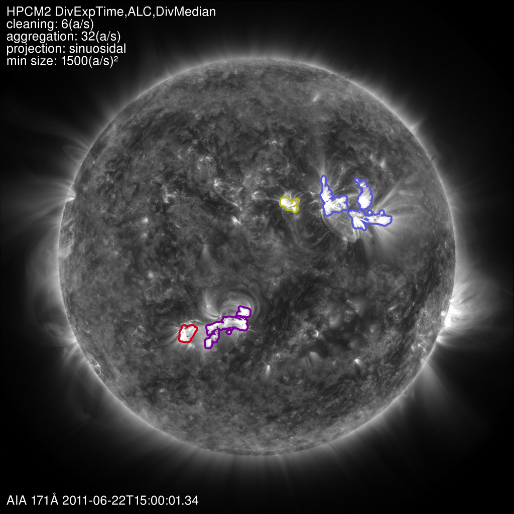
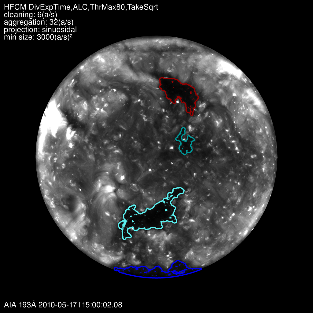
(a) Overlay of AR map on AIA 171 $\AA$	(b) Overlay of CH map on AIA 193 $\AA$

Figure 4: (a) Overlay of a AR map created using AIA 171 and 193 $\AA$ onto the corresponding AIA 171$\AA$ image taken on 20110622 at 15:00 (b) Overlay of CH map created using AIA 193 $\AA$ onto the corresponding AIA 193 $\AA$ image taken on 20100517 at 15:00

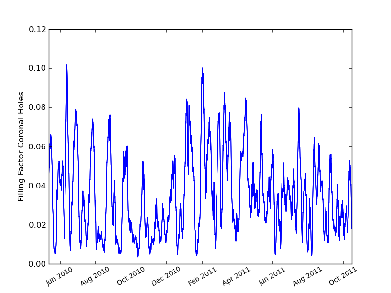
Figure 5: Coronal Holes Filling factor extracted from SPOCA results, from 1st June 2010 till 31 October 2011.

We now illustrate the results from SPoCA using SDO images. Figure 4 shows an example of overlays of AR and CH maps onto the corresponding AIA images. Figure 5 shows an example of statistics given by the SPOCA algorithm. for the period June 2010 till October 2011.

4 Conclusion

We describe here the algorithm implemented int eh SPOCA-AR and SPOCA-CH modules of the HEK. This provides catalogs or Active Regions and Coronal Holes containing properties such as localisation (through a bounding box or a chain code), area, moments of intensities. Contours can also be visualized through isolsearch interface or within the JHelioviewer visualization software.

These catalogs have many different applications, one of them being the determination of filling factors for CH, AR, QS, to be included into (semi-)empirical models of irradiance.

In future reseach, we plan on improving criteria for distinguishing between filaments and coronal holes. At present the distinction is based on area (we retain only CH larger than $3000$ arcsec²) and duration (we retain only CH older than 3 days), as our study on the year 2010-2011 shows this extract CH candidates having appropriate magnetic properties. As we reach solar maxima however, such distinction between filaments channel and coronal holes might become more problematic.

Appendix A Constraints on regularization parameter

All algorithms based on Possibilistic C-means strongly depends on the choice of the regularization parameter $\eta$. Various more or less elaborated procedures have been proposed in the literature, see for example Krishnapuram & Keller (1996). An intuitive choice is to compute $\eta_{i}$ as the intra-class dispersion, as in equation (6). Problems arise however when the underlying classes have a widely different intra-class variance. For example, the highly variable AR class on EUV images may include in the final segmentation the darkest part of what should be the Coronal Hole class.

To understand this phenomena, consider two classes $C_{1}$ and $C_{2}$ with centers $b_{1}$ and $b_{2}$. , Suppose $b_{1p}<b_{2p},\forall p=1,\dots,P$, where $P$ is the dimension of the feature space. We show that under certain circumstances, $u_{2j}$ can exceed $u_{1j}$ for values of $x_{j}$ where $x_{jp}<b_{1p},\forall p=1,\dots,P$.

Let us first determine the locus of points $x_{j}$ where $u_{1j}=u_{2j}$. By equation (7) we found that $u_{1j}=u_{2j}$ if and only if

$$\frac{d^{2}(x_{j},b_{1})}{\eta_{1}}=\frac{d^{2}(x_{j},b_{2})}{\eta_{2}}.$$ (12)

If $\eta_{1}=\eta_{2}$, the solution is a hyperplane through the middle of $b_{1}$ and $b_{2}$, and there are no undesired effects. In case $\eta_{1}\neq\eta_{2}$, and for the Euclidean distance, the above is equivalent to saying that $x_{j}$ lies on a circle with center

$$c=\frac{\eta_{2}b_{1}-\eta_{1}b_{2}}{\eta_{2}-\eta_{1}}$$ (13)

and radius

$$r=\frac{\sqrt{\eta_{1}\eta_{2}}}{|\eta_{2}-\eta_{1}|}\cdot d(b_{1},b_{2}).$$ (14)

We consider only the case $\eta_{1}<\eta_{2}$, as this is the case for the classes CH, QS and AR as they arise in EUV images. In this case, $c$ will lie relatively close to $b_{1}$, at the “opposite side” from $b_{2}$. All points $x_{j}$ inside the circle will satisfy $u_{1j}>u_{2j}$, and hence belong to class 1. All points $x_{j}$ outside the circle will satisfy $u_{2j}>u_{1j}$, and hence will be classified as belonging to class 2. This is unwanted behavior for those points for which some $x_{jp}<b_{1p}$. In order to avoid this situation, we can select $\eta$-values in such a way that the circle center $c$ lies below all coordinate axes. The result is that for all points $x_{j}$ in the circle, all positive points “below” it are also in the circle. Hence whenever a point $x_{j}$ belongs to class 1, all points “below” $x_{j}$ also belong to class 1. So we want $c_{p}<0,\forall p=1,\dots,{\rm dim}$, which is equivalent to the following conditions on $\eta_{1}$ and $\eta_{2}$:

$$\frac{\eta_{2}}{\eta_{1}}<\frac{b_{2p}}{b_{1p}},\forall p=1,\dots,{\rm dim}$$ (15)

Appendix B Computation of chain code

Chain coding aims at representing the boundary of an object in digitized images. It is based on the idea of following the outer edge of the object and storing the direction when travelling along the boundary (Freeman, 1961). In the SPOCA-suite, we use a representation of the chain code with eight directions, as is commonly done in the literature. Such represenation is however of the same length as the perimeter of the object under consideration, which in many cases is too long. In a second step, we thus find a polygonal approximation to the perimeter that has a maximal number of edges, and for which the distance from any point in the perimeter to the polygon does not exceed a given accuracy.

The algorithm proceeds as a recursive refinement. The main axis of the contour is first extracted, providing the first two vertices. Each polygon edge is then recursively split by introducing a new vertex at the most distant associated contour point, until the desired accuracy is reached. More precisely, the algorithm runs as follows:

1. Initialize the polygon with points $p_{1}$ and $p_{2}$ of the perimeter that are furthest away from each other.

2. Let $i=3$

3. For each segment in the polygon find the point on the perimeter that have the furthest distance to the polygonal line-segment. If this distance is larger than a threshold mark the point with a label $p_{i}$

4. Renumber the points so that they are consecutive

5. Increase $i$

6. If no points have been added then finish, otherwise go back to step 3.

Within the HEK, a maximal number of 100 points is considered to be sufficient for a reasonable approximation of CH boundaries.

References

- (1)
- Abramenko et al. (2009) Abramenko, V., Yurchyshyn, V., & Watanabe, H. 2009, Sol. Phys., 260, 43
- Anscombe (1948) Anscombe, F. J. 1948, Biometrika, 35, 246
- Aschwanden (2010) Aschwanden, M. J. 2010, Sol. Phys., 262, 235
- Baker et al. (2003) Baker, J., Campbell, D., & Bodnarova, A. 2003, in Proceedings of ASC’2003 - Artificial Intelligence and Soft Computing, 385–389
- Barra et al. (2009) Barra, V., Delouille, V., Kretzschmar, M., & Hochedez, J.-F. 2009, A&A, 505, 361
- Benkhalil et al. (2006) Benkhalil, A., Zharkova, V. V., Zharkov, S., & Ipson, S. 2006, Sol. Phys., 235, 87
- Benkhalil (2003) Benkhalil, A. et al.. 2003, in Proceedings of the AISB’03 Symposium on Biologically-inspired Machine Vision, Theory and Application, University of Wales, Aberystwyth, 7th - 11th April 2003, ISBN 1-902956-33-1, 66–73
- Bezdek (1981) Bezdek, J. 1981, Pattern recognition with fuzzy objective function algorithms (New-York: Plenum Press,)
- Bezdek et al. (1997) Bezdek, J., L.O.Hall, Clark, M., Goldof, D., & Clarke, L. 1997, Stat Methods Med Res, 6, 191
- Colak & Qahwaji (2008) Colak, T. & Qahwaji, R. 2008, Sol. Phys., 248, 277
- Colak & Qahwaji (2009) Colak, T. & Qahwaji, R. 2009, Space Weather, 7, 6001
- Colak & Qahwaji (2011) Colak, T. & Qahwaji, R. 2011, Sol. Phys., 388
- Curto et al. (2008) Curto, J. J., Blanca, M., & Martínez, E. 2008, Sol. Phys., 250, 411
- de Toma (2011) de Toma, G. 2011, Sol. Phys., 274, 195
- de Toma & Arge (2005) de Toma, G. & Arge, C. N. 2005, in Astronomical Society of the Pacific Conference Series, Vol. 346, Large-scale Structures and their Role in Solar Activity, ed. K. Sankarasubramanian, M. Penn, & A. Pevtsov, 251
- Dudok de Wit (2006) Dudok de Wit, T. 2006, Solar Physics, 239, 519
- Freeman (1961) Freeman, H. 1961, Proceedings of IRE Translation Electron Computer, 260, new York
- Henney & Harvey (2005) Henney, C. J. & Harvey, J. W. 2005, in Astronomical Society of the Pacific Conference Series, Vol. 346, Large-scale Structures and their Role in Solar Activity, ed. K. Sankarasubramanian, M. Penn, & A. Pevtsov, 261
- Higgins et al. (2011) Higgins, P. A., Gallagher, P. T., McAteer, R. T. J., & Bloomfield, D. S. 2011, Advanced Space Research, 47, 2105
- Kestener et al. (2010) Kestener, P., Conlon, P. A., Khalil, A., et al. 2010, ApJ, 717, 995
- Kirk et al. (2009) Kirk, M. S., Pesnell, W. D., Young, C. A., & Hess Webber, S. A. 2009, Sol. Phys., 257, 99
- Krieger et al. (1973) Krieger, A. S., Timothy, A. F., & Roelof, E. C. 1973, Sol. Phys., 29, 505
- Krishnapuram & Keller (1993) Krishnapuram, R. & Keller, J. 1993, IEEE Transactions on Fuzzy Systems, 1, 98
- Krishnapuram & Keller (1996) Krishnapuram, R. & Keller, J. 1996, IEEE Transactions on Fuzzy Systems, 4, 385
- Krista & Gallagher (2009) Krista, L. D. & Gallagher, P. T. 2009, Sol. Phys., 256, 87
- Lefebvre & Rozelot (2004) Lefebvre, S. & Rozelot, J. 2004, Sol. Phys., 219, 25
- Malanushenko & Jones (2005) Malanushenko, O. V. & Jones, H. P. 2005, Sol. Phys., 226, 3
- Martens et al. (2011) Martens, P. C. H., Attrill, G. D. R., Davey, A. R., et al. 2011, Sol. Phys.
- Martens et al. (2012) Martens, P. C. H., Attrill, G. D. R., Davey, A. R., et al. 2012, Sol. Phys., 275, 79
- McAteer et al. (2005) McAteer, R. T. J., Gallagher, P. T., Ireland, J., & Young, C. A. 2005, Sol. Phys., 228, 55
- Melgani et al. (2000) Melgani, F., Hashemy, B. A., & Taha, S. 2000, IEEE Transaction on Geoscience and Remote Sensing, 38, 287
- Nguyen et al. (2005) Nguyen, S. H., Nguyen, T. T., & Nguyen, H. S. 2005, in Lecture Notes in Computer Science, Vol. 3642, Rough Sets, Fuzzy Sets, Data Mining, and Granular Computing, ed. D. Slezak, J. Yao, J. F. Peters, W. Ziarko, & X. Hu (Berlin / Heidelberg: Springer Berlin / Heidelberg), 263–272
- Nieniewski (2002) Nieniewski, M. 2002, in Proceedings of the SOHO 11 Symposium on From Solar Min to Max: Half a Solar Cycle with SOHO, ed. N. E. P. D. A. Wilson. Noordwijk, 323–326
- Obridko et al. (2009) Obridko, V. N., Shelting, B. D., Livshits, I. M., & Asgarov, A. B. 2009, Sol. Phys., 260, 191
- Pérez-Suárez et al. (2011) Pérez-Suárez, D., Higgins, P. A., McAteer, R. T. J., Bloomfield, D. S., & Gallagher, P. T. 2011, in Applied Signal and Image Processing: Multidisciplinary Advancements, ed. R. Qahwaji, R. Green, & E. Hines (Hershey, Pennsylvania: IGI Global), 207–225
- Pettauer & Brandt (1997) Pettauer, T. & Brandt, P. 1997, Solar Physics, 175, 197
- Philipps et al. (1995) Philipps, W., Velthuizen, R., & S.Phuphanich. 1995, Magn Reson Imaging, 13, 277
- Preminger et al. (1997) Preminger, D., Walton, S., & Chapman, G. 1997, Solar Physics, 171, 303
- Qahwaji & Colak (2006) Qahwaji, R. & Colak, T. 2006, I. J. Comput. Appl., 13, 9
- Rangsanseri & Thitimajshima (1998) Rangsanseri, Y. & Thitimajshima, P. 1998, in Proceedings of IGARSS, Vol. 5, 2507–2509
- Revathy et al. (2005) Revathy, K., Lekshmi, S., & Nayar, S. R. P. 2005, Sol. Phys., 228, 43
- Scholl & Habbal (2008) Scholl, I. F. & Habbal, S. R. 2008, Sol. Phys., 248, 425
- Snyder (1987) Snyder, J. P. 1987, Map Projections: A Working Manual, USGS Numbered Series No. 1365 (Geological Survey (U.S.))
- Steinegger et al. (1997) Steinegger, M., Bonet, J., & Vazquez, M. 1997, Solar Physics, 171, 303
- Steinegger et al. (1998) Steinegger, M., Bonet, J., Vazquez, M., & Jimenez, A. 1998, Solar Physics, 177, 279
- Trauwaert et al. (1991) Trauwaert, E., Kaufman, L., & Rousseeuw, P. 1991, Fuzzy Sets and Systems, 42, 213
- Turmon et al. (2002) Turmon, M., Pap, J. M., & Mukhtar, S. 2002, ApJ, 568, 396
- Verbanac et al. (2011) Verbanac, G., Vršnak, B., Veronig, A., & Temmer, M. 2011, A&A, 526, A20
- Verbeeck et al. (2011) Verbeeck, C., Higgins, P. A., Colak, T., et al. 2011, Sol. Phys., 369
- Vršnak et al. (2007) Vršnak, B., Temmer, M., & Veronig, A. M. 2007, Sol. Phys., 240, 315
- Watson et al. (2009) Watson, F., Fletcher, L., Dalla, S., & Marshall, S. 2009, Sol. Phys., 260, 5
- Worden et al. (1999) Worden, J., Woods, T., Neupert, W., & Delaboudiniere, J. 1999, The Astrophysical Journa, 965
- Zharkov et al. (2004) Zharkov, S., Zharkova, V., Ipson, S., & Benkhalil, A. 2004, in Lecture Notes in Computer Science, Vol. 3215, Knowledge-Based Intelligent Information and Engineering Systems (Berlin / Heidelberg: Springer Berlin / Heidelberg), 446–452