A cosmological solution of Regge calculus

Abstract

We revisit the Regge calculus model of the Kasner cosmology first considered by S. Lewis. One of the most highly symmetric applications of lattice gravity in the literature, Lewis’ discrete model closely matched the degrees of freedom of the Kasner cosmology. As such, it was surprising that Lewis was unable to obtain the full set of Kasner-Einstein equations in the continuum limit. Indeed, an averaging procedure was required to ensure that the lattice equations were even consistent with the exact solution in this limit. We correct Lewis’ calculations and show that the resulting Regge model converges quickly to the full set of Kasner-Einstein equations in the limit of very fine discretization. Numerical solutions to the discrete and continuous-time lattice equations are also considered.

1 Introduction

The discrete formulation of gravity proposed by T. Regge in 1961 [1] has been deployed in a wide variety of settings, from probing the foundations of gravity and the quantum realm [2, 3] to numerical studies of classical gravitating systems [2, 4]. Regge calculus continues to be used in new and diverse ways; recent examples include Ricci flow [5] and as an explanation of dark energy [6].

In this paper we re-examine the Regge calculus model of the vacuum Kasner cosmology first considered by Lewis [7], with the goal of gaining insight into the continuum limit of this discrete approach to gravity. In a general setting the structural differences between a continuous manifold and a discrete simplicial lattice lead to difficulties in directly comparing the Regge and Einstein equations or their solutions, with a single Regge equation per edge in the lattice compared with ten Einstein equations per event in spacetime. We expect many more simplicial equations than Einstein equations in a general simulation, and some form of averaging must be expected before the equations (or their solutions) can be compared.

Lewis [7] studied both the Kasner and spatially flat Friedmann-Lemaître-Robertson-Walker (FLRW) cosmologies using a regular hypercubic lattice. We only consider the Kasner solution in this paper, where the high degree of symmetry, without the added complication of matter, allows explicit examination of the Regge equations in the continuum limit. By aligning the degrees of freedom of the lattice with the continuum metric components, Lewis was able to avoid the issue of averaging and make direct comparisons between the Regge equations and the Kasner-Einstein equations in the continuum limit. Unfortunately, Lewis was only able to recover one of the four Einstein equations in this limit, and even this was only possible after the equations were carefully averaged [7]. Without this averaging it is not clear that the equations obtained by Lewis actually represent the Kasner cosmology.

We show that Lewis neglected a vital portion of the simplicial curvature arising from the two-dimensional spacelike lattice faces that lie on constant time hypersurfaces. The Kasner cosmology has zero intrinsic curvature on constant time hypersurfaces, so the lattice curvature concentrated on spacelike faces – measured on a plane with signature “-+” orthogonal to the face – make an important contribution to the total lattice curvature. We show that when these curvature terms are included, the discrete equations exactly reproduce the Kasner-Einstein equations in the limit of very fine triangulations without the need to average.

In addition to reconsidering Lewis’ analytic work on the spatially flat, anisotropic Kasner cosmology [7], we construct numerical solutions to the discrete and continuous-time lattice equations. This builds on the previous work of Collins and Williams [8] and Brewin [9] on highly symmetric, continuous time, closed FLRW cosmologies, and the (3+1)-dimensional numerical study of the Kasner cosmology by Gentle [10] with discrete time and coarse spatial resolution. We begin by briefly describing the continuum Kasner solution.

2 The Kasner cosmology

The Kasner solution [11] is a vacuum, homogeneous, anisotropic cosmological solution of the Einstein equations with topology $R\times T^{3}$. Appropriate slicing creates flat spacelike hypersurfaces, while the global topology allows non-trivial vacuum solutions of the Einstein equations.

The Kasner metric may be written in the form [12]

$$ds^{2}=-dt^{2}+f(t)^{2}\,dx^{2}+g(t)^{2}\,dy^{2}+h(t)^{2}\,dz^{2}$$

where the functions $f$, $g$ and $h$ are determined by the vacuum Einstein equations

$$0 =\ G_{tt}= f\frac{dg}{dt}\frac{dh}{dt}+g\frac{df}{dt}\frac{dh}{dt}+h\frac{df}{dt}\frac{dg}{dt},$$ (1)

$$0 =\ G_{xx}= \frac{dg}{dt}\frac{dh}{dt}+h\frac{d^{2}g}{dt^{2}}+g\frac{d^{2}h}{dt^{2}},$$ (2)

$$0 =\ G_{yy}= \frac{df}{dt}\frac{dh}{dt}+h\frac{d^{2}f}{dt^{2}}+f\frac{d^{2}h}{dt^{2}},$$ (3)

$$0 =\ G_{zz}= \frac{df}{dt}\frac{dg}{dt}+f\frac{d^{2}g}{dt^{2}}+g\frac{d^{2}f}{dt^{2}}.$$ (4)

Note that the equation $G_{tt}=0$ is a first integral of the remaining equations. The Kasner metric components are

$$f(t)=t^{2p_{1}},\qquad g(t)=t^{2p_{2}},\qquad h(t)=t^{2p_{3}},$$

where the Kasner exponents $p_{i}$ are unknown constants. With this choice of metric functions the vacuum Kasner-Einstein equations reduce to two algebraic constraints,

$$p_{1}^{2}+p_{2}^{2}+p_{3}^{2}=p_{1}+p_{2}+p_{3}=1,$$

leaving a one parameter family of Kasner cosmologies.

The Kasner solutions are the basis of the Mixmaster cosmologies [13], which may be regarded as a series of Kasner-like epochs undergoing an infinite series of “bounces” from one set of Kasner exponents to the next. It is conjectured that these asymptotic velocity term dominated models embody the generic approach to singularity in crunch cosmologies, and it has been shown that the bounces represent a chaotic map on the Kasner exponents [14, 15].

3 A homogeneous, anisotropic spacetime lattice

We follow Lewis and build a discrete approximation of the Kasner spacetime using a highly symmetric lattice of rectangular prisms. The regularity of the lattice implements homogeneity, while the rectangular prisms allow a degree of anisotropy. The complete four-geometry is constructed by extruding the initial three-geometry forward in time and filling the interior with four-dimensional prisms.

Each flat $T^{3}$ hypersurface consists of a single rectangular prism with volume $x_{i}y_{i}z_{i}$, where opposing faces are identified to give the global topology. This prism is subdivided into $n^{3}$ regular prisms with edge lengths $u_{i},v_{i}$ and $w_{i}$, with

$$u_{i}=\frac{x_{i}}{n},\qquad v_{i}=\frac{y_{i}}{n},\qquad w_{i}=\frac{z_{i}}{n},$$ (5)

and where the subscript $i$ labels the Cauchy surface at time $t_{i}$.

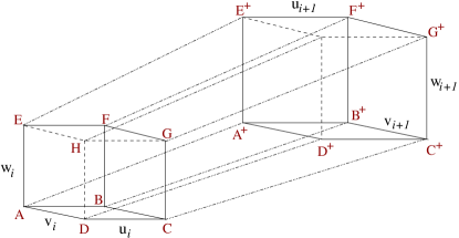
Figure 1: The section of a world-tube joining a rectangular prism to its future counterpart. Homogeneity implies that an observer will fall freely along the centre of the worldtube, providing a convenient coordinate system from which to view the lattice.

The three-geometry is joined to a similar structure at time $t=t_{i+1}=t_{i}+\Delta t_{i}$, where the prisms have edge lengths $u_{i+1}$, $v_{i+1}$ and $w_{i+1}$. This structure is shown in figure 1. Time evolution of the initial surface maintains homogeneity, so within the worldtube of each prism there exists a local freely-falling inertial frame. In the coordinates of this frame the coordinates of vertex $A$ in figure 1 can be written as

$$\left(t_{i},\frac{u_{i}}{2},-\frac{v_{i}}{2},-\frac{w_{i}}{2}\right)$$

and similarly, the coordinates for vertex $A^{+}$ (the counterpart of $A$ on the next hypersurface) are

$$\left(t_{i+1},\frac{u_{i+1}}{2},-\frac{v_{i+1}}{2},-\frac{w_{i+1}}{2}\right).$$

The spacetime interval along the time-like edge joining $A$ and $A^{+}$ is defined to be $m_{i}^{2}<0$, and thus

$$m_{i}^{2}=-\Delta t_{i}^{2}+\frac{1}{4}\left(\Delta u_{i}^{2}+\Delta v_{i}^{2}+\Delta w_{i}^{2}\right),$$ (6)

where the difference operator is defined as $\Delta l_{i}=l_{i+1}-l_{i}$. Note that the requirement that $m_{i}^{2}<0$ implies a restriction on the choice of $\Delta t_{i}$ for a given value of the “resolution” parameter $n$. Homogeneity guarantees that identical expressions hold for all timelike edges joining the spacelike hypersurfaces labeled $t_{i}$ and $t_{i+1}$.

The discrete spacetime curvature in Regge calculus is manifest on the two-dimensional faces on which three-dimensional blocks hinge [1], and is represented by the angle deficit (the difference from the flat space value) measured in the plane orthogonal to the face. There are two distinct classes of two-dimensional faces, or hinges, in the lattice: timelike areas formed by evolving a spacelike edge forward to the next hypersurface, and the rectangular faces of the prisms on $t=\mbox{constant}$ slices.

The timelike trapezoids formed when the spatial edge $u_{i}$ is carried forward in time from the hypersurface labeled $t_{i}$ to $t_{i+1}$, face $ABA^{+}B^{+}$ in figure 1, has area

$$A^{xt}_{i}=\frac{1}{4}\left(u_{i+1}+u_{i}\right)\sqrt{\Delta u_{i}^{2}-4m_{i}^{2}},$$

which is real since $m_{j}^{2}<0$. Likewise, the spacelike hinge $ABCD$ shown in figure 1, consisting of the edges $u_{i}$ and $v_{i}$, has area

$$A^{xy}_{i}=u_{i}v_{i},$$

with the other spacelike and timelike hinges defined similarly.

Turning now to the curvature about these faces, we note that there are four distinct three-dimensional prisms which hinge on the timelike face $ABA^{+}B^{+}$. Each of these is formed by dragging one of the two-dimensional faces containing the edge $AB$ forward in time. This includes the prisms $ABCDA^{+}B^{+}C^{+}D^{+}$ and $ABEFA^{+}B^{+}E^{+}F^{+}$. The remaining two prisms hinging on $ABA^{+}B^{+}$ are not shown in figure 1.

The homogeneity of the lattice ensures that the four hyper-dihedral angles that surround the hinge $ABA^{+}B^{+}$ are the same. Denoting each of these angles as $\theta^{xt}_{i}$, the angle defect (or deficit angle) about the timelike face $ABA^{+}B^{+}$ is

$$\epsilon^{xt}_{i}=2\pi-4\theta^{xt}_{i},$$

which measures the deviation of the total angle from the flat-space value of $2\pi$. The hyper-dihedral angle $\theta^{xt}_{i}$ is

$$\cos\theta^{xt}_{i}=\frac{\Delta v_{i}\Delta w_{i}}{\sqrt{\left(4\Delta t_{i}^{2}-\Delta v_{i}^{2}\right)\left(4\Delta t_{i}^{2}-\Delta w_{i}^{2}\right)}},$$

with analogous definitions for $\theta^{yt}_{i}$ and $\theta^{zt}_{i}$, the hyper-dihedral angles about the remaining classes of spacelike hinge.

To measure the deficit angles about the spacelike faces, consider the curvature $\epsilon^{xy}_{i}$ about the hinge $ABCD$. Since this hinge is spacelike, the hyper-dihedral angles are boosts in the plane with signature $-+$ orthogonal to the hinge. The deficit angle for a spacelike hinge is [16]

$$\epsilon^{xy}_{i}=-\sum_{k}\phi_{k},$$

where the summation is over all boosts $\phi_{k}$ which surround the hinge. The boost between the two three-dimensional prisms which hinge on $ABCD$, namely $ABCDA^{+}B^{+}C^{+}D^{+}$ and $ABCDEFGH$, is

$$\sinh\phi^{xy}_{i}=-\frac{\Delta w_{i}}{\sqrt{4\Delta t_{i}^{2}-\Delta w_{i}^{2}}},$$

and the hinge $ABCD$ is surrounded by four such boosts, two identical boosts above and two below. Thus the final deficit angle measured about $ABCD$ is

$$\epsilon^{xy}_{i}=2\left(\phi^{xy}_{i-1}-\phi^{xy}_{i}\right).$$

Further details on calculating the deficit angles about a spacelike hinge are contained in a recent paper by Brewin [16]. We note that this type of hinge was not included in the calculations of Lewis [7], leading to errors in the resulting Regge equations. We return to this issue below.

4 The Regge calculus model

The vacuum Regge equations take the form [1]

$$0=\sum_{t}\epsilon_{t}\,\frac{\partial A_{t}}{\partial L^{2}_{j}},$$

where the sum is over all triangles $t$ with area $A_{t}$ that contain the edge $L_{j}$, and $\epsilon_{t}$ the deficit angle about triangle $t$. Each edge in the lattice yields a single Regge equation, but the homogeneity and anisotropy of our model imply that there is one distinct equation for each of the four classes of edge in the lattice.

The Regge equation associated with an individual timelike edge $m_{i}^{2}$ involves six timelike lattice faces, and has the form

$$0=2\,\epsilon^{xt}_{i}\,\frac{\partial A^{xt}_{i}}{\partial m^{2}_{i}}+2\,\epsilon^{yt}_{i}\,\frac{\partial A^{yt}_{i}}{\partial m^{2}_{i}}+2\,\epsilon^{zt}_{i}\,\frac{\partial A^{zt}_{i}}{\partial m^{2}_{i}},$$

which is the discrete counterpart of (1), the Einstein field equation $G_{tt}=0$. Similarly, the Regge equation which corresponds to the single spatial edge $u_{i}$ involves six lattice faces: two spacelike faces with area $u_{i}v_{i}$, two with area $u_{i}w_{i}$, plus the timelike faces formed by evolving $u_{i}$ both forwards and backwards in time. The vacuum Regge equation is

$$0=2\,\epsilon^{xy}_{i}\,\frac{\partial A^{xy}_{i}}{\partial u^{2}_{i}}+2\,\epsilon^{xz}_{i}\,\frac{\partial A^{xz}_{i}}{\partial u^{2}_{i}}+\epsilon^{xt}_{i}\,\frac{\partial A^{xt}_{i}}{\partial u_{i}^{2}}+\epsilon^{xt}_{i-1}\,\frac{\partial A^{xt}_{i-1}}{\partial u_{i}^{2}}$$

with similar expressions for the equations arising from the spacelike edges $v_{i}$ and $w_{i}$.

Using the geometric information collected in section 3 we obtain a single Regge equation for each class of edge on the $i$th hypersurface, namely

$$\qquad 0=-\frac{(w_{i}+w_{i+1})\,\epsilon^{{zt}}_{i}}{4\sqrt{\Delta w_{i}^{2}-4m_{i}^{2}}}-\frac{(v_{i}+v_{i+1})\,\epsilon^{{yt}}_{i}}{4\sqrt{\Delta v_{i}^{2}-4m_{i}^{2}}}-\frac{(u_{i}+u_{i+1})\,\epsilon^{{xt}}_{i}}{4\sqrt{\Delta u_{i}^{2}-4m_{i}^{2}}}$$ (7)

$$\qquad 0=v_{i}\epsilon^{xy}_{i}+w_{i}\epsilon^{xz}_{i}+\frac{-2m_{i-1}^{2}+u_{i}\Delta u_{i-1}}{2\sqrt{\Delta u_{i-1}-4m_{i-1}^{2}}}\,\epsilon^{{xt}}_{i-1}+\frac{-2m_{i}^{2}-u_{i}\Delta u_{i}}{2\sqrt{\Delta u_{i}^{2}-4m_{i}^{2}}}\,\epsilon^{xt}_{i}$$ (8)

$$\qquad 0=u_{i}\epsilon^{xy}_{i}+w_{i}\epsilon^{yz}_{i}+\frac{-2m_{i-1}^{2}+v_{i}\Delta v_{i-1}}{2\sqrt{\Delta v_{i-1}-4m_{i-1}^{2}}}\,\epsilon^{{yt}}_{i-1}+\frac{-2m_{i}^{2}-v_{i}\Delta v_{i}}{2\sqrt{\Delta v_{i}^{2}-4m_{i}^{2}}}\,\epsilon^{yt}_{i}$$ (9)

$$\qquad 0=u_{i}\epsilon^{xz}_{i}+v_{i}\epsilon^{yz}_{i}+\frac{-2m_{i-1}^{2}+w_{i}\Delta w_{i-1}}{2\sqrt{\Delta w_{i-1}-4m_{i-1}^{2}}}\,\epsilon^{{zt}}_{i-1}+\frac{-2m_{i}^{2}-w_{i}\Delta w_{i}}{2\sqrt{\Delta w_{i}^{2}-4m_{i}^{2}}}\,\epsilon^{zt}_{i}$$ (10)

which correspond to the lattice edges $m_{j}^{2}$, $u_{j}$, $v_{j}$ and $w_{j}$, respectively.

The structure of the Regge equations (7)-(10) is worth considering. Equation (7), associated with the timelike edge $m_{i}^{2}$, involves edges on, and between, two neighbouring hypersurfaces, whereas (8)-(10) involve information on and between three consecutive spatial hypersurfaces. Thus (7) is a first-order constraint, while (8)-(10) are second-order difference equations.

This contrasts sharply with the equations derived by Lewis [7], who neglected the curvature associated with spacelike hinges, and was thus unable to derive the spatial equations (8)-(10). After correctly obtaining (7), Lewis found that he could only make sense of the truncated spatial equations by considering a careful average. This averaging resulted, once again, in the timelike equation (7). Without the spatial curvature terms $\epsilon^{yz}_{i}$, $\epsilon^{xz}_{i}$ and $\epsilon^{xy}_{i}$ Lewis was unable to build the second-order Regge equations (8)-(10).

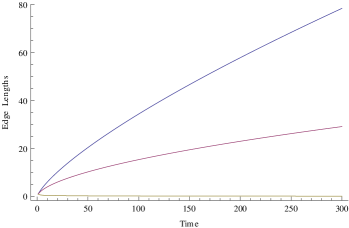
(a) Evolution of edge lengths

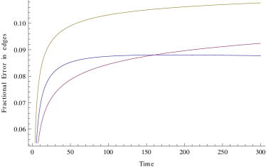
(b) Fractional error in edge lengths

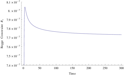
(c) Time evolution of the constraint $R_{t}$

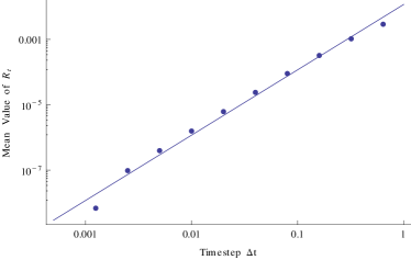
(d) Convergence of the mean value of $R_{t}$

Figure 2: Discrete Regge solutions with $p_{1}=0.75$ and $\Delta t=0.01$.

Before examining the continuum limit of the Regge model we consider solutions of the discrete equations. Initial data is constructed at $t_{0}=1$ to match the continuum Kasner solution as far as possible. Taking the exact initial data to be $x(1)=y(1)=z(1)=1$ and $\dot{x}(1)=p_{1}$, $\dot{y}(1)=p_{2}$, and $\dot{z}(1)=p_{3}$, we mimic the properties of the exact solution in the lattice by setting $u_{0}=v_{0}=v_{0}=1$ and

$$\qquad u_{1}=u_{0}+(p_{1}+\alpha)\,\Delta t,\qquad v_{1}=v_{0}+(p_{2}+\alpha)\,\Delta t,\qquad w_{1}=w_{0}+(p_{3}-2\alpha)\,\Delta t$$

where $\alpha$ is an unknown parameter. This form is chosen to maintain the continuum condition $\dot{x}(1)+\dot{y}(1)+\dot{z}(1)=1$ to first order, which is physically equivalent to using the degrees of freedom in the initial data to generate linear expansion in the volume element. With these initial data the Regge constraint (7) is solved for the single parameter $\alpha$.

A typical solution of the discrete Regge equations is shown in figure 2 for the case $p_{1}=0.75$ and $\Delta t=0.01$. The solution to the initial value problem in this case is $\alpha=0.0214379$, which represents a roughly $3\%$ change in the initial rate of change of $u_{i}$ compared to the exact estimate. The evolution of the initial data is shown in figure 2a, while 2b shows the evolution of the fractional error in the Regge solutions compared with their exact counterparts. The fractional error in all edges remains in the $5\%-10\%$ range, and can be shown to shrink as the time step is reduced.

The residual error in the first-order Regge constraint (7) is defined as

$$R_{t}=\frac{(w_{i}+w_{i+1})\,\epsilon^{{zt}}_{i}}{4\sqrt{\Delta w_{i}^{2}-4m_{i}^{2}}}+\frac{(v_{i}+v_{i+1})\,\epsilon^{{yt}}_{i}}{4\sqrt{\Delta v_{i}^{2}-4m_{i}^{2}}}+\frac{(u_{i}+u_{i+1})\,\epsilon^{{xt}}_{i}}{4\sqrt{\Delta u_{i}^{2}-4m_{i}^{2}}},\\$$ (11)

and is a measure of the consistency amongst the Regge equations. Figure 2c shows $R_{t}$ as a function of time with $\Delta t=0.01$, and clearly the residual $R_{t}$ remains small throughout the evolution. We repeated this process with different $\Delta t$ to estimate the rate at which $R_{t}$ reduces as $\Delta t$ tends to zero. Figure 2d shows second-order convergence in the mean value of $R_{t}$ over $1<t<100$ as the timestep is reduced. We explore the issue of convergence in more detail in the following sections.

5 The continuous-time Regge model

Many of the early applications of Regge calculus to highly symmetric spacetimes considered the differential equations that arise in the limit of continuous time and discrete space [7, 8, 9]. In this section we derive the continuous time Regge equations and compare them with the results of Lewis [7] before considering numerical solutions.

The continuous-time Regge model is developed from the discrete equations in section 4 in the limit of small $\Delta t$, with the assumption that spatial edges in the lattice approach continuous functions of time. For example, the spacelike edge $u_{i}$ is viewed as the value of a continuous function $u(t)$ evaluated at $t=t_{i}$. A power series expansion then relates the edge lengths on neighbouring surfaces,

$$u_{i+1}=u(t_{i})+\frac{\partial u}{\partial t}\Delta t+\frac{1}{2}\frac{\partial^{2}u}{\partial t^{2}}\Delta t^{2}+\frac{1}{6}\frac{\partial^{3}u}{\partial t^{3}}\Delta t^{3}+{\Or}(\Delta t^{4}),$$ (12)

where all derivatives are evaluated at $t=t_{i}$. Similar expressions hold for the edges $u_{i-1},v_{i+1}$ etc. The series expansion for the timelike edges $m_{i}^{2}$ is obtained from (6).

In the continuum limit the deficit angle about the spacelike area $A^{xy}_{i}$ is

$$\epsilon_{xy}(t) = \frac{4\ddot{u}}{4-\dot{u}^{2}}\,\Delta t+\Or(\Delta t^{3}),$$

and the deficit angle about the timelike face formed by the evolution of $u_{i}$ is

$$\epsilon_{xt}(t) = 2\pi-4\cos^{-1}\left(\frac{\dot{v}\,\dot{w}}{\sqrt{(4-\dot{v}^{2})(4-\dot{w}^{2})}}\right)+\Or(\Delta t),$$

with similar expressions for the remaining faces.

Using these expansions, the Regge equations (7)-(10) are, to leading order,

$$\quad 0=-\left[\frac{u\,\epsilon_{xt}^{0}}{\sqrt{4-\dot{v}^{2}-\dot{w}^{2}}}+\frac{v\,\epsilon_{yt}^{0}}{\sqrt{4-\dot{u}^{2}-\dot{w}^{2}}}+\frac{w\,\epsilon_{zt}^{0}}{\sqrt{4-\dot{u}^{2}-\dot{v}^{2}}}\,\right]+\Or(\Delta t)$$ (13)

$$\quad 0=\left[\,\frac{4w\ddot{v}}{4-\dot{v}^{2}}+\frac{4v\ddot{w}}{4-\dot{w}^{2}}-\frac{4u\dot{u}}{4-\dot{v}^{2}-\dot{w}^{2}}\left(\frac{\ddot{v}\dot{w}}{4-\dot{v}^{2}}+\frac{\dot{v}\ddot{w}}{4-\dot{w}^{2}}\right)\right.$$ (14)

$$\left.\quad+\,\frac{\epsilon^{0}_{xt}\,\left(4-\dot{u}^{2}-\dot{v}^{2}-\dot{w}^{2}-u\ddot{u}\right)}{2\sqrt{4-\dot{v}^{2}-\dot{w}^{2}}}-\frac{\epsilon^{0}_{xt}\,u\dot{u}\left(\dot{v}\ddot{v}+\dot{w}\ddot{w}\right)}{2\left(4-\dot{v}^{2}-\dot{w}^{2}\right)^{3/2}}\,\,\right]\Delta t+\Or(\Delta t^{3})$$

$$\quad 0=\left[\,\frac{4w\ddot{u}}{4-\dot{u}^{2}}+\frac{4u\ddot{w}}{4-\dot{w}^{2}}-\frac{4v\dot{v}}{4-\dot{u}^{2}-\dot{w}^{2}}\left(\frac{\ddot{u}\dot{w}}{4-\dot{u}^{2}}+\frac{\dot{u}\ddot{w}}{4-\dot{w}^{2}}\right)\right.$$ (15)

$$\left.\quad+\,\frac{\epsilon^{0}_{yt}\left(4-\dot{u}^{2}-\dot{v}^{2}-\dot{w}^{2}-v\ddot{v}\right)}{2\sqrt{4-\dot{u}^{2}-\dot{w}^{2}}}-\frac{\epsilon^{0}_{yt}v\dot{v}\left(\dot{u}\ddot{u}+\dot{w}\ddot{w}\right)}{2\left(4-\dot{u}^{2}-\dot{w}^{2}\right)^{3/2}}\,\,\right]\Delta t+\Or(\Delta t^{3})$$

$$\quad 0=\left[\,\frac{4v\ddot{u}}{4-\dot{u}^{2}}+\frac{4u\ddot{v}}{4-\dot{v}^{2}}-\frac{4w\dot{w}}{4-\dot{u}^{2}-\dot{v}^{2}}\left(\frac{\ddot{u}\dot{v}}{4-\dot{u}^{2}}+\frac{\dot{u}\ddot{v}}{4-\dot{v}^{2}}\right)\right.$$ (16)

$$\left.\quad+\,\frac{\epsilon^{0}_{zt}\left(4-\dot{u}^{2}-\dot{v}^{2}-\dot{w}^{2}-w\ddot{w}\right)}{2\sqrt{4-\dot{u}^{2}-\dot{v}^{2}}}-\frac{\epsilon^{0}_{zt}\,w\dot{w}\left(\dot{u}\ddot{u}+\dot{v}\ddot{v}\right)}{2\left(4-\dot{u}^{2}-\dot{v}^{2}\right)^{3/2}}\,\,\right]\Delta t+\Or(\Delta t^{3})$$

where $\epsilon^{0}_{xt},\epsilon^{0}_{yt}$ and $\epsilon^{0}_{zt}$ denote the zeroth order terms in the deficit angle expansions. The leading terms in (13)-(16) are the continuous-time Regge equations, a set of non-linear differential equations. Equation (13) is a first-order differential equation, while the remainder are second-order.

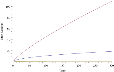
(a) Evolution of edge lengths

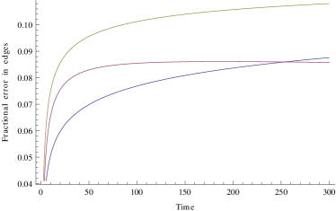
(b) Fractional error in edge lengths

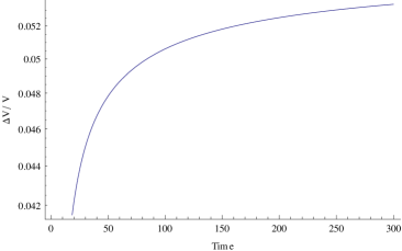
(c) Fractional error in prism volume

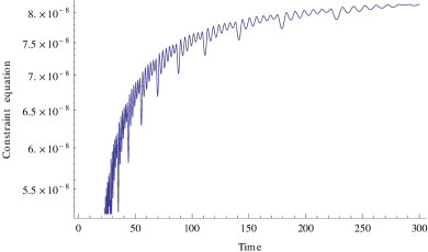
(d) Residual in the constraint (13)

Figure 3: Solution of the continuous-time Regge differential equations with $p_{1}=0.5$.

The continuous-time Regge differential equations were solved numerically using Mathematica. Initial conditions were applied at $t_{0}=1$, and the initial data was chosen to ensure that the expansion of lattice volume elements is initially linear to match the exact solution in section 2. Once again introducing a parameter $\alpha$, we set

$$u(1)=v(1)=w(1)=1\qquad\mbox{and}$$

$$\dot{u}(1)=p_{1}+\alpha,\qquad\dot{v}(1)=p_{2}+\alpha,\qquad\dot{w}(1)=p_{3}-2\alpha,$$

and use the first-order Regge initial value equation (13) to solve for $\alpha$. This mimics the exact initial data, for which $\alpha=0$. The second-order, non-linear differential equations (14)-(16) are used to evolve the initial data forward in time.

Figure 3 shows solutions to the continuous-time Regge equations with $p_{1}=0.5$. The solution to the initial value problem is $\alpha=0.0204161$, which represents a small deviation ($\approx 4\%$ change in the initial value of $\dot{u}$) from the exact initial data. As can be seen in the figure, the continuous-time Regge solutions are very similar to the exact Einstein solution, with the Regge edges deviating from the exact values by $5\%-7\%$. In the next section we extend the limiting process to the spatial edges, and examine the difference between the exact and Regge equations more carefully.

6 The Regge equations in the limit of continuous space and time

In this section we explore the discrepancies between the discrete Regge model and the Kasner spacetime by examining the truncation error incurred when the Regge equations are viewed as approximations of the Kasner-Einstein equations (1)-(4). We consider the continuum limit of the Regge equations (7)-(10) as the spatial lattice is refined in both space and time.

The continuous space and time limit of the Regge equations is obtained from the temporal series expansions (12) together with the link between lattice edges and the global length scales given by (5). Substituting these into the discrete Regge equations (7)-(10) and simultaneously increasing the number of prisms ($n\rightarrow\infty$) while reducing the timestep ($\Delta t\rightarrow 0$) we obtain a series expansion for the the discrete equations in the continuum limit. The refinement parameter $n$ and timestep $\Delta t$ are chosen so that $m_{j}^{2}<0$.

The series expansion of the temporal Regge equation (7) is

$$\qquad 0=\frac{-1}{2n^{3}}\left[\left(x\frac{dy}{dt}\frac{dz}{dt}+y\frac{dx}{dt}\frac{dz}{dt}+z\frac{dx}{dt}\frac{dy}{dt}\right)\right.$$ (17)

$$\left.\quad+\,\frac{1}{2}\left(\ 3\,\frac{dx}{dt}\frac{dy}{dt}\frac{dz}{dt}+z\frac{dy}{dt}\frac{d^{2}x}{dt^{2}}+y\frac{dz}{dt}\frac{d^{2}x}{dt}+z\frac{dx}{dt}\frac{d^{2}y}{dt}\right.\right.$$

$$\left.\left.\qquad\qquad+\ x\frac{dz}{dt}\frac{d^{2}y}{dt}+y\frac{dx}{dt}\frac{d^{2}z}{dt}+x\frac{dy}{dt}\frac{d^{2}z}{dt}\right)\,\Delta t+{\Or}(\Delta t^{2},\frac{1}{n^{2}})\right],$$

which has truncation error that is first-order in the timestep $\Delta t$ and second-order in the spatial discretization scale $1/n$. The spatial Regge equations (8)-(10) are

$$\frac{\Delta t}{n^{2}}\left\{\frac{dy}{dt}\frac{dz}{dt}+y\frac{d^{2}z}{dt^{2}}+z\frac{d^{2}y}{dt^{2}}+{\Or}(\Delta t^{2},\frac{1}{n^{2}})\right\}=0$$ (18)

$$\frac{\Delta t}{n^{2}}\left\{\frac{dx}{dt}\frac{dz}{dt}+x\frac{d^{2}z}{dt^{2}}+z\frac{d^{2}x}{dt^{2}}+{\Or}(\Delta t^{2},\frac{1}{n^{2}})\right\}=0$$ (19)

$$\frac{\Delta t}{n^{2}}\left\{\frac{dx}{dt}\frac{dy}{dt}+x\frac{d^{2}y}{dt^{2}}+y\frac{d^{2}x}{dt^{2}}+{\Or}(\Delta t^{2},\frac{1}{n^{2}})\right\}=0$$ (20)

to leading order in the continuum limit. The truncation error in these equations is second order in both the spatial and temporal discretization scales.

The leading order terms in the continuous time and space Regge equations (17)-(20) are identical to the Kasner-Einstein equations (1)-(4), so we expect solutions of the discrete lattice equations to approach the continuum solutions as length scales in the lattice are reduced. It is clear from the preceding equations that the truncation error for the Regge equations, when viewed as approximations to the Kasner-Einstein equations, are second order in the spatial discretization scale $1/n$. The truncation error is also second order in $\Delta t$ for the spatial Regge equations (18)-(20).

The truncation error in (17) implies that the Regge initial value equation (7) is only a first-order approximation to its continuum counterpart. This conflicts with the calculations in section 4, where the truncation error in the Regge constraint $R_{t}$ was found to converge to zero as the second power of $\Delta t$ (see figure 2d). To understand this contradiction, we rewrite the coefficients of $\Delta t$ in the expansion (17) as

$$\quad 3\,\dot{x}\dot{y}\dot{z}+\dot{y}\left(z\ddot{x}+x\ddot{z}\right)+\dot{z}\left(y\ddot{x}+x\ddot{y}\right)+\dot{x}\left(z\ddot{y}+y\ddot{z}\right)$$

$$=\dot{x}\left(\dot{y}\dot{z}+z\ddot{y}+y\ddot{z}\right)+\dot{y}\left(\dot{x}\dot{z}+z\ddot{x}+x\ddot{z}\right)+\dot{z}\left(\dot{y}\dot{z}+y\ddot{x}+x\ddot{y}\right)$$

$$=0+{\Or}(\Delta t^{2},\frac{1}{n^{2}}),$$

where the final equality follows from substitution of (18)-(20). Thus the truncation error in the Regge constraint (17) is formally of order $\Delta t$, but the coefficient of that term in the expansion is a linear combination of the spatial Kasner-Einstein equations. This should be zero to leading order for any solution of the spatial Regge equations.

To clarify this argument, consider again the simulation in section 4. Once the initial data is set, the numerical evolution is achieved by the repeated solution of the spatial Regge equations (8)-(10). These are shown above to be second order accurate approximations of the Einstein equations in both space and time. We expect from (17) that the leading order error in the Regge constraint is first order in $\Delta t$. However, the coefficient of that error term is a linear combination of the Regge equations we are solving (to leading order), and thus the coefficient of $\Delta t$ is itself zero to second order in $\Delta t$. Thus the effective leading order truncation in the Regge constraint equation (17) is of second order in both space and time. This is consistent with the numerical experiments in section 4.

7 Discussion

In the preceding sections we re-examined one of the most highly symmetric applications of Regge calculus to be found in the literature. The primary goal of this study was to examine the convergence properties of Regge calculus, and we have shown that for the discrete Kasner spacetime the equations of Regge calculus reduce identically to the corresponding Einstein equations in the continuum limit.

The discrete lattice used by Lewis, outlined above, was specifically designed to guarantee a one-to-one correspondence between the degrees of freedom in the Regge lattice and the metric components in the continuum solution [7]. Despite this, Lewis needed to average the Regge evolution equations in order to obtain consistency in the continuum limit. The averaging process was chosen to obtain the first order Regge equation (7), but Lewis was still unable to derive the remaining spatial equations (8)-(10). We showed in section 4 that once all lattice curvature elements are included in the calculations the Regge equations consist of one constraint and three evolution equations. In section 6 we showed that these lattice equations approach the full set of Kasner-Einstein equations in the continuum limit.

It was also shown in section 6 that the discrete Regge equations are second order accurate approximations to the Einstein equations for the Kasner cosmology in the limit of very fine discretization. This convergence rate is in agreement with many previous numerical simulations, in particular the (3+1)-dimensional Regge calculus models of the Kasner cosmology that utilized general simplicial lattices [10, 19]. Unlike the current analysis, these simulations did not enforce the homogeneity and anisotropy of the Kasner model throughout the evolution, yet displayed second-order convergence to the continuum solution. These numerical simulations considered the convergence of solutions, rather than equations, and so are complementary to our analysis.

In general applications of Regge calculus that utilize a simplicial lattice there will be many more Regge equations (one per lattice edge) than Einstein equations (10 per spacetime event). The direct comparison between individual Regge and continuum equations considered in this paper would not be possible, or even desirable. We expect that an appropriate average of the Regge equations would still correspond to the Einstein equations in the continuum limit [17, 18, 20], and several such averaging schemes have been suggested. Brewin considered a finite-element integration of the weak-field Einstein equations over a simplicial lattice (discussed in [18]), and suggested that the vertex-based equivalent of the vacuum Einstein equations are

$$0=\sum_{j}\sum_{i(j)}(\Delta x^{\mu}\Delta x^{\nu})_{i}\,\epsilon_{j}\,\frac{\partial A_{j}}{\partial L^{2}_{i}},$$

where $\Delta x^{\mu}_{j}$ is a vector oriented along edge $L_{j}$ in a coordinate system based at vertex $v$. The outer summation is over all triangles which meet at $v$, and the inner sum is over the edges on each triangle. These are essentially linear combinations of Regge equations, together with boundary terms [18].

Regardless of how one compares the continuum and discrete equations, it is ultimately the solutions that are of interest. The application of Regge calculus to the Kasner cosmology discussed in this paper demonstrates yet again that Regge calculus is a consistent second-order accurate discretization of general relativity, providing further support for the use of lattice gravity in numerical relativity and discrete quantum gravity.

References

References

- [1] Regge T 1961 Nuovo Cimento19 558–71
- [2] Williams R M and Tuckey P A 1992 Class. Quantum Grav.9 1409–22
- [3] Regge T and Williams R M 2000 J. Math. Phys.41 3964–84
- [4] Gentle A P 2002 Gen. Rel. Grav. 34 1701–-18
- [5] Alsing P M, McDonald J R and Miller W A 2011 Class. Quantum Grav.28 155007
- [6] Stuckey W M, McDevitt T J and Silberstein M 2011 Modified Regge calculus as an explanation of dark energy Preprint arXiv.org:1110.3973
- [7] Lewis S M 1982 Phys. Rev.D25 306–12
- [8] Collins P A and Williams R M 1973 Phys. Rev.D7 965–71
- [9] Brewin L C 1987 Class. Quantum Grav.4 899–928
- [10] Gentle A P and Miller W A 1998 Class. Quantum Grav.15 389–405
- [11] Kasner E 1921 Amer. Jour. Math. XLIII 217–21
- [12] Misner C, Thorne K S and Wheeler J A 1973 Gravitation W. H. Freeman and Co.
- [13] Belinsky V A, Khalatnikov I M and Lifshitz E M 1970 Adv. Phys. 19 525–73
- [14] Cornish N J and Levin J 1997 Phys. Rev. Lett.78 998–1001
- [15] Berger B 2002 Living Rev. Relativity 5 1 [Online Article]: cited on July 30 2012 http://www.livingreviews.org/Articles/Volume5/2002-1berger/
- [16] Brewin L C 2011 Class. Quantum Grav.28 185005
- [17] Miller W A 1986 Found. Phys. 16 143–69
- [18] Brewin L C 2000 Gen. Rel. Grav. 32 897-918
- [19] Brewin L C and Gentle A P 2001 Class. Quantum Grav.18 517–26
- [20] Cheeger J, Müller W and Schrader R 1984 Comm. Math. Phys. 92 405–54