Abstract

We study the spatial distribution of clusters associated to the aftershocks of the megathrust Maule earthquake $M_{W}$ 8.8 of 27 February 2010. We used a recent clustering method which hinges on a nonparametric estimation of the underlying probability density function to detect subsets of points forming clusters associated with high density areas. In addition, we estimate the probability density function using a nonparametric kernel method for each of these clusters. This allows us to identify a set of regions where there is an association between frequency of events and coseismic slip. Our results suggest that high coseismic slip spatially correlates with high aftershock frequency.

Key words: Nonparametric clustering, Kernel density estimation, Maule 2010 Earthquake, aftershock distribution, slip model.

Short title: Nonparametric assessment of Maule earthquake.

1 Introduction

The most recent large Chilean earthquake occurred on February 27th, 2010 ($M_{w}$ = 8.8) and propagated northward and southward achieving a rupture length of about 450 km (35–$37^{\circ}$S; e.g., Lay et al., 2010). The earthquake filled a seismic gap (Ruegg et al., 2009) that has experienced little seismic activity since 1835, when it broke with an estimated magnitude of $M_{w}\sim$8.5 (Darwin, 1851).

Moreno et al. (2010) showed that the two regions of high coseismic slip of the Maule earthquake appeared to be highly locked before the earthquake. Subsequent geodetic studies have established that the main coseismic slip patch ($>$15 m) is located in the northern part of the rupture area, with a secondary concentration of slip to the south (5-12 m) (e. g. Lay et al., 2010; Delouis et al., 2010; Lorito et al. 2011; Vigny et al., 2011; Moreno et al., 2012). Lorito et al. (2011) concluded that increased stress on the unbroken southern patch may have increased the probability of another great earthquake there in the near future, but his model has poor resolution on this area. In addition, Moreno et al. (2012) suggests that coseismic slip heterogeneity at the scale of single asperities appear to indicate seismic potential for future great earthquakes. These studies are not limited to geodetic data, seismic and tsunami data have been used as well in those studies.

The aim of the present work is to examine the spatial correlation between areas of high coseismic slip and the aftershock frequency (seismic clusters). To achieve this, we identify the distribution of clusters in the rupture area of the 2010 earthquake. The hypocenter data are taken from the SSN (Servicio Sismologico Nacional de Chile), and we use the coseismic model of Moreno et al. (2012), which includes all available geodetic data for the Maule earthquake. We adopted the NPC formulation of Azzalini & Torelli (2007), which has the advantage of not requiring the input of some subjective choices such as the number of existing clusters. We apply this methodology to the SSN aftershock catalogue data of the Maule earthquake and focus on the data of the area between Valparaíso and Tirúa [33-38$\mbox{.}5^{\circ}$S], aiming the identification of seismic clusters and its spatial relationship with regions of coseismic slip. Finally, we discuss the possible improvements of the adopted methodology in terms of available geophysical data.

2 Methodology

Applications of clustering techniques range over an enormous set of disciplines, both in the natural sciences (see e.g, Contreras-Reyes & Arellano-Valle, 2012) and in the social sciences (see e.g, Azzalini & Torelli, 2007; Menardi, 2010). A standard account is the book of Kaufman & Rousseeuw (1990), which is focused mainly on the more classical methods, based of the notion of distance between objects. An alternative, more recent approach is the model-based clustering formulation which regards the observed data as generated by a probability distribution a mixture of multivariate random variables having distribution belonging to some parametric family. More specifically, for any point $x$ in the multivariate set of possible observations, we associate a probability density function $f(x)$ and assume that a decomposition of type

$$f(x)=\sum_{j=1}^{J}p_{j}f_{j}(x)$$

exists, where the $p_{j}$’s are mixing probabilities and $f_{j}(x)$ denotes the $j$-th component of the mixture, which also corresponds to the $j$-th cluster of points, for $j=1,\dots,J$. In the implementation of this approach, the most common option is to adopt the multivariate Gaussian assumption for each of the components $f_{j}(x)$, and estimate their parameters using an EM-type algorithm. An especially useful account to this approach is provided by Dasgupta & Raftery (1998). By applying the model-based clustering approach to earthquake data in the coastal area of central California, Dasgupta & Raftery (1998) have obtained six clusters, some of which are clearly linked to active faults, such as San Andreas, Calveras and Hayward faults; however one or two of their clusters do not correspond to some already identified area.

In a further approach to the clustering problem, the notion of an underlying density function $f(x)$ is retained, but the assumption that $f(x)$ is a mixture of components is removed, and so also the connected parametric assumption of the components. Therefore, this approach is based on the construction of a nonparametric estimate $\hat{f}(x)$ of $f(x)$, and the association of a cluster to each of the observed modes of the density. Several alternative formulations of this approach exists (see e.g., Botev et al., 2010; Zhu, 2013), but we concentrate on the kernel-type estimate which is the most popular and conceptually very intuitive (Bowman & Azzalini, 1997). In the univariate case, the kernel estimate is defined by

$$\hat{f}(x)=\frac{1}{n}\sum_{i=1}^{n}\varphi(x-x_{i};h),$$ (1)

where $\varphi(z;h)$ denotes the normal density function with mean $0$ and standard deviation $h$ evaluated at point $z$. The normal density is adopted for simplicity and it could be replaced by another density symmetric about $0$ without much effect on the outcome. A much more important role is played by $h$ which in this context is called ‘smoothing parameter’. In the $d$-dimensional case, $\varphi(z;h)$ is replaced by a multivariate density with a $0$ mean vector; the simplest and most popular choice is the product of $d$ such terms, with a different smoothing parameter for each of the $d$ components. Clusters are then formed by the data points associated to the modes of $\hat{f}(x)$, and the clusters are separated by regions of low density of points. This logic procedure is referred as a nonparametric clustering (NPC).

2.1 Nonparametric clustering

We describe briefly the NPC method proposed by Azzalini & Torelli (2007). This works by assuming that the available set of $d$-dimensional observations $S=\{x_{1},\dots,x_{n}\}$ represent a set of points drawn from a continuous multivariate random variable having an unknown probability density function $f(x)$, $x\in\mathbb{R}^{d}$. In the case we are concerned with, $x=(\mathrm{latitude},\mathrm{longitude})$ denotes a geographical position, hence $d=2$; the data points $x_{1},\dots,x_{n}$ represent the positions of the observed seismic events.

For any given constant $\alpha$ such that $0\leq\alpha\leq\max_{x}f(x)$, consider the high density region defined by

$$R_{\alpha}=\{x:\mbox{ }x\in\mathbb{R}^{2},\mbox{ }f(x)\geq\alpha\}$$ (2)

which has an associated probability $p_{\alpha}=\int_{R_{\alpha}}f(x)\,\mathrm{d}{x}$. The region $R_{\alpha}$ is, in general, formed by a number $m$ of connected sets, where $m\in\{1,2,\dots\}$.

Now we let $\alpha$ moves along its range. This causes both $m$ and $p=p(\alpha)$ to move accordingly, and we can regard $m$ as a function of $p$ since $p$ is monotonic with respect to $\alpha$, write $m(p)$. Note that $m(p)$ is instead a not monotonic function. With the additional conventional settings $m(0)=m(1)=0$, it can be shown that the total number of increments of the step function $m(p)$ is equal to the number $M$ of modes of $f(x)$, hence to the number of clusters, in the sense defined earlier. As $\alpha$ varies along its range, and so does $p(\alpha)$, the corresponding connected components of $R(\alpha)$ form a hierarchical tree structure.

Translating the above idea into a working methodology requires some additional specifications and algorithmic work. We sketch here the main step of the procedure. Full details of the method are given by Azzalini & Torelli (1997) and its implementation in the language R is provided by Azzalini et al. (2011). This procedure will later referred to as the ‘pdfCluster method’.

1. A nonparametric estimate $\hat{f}(x)$ of the density is obtained from the observed sample $S$. Any sort of nonparametric estimate can be employed but in practice both by Azzalini & Torelli (1997) and pdfCluster adopt a kernel-type estimate. This involves to choose a set of kernel bandwidths, one for each component of $x$. When the target is the estimation of the density itself, the outcome depends critically on the choice of the bandwidth. However in the present context, where $\hat{f}(x)$ is only an intermediate step toward the final target of clustering, the bandwidth is much less influential and its choice can be varied over a quite wide range without affecting the end result.

2. For any $\alpha$ in the range $0\leq\alpha\leq\max_{i}\hat{f}(x_{i})$, it considers the sample analogue of (2) given by

   $$S_{\alpha}=\{x_{i}:~{}x_{i}\in S,~{}\hat{f}(x_{i})\geq\alpha\}\,.$$ (3)

   The notion of connected subsets of $S_{\alpha}$ is introduced via the notion of Delaunay triangulation which is built by making use of computational geometry tools. This leads to establish a certain set of line segments joining some of the data points in such a way that, for any two data points, there always exists a path joining them by a sequence of these segments. If $x_{r}$ and $x_{s}$ are both points in $S_{\alpha}$ and the path joining them does not include any point outside $S_{\alpha}$, then we say that $x_{r}$ and $x_{s}$ are connected, at the given choice of $\alpha$.

3. The above step is replicated for a grid of values spanning the admissible range of $\alpha$, from $0$ to $\max_{i}\hat{f}(x_{i})$. This generates a mode function $\hat{m}(p)$ and a tree structure of the modes. Notice however that the Delaunay triangulation needs to be determined only once for all $\alpha$’s.

4. At the end of the earlier step we have obtained a tree structure of the modes of $\hat{f}(x)$. Moreover, for each of the $M$ modes, we have allocated some elements of the sample $S$ to the given mode. These $M$ subsets of data points form the ‘cluster cores’ to which the remaining points, not belonging to any cluster core, must be aggregated. For each unallocated point $x_{0}$, we must select one of distributions $\hat{f}_{1}(x),\dots,\hat{f}_{M}(x)$ which represent the estimated densities of the cluster cores. This allocation is most naturally based on the likelihood ratio, that is we allocate $x_{0}$ to the $j$-th cluster core such that the ratio

   $$\frac{\hat{f}_{j}(x_{0})}{\max_{k\neq j}\hat{f}_{k}(x_{0})}$$

   is highest. In practice, there are some variant options, depending on whether the $\hat{f}_{j}(x)$ densities of the cluster cores are updated at each new allocation or not, or according to some intermediate strategy.

The final outcome of the clustering process is represented by the a partition of the sample $S$ into a set of clusters, say $C_{1},\dots,C_{M}$.

2.2 Density-based silhouette diagnostic

In cluster analysis, the term ‘silhouette’ refers to a diagnostic tool for the validation of the outcome of the clustering process (Rousseeuw, 1987). This technique provides a graphical representation of how well each object spatially lies within a cluster to which it has been allocated; hence it provides an indication of how appropriately the data has been clustered. The idea arises from the comparison of the small distance of each observation to the cluster where it has been allocated and a measure of separation from the closest alternative cluster.

Since the original silhouette is based on a distance measure between the observations, it is not adequate for NPC methods where distances do not play an explicit role. An adaption of the silhouette idea to density-based clustering methods has been proposed by Menardi (2010). The method, called density-based silhouette (DBS) diagnostic, is based on the posterior probabilities

$$p_{j}(x_{i})=\frac{\hat{\pi}_{j}\hat{f}_{j}(x_{i})}{\sum_{j=1}^{M}\hat{\pi}_{j}\hat{f}_{j}(x_{i})},\qquad j=1,\dots,M,$$

where $\hat{\pi}_{j}$ plays the role of prior probability of cluster $C_{j}$; in practice it is taken to be the proportion of points allocated to $C_{j}$. The DBS index of observation $x_{i}$ is

$$\mathrm{dbs}(x_{i})=\frac{\hbox{log}\left(\frac{p_{j_{0}}(x_{i})}{p_{j_{1}}(x_{i})}\right)}{\max_{k=1,...,n}\left|\hbox{log}\left(\frac{p_{j_{0}}(x_{k})}{p_{j_{1}}(x_{k})}\right)\right|}$$

where $j_{0}$ denotes the cluster to which $x_{i}$ has been allocated, and $j_{1}$ refers to the alternative cluster index for which $p_{j}$ is maximum, $j\neq j_{0}$.

In our case, after partitioning the SSN data with the pdfCluster method, we applied the DBS diagnostic to assess the quality of the outcome.

2.3 Temporal analysis

We briefly describe four indexes to illustrate the consistency of the NPC method across the time. These indexes perform accuracy of the observed in predicting the corrected category, relative to that of random chance. In Table 1, $n(F_{i},O_{j})$ denotes the number of forecasts in category $i$ that had observations in category $j$, $N(F_{i})$ denotes the total number of forecasts in category $i$, $N(O_{j})$ denotes the total number of observations in category $j$, $N$ is the total number of forecasts and $i,j=1,...,5$ are the indexes of the five identified clusters.

$$NSS = \frac{1}{N}\sum_{i=1}^{5}N(F_{i},O_{i}),$$

$$HSS = \frac{NSS-\frac{1}{N^{2}}\sum_{i=1}^{5}N(F_{i})N(O_{i})}{1-\frac{1}{N^{2}}\sum_{i=1}^{5}N(F_{i})N(O_{i})},$$

$$HK = \frac{N^{2}-\sum_{i=1}^{5}N(F_{i})N(O_{i})}{N^{2}-\sum_{i=1}^{5}N(O_{i})^{2}}HSS$$

where $NSS$ corresponds to normal skill score with range $[0,1]$, such that 0 indicates no skill, and 1 indicates perfect score. The index $HSS$ correspond to Heidke skill score (Brier & Allen, 1952) with range $(-\infty,1]$, 0 indicates no skill, and 1 indicates perfect score.

Table 1: Multi-category Contingence table with five clusters.

Observed Category
		1	2	3	4	5	Total
	1	$n(F_{1},O_{1})$	$n(F_{1},O_{2})$	$n(F_{1},O_{3})$	$n(F_{1},O_{4})$	$n(F_{1},O_{5})$	$N(F_{1})$
	2	$n(F_{2},O_{1})$	$n(F_{2},O_{2})$	$n(F_{2},O_{3})$	$n(F_{2},O_{4})$	$n(F_{2},O_{5})$	$N(F_{2})$
Forecast	3	$n(F_{3},O_{1})$	$n(F_{3},O_{2})$	$n(F_{3},O_{3})$	$n(F_{3},O_{4})$	$n(F_{3},O_{5})$	$N(F_{3})$
Category	4	$n(F_{4},O_{1})$	$n(F_{4},O_{2})$	$n(F_{4},O_{3})$	$n(F_{4},O_{4})$	$n(F_{4},O_{5})$	$N(F_{4})$
	5	$n(F_{5},O_{1})$	$n(F_{5},O_{2})$	$n(F_{5},O_{3})$	$n(F_{5},O_{4})$	$n(F_{5},O_{5})$	$N(F_{5})$
Total		$N(O_{1})$	$N(O_{2})$	$N(O_{3})$	$N(O_{4})$	$N(O_{5})$	$N$

The index $HK$ correspond to Hanssen & Kuipers discriminant (Hanssen & Kuipers, 1965) with range $[-1,1]$, such that 0 indicates no skill, and 1 indicates perfect score. Similar to the Heidke skill score, except that in the denominator the fraction of correct forecasts due to random chance is for an unbiased forecast. Hubert & Arabie (1985) noticed that the Rand index is not corrected for chances that are equal to zero and for random partitions having the same number of objects in each class. They introduced the corrected Rand index, whose expectation is equal to zero. The adjusted Rand index is based on three values: the number $r$ of common joined pairs in O and F, the expected value $E(r)$ and the maximum value $\max(r)$ of this index, among the partitions of the same type as O and F. It leads to the formula

$$HA(O,F)=\frac{r-E(r)}{\max(r)-E(r)}$$

where

$$r=\sum_{i=1}^{5}\sum_{j=1}^{5}\frac{n_{i,j}(n_{i,j}-1)}{2}, E(r)=\frac{1}{2}\frac{|N(O)|\times|N(F)|}{n(n-1)}\,,$$

$$|N(O)|=\sum_{i=1}^{5}\frac{n_{i}(n_{i}-1)}{2}, |N(F)|=\sum_{j=1}^{5}\frac{n_{j}(n_{j}-1)}{2}$$

and $\max(r)=\frac{1}{2}(|N(O)|+|N(F)|)$. This maximum value is questionable since the number of common joined pairs is necessarily bounded by $\inf{\{|N(O)|,|N(F)|\}}$, but $\max(r)$ insures that the maximum value of $HA$ is 1 when the two partitions are identical.

3 Numerical Analysis

Our numerical work is based on data extracted from the SSN catalogue, available at http://ssn.dgf.uchile.cl/. Specifically, we have considered 6,714 aftershocks in a map [32–$40^{\circ}$S]$\times$[69–$75\mbox{.}5^{\circ}$E], for a period between 27 February 2010 and 13 July 2011 (see Fig. 3) and for local magnitudes $M_{l}\geq 2\mbox{.}0$. All of these observations have been previous processed by the SSN with SEISAN 8.3 software considering the information provided by 22 stations located in a map with coordinates $[-33\mbox{.}32,-39\mbox{.}80]$ latitude and $[-70\mbox{.}29,-73\mbox{.}24]$ longitude.

For the numerical processing, we used the R computing environment software (R Development Core Team, 2012). Most of the work was done using the R package pdfCluster by Azzalini et al. (2011); this package comprises the functions pdfCluster for the NPC method, dbs for DBS diagnostics and kepdf for kernel density estimation. In addition, R provides kruskal.test function for a nonparametric-type analysis of variance and wilcox.test function for individual test of means.

3.1 Clustering process

Figure 1 displays the geographical map of the area of interest with the points denoting the locations of the events. These points have been clustered using the pdfCluster method described in Section 2, leading to the different coloring. The bottom portion of the figure shows cluster tree and the silhouette diagnostic. These indicate a lack of clear separation among clusters, which is not surprising, given the close geographical proximity of the clouds of points visible in the top panel of the figure.

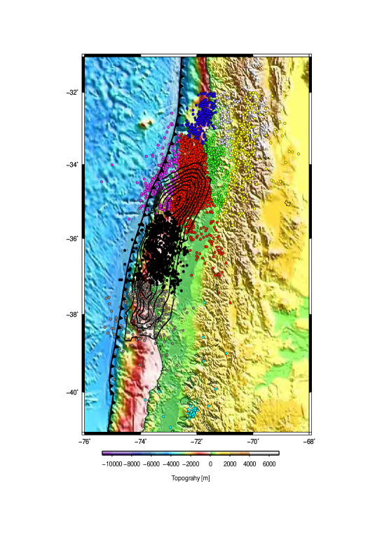
Figure 1: Map of the Chile region analyzed for slip and post-seismicity correlation with clustering events. The black-triangle line correspond to the trench.

In the second stage of our numerical work, we have introduced two variants. One was to consider only the areas were slip did take place in a non-negligible form, since our aim was exactly to examine the implications of the slip model. In addition, some numerical exploration has indicated that log-transformation of the quantities, slip and density function, lead to a more meaningful outcome. Since for a number of points the slip value is $0$, we adopted the modification commonly used in this case of adding a small positive quantity, that is working $\hbox{log}(k+\mathrm{slip})$, where $k$ is some small quantity. Since slip is measured in meters, then we adopted $k=0.01$ which represents a perturbation of only 1 cm of the original data. In the following, the term log-slip will be used for referring to $\hbox{log}(0.01+\mathrm{slip})$.

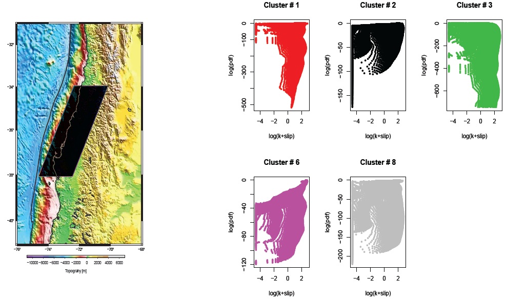
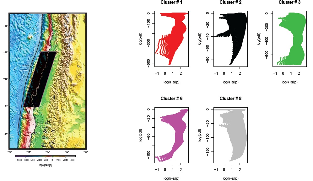
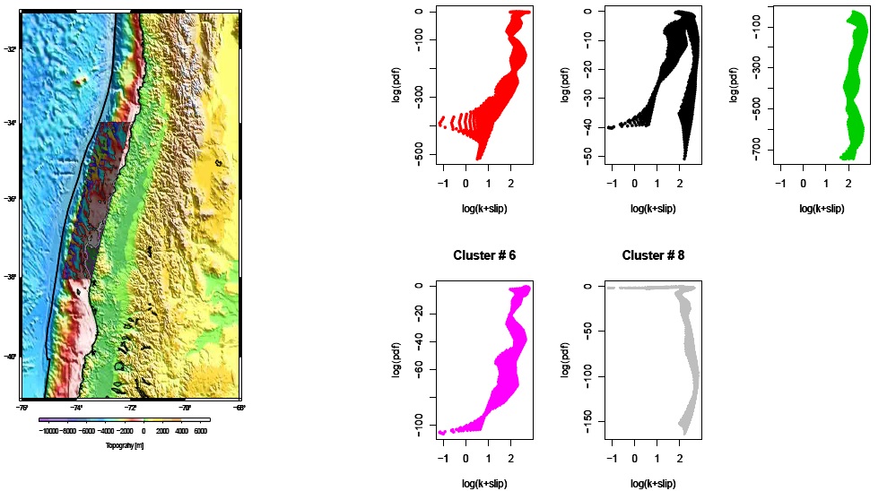
Figure 2: Left: Three grids considered for the NPC method (blacked shadows). Right: Relationship between log-slip and post-seismicity log-frequency for each grid. The points with $\mathrm{slip}=0$ produce verticals strips of points at abscissa $\hbox{log}(0.01)\approx-4.6$ in some of the top plots.

Furthermore, association between slip and events density can be examined in two different ways. One is to chose a regular grid of points in the region of interest, and evaluate these variables or their log-transforms over this grid. The other option is to evaluate these variables at the observed points of the seismic events.

Figure 2 refers to the first form, for three choices of the geographical area over which the grid of points is constructed. More precisely, the sets of points for which the computations have been performed have been obtained as the intersection of rectangular grids of sizes $(192\times 214)$, $(149\times\,214)$ and $(119\times\,214)$ with the three regions shown on the left side of Figure 2, of different geographical size. This process led then to consider three non-rectangular grids, comprising 19630, 10696 and 4812 points, respectively. The area covered by first grid includes the largest number of points associated of the seismic events of the data set, while the last one refers to the area with highest concentration of events. The right side of the figure displays the scatter plots of log-slip and log-density of the points, separately for each cluster. Only clusters labelled No. 1, 2, 3, 6, and 8 are considered here, since the other clusters of Figure 3 have been dropped, for the reason explained earlier.

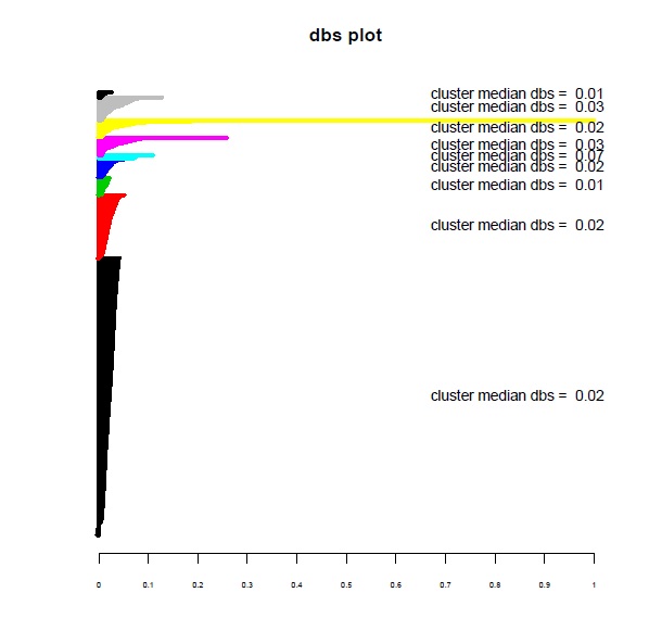
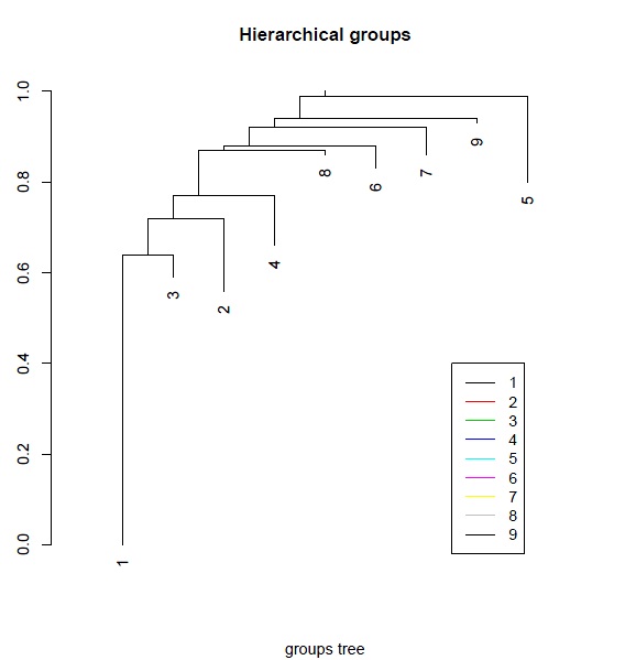
Figure 3: Plots of NPC method results.

Even if the selection of the three grids is somewhat subjective, the overall indication provided from Figure 2 provides convincing evidence of the presence association between the variables under consideration, specifically clusters labeled with No. 1, 2, and 6. This association is becoming more and more marked as we move down from the first to the last grid, that is when we focus on the area with greater intensity of events. The type of association is definitely non-linear, and so admittedly it does not lend itself to simple interpretation, but it is clearly present, especially so in the bottom portion of the figure.

Figure 4 refers instead to the second form of comparison, where evaluation of log-slip and log-density is performed at the observed location of events instead of a regular grid of points. Also this figure exhibits some noteworthy features. One is that in the red, black, violet, and grey clusters there exists a clear positive association between log-pdf and log-slip. Hence, the maximum slip is associated with high frequency of events. The green cluster does not display any association, presumably so because several events matching with null slip zone where probably have not been involved with the main earthquake; however the slip produced in this zone is lower. Pichilemu city ($34\mbox{.}38^{\circ}$S, $72\mbox{.}02^{\circ}$W) is located in the middle of the red cluster, approximately, which where the maximum slip is 16.6 meters. The sky-blue cluster correspond to seismic activity produced by Puyehue volcano eruption (June, 2011). Mocha Island ($38\mbox{.}39^{\circ}$S, $73\mbox{.}87^{\circ}$W) is located in the bottom of the gray cluster, which where the maximum slip is 11.9 meters (see Figure 1). In the black and gray clusters, we can see a positive association: the values of log-slip increments in the measure that the log-pdf increase.

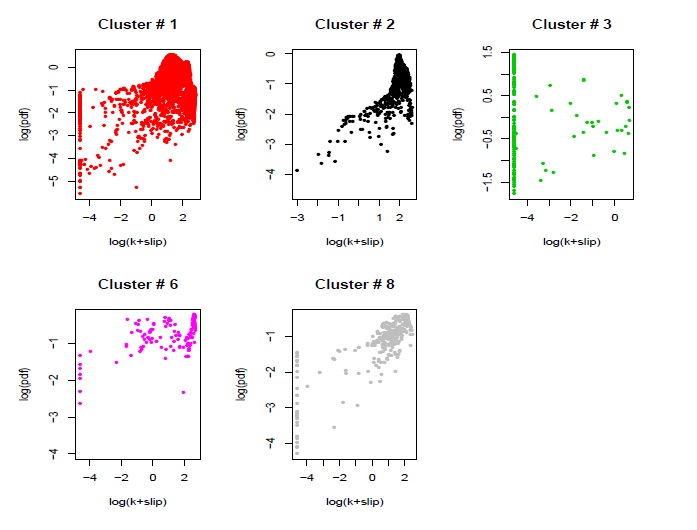
Figure 4: Relationship between log-slip and post-seismicity log-frequency for the clusters obtained for the NPC method of the first plot of Figure 3 that consider the slip model. The points with $\mathrm{slip}=0$ produce verticals strips of points at abscissa $\hbox{log}(0.01)\approx-4.6$

3.2 Nonparametric analysis of variance

A positive diagnostic of NPC allows us to implement the Kruskal-Wallis one-way analysis of variance method (KW; Kruskal & Wallis, 1952) by ranks that show the significance existence of slip between the clusters and consider a confidence level to testing what is the high slip of a cluster over the others. The KW is a classical method for testing whether samples originate from the same distribution where the null hypothesis is that the groups from which the samples originate, have the same median. Since it is a non-parametric method, the KW test does not assume a normal population or another distribution, but its purpose is analogous to the one of the classical analysis of variance for normal populations. The KW method consider a statistical test corrected by ties to compute the p-value and, large values of this test statistic produce the reject of the null hypothesis that the median of groups are equal. We made use of this method to test whether the clusters produced by the NPC method are associated to different slip measurements. The numerical outcome of the R function kruskal.test was $1861.5$ with an associated $p$-value (below $10^{-15}$), which provides an extreme indication of heterogeneity of slip among the clusters.

Table 2: $P$-values for Wilcoxon test for clusters slip.

	red	black	green	violet	gray
red	-	0	0	0.0181	0
black	0	-	0	0.3497	0
green	0	0	-	0	0
violet	0.0181	0.3497	0	-	0
gray	0	0	0	0	-

To examine where the differences among the groups are, we make use of the Wilcoxon test (Wilcoxon, 1945). This test perform individual test between two groups assuming for a null hypothesis that not exist differences between the two medians. The results are shown in Table 2. If each $p$-value is consider isolatedly, there is only on non-significant comparison at 5% level, but we must make an allowance for repeated testing; in this case, $10$ testing procedures have been performed. The more classical form of allowance for repeated testing is via the Bonferroni correction, which here leads to consider the $0.05/10=0.005$ significance level. Therefore, also the value $0.0181$ must be regarded as non-significant.

Table 3: Summary statistics of the slip variable by cluster and geodetic distance of clusters from the trench.

	Statistics					Geodetic Distance
Cluster	Mean	Min	Max	S.D.	N	Min	Max	Mean
red	6.200	0	16.566	4.329	4165	18.34	326.78	100.67
black	7.579	0.04	13.728	2.623	950	1.89	173.39	74.53
green	0.084	0	1.945	0.331	265	98.82	219.64	147.55
violet	7.572	0	15.043	5.752	149	1.31	168.93	27.56
gray	4.043	0	11.875	3.028	308	3.42	212.91	68.75

We can see in Table 3 that the red cluster representing the Pichilemu zone has the higher maximum of slip in relation with red (Constitución zone) and violet (Pichilemu’s offshore coast zone) clusters. With respect the gray (Arauco zone) and green (Rancagua city zone) clusters, present the lower values of slip and practically, the green cluster does not present slip.

The clustering estimation can be modified depending of the number of days after the mega earthquake and the observations involved in each day, so it may produce unequal results. Hence, for $t>1$, we compare the results at day $t$ respect to day $t-1$ to compare two alternative partitions of the same set. In each comparison it is necessary to keep the same number of clusters at day $t$ and $t+1$. Figure 5 shows the consistency of NP method along 200 days since the moment of the great earthquake with values higher than 0.89 for $HA$ case, 0.95 for $NSS$ and $HSS$ cases, and 0.7 for $HK$ case. In the first 200 days, some compressions between the clusters estimation at day $t$ versus day $t-1$ produce lower values of the indexes by the incorporation of one or more new groups related to the added observations.

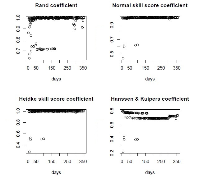
Figure 5: Plots of indexes of NPC results comparisons of data set at $t$ day versus $t-1$ day.

4 Discussion

The pronounced crustal aftershock activity with mainly normal faulting mechanisms is found in the Pichilemu region (Farías et al., 2011; Lange et al., 2012, Rietbrock et al., 2012). Lange et al., (2012) consider the processed events between 15 March and 30 September 2010 to estimate local magnitudes ($M_{l}$) in the Pichilemu region, where those magnitudes are comparable with the SSN magnitudes for large events. Specifically, a crustal aftershock activity is found in the region of Pichilemu ($\sim 34\mbox{.}5^{\circ}$S) where the crustal events occur in a $\sim 30$ km wide region with sharp inclined boundaries and oriented oblique to the trench. On the another hand, the aftershock seismicity parallel to the trench is apparent at 50-120 km distance perpendicular to the trench (see Table 3). Near $\sim 35^{\circ}$S and in the southern part of the rupture at $\sim 38^{\circ}$S occurs significant aftershock activity after the megathrust earthquake. This seismicity occurs in regions of high coseismic slip (see Table 3). Aftershocks and coseismic slip of the Maule 2012 earthquake terminate $\sim 50$ km south of the prolongation of the subducting Mocha Fracture zone around $\sim$($73\mbox{.}5^{\circ}$W, $38\mbox{.}5^{\circ}$S), near of the bottom of gray cluster (see Figure 1).

We have proposed an alternative way to clustering the aftershocks seismicity of the 2010 Maule earthquake $M_{W}$ 8.8. The nonparametric clustering has shown to be consistent in the measure that the dairy aftershocks events are added in the analysis and we present the diagnostic tools to illustrate this feature. We using a nonparametric kernel method to fit the high empirical aftershock frequency, which were highly correlated with the used coseismic slip model. Our findings can be explored further by considering an extended data set, including the events with delayed effect, and modeling the relationship of high coseismic slip areas and aftershock clusters. Also, this catalogue should be considered to the study of the behavior of a typical aftershock sequence, to identify outliers and to classify sequences into groups exhibiting similar aftershock behavior (Schoenberg & Tranbarger, 2008; Schoenberg et al., 2006). Finally, this analysis should be considered in the attempt to help identification of an increasing risk of occurrence of another great earthquake.

References

Azzalini, A., Torelli, N., 2007. Clustering via nonparametric density estimation. Stat. Comput. 17, 71-80.

Azzalini, A., Menardi, G., Rosolin, T., 2011. R package pdfCluster: Cluster analysis via nonparametric density estimation (version 0.1-13). URL http://cran.r-project.org/package=pdfCluster

Botev, Z.I., Grotowski, J.F., Kroese, D.P. (2010). Kernel Density Estimation Via Diffusion. Ann. Stat. 38, 5, 2916-2957.

Bowman, A.W., Azzalini, A., 1997. Applied Smoothing Techniques for Data Analysis: The Kernel Approach with S-Plus Illustrations. Oxford University Press, Oxford.

Brier, G.W., Allen, R.A., 1952. Verification of weather forecast. Compendium of Meteorology, Boston, Amer. Meteor. Soc., 841-848.

Contreras-Reyes, E., Carrizo, A., 2011. Control of high oceanic features and subduction channel on earthquake ruptures along the Chile-Perú subduction zone. Phys. Earth Planet. Inter. 186, 49-58.

Contreras-Reyes, J.E., Arellano-Valle, R.B., 2012. Kullback-Leibler divergence measure for Multivariate Skew-Normal Distributions. Entropy 14, 9, 1606-1626. doi:10.3390/e14091606.

Darwin, C., 1851. Geological Observations on Coral Reefs, Volcanic Islands and on South America. Londres, Smith, Elder and Co, pp. 768.

Dasgupta, A., Raftery, A.E., 1998. Detecting features in spatial point processes with cluster via model-based clustering. J. Amer. Statist. Assoc. 93, 294-302.

Delouis, B., Nocquet, J.M., Vallee, M., 2010. Slip distribution of the February 27, 2010 Mw = 8.8 Maule Earthquake, central Chile, from static and high-rate GPS, InSAR, and broadband teleseismic data. Geophys. Res. Lett. 37, L17305.

Farías, M., Comte, D., Roecker, S., Carrizo, D., Pardo, M., 2011. Crustal extensional faulting triggered by the 2010 Chilean earthquake: The Pichilemu Seismic Sequence. Tectonics 30, TC6010.

Hansen, A.W., Kuipers, W.H.A., 1965. On the relationship between the frequency of rain and various meteorological parameters. Koninklijke Nederlands Meteorologisch Institut, Meded. Verhand. 81, 2-15.

Hubert, L., Arabie, P., 1985. Comparing Partitions. J. Classif. 2, 193-218.

Kaufman, L., Rousseeuw, P.J., 1990. Finding Groups in Data: An Introduction to Cluster Analysis. New York: Wiley.

Kruskal, W., Wallis, W.A., 1952. Use of ranks in one-criterion variance analysis. J. Amer. Statist. Assoc. 47, 260, 583-621.

Lange, D., Tilmann, F., Barrientos, S., Contreras-Reyes, E., Methe, P., Moreno, M., Heit, B., Bernard, P., Vilotte, J., Beck, S., 2012. Aftershock seismicity of the 27 February 2010 Mw 8.8 Maule earthquake rupture zone. Earth Planet. Sci. Lett. 317-318, 413-425.

Lay, T., Ammon, C.J., Kanamori, H., Koper, K.D., Sufri, O., Hutko, A.R., 2010. Teleseismic inversion for rupture process of the 27 February 2010 Chile (Mw= 8.8) earthquake. Geophys. Res. Lett. 37, L13301.

Lorito, S., Romano, F., Atzori, S., Tong, X., Avallone, A., McCloskey, J., Cocco, M., Boschi, E., Piatanesi, A., 2011. Limited overlap between the seismic gap and coseismic slip of the great 2010 Chile earthquake. Nat. Geosci. 4, 173-177.

Menardi, G., 2010. Density-based silhouette diagnostics for clustering methods. Stat. Comput. 21, 295-308.

Moreno, M., Rosenau, M., Oncken, O., 2010. Maule earthquake slip correlates with pre-seismic locking of Andean subduction zone. Nature 467, 198-202.

Moreno, M., Melnick, D., Rosenau, M., Baez, J., Klotz, J., Oncken, O., Tassara, A., Chen, J., Bataille, K., Bevis, M., Socquet, A., Bolte, J., Vigny, C., Brooks, B., Ryder, I., Grund, V., Smalley, B., Carrizo, D., Bartsch, M., Hase, H., 2012. Toward understanding tectonic control on the Mw 8.8 2010 Maule Chile earthquake. Earth Planet. Sci. Lett., 321-322, 152-165.

Pollitz, F.F., Brooks, B., Tong, X., Bevis, M.G., Foster, J.H., B rgmann, R., Smalley, R.J., Vigny, C., Socquet, A., Ruegg, J.-C., Campos, J., Barrientos, S., Parra, H., Baez Soto, J.-C., Cimbaro, S., Blanco, M., 2011. Coseismic slip distribution of the February 27, 2010 Mw 8.8 Maule, Chile earthquake. Geophys. Res. Lett. 38, L09309.

R Development Core Team, 2012. R: A Language and Environment for Statistical Computing. R Foundation for Statistical Computing, Vienna, Austria. ISBN 3-900051-07-0, URL http://www.R-project.org.

Rietbrock, A., et al., 2012. Aftershock seismicity of the 2010 Maule Mw=8.8, Chile, earthquake: Correlation between co-seismic slip models and aftershock distribution? Geophys. Res. Lett. 39, L08310.

Rousseeuw, P.J., 1987. Silhouettes: A graphical aid to the interpretation and validation of cluster analysis. J. Comput. Appl. Math. 20, 53-65.

Ruegg, J., Rudloff, A., Vigny, C., Madariaga, R., de Chabalier, J.B., Campos, J., Kausel, E., Barrientos, S., Dimitrov, D., 2009. Interseismic strain accumulation measured by GPS in the seismic gap between Constitución and Concepción in Chile. Phys. Earth Planet. Inter. 175, 78-85.

Schoenberg, F.P., Brillinger, D.R., Guttorp, P., 2006. Point Processes, Spatial-Temporal. Encyclopedia of Environmetrics.

Schoenberg, F.P., Tranbarger, K.E., 2008. Description of earthquake aftershock sequences using prototype point patterns. Environmetrics 19, 271-286.

Vigny, C., Socquet, A., Peyrat, S., Ruegg, J.-C., M tois, M., Madariaga, R., Morvan, S., Lancieri, M., Lacassin, R., Campos, J., Carrizo, D., Bejar-Pizarro, M., Barrientos, S., Armijo, R., Aranda, C., Valderas-Bermejo, M.-C., Ortega, I., Bondoux, F., Baize, S., Lyon-Caen, H., Pavez, A., Vilotte, J.P., Bevis, M., Brooks, B., Smalley, R., Parra, H., Baez, J.-C., Blanco, M., Cimbaro, S., Kendrick, E., 2011. The 2010 Mw 8.8 Maule Mega-Thrust Earthquake of Central Chile, Monitored by GPS. Science 332 (6036), 1417-1421.

Wilcoxon, F., 1945. Individual comparisons by ranking methods. Biometrics 1, 80-83.

Zhu, Y., 2013. Nonparametric density estimation based on the truncated mean. Stat. Probabil. Lett. 83, 445-451.