A method for the reconstruction of unknown non-monotonic growth functions in the chemostat

Abstract

We propose an adaptive control law that allows one to identify unstable steady states of the open-loop system in the single-species chemostat model without the knowledge of the growth function. We then show how one can use this control law to trace out (reconstruct) the whole graph of the growth function. The process of tracing out the graph can be performed either continuously or step-wise. We present and compare both approaches. Even in the case of two species in competition, which is not directly accessible with our approach due to lack of controllability, feedback control improves identifiability of the non-dominant growth rate.

1 Introduction

We recall the classical chemostat model SW95 for a single species (biomass $b$) consuming a substrate (mass $s$):

$$\left\{\begin{array}[]{lll}\dot{s}&=&-\mu(s)b+D(s_{\mathrm{in}}-s)\\ \dot{b}&=&\mu(s)b-Db\end{array}\right.$$ (1)

where the dilution rate $D$ (the input) is the manipulated variable, which takes values in a bounded positive interval $[D_{\min},D_{\max}]$, and $\mu(\cdot)$ is a non-negative Lipschitz continuous function with $\mu(0)=0$ .

We consider here the following scenario: the function $\mu(\cdot)$ is unknown and possibly non-monotonic. Our objective is to reconstruct the graph of the function $\mu(\cdot)$ on the domain $(0,s_{\mathrm{in}})$ by varying the input $D$ in time. On-line measurements are only available for the variable $s$ (that is, $s$ is the output). This setup is realistic for experimental investigations such as in AHSA03 , however, demonstrations in this paper are based entirely on simulations of models such as system (1). The present paper analyzes and expands the ideas initially proposed by the authors in the conference paper SRRD12 .

Remark: Using model (1) tacitly assumes that the yield coefficient of the bio-conversion is known. This is why $\mu(s)b$ appears with the same pre-factor $1$ (once positive, and once negative) in both equations of (1) without loss of generality.

The problem of kinetics estimation in biological and biochemical models has been widely addressed in the literature (AW78 ; H82 ; HR82 ; R82 ; DB84 ; DB86 ; DP88 ; BD90 ; PM90 ; LF91 ; BSSR94 ; VK96 ; DP97 ; VCV97 ; KE98 ; VCV98 ; PFFD00 ; D03 ), either as a parameter estimation problem (one chooses a priori an analytical expression of the function $\mu(\cdot)$), or as an on-line estimation of the kinetics (one aims at determining $\mu(s(t))$ at the current time $t$). The theoretical identifiability of the graph of $\mu(\cdot)$ has been thoroughly studied in BG03 . In this paper, a practical method has been proposed to reconstruct the graph of $\mu(\cdot)$, based on a Kalman observer under the approximation that the function $z(t)=\mu(s(t))b(t)$ has a third time derivative equal to zero.

Here, we propose a different method that does not make any approximation of the dynamics. Our method exploits that it is sufficient to find the complete branch of equilibria of system (1) to identify the graph $\mu(\cdot)$. This reduces the system identification problem to a combination of two problems: finding the equilibria (a root-finding problem) and stabilizing them (a feedback control problem). Both of the latter two problems are in theory easily solvable with standard methods as we will explain and illustrate in Sections 2–5. The most difficult obstacle in practice is the implementation of a real-time feedback loop measuring $s$ and adapting $D$ with sufficient accuracy.

When the growth function is monotonic, a common way to reconstruct points on the graph of the growth function $\mu(\cdot)$ is to design a series of experiments fixing the dilution rate $D$ with different values and wait until the system settles to a steady state $(s^{\star},b^{\star})$ BD90 . As long as $D$ is less than $\mu(s_{\mathrm{in}})$, it is well known that the dynamics converges to a unique positive equilibrium that satisfies $\mu(s^{\star})=D$ (see for instance SW95 ). This technique requires the steady state to be stable in open loop, and consequently cannot reconstruct any part of the graph of a function $\mu(\cdot)$ where $\mu$ is non-increasing (such as the example shown schematically in Figure 1). Furthermore, the global convergence of this method is not satisfied in case of bi-stability, which is present in (1), with non-monotonic growth functions $\mu$ (see again SW95 ).

Figure 1: Domains of stability and instability in open-loop

An alternative approach is to fix a value of $s$, say $\bar{s}$, and design an adaptive control law $D(\cdot)$ that stabilizes the system about the steady state $(\bar{s},s_{\mathrm{in}}-\bar{s})$, with the value of $D$ converging to $\mu(\bar{s})$. Several adaptive control laws have been proposed in the literature for this problem. Nonlinear feedbacks require the knowledge of the growth function $\mu(\cdot)$, such as linearizing controls BD90 ; KH97 Extensions that are robust with respect to uncertainty on $\mu(\cdot)$ have been proposed RH02 but do not provide the precise reconstruction of $\mu(\bar{s})$. Several nonlinear PI based controllers, that do not require the precise knowledge of $\mu(\cdot)$, have been also proposed RC94 ; SC99 , but saturation and windup is often an issue (see JBV99 ; KD99 in similar frameworks). In AHSA03 , a dynamical output feedback has been proposed to globally stabilize such dynamics without the knowledge of $\mu(\cdot)$ and under the constraint $D\in[D_{\min},D_{\max}]$, but it requires the growth function to be monotonic. More recently, a saturated PI controller coupled with an observer, dedicated to the non-monotonic case, have been proposed to stabilize the dynamics about a nominal point that maximizes the biomass production SAL12 .

As the exploration of the unstable part of an unknown non-monotonic growth function requires an adaptive feedback, we propose in the present work to take advantage of an adaptation scheme for exploring (at least) a part of the graph instead of a limited number of set-points. We first consider that it can be useful to introduce a feedback control loop into (1) to identify the growth function $\mu$ of the open-loop system (1) (that is, (1) with constant input $D$). The feedback control law is initially a simple saturated proportionate controller:

$$D(s,\bar{D},\bar{s})=\mbox{sat}_{[D_{\min},D_{\max}]}\left(\bar{D}-G_{1}(s-\bar{s})\right)\mbox{,}$$ (2)

where $\bar{D}$ and $\bar{s}$ are reference values, and $G_{1}>0$ is the linear control gain. To ensure realistic values for the input $D$, feedback law (2) encloses the linear feedback rule into the saturation function

$$\mbox{sat}_{[D_{\min},D_{\max}]}(x)=\begin{cases}D_{\max}&\mbox{if $x>D_{\max}$,}\\ x&\mbox{if $x\in[D_{\min},D_{\max}]$,}\\ D_{\min}&\mbox{if $x<D_{\min}$,}\end{cases}$$

where the limits $D_{\min}$ and $D_{\max}$ are the extreme dilution rates that can be achieved experimentally. In sections 3 and 5 we will then explore adaptation rules for the reference values $(\bar{s},\bar{D})$ which ensure that asymptotically for $t\to\infty$ the input satisfies

$$D(s,\bar{D},\bar{s})=\bar{D}\,$$ (3)

or, equivalently, the output satisfies

$$s=\bar{s}\mbox{.}$$ (4)

If (4) is satisfied in the limit $t\to\infty$ then the controlled input $D$ in (2) equals the open-loop value $\bar{D}$ again (the feedback term $G_{1}(s-\bar{s})$ in (2) vanishes). We call feedback control that vanishes asymptotically non-invasive. The result is a new adaptive control law that stabilizes the dynamics about any desired equilibrium point without requiring a priori knowledge of its location, and whatever is the monotonicity of the growth function. One requirement on the adaptive law is that it should work uniformly well around a local maximum of $\mu$ (non-invasive feedback laws such as (wash-out) filtered feedback AWC94 or time-delayed feedback P92 do not achieve this).

We note that our adaptation rules will be much simpler than classical adaptive control laws BD90 ; AW94 . Usually, adaptive control aims to achieve a desired output regardless of changes in the underlying system. We only adapt the reference values to make the control input vanish and find branches of equilibria and bifurcations of the underlying system, similar to numerical continuation AG03 . While classical adaptive control requires system identification (an inverse problem) at some stage, our adaptation solves a root-finding problem, which is simpler.

Throughout our paper we assume that the output $s$ can be sampled and the input $D$ can be adjusted in quasi real-time. If the sampling period $T$ is not negligible, the approach presented here can still be applied. However, one then faces the problem that feedback stabilization of an unstable equilibrium at output $s$ becomes sensitive with amplification factor $\sim\exp(-\mu^{\prime}(s)T)$ to disturbances (note that $\mu^{\prime}(s)<0$ for unstable equilibria).

We show in Sections 4 and 5 that the feedback law (2) can be combined with an adaption rule for $(\bar{s},\bar{D})$ to reconstruct the graph of the growth function, even in the case of non-monotonic growth functions. Section 4 presents a dynamic adaption, whereas Section 5 introduces a step-wise adaptation. In Section 6 we investigate the case of two species that compete for the same common substrate.

2 Global stability of the simple feedback law (2)

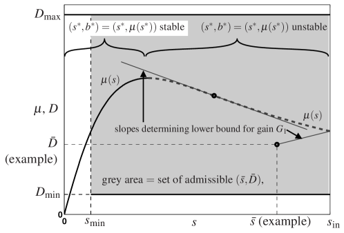
Figure 2: Sketch illustrating shape of growth function $\mu$ and set of admissible reference values

Let us first prove that the feedback law (2) is, within reasonable limits, globally stabilizing. Suppose that we choose the reference value $\bar{s}$ from an interval $[s_{\min},s_{\mathrm{in}})\subset(0,s_{\mathrm{in}})$, and that the limits on the input cover the growth function $\mu$ on this interval:

$$D_{\min} <\mu(s)\mbox{\quad for all $s\in[s_{\min},s_{\mathrm{in}}]$,}$$ (5)

$$D_{\max} >\mu(s)\mbox{\quad for all $s\in[0,s_{\mathrm{in}}]$.}$$ (6)

These conditions mean that the graph of $\mu$ does not cross the thick parts of the horizontal lines $D_{\min}$ and $D_{\max}$ bounding the grey area in Figure 2 from below and above.

Proposition 1

Suppose that the reference values $(\bar{s},\bar{D})$ in feedback law (2),

$$D(t)=\mbox{sat}_{[D_{\min},D_{\max}]}\left(\bar{D}-G_{1}(s(t)-\bar{s})\right)\mbox{,}$$

are chosen from the rectangle $[s_{\min},s_{\mathrm{in}})\times[D_{\min},D_{\max}]$, that the growth function $\mu$ satisfies (5)–(6), and that the gain $G_{1}$ is chosen sufficiently large, that is,

$$G_{1} >-\min_{s\in[0,s_{\mathrm{in}}]}\mu^{\prime}(s)\mbox{, and}$$ (7)

$$G_{1} >-\left[\frac{\mu(s_{\mathrm{in}})-\bar{D}}{s_{\mathrm{in}}-\bar{s}}\right]\mbox{.}$$ (8)

Then the controlled system (1) with $D=D(s,\bar{D},\bar{s})$ has a stable equilibrium $(s_{\mathrm{eq}},b_{\mathrm{eq}})\in[0,s_{\mathrm{in}})\times(0,\infty)$, which attracts all initial conditions $(s(0),b(0))\in[0,s_{\mathrm{in}})\times(0,\infty)$.

Proof

If $D>0$, and the growth function $\mu$ satisfies $\mu(0)=0$ and, for $s>0$, $\mu(s)>0$ then the set

$$R=\{(s,b):s\in[0,s_{\mathrm{in}}),b>0\}$$

is positively invariant (that is, trajectories starting in $R$ will stay in $R$ for all positive times). Furthermore, all trajectories starting in $R$ approach the subspace (called stochiometric set in SAL12 )

$$T=\{(s,b)\in R:s+b=s_{\mathrm{in}}\}$$

with rate at least $D_{\min}$ forward in time. This implies that it is sufficient to check if all trajectories in $T$ converge to a unique equilibrium. On $T$ the equation of motion can be expressed as a differential equation for $s$ only:

$$\dot{s}=[D(s,\bar{D},\bar{s})-\mu(s)][s_{\mathrm{in}}-s]=\left[\mbox{sat}_{[D_{\min},D_{\max}]}\left(\bar{D}-G_{1}(s-\bar{s})\right)-\mu(s)\right][s_{\mathrm{in}}-s]\mbox{.}$$ (9)

First, let us check that the equilibrium at $s=s_{\mathrm{in}}$ is unstable. The term $-G_{1}(s_{\mathrm{in}}-\bar{s})$ is negative such that $\bar{D}-G_{1}(s_{\mathrm{in}}-\bar{s})<D_{\max}$ for all admissible $\bar{D}$. Assumption (8) guarantees that $\bar{D}-G_{1}(s_{\mathrm{in}}-\bar{s})<\mu(s_{\mathrm{in}})$. Assumption (5) guarantees that also $D_{\min}<\mu(s_{\mathrm{in}})$. Hence,

$$D(s_{\mathrm{in}},\bar{D},\bar{s})-\mu(s_{\mathrm{in}})<0$$

for all admissible $(\bar{s},\bar{D})$. Thus, the prefactor of $s_{\mathrm{in}}-s$ in (9) is negative such that the equilibrium at $s_{\mathrm{in}}$ is unstable for all admissible $(\bar{s},\bar{D})$.

Since $\dot{s}>0$ at $s=0$, there must be other equilibria of (9) in $(0,s_{\mathrm{in}})$, which are given as solutions $s_{\mathrm{eq}}$ of $D(s_{\mathrm{eq}},\bar{D},\bar{s})=\mu(s_{\mathrm{eq}})$. Now let us check indirectly that none of the equilibria can satisfy $D_{\min}=\mu(s_{\mathrm{eq}})$.

Assume that (9) had an equilibrium $s_{\mathrm{eq}}$ with $D_{\min}=\mu(s_{\mathrm{eq}})$. Then $s_{\mathrm{eq}}$ has to be less than $s_{\min}$ due to assumption (5). However, if $s_{\mathrm{eq}}<s_{\min}$, then $\bar{D}-G_{1}(s_{\mathrm{eq}}-\bar{s})>\bar{D}\geq D_{\min}$ for all admissible $(\bar{s},\bar{D})$. Hence $D(s_{\mathrm{eq}},\bar{D},\bar{s})>D_{\min}$ (recall that $D_{\min}=\mu(s_{\mathrm{eq}})$ by assumption of the indirect proof) such that $D(s_{\mathrm{eq}},\bar{D},\bar{s})-\mu(s_{\mathrm{eq}})>0$, which means that $s_{\mathrm{eq}}$ cannot be equilibrium, establishing the contradiction.

Assumption (6) excludes that equilibria with $\mu(s_{\mathrm{eq}})=D_{\max}$ exist, hence all remaining equilibria $s_{\mathrm{eq}}\in(0,s_{\mathrm{in}})$ must satisfy

$$\bar{D}-G_{1}(s_{\mathrm{eq}}-\bar{s})=\mu(s_{\mathrm{eq}})\mbox{.}$$ (10)

Condition (7) ensures that this equation has a unique solution and that this solution corresponds to a stable equilibrium (which must be in $(0,s_{\mathrm{in}})$ because the boundaries of $(0,s_{\mathrm{in}})$ are inflowing for (9)).∎

Proposition 1 ensures that the output $s_{\mathrm{eq}}$ of the controlled system (1) with (2), after transients have decayed, is a well-defined smooth function of the parameters $(\bar{s},\bar{D})$ as long as $(\bar{s},\bar{D})$ are chosen from $(s_{\min},s_{\max})\times(D_{\min},D_{\max})$. We express this fact by using the bracket notation:

$$s_{\mathrm{eq}}(\bar{s},\bar{D})=\lim_{t\to\infty}s(t)\mbox{\quad where $s$ is output of \eqref{chemostat},\,\eqref{simple-feedback}.}$$ (11)

The function $s_{\mathrm{eq}}$ can be evaluated at any admissible point by setting the parameters $(\bar{s},\bar{D})$ in the definition (2) of the feedback rule, waiting until the transients of (1) have settled, and then reading off the output $s$. Equilibria of the uncontrolled system can then, according to (4), be found as roots of $s_{\mathrm{eq}}(\bar{s},\bar{D})-\bar{s}$. More specifically, we know that, for any admissible $\bar{s}$,

$$\bar{D}=\mu(\bar{s})\mbox{\quad if and only if $s_{\mathrm{eq}}(\bar{s},\bar{D})=\bar{s}$.}$$ (12)

Relation (12) permits us to identify $\mu(\bar{s})$ as the unique root of $s_{\mathrm{eq}}(\bar{s},\cdot)-\bar{s}$. Sections 3-5 will explore two strategies to find this root for a range of admissible $\bar{s}$ efficiently.

3 An adaptive control scheme

The first strategy is a dynamic feedback that comes on top of the feedback law (2) for $D$. We treat $\bar{D}$ not as a parameter but introduce an additional dynamical equation for $\bar{D}$, achieving local convergence of the output $s$ to any reference value $\bar{s}\in(0,s_{\mathrm{in}})$ without the knowledge of the growth function $\mu$. Then the asymptotic value of $\bar{D}$ allows one to reconstruct the value $\mu(\bar{s})$.

Proposition 2

Fix a number $\bar{s}\in(0,s_{\mathrm{in}})$ and take numbers $D_{\min}$, $D_{\max}$ that fulfill $0<D_{\min}<\mu(\bar{s})<D_{\max}$. Then the dynamical feedback law

$$\begin{split}D(s,\bar{D})&=\mbox{sat}_{[D_{\min},D_{\max}]}\left(\bar{D}-G_{1}(s-\bar{s})\right)\\ \frac{\mathop{}\!\mathrm{d}}{\mathop{}\!\mathrm{d}t}\bar{D}&=-G_{2}(s-\bar{s})(\bar{D}-D_{\min})(D_{\max}-\bar{D})\end{split}$$ (13)

exponentially stabilizes the system (1) locally about $(s,b)=(\bar{s},s_{\mathrm{in}}-\bar{s})$, for any positive constants $(G_{1},G_{2})$ such that $G_{1}>-\mu^{\prime}(\bar{s})$. Furthermore one has

$$\lim_{t\to+\infty}\bar{D}(t)=\mu(\bar{s})$$

Remark. Our adaptive control is in this case similar to a classical PI controller. The quantity $\bar{D}$ is playing the role of the I part, but staying bounded by construction. It is also similar to gain-scheduling methods but here the parameter $\bar{D}$ is evolving continuously, as a state variable.

Proof

Locally about $s=\bar{s}$, the closed loop system is equivalent to the three-dimensional dynamical system

$$\begin{cases}\begin{aligned} \frac{\mathop{}\!\mathrm{d}}{\mathop{}\!\mathrm{d}t}s\ &=-\mu(s)b+(\bar{D}-G_{1}(s-\bar{s}))(s_{\mathrm{in}}-s)\\ \frac{\mathop{}\!\mathrm{d}}{\mathop{}\!\mathrm{d}t}b\ &=\phantom{-}\mu(s)b-(\bar{D}-G_{1}(s-\bar{s}))b\\ \frac{\mathop{}\!\mathrm{d}}{\mathop{}\!\mathrm{d}t}\bar{D}&=-G_{2}(s-\bar{s})(\bar{D}-D_{\min})(D_{\max}-\bar{D})\end{aligned}\end{cases}$$

This system admits the unique positive equilibrium $E^{\star}=(\bar{s},s_{\mathrm{in}}-\bar{s},\mu(\bar{s}))$.
For simplicity, we write the dynamics in the variables $(z,s,\bar{D})$ coordinates, where $z$ is defined as $z=s+b$:

$$\begin{cases}\begin{aligned} \frac{\mathop{}\!\mathrm{d}}{\mathop{}\!\mathrm{d}t}z\ &=(\bar{D}-G_{1}(s-\bar{s}))(s_{\mathrm{in}}-z)\\ \frac{\mathop{}\!\mathrm{d}}{\mathop{}\!\mathrm{d}t}s\ &=-\mu(s)(z-s)+(\bar{D}-G_{1}(s-\bar{s}))(s_{\mathrm{in}}-s)\\ \frac{\mathop{}\!\mathrm{d}}{\mathop{}\!\mathrm{d}t}\bar{D}&=-G_{2}(s-\bar{s})(\bar{D}-D_{\min})(D_{\max}-\bar{D})\end{aligned}\end{cases}$$

The Jacobian matrix at $E^{\star}$ in these coordinates is

$$\left(\begin{array}[]{ccc}-\mu(\bar{s})&0&0\\ -\mu(\bar{s})&-(\mu^{\prime}(\bar{s})+G_{1})(s_{\mathrm{in}}-\bar{s})&s_{\mathrm{in}}-\bar{s}\\ 0&-G_{2}(\mu(\bar{s})-D_{\min})(D_{\max}-\mu(\bar{s}))&0\end{array}\right)$$

Its eigenvalues are $\lambda_{1}=-\mu(\bar{s})<0$ and $\lambda_{2}$, $\lambda_{3}$ as eigenvalues of the sub-matrix

$$M=\left(\begin{array}[]{cc}-(\mu^{\prime}(\bar{s})+G_{1})(s_{\mathrm{in}}-\bar{s})&s_{\mathrm{in}}-\bar{s}\\ -G_{2}(\mu(\bar{s})-D_{\min})(D_{\max}-\mu(\bar{s}))&0\end{array}\right)$$

Then, one has

$$\begin{array}[]{lll}\mbox{det}(M)&=&G_{2}(\mu(\bar{s})-D_{\min})(D_{\max}-\mu(\bar{s}))(s_{\mathrm{in}}-\bar{s})\\ \mbox{tr}(M)&=&-(\mu^{\prime}(\bar{s})+G_{1})(s_{\mathrm{in}}-\bar{s})\end{array}$$

and concludes about the exponential stability of $E^{\star}$ when $G_{2}>0$ and $G_{1}>-\mu^{\prime}(\bar{s})$. Finally, one obtains from (13) that $D$ or $\bar{D}$ converges toward the unknown value $\mu(\bar{s})$.∎

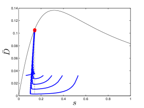
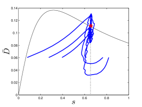
Figure 3: The behavior of feedback law (13) for two different values of $\bar{s}$ in the $(s,\bar{D})$-projection. Parameters: $G_{1}=2$, $G_{2}=2$, output disturbance defined in (15).

Note that the assumptions in Proposition 2 (for example, on the gain $G_{1}$) are weaker than those of Proposition 1 as Proposition 2 is only concerned with local stability and a single reference value $\bar{s}$.

Figure 3 demonstrates how control law (13) stabilizes an equilibrium with output $\bar{s}$ for $\bar{s}$ in the increasing (left panel) and decreasing (right panel) part of the growth law $\mu$. For our single-species demonstration we choose the non-monotonic Haldane function

$$\mu(s)=\frac{s}{1+s+10s^{2}}$$ (14)

and $s_{\mathrm{in}}=1$. Any other growth function could have been chosen, under the requirements that it is Lipschitz continuous and fulfill equations (5) and (6). To illustrate the effect of disturbances, we super-impose a rapid oscillation onto the measurements of output $s$, such that the output has the form

$$s_{\mathrm{output}}=s[1+\delta\cos(3t)\sin(t)]\mbox{,\quad where\quad}\delta=0.05$$ (15)

(other disturbances such as quasi-periodic or white-noise signals have been tested, getting similar results). The grey background curve in Figure 3 shows $\mu(\cdot)$, which is clearly non-monotonic on the domain $(0,s_{\mathrm{in}})$ ($s_{\mathrm{in}}=1$). To show the robustness of the method, we we have chosen $\bar{D}(0)$ slightly far from $\mu(s(0))$.

4 Reconstruction of the growth function

Now, we can trace out any desired part of the graph $\mu(\cdot)$ dynamically by letting $\bar{s}$ change slowly with time as solution of the simple dynamics

$$\frac{\mathop{}\!\mathrm{d}}{\mathop{}\!\mathrm{d}t}\bar{s}=\varepsilon\bar{s}(s_{\mathrm{in}}-\bar{s})$$ (16)

to explore the right part of the graph of $\mu(\cdot)$ when $\varepsilon$ is a small non-negative number, and to explore the left one when $\varepsilon$ is a small non-positive number. During the reconstruction of the graph, the gain $G_{1}$ has to be been chosen uniformly large according to (7). Figure 4 shows how the adaptation rule (16) together with (13) reconstructs the entire graph of the growth function. The overall time it took to reach $\bar{s}=0.9$ is $t\approx 3000$ in the dimensionless time units of (1).

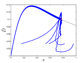
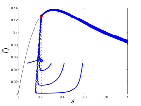
Figure 4: Dynamical adaptation using (16) to explore dynamically the left and right part of the graph of the unknown function $\mu(\cdot)$. Parameters: for the left panel, $\varepsilon=+0.001$, for the right panel, $\varepsilon=-0.001$, otherwise identical to Fig. 3.

5 Step-wise adaptation of the reference values

In this section, we propose an alternative to the continuous adaptation of $\bar{D}$ and $\bar{s}$: we treat the root problem $0=s_{\mathrm{eq}}(\bar{s},\bar{D})-\bar{s}$ with ordinary numerical root-finders such as the Newton iteration. We present here an approach that combines the two steps of the method (the adaptive control and the continuation) in a step-wise framework.

5.1 Adaptation using Newton iteration

In an experimental setting one will have to adapt the numerical methods to the lower accuracy of experimental outputs (see SGNWK08 for a demonstration in a mechanical experiment) but for this paper we restrict ourselves to a numerical demonstration. In the single-species chemostat one profits from the knowledge of an approximate derivative of $s_{\mathrm{eq}}$ with respect to $\bar{D}$, making the Newton iteration more efficient. Suppose, we plan to identify the growth function $\mu$ in a sequence of points $\bar{s}_{k}=\bar{s}_{0}+k\delta$ (where $\delta>0$ is small). The function values $\mu(\bar{s}_{k})$ are the roots $\bar{D}_{k}$ of $s_{\mathrm{eq}}(\bar{s}_{k},\cdot)-\bar{s}_{k}$, where $s_{\mathrm{eq}}(\bar{s},\bar{D})$ was the asymptotic output of the chemostat (1) with simple feedback control (2), as defined by (11). The equilibrium value $s_{\mathrm{eq}}(\bar{s},\bar{D})$ satisfies $\mu(s_{\mathrm{eq}}(\bar{s},\bar{D}))=D-G_{1}(s_{\mathrm{eq}}(\bar{s},\bar{D})-\bar{s})$ due to (1) (see also (10)) for all admissible $\bar{D}$. Differentiating this implicit expression with respect to $\bar{D}$, we obtain

$$\frac{\partial s_{\mathrm{eq}}}{\partial\bar{D}}(\bar{D},\bar{s}_{k})=\frac{1}{G_{1}+\mu^{\prime}(s_{\mathrm{eq}}(\bar{D},\bar{s}_{k}))}\approx\frac{1}{G_{1}+\frac{\bar{D}-\bar{D}_{k-1}}{\bar{s}_{k}-\bar{s}_{k-1}}}\mbox{,}$$

where we used a secant approximation for $\mu^{\prime}$ on the right-hand side. This leads to the iteration rule

$$\bar{D}_{\mathrm{new}}=\bar{D}_{\mathrm{old}}-\frac{s_{\mathrm{eq}}(\bar{D}_{\mathrm{old}},\bar{s}_{k})}{G_{1}+\frac{\bar{D}_{\mathrm{old}}-\bar{D}_{k-1}}{\bar{s}_{k}-\bar{s}_{k-1}}}\mbox{,}$$ (17)

starting from $\bar{D}=\bar{D}_{k-1}$, or (for $k>2$)

$$\bar{D}=\bar{D}_{k-1}+\frac{\bar{D}_{k-1}-\bar{D}_{k-2}}{\bar{s}_{k-1}-\bar{s}_{k-2}}\mbox{.}$$

For the initial step ($k=1$) the derivative of $s_{\mathrm{eq}}$ has to be either guessed or approximated with a finite difference (we used the latter in our numerical simulations).

Note that at no point it is necessary to set the internal states $s$ or $b$ of system (1). Only the reference values $(\bar{s},\bar{D})$ have to be set.

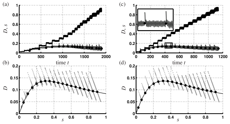
Figure 5: Simulation of step-wise adaptation. Panels (a) and (b) use (17) where $\bar{s}_{k}=0.05k$. Panels (c) and (d) use (18)–(19) where $\delta=0.05$, both cases subject to output disturbance (15). Parameters: $\mathtt{tol}=10^{-3}$ (for (a) and (b)), $G_{1}=1$, $D_{\max}=0.2$, $D_{\min}=0.02$. A check if the transients have settled was performed every $20$ time units. Transients were accepted as settled if the standard deviation of $s$ ($\operatorname{std}(s)$) on the last interval is no longer smaller than $0.9\operatorname{std}(s)$ on the previous interval. The average over the last interval is used as the resulting equilibrium.

The panels (a) and (b) of Figure 5 show the output of a simulation with the step-wise adaptation using Newton iteration (17). Panels (a) shows the time profile of output $s$ and input $D$ throughout the run. Panels (b) shows the evolution in the $(s,D)$-plane in grey. Black dots indicate when convergence was reached ($|s_{\mathrm{eq}}-\bar{s}_{k}|<\mathtt{tol}$. These points correspond to values at which the control was accepted as non-invasive. Then the iteration moved on to the next $\bar{s}_{k}$. By gradually tracing out the graph of $\mu$, one achieves small and rapidly decaying transients in every evaluation of $s_{\mathrm{eq}}$ (which involves running system (1) with control until transients have settled). This is so because the transients all lie inside the subspace $\{(s,b):s+b=s_{\mathrm{in}}\}$ after system (1) has run at least once. Second, the initial offset from the equilibrium is always small, because the adjustments of $\bar{s}$ and $\bar{D}$ are small.

5.2 A simplified step-wise scheme

The scheme (17) permits one to find $\mu(\bar{s}_{k})$ for an a priori prescribed set of admissible abscissae $\bar{s}_{k}$. If one wants to recover only the graph of $\mu$ one does not need to prescribe the sequence $\bar{s}_{k}$ a priori, thus, avoiding a Newton iteration. Suppose that we know already two points $p_{k-1}=(\bar{s}_{k-1},\bar{D}_{k-1})$ and $p_{k}=(\bar{s}_{k},\bar{D}_{k})$ on the curve $(s,\mu(s))$. Then we set

$$(\bar{s}_{\mathrm{pred},k+1},\bar{D}_{\mathrm{pred},k+1})=p_{k}+\delta\frac{p_{k}-p_{k-1}}{\|p_{k}-p_{k-1}\|}\mbox{,}$$ (18)

where $\delta>0$ is the approximate desired distance between points along the curve $(s,\mu(s))$, and run the controlled experiment with the reference values $(\bar{s},\bar{D})=(\bar{s}_{\mathrm{pred},k+1},\bar{D}_{\mathrm{pred},k+1})$ in (2) until the transients have settled to obtain the next point on the curve

$$\begin{split}\bar{s}_{k+1}&=s_{\mathrm{eq}}(\bar{s}_{\mathrm{pred},k+1},\bar{D}_{\mathrm{pred},k+1})\\ \bar{D}_{k+1}&=D(\bar{s}_{k+1},\bar{D}_{\mathrm{pred},k+1},\bar{s}_{\mathrm{pred},k+1})\\ &=\bar{D}_{\mathrm{pred},k+1}-G_{1}(\bar{s}_{k+1}-\bar{s}_{\mathrm{pred},k+1})\end{split}$$ (19)

This simplified procedure cannot guarantee the identification of $\mu$ at prescribed equidistantly spaced values of $s$ but finds $\mu(\bar{s}_{k})$ for a (nearly evenly spaced) sequence $\bar{s}_{k}$ given by the intersections of the lines $D=D_{\mathrm{pred},k}-G_{1}(s-\bar{s}_{\mathrm{pred},k})$ with the graph $D=\mu(s)$.

Figure 5, panels (c) and (d), demonstrate the speed-up using the simplified scheme (18)–(19) (note the times at the abscissae). The difference to Figure 5(a,b) is that the values $\bar{s}_{k}$ at which the growth function is evaluated are not exactly equidistantly spaced. The zoom in Figure 5(c) shows that the control reaches the equilibrium up to an error at the level of the disturbance very quickly. The black dot shows then the average of the output during the remainder of the time before the output gets accepted (thus, achieving higher accuracy at the cost of speed).

6 The two species case

Let us now consider an extension of the chemostat model (1) that considers two species which compete for the same substrate. The two-species model can be written as follows

$$\left\{\begin{array}[]{lll}\dot{s}&=&\displaystyle-\sum_{i=1}^{2}\mu_{i}(s)b_{i}+D(s_{\mathrm{in}}-s)\\[8.53581pt] \dot{b}_{i}&=&\mu_{i}(s)b_{i}-Db_{i}\qquad(i=1,2)\end{array}\right.$$ (20)

The two-species model has co-existing equilibria $E^{*}_{i}$, which correspond to the state where species $i$ is present and the other species $3-i$ is suppressed. The following proposition shows first that feedback stabilization based on input $D$ and output $s$ breaks down in general for the equilibrium corresponding to the species with the smaller growth rate (the suppressed, or non-dominant, species). Then we state what eigenvalues the linearizations at equilibria have for our specific control laws, (2) and (13).

Proposition 3

Fix $\bar{s}\in(0,s_{\mathrm{in}})$ and consider the equilibrium $E_{2}^{\star}=(\bar{s},0,s_{\mathrm{in}}-\bar{s})$.

1. (Suppressed equilibrium not stabilizable) Let $\mu_{1}(\bar{s})>\mu_{2}(\bar{s})$, and $D(\cdot)$ be a feedback $D(\cdot)$ of the form

   $$D=f(s,\xi)\mbox{,}\quad\dot{\xi}=g(s,\xi)\mbox{, \qquad( $\xi\in\mathbb{R}^{k}$)}$$ (21)

   with $f(\bar{s},0)=\mu_{2}(\bar{s})$ and $g(\bar{s},0)=0$. Then the equilibrium $E_{2}^{\star}$ of system (20) with feedback $D$ is unstable.

2. (Eigenvalues for simple feedback) Using feedback law (2),

   $$D(s,\bar{D},\bar{s})=\mbox{sat}_{[D_{\min},D_{\max}]}\left(\bar{D}-G_{1}(s-\bar{s})\right)$$

   with $D_{\min}$ and $D_{\max}$ such that $D_{\min}<\mu_{2}(\bar{s})<D_{\max}$, the linearization of system (1) in the equilibrium $E_{2}^{\star}$ has the eigenvalues $-\mu_{2}(\bar{s})$, $\mu_{1}(\bar{s})-\mu_{2}(\bar{s})$ and $-(\mu^{\prime}_{2}(\bar{s})+G_{1})(s_{\mathrm{in}}-\bar{s})$.

3. (Dominant equilibrium stabilized by dynamic feedback) If $\mu_{1}(\bar{s})<\mu_{2}(\bar{s})$, then the feedback (13) exponentially stabilizes the system (20) locally about $E_{2}^{\star}$, for any positive constants $(G_{1},G_{2})$ such that $G_{1}>-\mu_{2}^{\prime}(\bar{s})$. Furthermore one has

   $$\lim_{t\to+\infty}\bar{D}(t)=\mu_{2}(\bar{s})$$

Proof

Consider the dynamics of the two-species model (20) with feedback $D$ given by (21)

$$\left\{\begin{array}[]{lll}\dot{s}&=&\displaystyle-\sum_{i=1}^{2}\mu_{i}(s)b_{i}+f(s,\xi)(s_{\mathrm{in}}-s)\\[11.38109pt] \dot{b}_{i}&=&\mu_{i}(s)b_{i}-f(s,\xi)b_{i}\qquad(i=1,2)\\ \dot{\xi}&=&g(s,\xi)\mbox{.}\end{array}\right.$$

We write this system in $(z,b_{1},b_{2},\xi)$ coordinates with $z=s+b_{1}+b_{2}$:

$$\left\{\begin{array}[]{lll}\dot{z}&=&f(z-b_{1}-b_{2},\xi)(s_{\mathrm{in}}-z)\\ \dot{b}_{i}&=&(\mu_{i}(z-b_{1}-b_{2})-f(z-b_{1}-b_{2},\xi))b_{i}\\ \dot{\xi}&=&g(z-b_{1}-b_{2},\xi)\mbox{.}\end{array}\right.$$

Point 1: at equilibrium $E_{2}^{\star}$, the Jacobian matrix $J_{2}^{\star}$ possesses the following form in $(z,b_{1},b_{2},\xi)$ coordinates

$$J_{2}^{\star}=\left(\begin{array}[]{cccc}-\mu_{2}(\bar{s})&0&0&0\\ 0&\mu_{1}(\bar{s})-\mu_{2}(\bar{s})&0&0\\ \star&\star&\star&\star\\ \star&\star&\star&\star\end{array}\right)\mbox{,}$$ (22)

which has the positive eigenvalue $\mu_{1}(\bar{s})-\mu_{2}(\bar{s})$. This proves that $E^{*}_{2}$ is unstable whatever the choice of the feedback $D(\cdot)$.

Point 2: we can be more specific about the form of $J_{2}^{\star}$ for the simple feedback law (2). Since $D_{\min}<\mu_{2}(\bar{s})<D_{\max}$, the feedback is in its linear regime, such that $\partial_{s}D=-G_{1}$. Thus, (component $\xi$ is absent)

$$J_{2}^{\star}=\begin{pmatrix}-\mu_{2}(\bar{s})&0&0\\ 0&\mu_{1}(\bar{s})-\mu_{2}(\bar{s})&0\\ \star&\star&-(\mu^{\prime}_{2}(\bar{s})+G_{1})(s_{\mathrm{in}}-\bar{s})\end{pmatrix}$$

Point 3: for feedback law (13) $J_{2}^{\star}$ can be written as follows, in $(z,b_{1},b_{2},\bar{D})$ coordinates

$$J_{2}^{\star}=\begin{pmatrix}\begin{matrix}-\mu_{2}(\bar{s})&0\\ 0&\mu_{1}(\bar{s})-\mu_{2}(\bar{s})\\ \star&\star\end{matrix}\quad&\begin{matrix}\begin{matrix}0&0\\ 0&0\end{matrix}\\ M\end{matrix}\end{pmatrix}\mbox{,}$$

where $M$ is a $2\times 2$ matrix with the entries

$$M=\begin{pmatrix}-(\mu_{2}^{\prime}(\bar{s})+G_{1})(s_{\mathrm{in}}-\bar{s})&\quad&s_{\mathrm{in}}-\bar{s}\\ -G_{2}(\mu_{2}(\bar{s})-D_{\min})(D_{\max}-\mu_{2}(\bar{s}))&\quad&0\end{pmatrix}$$

Its eigenvalues are $\lambda_{1}=-\mu_{2}(\bar{s})<0$, $\lambda_{2}=\mu_{1}(\bar{s})-\mu_{2}(\bar{s})<0$, $\lambda_{3}$ and $\lambda_{4}$ with

$$\begin{array}[]{lll}\lambda_{3}\lambda_{4}&=&G_{2}(\mu_{2}(\bar{s})-D_{\min})(D_{\max}-\mu_{2}(\bar{s}))(s_{\mathrm{in}}-\bar{s})\\ \lambda_{3}+\lambda_{4}&=&-(\mu_{2}^{\prime}(\bar{s})+G_{1})(s_{\mathrm{in}}-\bar{s})\end{array}$$

As in the proof of Proposition 2, one concludes the exponential stability of $E^{\star}_{2}$ when $G_{2}>0$ and $G_{1}>-\mu_{2}^{\prime}(\bar{s})$, and the convergence of $D(\cdot)$ toward $\mu_{2}(\bar{s})$.∎

Consequently, the adaptive control scheme proposed in Section 3 only allows one to reconstruct the larger of the two growth rates at any given $s$ by stabilizing the equilibrium.

Nevertheless, the introduction of feedback control may still be of help. To be specific, let us assume that species $1$ is dominant for $s<s_{c}$ (and species $2$ is suppressed there), and species $2$ is dominant for $s>s_{c}$, where $s_{c}$ is a cross-over point: $\mu_{1}(s)>\mu_{2}(s)$ for $s<s_{c}$ and $\mu_{1}(s)<\mu_{2}(s)$ for $s>s_{c}$ (see the underlying function graphs in Figure 6 for a typical picture of the discussed scenario, $s_{c}=0.5$ in Fig. 6). Suppose we are interested in the location of $E_{2}^{\star}$ to identify $\mu_{2}(\bar{s})$ for $\bar{s}<s_{c}$. As the form of the Jacobian $J_{2}^{\star}$ in (22) makes clear, two eigenvalues of $J_{2}^{*}$ are unaffected by our feedback control. One of them, $-\mu_{2}(\bar{s})$ is always stable. It corresponds to the transversally stable direction of the invariant subspace $T=\{(s,b_{1},b_{2}):s+b_{1}+b_{2}=s_{\mathrm{in}}\}$. Once, the system is in $T$, control will not move it out of $T$, thus, we can ignore this eigenvalue.

The other uncontrollable eigenvalue, $\mu_{1}(\bar{s})-\mu_{2}(\bar{s})$, is unstable for $\bar{s}<s_{c}$, but stable for $\bar{s}>s_{c}$. Consequently, the following strategy would make it possible in principle to identify $\mu_{2}$ for $\bar{s}<s_{c}$: keep the system in the region where $s>s_{c}$ for some time to suppress species $1$ (which will exponentially decay for $s>s_{c}$ according to Proposition 3, point 2). When one is sufficiently close to the invariant line $L_{2}=\{(s,b_{1},b_{2}):b_{1}=0,s+b_{2}=s_{\mathrm{in}}\}$, one is (nearly) in the single-species case, where one can then use the methods of Sections 3, 4 or 5 to explore $\mu_{2}$ for a finite time for $s<s_{c}$ until species $1$ has recovered. This approach is also possible without control if both growth functions are monotone.

Figure 6(b) demonstrates the application of feedback law (13) in combination with (16), which defines the adaptive control presented in Section 4, to the two-species situation with the monotonic Monod functions

$$\mu_{1}(s)=\frac{s}{0.1+s},\qquad\mu_{2}(s)=1.5\frac{s}{0.4+s}$$ (23)

as growth rates.

If one treats $\bar{s}$ as a parameter then the equilibria $E^{*}_{1}$ and $E^{*}_{2}$ undergo an exchange of stability (a degenerate transcritical bifurcation) at $\bar{s}=s_{c}$. As the adaptation rule (16) lets $\bar{s}$ drift slowly (with speed $\varepsilon$) the full system exhibits a phenomenon known as delayed loss of stability BS99 ; LRS09 in the context of dynamic bifurcations B91 , widely studied in slow-fast systems O91 . Say, we are decreasing $\bar{s}$ slowly from above $s_{c}$ to below $s_{c}$ (as in Figure 6(a)). Then concentration $b_{1}$ decreases exponentially, coming close to $0$ while $\bar{s}>s_{c}$. After $\bar{s}$ has crossed $s_{c}$, the concentration $b_{1}$ grows exponentially, but still takes some time until it reaches values noticeably different from $0$. The value $\bar{s}_{\mathrm{loss}}$ of $\bar{s}$ at which $b_{1}$ becomes noticeably non-zero is in the ideal ODE model independent of the drift speed $\varepsilon$ of $\bar{s}$. Figure 6(a) shows this effect: since $b_{1}$ is nearly zero the variable $D$ continues to follow the, by now unstable, drifting equilibrium $E^{*}_{2}$. For a given $\bar{s}>s_{c}$ and an arbitrary small $b_{1\mathrm{ini}}>0$ at time $0$, the value $\bar{s}_{\mathrm{loss}}<s_{c}$ at which $b_{1}$ reaches $b_{1,\mathrm{ini}}$ again when following (16), is given implicitly by the relation

$$\int_{\bar{s}}^{\bar{s}_{\mathrm{loss}}}(\mu_{1}(\sigma)-\mu_{2}(\sigma))/(\sigma(s_{in}-\sigma))d\sigma=0$$

in the limit of small $\epsilon$. This delay mechanism allows one in principle a reconstruction of a part of the smaller growth rate close to the bifurcation value of $\bar{s}$.

Remark 1: From a practical view point, an apparent jump between the two graphs (see evolution curves in black in Fig. 6) could indicate the presence of another species, if one believes that the culture in chemostat was initially pure. Nevertheless, one can still rely on the reconstruction of parts of growth curves for each species.

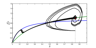
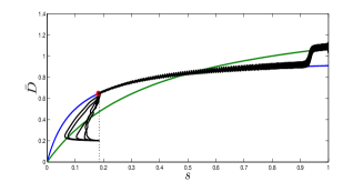
Figure 6: Exploiting the delayed loss of stability for the dynamic control feedback law (13) in the two species case with growth rates given in (23) (shown underlying in both panels). The reference value $\bar{s}$ is decreasing on the left panel, and increasing on the right one. Parameters: $\epsilon=-0.01$ for panel (a) and $\epsilon=0.01$ for panel (b) in (16), $G_{1}=2$, $G_{2}=2$ in (13), output disturbance defined in (15).

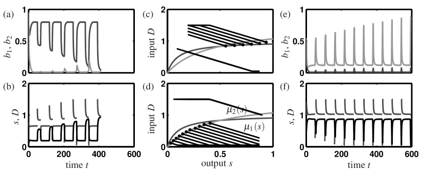
Figure 7: Jumping back and forth between two regions at discrete times exploiting the delayed loss of stability for the simple control feedback law (2) in the two species case with growth rates given in (23) (shown underlying in both panels (c) and (d)).

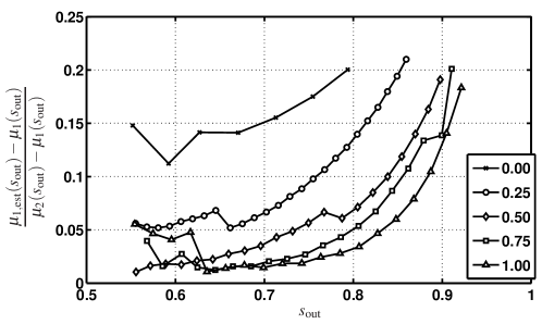
Figure 8: Effect of feedback control (2) on accuracy of identified growth rate $\mu_{2}$. Parameters are the same as for Figure 7(a-c) (in particular, $b_{\min}=10^{-3}$), the gain $G_{1}$ is shown in the legend. Parameters: $G_{1}=1$, $D_{\max}=1.5$, $D_{\min}=0.1$ in (2), $b_{\min}=10^{-3}$, output disturbance defined in (15).

Remark 2: In the idealized ODE model one could in principle recover the entire suppressed part of the growth rate by spending more time initially in the dominant part. This is so, because the concentration of the suppressed species (say, $b_{1}$ for $s>s_{c}$ in Fig. 6(b)) can be made arbitrarily small by spending more time with $\bar{s}>s_{c}$. In practice, the suppression of species may not be perfect. For example, it may be impossible to suppress either species below a concentration $b_{\min}>0$. Then this concentration $b_{\min}$ determines for how long the system will stay close to the invariant plane $\{b_{1}=0\}$, when this plane is unstable. Thus, $b_{\min}$ determines how close one can get to the unstable equilibrium $E^{\star}_{2}$ for $\bar{s}<s_{c}$ (together with the difference in growth rates, $\mu_{1}(\bar{s})-\mu_{2}(\bar{s})$, which determines how unstable the plane $\{b_{1}=0\}$ is in $\bar{s}$). This is where the feedback control (2), $D=\mbox{sat}_{[D_{\min},D_{\max}]}\left(\bar{D}-G_{1}(s-\bar{s})\right)$, has an effect: the unstable equilibrium $E^{\star}_{2}$ has stronger attraction along the invariant line $\{(s,b_{1},b_{2}):b_{1}=0,s+b_{1}+b_{2}=s_{\mathrm{in}}\}$, because the third eigenvalue of $J_{2}^{\star}$, $-(\mu^{\prime}_{2}(\bar{s})+G_{1})(s_{\mathrm{in}}-\bar{s})$, can be made more negative by increasing $G_{1}$.

Figure 7 demonstrates that it is possible in principle to identify the growth rates of species in ranges of $s$ where they are suppressed (even for positive $b_{\mathrm{min}}=10^{-3}$), if the species is dominant in another region. The procedure was as follows (for Fig. 7(a-c)):

1. Set $(\bar{s},\bar{D})$ to (0.1,0.75), and wait until transients have settled (implying that species $2$ is suppressed). The output $s$ settles to a value less than $s_{c}=0.5$.

2. Then set $(\bar{s},\bar{D})$ to, say, (0.9,0.75). One expects a transient that initially follows the invariant line $\{b_{2}=0,b_{1}=s_{\mathrm{in}}-s\}$ where $s$ initially increases.

3. As soon as $s$ stops increasing (let’s say, at $s_{\mathrm{out}}$), we know that the system now moves away from the plane $\{b_{2}=0\}$. So, we read off $D$, which is the estimate $\mu_{1,\mathrm{est}}(s_{\mathrm{out}})$ (a black dot in Fig. 7(c)), and go back to step 1.

In Figure 7(a-c) switching occurs between $(\bar{s},\bar{D})=(\mathtt{0.1,0.75})$ (where species 2 is stable) and $(\bar{s},\bar{D})=(\mathtt{0.4:0.1:1,0.9})$ (reading off $\mu_{2}$).

Figure 7(d-f) demonstrates the same procedure for identifying $\mu_{2}$ for $s<s_{c}$. The only difference is that we read off $D=\mu_{2,\mathrm{est}}(s_{\mathrm{out}})$ at an inflection point $s_{\mathrm{out}}$ of $s(t)$. In Figure 7(d-f) switching occurs between $(\bar{s},\bar{D})=(\mathtt{0.9,1})$ (where species $2$ is dominant) and $(\bar{s},\bar{D})=(\mathtt{1:-0.1:0,0.15})$ (reading off $\mu_{2}$ in the region where species $2$ is suppressed).

The procedure, with its steps 1–3 is also possible without feedback control (2). However, feedback control (2) increases the decay rate of the equilibrium with respect to disturbances, for example, within the invariant line $\{b_{2}=0,b_{1}=s_{\mathrm{in}}-s\}$ in Figure 7(a-c). Thus, the system trajectory will come closer to the equilibrium before it diverges from the invariant line. Figure 8 demonstrates the effect of including the feedback term (2) if suppression of the unwanted species $2$ is imperfect ($b_{\min}=10^{-3}$). The imperfect suppression is mimicked in our simulations by increasing $b_{i}$ ($i=1,2$) to $10^{-3}$ after each integration step if its value fell below $10^{-3}$ in this step. The curves show the error relative to the difference between $\mu_{1}$ and $\mu_{2}$. For $G_{1}=0$ (no feedback control) $\bar{D}$ in (2) was varied to obtain different points approximating $\mu_{1}$, otherwise $\bar{s}$ in (2) was varied ($\bar{s}$ has no effect if $G_{1}=0$).

The two approaches in Fig. 6 and Fig. 7 correspond to two different choices for the trade-off between speed and accuracy. While the dynamic feedback in Fig. 6 requires only a single run, the procedure of switching back and forth between regions as rapidly as possible is able to obtain the growth rate of the suppressed species for abscissae $s$ more distant from $s_{c}$.

7 Conclusion, discussion and outlook

In this work, we have presented a framework for the functional identification of a large class of non-monotonic growth functions in the chemostat. The proposed methods achieve identification by tracing out branches of equilibria also through their unstable parts. At the core of the method is the observation that the introduction of a stabilizing feedback loop transforms the problem of finding equilibria of the original uncontrolled (open-loop) system to a root-finding problem, which can then be solved using either continuous and step-wise variants of classical numerical continuation algorithms AG03 . Numerical simulations illustrate the potential of the method on the Haldane function.

An important issue in practice is how long it would typically take to identify the entire growth function in a real experiment. In our simple model (1) with idealized feedback (2) the control gain $G_{1}$ can be chosen arbitrarily large such that the identification could be sped up arbitrarily. In practice several effects place a limit on our choice of gain $G_{1}$, such as output and state disturbances, and low sampling frequency for measurement and input. Furthermore, both approaches (sections 4 and 5) have a parameter controlling the trade-off between speed of the process and the accuracy of the results: the tracing speed $\epsilon$ of $\bar{s}$ in section 4 and the step-size $\delta$ in section 5 (larger steps result in a coarse mesh on which the growth function is determined). Further investigations are required to find out how these parameters have to be chosen in real experiments.

The approach is more general than the case we have presented here for the chemostat model. We use the chemostat as a conceptually simple example that is still of practical interest.

Another application we plan to explore in the future are regulation problems. For example, one can regulate the single-species chemostat to operate at the substrate concentration $s$ at which the growth rate $\mu$ is maximal by following the same recipe. This approach to regulation, which is similar in spirit to the act-and-wait technique for delay compensation I06 , does not require an a priori identification of the growth rate $\mu$, and leads to a different algorithm than the methods discussed in the literature DPG12 ; GDM04 ).

References

- (1) E. H. Abed, H. O. Wang and R. C. Chen, Stabilization of period doubling bifurcations and implications for control of chaos, Physica D, vol. 70, pp. 154–164 (1994).
- (2) S. Aborhey and D. Williamson . State amd parameter estimation of microbial growth process. Automatica, vol. 14, pp. 493–498 (1978).
- (3) E. L. Allgower and K. Georg Introduction to Numerical Continuation Methods, Society for Industrial and Applied Mathematics (2003).
- (4) R. Antonelli, J. Harmand and J. P. Steyer and A. Astolfi. Set point regulation of an anaerobic digestion process with bounded output feedback, IEEE transactions on Control Systems Technology, vol. 11, pp. 495–504 (2003).
- (5) K. Astrom and B. Wittenmark. Adaptive Control, Prentice-Hall, 2nd Edition, 1994.
- (6) G. Bastin and D. Dochain, On-Line Estimation and Adaptive Control of Bioreactors, Elsevier, Amsterdam (1990).
- (7) E. Benoît, Dynamic bifurcations: proceedings of a conference held in Luminy, France, March 5-10, 1990, Lecture Notes in Mathematics vol. 1493, Springer-Verlag (1991).
- (8) M. Baltes, R. Schneider, C. Sturm and M. Reuss Optimal Experimental Design for Parameter Estimation in Unstructured Growth Models, Biotechnology Progress, Vol. 10 (5), pp. 480–488 (1994).
- (9) H. Boudjellaba and T. Sari, Stability Loss Delay in Harvesting Competing Populations, J. Differential Equations, vol. 152, pp. 394–408 (1999).
- (10) E. Busvelle and J.-P. Gauthier, On determining unknown functions in differential systems, with an application to biological reactors ESAIM Control, Optimisation and Calculs of Variations, Vol. 9, pp. 509–522 (2003).
- (11) F. Campillo and C. Lobry, Effect of population size in a Prey-Predator model, Ecological Modelling, Vol. 246, pp. 1–10 (2012).
- (12) D. Dochain State and parameter estimation in chemical and biochemical processes : a survey. Journal of Process Control, Vol. 13 (8), pp. 801–818 (2003).
- (13) D. Dochain and G. Bastin. Adaptive identification and control algorithms for non linear bacterial growth systems. Automatica, vol 20 (5), pp. 621–634 (1984).
- (14) D. Dochain and G. Bastin. On-line estimation of microbial growth rates. Automatica, Vol. 22 (6), pp. 705–711 (1986).
- (15) D. Dochain and A. Pauss. On-line estimation of specific growth rates : an illustrative case study. Canadian Journal of Chemical Engineering, Vol. 66 (4), pp. 626–631 (1988).
- (16) D. Dochain and M. Perrier. Dynamical Modelling, Analysis, Monitoring and Control Design for Nonlinear Bioprocesses Advances in Biochemical Engineering Biotechnology, vol. 56, pp. 147–197 (1997).
- (17) D. Dochain, M. Perrier and M. Guay. Extremum Seeking Control and its Application to Process and Reaction Systems: A Survey. Mathematics and Computers in Simulation, Vol. 16 (6), pp. 535–553 (2010).
- (18) M. Guay, D. Dochain and M. Perrier. Adaptive extremum seeking control of stirred tank bioreactors. Automatica, 40 (5), pp. 881–888 (2004).
- (19) A. Holmberg, On the practical identifiability of microbial growth models incorporating Michaelis-Menten type nonlinearities. Math. Bioscience, Vol. 62, pp. 23–43 (1982).
- (20) A. Holmberg and J. Ranta, Procedures for parameter and state estimation of microbial growth process models. Automatica, Vol. 18, pp. 181–193 (1982).
- (21) T. Insperger. Act-and-wait concept for continuous-time control systems with feedback delay. IEEE Transactions on Control Systems Technology, 14 (5), pp. 974–977 (2006).
- (22) F. Jadot, G. Bastin and F. Viel, Robust global stabilization of stirred tank reactors with saturated output-feedback, Eur. J. Control, Vol5, pp. 361–371 (1999).
- (23) N. Kapoor and P. Daoutidis An observer-based anti-windup scheme for non-linear systems with input constraints Int. J. Control, Vol. 9, pp. 18–29 (1999).
- (24) K. Kovarova-Kova and T. Egli. Growth Kinetics of Suspended Microbial Cells: From Single-Substrate-Controlled Growth to Mixed-Substrate Kinetics Microbiol Mol Biol Rev. Vol. 62(3), pp. 646–666 (1998).
- (25) M.J. Kurtz and M.A. Henson. Input-output linearizing control of constrained nonlinear processes. J. Process Control, vol. 7 (1), pp. 3–17 (1997).
- (26) J.R. Lobry and J.-P. Flandrois, Comparison of estimates of Monod’s growth model from the same data set. Binary Vol. 3, pp. 20–23 (1991).
- (27) C. Lobry, A. Rapaport and T. Sari. Stability loss delay in the chemostat with a slowly varying washout rate, Proceedings of the MATHMOD International Conference on Mathematical Modelling, Vienna (Austria), February 2009.
- (28) R. O’Malley, Singular perturbation methods for ordinary differential equations, Springer-Verlag, New York (1991).
- (29) M. Perrier, S. Feyo de Azevedo, E. Ferreira and D. Dochain. Tuning of observer-based estimators: theory and application to the on-line estimation of kinetic parameters Control Engineering Practice, vol. 8 (4), pp. 377–388 (2000).
- (30) C. Posten and A. Munack, On-line application of parameter estimation accuracy to biotechnical processes, Proceedings of the 9th American Control Conference (ACC), San Diego (CA), USA, pp. 2181–2186 (1990)
- (31) K. Pyragas, Continuous control of chaos by self-controlling feedback, Phys. Letters A, vol. 170, pp. 421–428 (1992).
- (32) A. Rapaport and J. Harmand. Robust regulation of a class of partially observed nonlinear continuous bioreactors, J. Process Control, vol. 12, pp. 291–302 (2002).
- (33) J.A. Robinson. Determining microbial kinetic parameters using non-linear regression analysis. Adv Microb Ecol. Vol. 8, pp. 61–114 (1985).
- (34) G.P. Reddy and M. Chidambaram. Nonlinear control of bioreactors with input multiplicities, Bioproc. Eng. Vol. 11, pp. 97–100 (1994).
- (35) J. Sieber, A. Gonzalez-Buelga, S. A. Neild, D. J. Wagg and B. Krauskopf, Experimental continuation of periodic orbits through a fold, Phys. Rev. Lett., vol. 100, 244101 (2008).
- (36) B. Satishkumar and M. Chidambaram. Control of unstable bioractor using fuzzy-tuned PI controller, Bioproc. Eng. Vol. 20, pp. 127–132 (1999).
- (37) A. Schaum, J. Alvarez and T. Lopez-Arenas. Saturated PI control of continuous bioreactors with Haldane kinetics Chem. Eng. Science, Vol. 68, pp. 520–529 (2012).
- (38) J. Sieber, A. Rapaport, S. Rodrigues and M. Desroches. A new method for the reconstruction of unknown non-monotonic growth function in the chemostat. Proceedings of the IEEE Mediterranean Conference on Control and Automation, Barcelona (Spain), July 2012.
- (39) H. L. Smith and P. Waltman, The Theory of the Chemostat, Cambridge University Press (1995).
- (40) P. Vanrollenghem and K. Keesman, Identification of biodegradation models under model and data uncertainty. Water Sci. Technol. Vol. 33(2), pp. 91–105 (1996).
- (41) K. Versyck, J. Claes and J. Van Impe. Practical identification of unstructured growth kinetics by application of optimal experimental design. Biotechnology Progress, Vol. 13 (5), pp. 524–531 (1997).
- (42) K. Versyck, J. Claes and J. Van Impe. Optimal experimental design for practical identification of unstructured growth models. Mathematics and computers in simulation, Vol. 46 (5-6), pp. 621–629 (1998).