Projected Rotational Velocities and Stellar Characterization of 350 B Stars in the Nearby Galactic Disk

Abstract

Projected rotational velocities ($v\sin i$) are presented for a sample of 350 early B-type main sequence stars in the nearby Galactic disk. The stars are located within $\sim 1.5$ kpc from the Sun, and the great majority within 700 pc. The analysis is based on high-resolution spectra obtained with the MIKE spectrograph on the Magellan Clay 6.5-m telescope at the Las Campanas Observatory in Chile. Spectral types were estimated based on relative intensities of some key line absorption ratios and comparisons to synthetic spectra. Effective temperatures were estimated from the reddening-free $Q$ index, and projected rotational velocities were then determined via interpolation on a published grid that correlates the synthetic full width at half maximum of the He i lines at $\lambda\lambda 4026$, 4388 and 4471 ̵̊Å with $v\sin i$. As the sample has been selected solely on the basis of spectral types it contains an selection of B stars in the field, in clusters, and in OB associations. The $v\sin i$ distribution obtained for the entire sample is found to be essentially flat for $v\sin i$ values between 0 – 150 km s^-1, with only a modest peak at low projected rotational velocities. Considering subsamples of stars, there appears to be a gradation in the $v\sin i$ distribution with the field stars presenting a larger fraction of the slow rotators and the cluster stars distribution showing an excess of stars with $v\sin i$ between 70 and 130 km s^-1. Furthermore, for a subsample of potential runaway stars we find that the $v\sin i$ distribution resembles the distribution seen in denser environments, which could suggest that these runaway stars have been subject to dynamical ejection mechanisms.

1 Introduction

O and B type stars, with typical values of projected rotational velocities ($v\sin i$) around 100 km s^-1 and higher, have the largest average $v\sin i$ values among all main-sequence stars. Stellar rotation appears to be a fundamental parameter constraining the formation of these massive stars and the environments in which they are born, as well as their subsequent evolution. For instance, there is observational evidence that stars formed in denser environments tend to rotate faster than those formed in associations (Wolff et al., 2007) and for O and B stars in the field the proportion of slow rotators seems to be even higher (see Huang & Gies 2006 for open clusters and Daflon et al. 2007 for the Cep OB2 association). In addition, rotation may modulate the formation of massive field stars. Oey & Lamb (2011) cite this trend, together with additional empirical evidence based on the stellar clustering law, IMF, and direct observations, as evidence that significant numbers of field massive stars form in situ, i.e., they were not born in clusters. Also, rotation might help in understanding the origin of runaway stars. $V\sin i$ distributions of runaway stars have not been much studied in the literature. Martin (2006) studied the $v\sin i$ distribution of high latitude OB runaway stars and noted the lack of slow rotators compared to a field sample. This was interpreted in that study as evidence that those runaway stars might have been ejected from OB associations.

The study of $v\sin i$ distributions of samples of OB stars born in different environments, such as clusters, OB associations or the general Galactic field, and selected without bias concerning cluster membership, can be used to probe the interplay between star formation and stellar rotation. In this paper we analyse such a sample; we present the spectroscopic observations and a first characterization of a sample of 350 OB stars located within $\sim$ 2 kpc from the Sun. The goal of this study is to define the stars in terms of their effective temperatures, along with their projected rotational velocities, with the emphasis on the $v\sin i$ distributions from stars in different environments. These stars will be analysed in terms of their chemical composition in a future study. This paper is divided as follow: Sect. 2 describes the observations and sample selection; Sect. 3.1 selects from the observed sample the binary or multiple stars; Sect. 3.2 discusses the derived effective temperatures and spectral classification for the sample. Finally, projected rotational velocities are derived in Sect. 4. In Sect. 5 we discuss the $v\sin i$ distributions obtained for the studied sample and in Sect. 6 we present the conclusions.

2 Observations and the Sample

Based on the spectral type as the sole criterion, we selected 379 O9 to B4 main sequence stars from the HIPPARCOS catalogue (Perryman et al., 2007). High-resolution spectra were then obtained for these stars on January 8, 9 and April 8, 2007 with the MIKE spectrograph at the Magellan Clay 6.5 m telescope on Las Campanas observatory in Chile. MIKE (Bernstein et al., 2003) is a double échelle spectrograph that registers the whole spectrum on two CCDs (red side $\lambda 4900-9500$ Å, and blue side $\lambda 3350-5000$ Å) in a single exposure. Here, the blue spectra are analyzed as these contain most of the diagnostic spectral lines needed for estimating $v\sin i$, spectral type, and the effective temperature ($T_{eff}$) of the star. The spectral resolution of the observed spectra is $R\sim 55,000$, and were obtained using a slit width of 0.7 arcsec.

In order to minimize possible evolutionary effects on the $v\sin i$ and given that the He i line width calibration adopted in this study (Daflon et al. 2007, Section 4) is valid for main sequence stars, we screened the observed spectra in order to exclude all evolved stars from the sample. The Balmer lines and other spectral features which are sensitive to surface gravity such as, the line ratios $\lambda 4686$ He ii/$\lambda 4713$ He ii (stars with spectral types O9–B0), and $\lambda 4552$ Si iii/$\lambda 4387$ He i (stars classified as B1 or later), were used as the primary luminosity criteria. Our final sample consists of 350 stars and is expected to contain only main sequence stars and not giants or supergiants.

The observed sample of stars is displayed in Fig. 1 in terms of their Galactic longitude and heliocentric distance projected onto the Galactic plane. The stars in the sample are all nearby ($\sim 80\%$ is within 700 pc) and relatively bright ($V\sim 5-10$). Spectra with signal-to-noise ratios of the order of 100 were achieved with short exposure times ranging from a few seconds to a few minutes. The spectra were reduced with the Carnegie Observatories python pipeline and followed standard data reduction procedures: bias subtraction, division by flat field, wavelength calibration. In addition, small pieces containing the lines of interest were manually normalized to a unit continuum using the task continuum in IRAF. Sample spectra are shown in Fig. 2 in the spectral region between $\lambda\lambda 4625-4665$ Å, which contains spectral lines of C, N, O and Si. The spectra are shown for 5 target stars and these are displayed in order of increasing temperature.

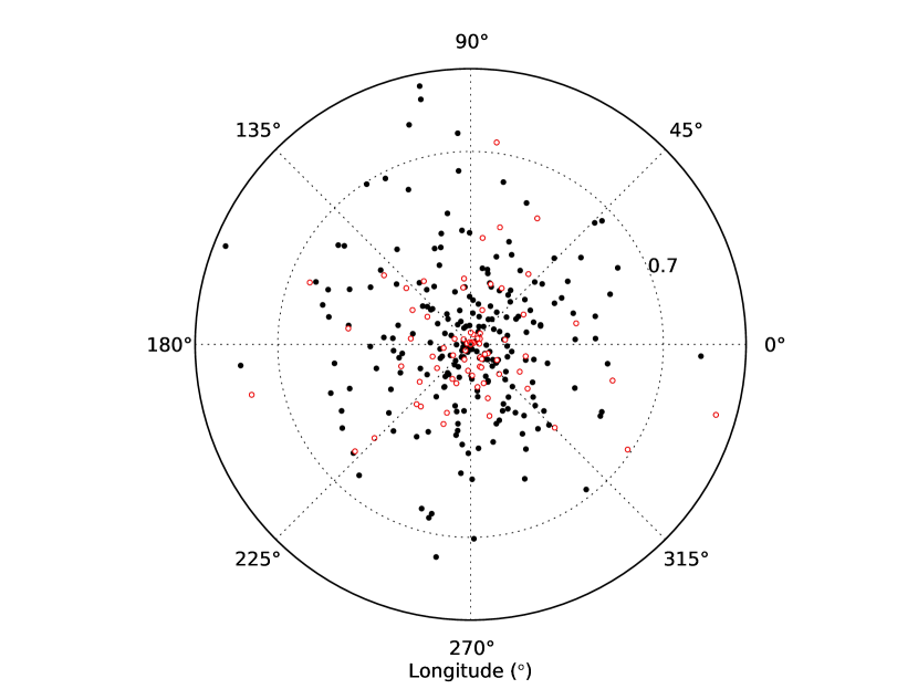
Figure 1: Polar plot showing the positions of the sample stars projected onto the Galactic plane. The radius is limited to 1 kpc and the concentric dotted circle represents the distance of 0.7 Kpc, within which $\sim$80% of the stars in our sample are located. The open red circles are spectroscopic binaries/multiple systems identified in our sample. Values for distance of the stars are more uncertain beyond 0.5 kpc of the Sun.

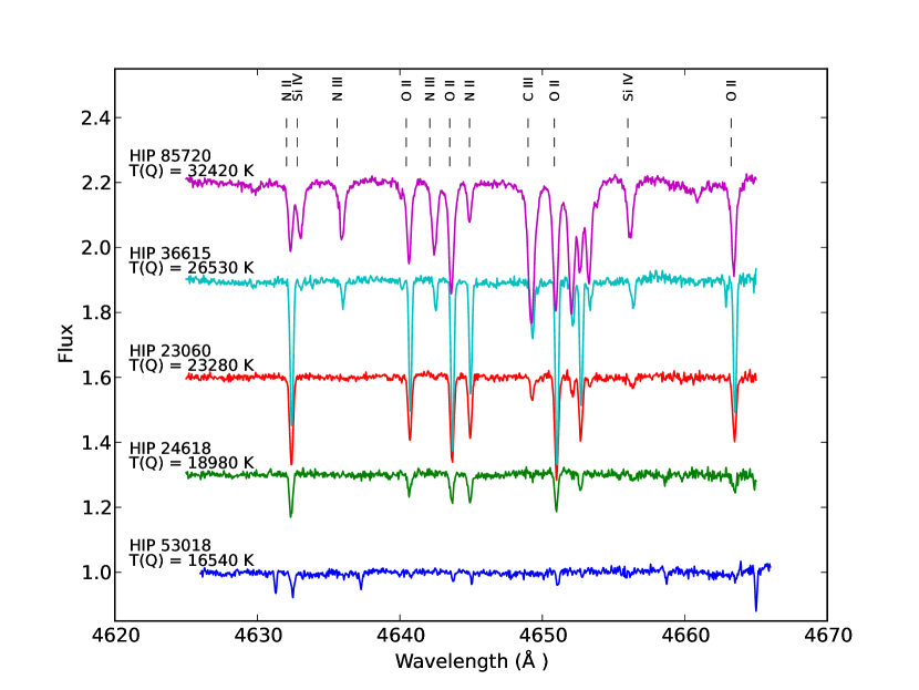
Figure 2: Example spectra of five sample stars in the region $\lambda\lambda 4625-4665$ Å. Some spectral lines are identified. The spectra were arbitrarily displaced in intensity for better viewing.

3 Stellar Characterization

3.1 Identification of Spectroscopic Binaries

It is likely that most massive OB stars form in clusters or associations, with the probability of a star forming with a companion being high. The recent study by Oudmaijer & Parr (2010), for example, found a binary fraction of $\sim 30\%$ in their photometric survey of B and Be stars. A first objective in this study is to identify those stars, among the 350 stars observed, that show spectral signatures of binary or multiple components. This was done through a careful visual inspection of their spectra. Single-line spectroscopic binaries are not detected here, as the spectra are only from single epoch observations. Spectroscopic binaries will be discarded from further analysis in this study since the methodology here is most appropriate for spectra showing a single component.

Some stars in our sample were identified as clearly having double, multiple or asymmetric spectral lines. In addition, some stars in our sample which were found to be binary or multiple systems in the large survey of stellar multiplicity within the HIPPARCOS catalogue by Eggleton & Tokovinin (2008) and/or appeared as binaries in the study of OB star variability based on HIPPARCOS photometry by Lefèvre et al. (2009). Table 1 lists 78 stars culled from the sample as spectroscopic binaries or multiple systems, representing 22% of the stars in our sample. Column 1 has the star identification, column 2 lists the spectral types from SIMBAD. In column 3 stars are classified as ‘SB’, if they were found here to be a spectroscopic binary or multiple system and ‘asym’, if they exhibited asymmetric line profiles; ET08 and Lef09 if they were in Eggleton & Tokovinin (2008) or Lefèvre et al. (2009). The stars in Table 1 will not be analyzed in the remainder of this paper.

3.2 Spectral Types and Effective Temperatures

The spectral types of the stars were determined based on the classification system presented in the Atlas of OB stars by Walborn & Fitzpatrick (1990). Relative intensities of some key absorption line ratios such as: $\lambda 4471$ He i / $\lambda 4481$ Mg ii; $\lambda 4630$ N ii / $\lambda 4631$ Si iv; $\lambda 4641$ N iii / $\lambda 4643$ N ii, and $\lambda 4649$ C iii / $\lambda 4650$ O i were used to assign spectral types. In order to map the Walborn & Fitzpatrick spectral types into our sample, a small grid of non-LTE synthetic spectra of two spectral regions, $\lambda\lambda$4450 – 4490 Å and $\lambda\lambda$4630 – 4700 Å  were computed for $T_{eff}$’s between 15,000 – 33,000K, logarithmic of the surface gravity $\log g=4.0$, and solar composition. The theoretical spectra were calculated with the codes TLUSTY and SYNPLOT (Hubeny 1988; Hubeny & Lanz 1995). The Walborn & Fitzpatrick standard star spectra were then visually matched to their closest synthetic counterpart in the grid; spectral types assigned as O9, B0, B1, B2, B3, B4 and B5 were found to correspond to model spectra with $T_{eff}$’s of 33,000K; 30,000K; 25,000K; 20,000K; 18,000K; 16,000K and 15,000K, respectively.

Synthetic and observed spectra were then compared by visual inspection in order to assign spectral types for the target stars. The goal was simply to determine an appropriate spectral type to each star, and not to match in detail the observed and theoretical spectra in a fine analysis. Since a fraction of the stars in our sample have spectral lines somewhat blended by rotation, synthetic spectra were convolved for $v\sin i$ (in steps of $v\sin i=50$ km s^-1) in order to aid in the assignment of spectral types of broad lined stars. Spectral types for the target stars are listed in Table 2 (column 2).

Effective temperatures for the stars were estimated from a calibration of the classical reddening free parameter $Q$ (Johnson 1958; $Q=(U-B)-X\cdot(B-V)$, where $X=E(U-B)/E(B-V)$). In order to estimate $T_{eff}$ for the sample stars in this study we will adopt the $T(Q)$ calibration presented in Massey et al. (1989) and defined below:

$$\log T_{eff}=3.994-0.267\cdot Q+0.364\cdot Q^{2}.$$ (1)

A $T(Q)$ calibration has also been proposed by Daflon et al. (1999). However, a large number of stars in the sample studied here are much cooler than the validity range of the Daflon et al. calibration. Figure 3 shows as a solid blue line the calibration by Massey et al. (1989) for the $Q$-interval of the stars in this study. The calibration by Daflon et al. (1999) is also shown in Fig. 3 as black dashed line, for comparison. The average differences between the two calibrations are relatively small: $\langle\Delta T_{eff}\rangle=-380$ K and $\sigma=177$ K, for $Q$-values ranging between $-0.62$ and $-0.87$; and $\langle\Delta T_{eff}\rangle=+583$ K and $\sigma=405$ K for $Q$-values between $-0.61$ to $-0.53$. Effective temperatures for those stars with measured radius from Code et al. (1976) are shown by red circles in Fig. 3. The overall agreement of the Code et al. (1976) results with the calibrations is generally good but with significant scatter, which is indicative of the uncertainties when using the $Q$-index as a temperature indicator. More recently, Paunzen et al. (2005) also presented a calibration for the $Q$-index with the effective temperature and the $T\times Q$ relation in that study is quite similar to the one derived in Massey et al. (1989).

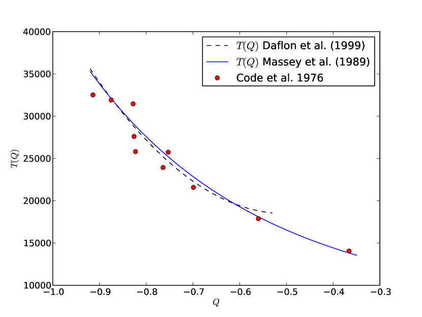
Figure 3: The T(Q) calibration from Massey et al. (1989, solid blue line) which was adopted in this study to estimate effective temperatures for the target stars. The Q-index calibration from Daflon et al. (1999) is also shown for comparison (black dashed line). The red filled circles represent the stars with measured radius and effective temperatures in Code et al. (1976).

The Johnson color indices $(U-B)$ and $(B-V)$ for the studied stars were obtained from Mermilliod (1987). For those 57 stars in the sample without published Johnson photometry, UBV colors were computed from Strömgren photometry from Hauck & Mermilliod (1980, 1998), using the transformation in Harmanec & Božić (2001). In addition, there were 41 remaining stars in our sample for which there was no available photometry in the literature, and in those cases we relied on spectral types in order to obtain the intrinsic colors from the tables in Fitzgerald (1970) and then estimate $Q$. In columns 3, 4, and 5 of Table 2 we list the $V$ magnitudes, the $Q$ parameters, and the derived $T_{eff}$’s for 272 stars of the observed sample. The estimated $T_{eff}$’s here are good for the purpose of a rough stellar characterization of our sample and, in particular, these suffice for a solid derivation of $v\sin i$ values since the grid of synthetic spectra used here (Sect. 4) has been computed for steps of 5,000 K in $T_{eff}$.

4 Projected Rotational Velocities

Projected rotational velocities for the targets were estimated from measurements of the full width at half maximum (FWHM) of 3 He i lines at $\lambda 4026$ Å, $\lambda 4388$ Å and $\lambda 4471$ Å. The FWHMs of the He i line profiles were measured using the IRAF package splot, using a procedure consistent with that adopted in Daflon et al. (2007): the continuum level was marked at the line center, and the half-width of the red wing was measured at the half-maximum and then doubled in order to derive the FWHM. Figure 4 shows examples of the sample He i lines for the observed stars HIP 73624 (black continuous line) and HIP 33492 (red dashed line).

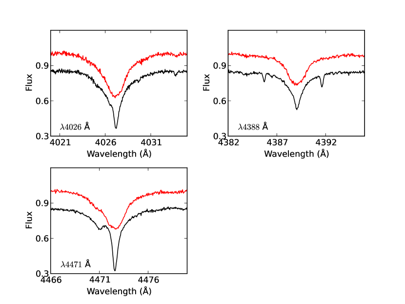
Figure 4: Sample spectra showing the 3 He i lines that were used to derive the projected rotational velocities for the target stars. The bottom spectra (black) in the three panels are for the star HIP 73624 with $v\sin i=17$ km s^-1 and the top spectra (red) are for the star HIP 33492 with $v\sin i=71$ km s^-1. The spectra were arbitrarily displaced in intensity for better viewing.

The measured FWHM were converted to $v\sin i$’s via interpolating in the grid of synthetic FWHM of He i lines presented in Table 2 of Daflon et al. (2007) for the adopted effective temperature of each star. The synthetic He i profiles in that study were computed in non-LTE using the codes DETAIL (Giddings, 1981) and SURFACE (Butler & Giddings, 1985) and were based on the helium model atom described in Przybilla (2005). We note that the macroturbulent velocity was kept as zero in the calculation of the synthetic profiles by Daflon et al. (2007) but it is likely to result in additional broadening of the line profiles. Simón-Díaz et al. (2010) did a careful analysis and disentangled the effects of macroturbulence and rotation in line profiles by using Fourier Transform method and obtained macroturbulent velocities for early B-type dwarfs that are generally lower than 20 km s^-1, with a clear trend of decreasing for late B-types. In order to test the importance of neglecting macroturbulence in the synthetic FWHM of the He lines we did a test calculation including a gaussian macroturbulent velocity of 20 km s^-1. The results indicate that considering the uncertainties of the method adopted here, including macroturbulence at this level has negligible effect in the measured FWHM of the synthetic spectra of sample He i lines.

The measured values of FHWM for the 3 He i lines used in the $v\sin i$ determinations are found in Table 2 (columns 6, 7, and 8); columns 9, 10 and 11 list the $v\sin i$’s for each He line; columns 12 and 13, the final $v\sin i$ values for the studied stars: these represent the average values and the standard deviations in each case. We note that $v\sin i$’s were not derived for 6 stars with $T_{eff}$’s higher than 33,700 K, as they fell out of the validity of the $v\sin i$ calibration from Daflon et al. (2007).

Figure 5 shows a comparison of the $v\sin i$ results in this study with those from other determinations in the literature: results from Abt et al. (2002) are represented as filled blue circles while results from the Wolff et al. (2007) study are represented as red filled triangles. Abt et al. (2002) derived $v\sin i$ for a sample of B stars of The Bright Star Catalogue with luminosity classes between I and V, using a calibration for FWHM of He i and Mg ii lines anchored on standard stars of Slettebak et al. (1975). Wolff et al. (2007) obtained a relationship between FWHM and $v\sin i$ based on results from He i lines of Huang & Gies (2006). We note that the $v\sin i$’s for the stars in common with Abt et al. (2002) are systematically lower than the ones here in the range between $\sim$ 0 – 90 km s^-1 ($\langle\Delta v\sin i\rangle$(This Study – Abt et al)$=9$ km s^-1 for 24 stars in common); higher than ours in the range between 90 – 150 km s^-1 ($\langle\Delta v\sin i\rangle$(This Study – Abt et al.)$\geq-15$); and in rough agreement for the largest $v\sin i$ (except for one star). The $v\sin i$’s in Wolff et al. (2007) are mostly higher than ours, except for stars with the lowest $v\sin i$’s. The average $v\sin i$ difference (This study – Wolff et al.) is $-26$ km s^-1 for 17 stars in common. Given the uncertainties in the determinations and the methods adopted, there is reasonable agreement between the three different studies.

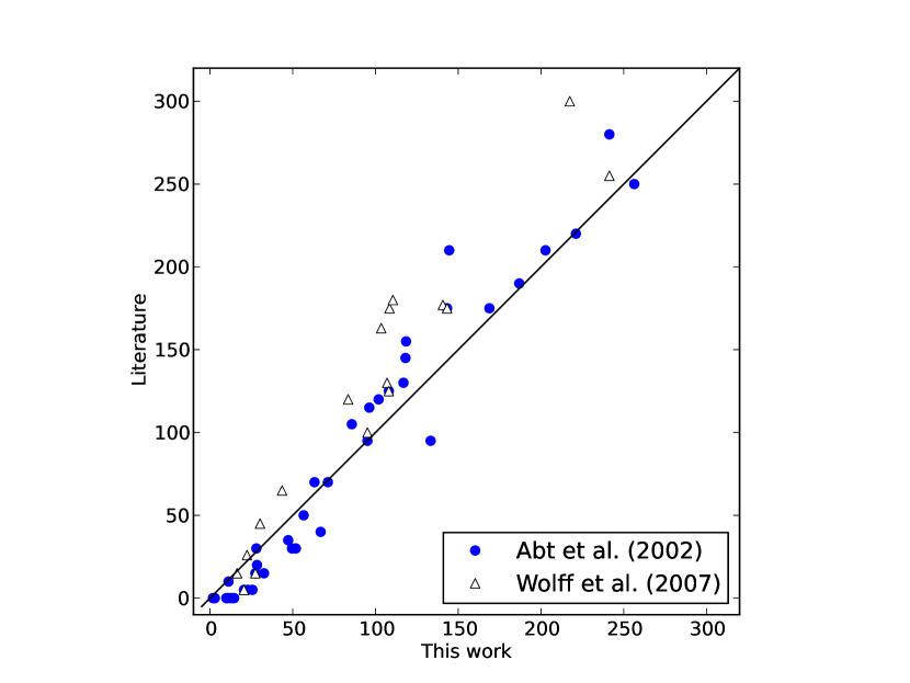
Figure 5: A comparison between the $v\sin i$’s derived in this study for stars in common with other two studies in the literature: Abt et al. (2002) (blue circles) and Wolff et al. (2007) (white triangles). The solid line represents the locus of equal values.

5 Discussion

5.1 The Entire Sample

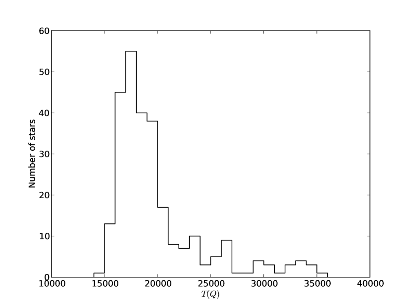
Figure 6: Histogram showing the distribution of effective temperatures for the studied sample.

We start our discussion by showing results for the derived effective temperatures for the stars. A histogram showing the distribution of effective temperatures for 272 OB stars is shown in Fig. 6. The effective temperatures of the targets sample peak around 17,000K, with most stars being cooler than 28,000K.

Figure 7 illustrates the box plots for the $v\sin i$ values for the studied stars in each corresponding spectral type. The box extends from the lower to upper quartile values of the data, with a line at the median and a small box as the mean. The whiskers extend from the box to show the range of the data. The crosses are the outliers. An inspection of this figure indicates that the mean $v\sin i$ for each spectral type bin is roughly consistent with a constant value across spectral type. The average $v\sin i$ value computed for the studied sample is $98$ km s^-1. Huang & Gies (2006) also found a distribution of mean $v\sin i$ for cluster stars which is basically flat over a similar spectral type range, although their study also includes giant stars. Overall the mean $v\sin i$’s obtained here for spectral types bins B0–B2 and B3–B5 are in rough agreement with the average results for luminosity classes IV and V in Abt et al. (2002). (see Sect. 4 for comparisons the $v\sin i$ for stars in common in the two studies).

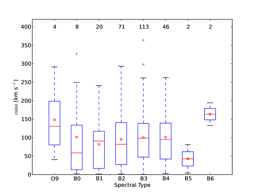
Figure 7: Box plot for the studied stars in terms of the spectral type. The average $v\sin i$ for the stars in each spectral type bin is roughly constant, even considering the least populated bins.

The $v\sin i$ distribution of the current sample of 266 O and B stars is shown in top panel of Fig. 8. The distribution has a modest peak at low $v\sin i$’s ($\sim$ 0 – 50 km s^-1) but it is overall flat (a broad distribution) for $v\sin i$’s roughly between 0 – 150 km s^-1; the number of stars drops for higher values of $v\sin i$. As previously mentioned, the targets in this study were selected considering only their spectral types in the HIPPARCOS catalogue. The sample studied here includes both stars in clusters and OB associations, as well as isolated stars that can represent some sort of field population.

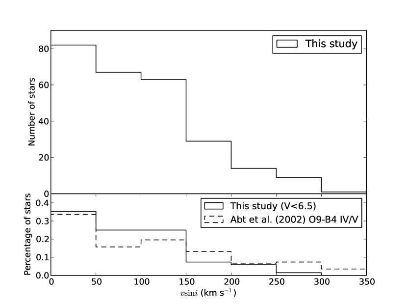
Figure 8: Histogram of $v\sin i$ distribution of our sample on the top panel. The bottom panel compares the normalized distribution of a subsample of stars in our sample with a magnitude cut in $V=6.5$ and a sample with 312 field stars (spectral types O9–B4IV/V) culled from Abt et al. (2002).

One of the difficulties in making meaningful comparisons between rotational velocity distributions of stars in clusters versus stars in the ‘field’ is in defining what constitutes a ‘field’ star sample. This discussion is, in fact, related to the question of whether OB stars can form in isolation and if all OB stars, although isolated, belonged in the past to a cluster. The initial idea was that OB stars were only formed in clusters and associations but later on were ejected or dispersed into the Galactic field. There is growing evidence, however, that at a least a small fraction of the O stars may be born in isolation (or from small molecular clouds). For instance, Krumholz et al. (2009) used a 3-D hydrodynamic simulation to show that the formation of isolated massive stars is possible; they successfully form a massive binary (having 41.5 M_⊙ and 29.2 M_⊙) from a 100 M_⊙ molecular gas. One strong observational evidence that field OB stars may form in situ was presented by Lamb et al. (2010), who found very low mass companions around apparently isolated field OB stars in the SMC. Indeed, Oey & Lamb (2011) cite several lines of empirical evidence to suggest that in situ field massive stars constitute a significant, and perhaps dominant, component of the field OB star population.

Although samples of field stars are contaminated at some level with stars that are in the field now but were born in dense environments, a comparison of the $v\sin i$’s obtained for the entire sample studied here with other samples taken as representative of the field population is of interest. Abt et al. (2002) provide the cornerstone work of the distributions of projected rotational velocities of the so-called field OB stars. The targets in that study were taken from The Bright Star Catalogue and also include stars that are members of clusters and associations. For the sake of comparison with a field sample that is representative of the spectral types and luminosity classes of most of the studied stars, we culled from the Abt et al. (2002) sample those stars with spectral types O9 – B4 and luminosity classes IV and V. The distribution of $v\sin i$’s for this subsample is shown as the dashed line histogram in the bottom panel of Fig. 8. We thus selected those stars of our sample with $V<6.5$ which is the magnitude limit of The Bright Star Catalogue (Hoffleit & Jaschek 1982) and this subsample is also presented in the the bottom panel of Fig. 8. A Kolmogorov-Smirnov test gives more than 90% of probability that both distributions are drawn from the same population. These results suggest that the $v\sin i$ distribution obtained from Abt et al. (2002) for the so-called field population is similar from the $v\sin i$ distribution of our sample brighter stars.

5.2 Stars in OB Associations and Clusters

The idea that stellar rotation of OB stars in clusters relates to cluster density has been put forward in previous studies in the literature. In particular, comparisons between the $v\sin i$ distributions of stars from clusters, OB associations, or the field have shown that stellar members of dense associations or clusters rotate on average faster than member stars of unbound associations or the field (e.g. Wolff et al. 2007; Daflon et al. 2007). Previous studies discussing rotational velocity distributions of stars in clusters include Guthrie (1982); Wolff et al. (1982, 2007); Huang & Gies (2006, 2008); Huang et al. (2010). In general, all these studies confirm that there seems to be real differences between the $v\sin i$ distributions of cluster members when compared to field; there are fewer slow rotators in the clusters when compared to the field, or, the stars in clusters tend to rotate faster. Guthrie (1982), however, found the presence of a bimodality in his $v\sin i$ distribution: the cluster distribution was double peaked with one at $v\sin i<50$ km s^-1 and the other at $V\sin i\sim 225$ km s^-1.

A comparative study of the $v\sin i$’s of all stars in our sample in connection with their birth environments (clusters/associations or field) is of interest but firmly establishing membership is a difficult task as detailed and careful membership determinations are beyond the scope of this paper. Instead, in this study, we use literature results in order to select a subsample of stars for which there is secure information on their membership. For OB associations, this is based on the list of probable members from the census of OB associations in the Galactic disk from the HIPPARCOS catalogue by de de Zeeuw et al. (1999); and in the study of the stellar content of the Orion association by Brown et al. (1994). In addition, we searched the target list in Humphreys & McElroy (1984) and found a few more targets to be association members. The stars in our sample members in higher density environments or clusters were obtained from cross checking the studied sample with the WEBDA open cluster database (Mermilliod & Paunzen 2003). In addition, we searched the open cluster member list of Robichon et al. (1999). The membership information for each star can be found on column 15 of Table 2.

Histograms showing the $v\sin i$ distributions for the culled subsamples of OB association and cluster members are shown in Fig. 9 (red dashed lined histograms). The black solid histograms represent a larger sample combining our sample with the sample of O and B stars from Daflon et al. (2007). In that paper, 143 OB stars members of open cluster, OB associations and 23 stars in H ii regions have been observed in order to probe the radial metallicity gradient in Galactic disk. Since the $v\sin i$’s in the present study were derived using the same grid and methodology as in Daflon et al. (2007), the discussion beyond this point will be based on the combined sample (black solid histograms) given better statistics. The distribution of $v\sin i$’s obtained for the stars in OB associations (top panel) has a relatively larger number of objects with $v\sin i$’s between 0 – 50 km s^-1 and the number of stars declines smoothly with $v\sin i$. For stars in clusters (bottom panel) there is a smaller fraction of slow rotating stars and an apparent peak at 50 –100 km s^-1. The smooth distribution of $v\sin i$ values for the association members may result from a nearly single values for equatorial rotational velocity that is viewed at random inclination, while the cluster distribution may be more complex.

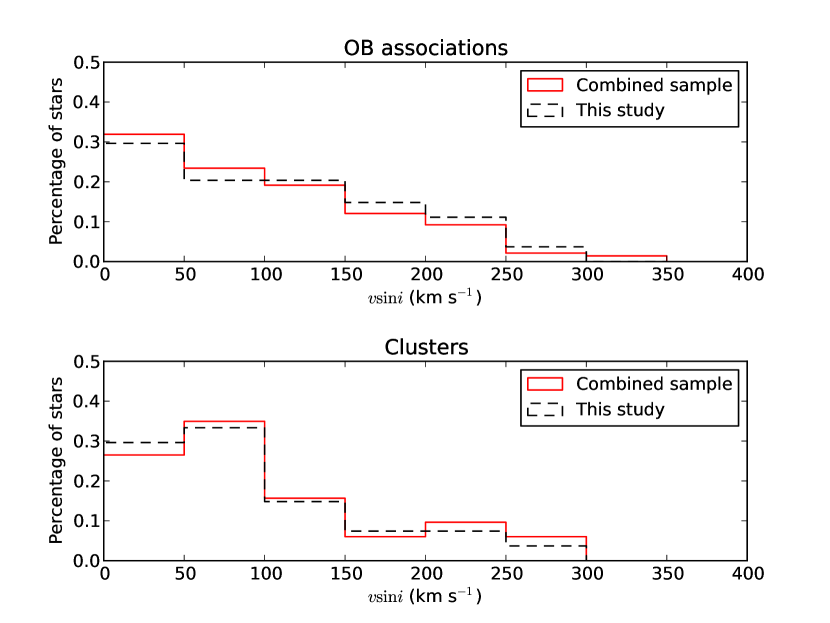
Figure 9: Distribution of $v\sin i$’s for the studied samples of OB association (top panel) and cluster members (lower panel) are shown as red dashed lined histograms. The black solid line histograms represent the combined sample: stars in this study plus 143 star members of clusters and associations from Daflon et al. (2007). Both studies use the same methodology to derive $v\sin i$.

Figure 10 shows a comparison of the cumulative fractions for the $v\sin i$ distributions for the clusters and OB associations, as well as the field (from the subsample selected here from Abt et al. (2002) as discussed above). The field sample has a higher fraction of slowly rotating stars ($v\sin i$ between 0 and 50 km s^-1) when compared to the OB associations or clusters. In addition, there is a clear excess of stars with $v\sin i$’s between roughly 70 – 130 km s^-1 in the cluster distribution when compared to the OB associations as well as the field. In fact, there seems to be a gradation from cluster to OB association to field confirming the trend found by Wolff et al. (2007). A Kolmogorov-Smirnov test between the field star sample and the association sample gives 92 percent probability that both samples are drawn from distinct populations and 88 percent probability that the cluster and the field are drawn from distinct populations. A K-S test between the OB associations and the clusters distributions, however, gives only a 50 percent probability that these are drawn from distinct populations. Thus, any differences between the distributions of clusters and associations in this study are not so clear and may not be statistically significant; larger studies are needed.

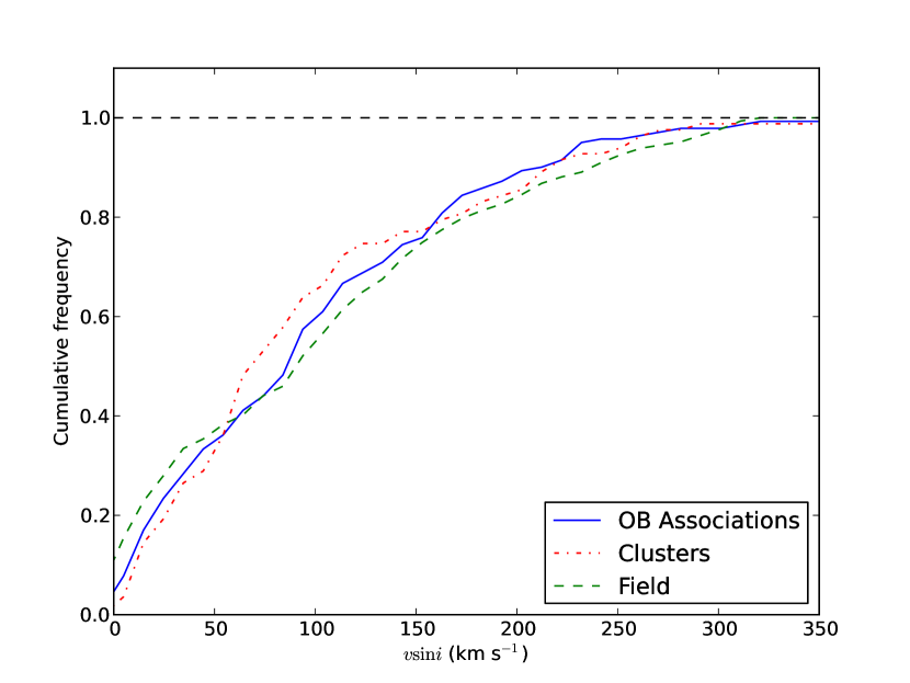
Figure 10: Cumulative fractions for the $v\sin i$ distributions for the clusters, OB associations and the field. There seems to be a gradation from cluster to OB association to field. A K-S test between the field star sample and the association sample gives 92 percent probability that both samples are drawn from distinct populations and 88 percent probability that the cluster and the field are drawn from distinct populations. A K-S test between the OB associations and the clusters distributions, however, gives only a 50 percent probability that these are drawn from distinct populations.

5.3 Runaway Stars

Few studies in the literature have investigated the distribution of rotational velocities in runaway OB stars. Martin (2006) studied the properties of a population of stars far from the Galactic plane and this included a sample of 21 Population I runaway stars. The $v\sin i$ distribution for the runaway stars was found in that study to be broad with no apparent peaks in the range $v\sin i=50$ to 200 km s^-1 and with a slight decline for values of $v\sin i$ below 50 km s^-1 (see Martin 2006, Fig. 9b). The interpretation was that the projected rotational velocity distribution for the runaways was more similar to that of an OB association than to the field; one of the main distinctions when comparing with the field is the absence of a larger number of slow rotators in the distribution of the runaway sample.

Runaway stars can be explained by two scenarios: the binary supernova scenario, in which a star is ejected from the binary system when its companion turns into a supernova, and the dynamical ejection scenario, in which a star is ejected from its parent cluster or association due to dynamical processes. These objects are usually identified via one of three methods: spatial velocities, tangential velocities, or radial velocities. Tetzlaff et al. (2011) combined these three methods to identify runaway stars in the HIPPARCOS catalogue. Our study has 34 stars identified as runaways in Tetzlaff et al.’s catalogue of runaway candidates.

The $v\sin i$ distribution obtained for the runaway stars in our sample is shown as a solid line histogram in Fig. 11. Two peaks are evident from a visual inspection of our distribution: one corresponding to slow rotating stars (or, $v\sin i\sim$ 0 – 50 km s^-1) and another corresponding to higher projected rotational velocities ($v\sin i$’s between 100 – 150 km s^-1). We also show for comparison a histogram representing the combined sample including the runaway stars studied by Martin (2006). Given that the distribution of $v\sin i$ in Martin (2006) runaway sample is generally flat, the two $v\sin i$ peaks observed in the solid line histogram remain in the combined sample.

A K-S test was run on the runaway $v\sin i$ distribution obtained in this study compared to the other 3 samples discussed previously: the field, the OB association and the cluster subsamples. The probabilities that both distributions are drawn from the same populations are 18 percent, 40 percent and 71 percent, respectively for the field, association and cluster. This is an indication that the runaway phenomenon maybe more likely associated with the dense cluster environments, as expected from a dynamical ejection scenario.

However, we note the lack of very massive and dense clusters nearby the Sun, which are the main sources of runaways ejected by means of the dynamical ejection scenario.

As a final note, the presence of a second peak at low $v\sin i$ ($\sim$ 0 –50 km s^-1) in the runaway distribution in this study, could be related to runaways originating from OB associations. As discussed previously, stars in associations have tipically lower $v\sin i$ when compared to cluster stars.

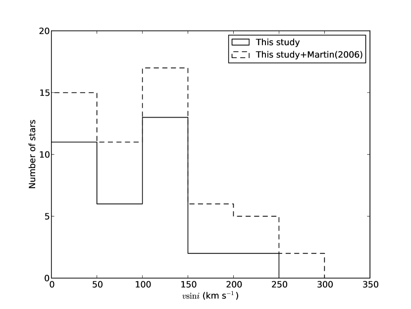
Figure 11: $V\sin i$ distribution for the runaway stars in our sample is shown (solid line histogram). The distribution has two peaks. A KS-test indicates that the runaway $v\sin i$ distribution is more similar to the cluster distribution. This could be an indication that the runaway stars originated from a dynamical ejection scenario. The presence of a second peak at low $v\sin i$ could be related to runaways ejected from OB associations. A histogram representing the combined sample including the runaway stars studied by Martin (2006) is also presented for comparison (dashed line histogram).

6 Conclusions

High resolution spectroscopic observations and a first characterization of a sample of 350 OB stars has been carried out. Projected rotational velocities were obtained for 266 stars (after rejecting spectroscopic binaries/multiple systems) using measurements of FWHM of He i lines and interpolation in a synthetic grid from Daflon et al. (2007). The $v\sin i$ distribution obtained for the studied sample has a modest peak at low $v\sin i$’s ($\sim$ 0 – 50 km s^-1) but it is overall flat for $v\sin i$’s roughly between 0 – 150 km s^-1; the number of stars drops for higher values of $v\sin i$. The $v\sin i$ distribution of our brighter sample stars is similar to the one obtained from a sample of field stars picked from the work of Abt et al. (2002).

Literature results on membership were used in order to identify subsamples of stars belonging to OB associations or clusters. We compared these two groups and found that stars members of OB associations and clusters compose two distinct populations. The cluster stars tend to have higher $v\sin i$’s when compared to the OB association subsample which could mean that stellar rotation of a population is dictated by the density of the cloud in which it forms. Also, when the OB association and cluster populations are compared with the field sample, it is found that the latter has a larger fraction of slowest rotators, as previously shown by other works. In fact, there seems to be a gradation from cluster to OB association to field in $v\sin i$ distribution.

The present sample has 34 stars that were identified as runaway candidates in Tetzlaff et al. (2011) catalogue. The $v\sin i$ distribution of the runaways sample presents two peaks: one for $v\sin i\sim$ 0 – 50 km s^-1 and another for $v\sin i\sim$ 100 – 150 km s^-1. The K-S test run with the runaway stars, OB association, cluster and field samples indicate that the runaway $v\sin i$ distribution is more likely to be similar with the distribution of the denser environments, which could suggest that these stars were ejected through the dynamic ejection mechanism. Also, there is a possibility that the low $v\sin i$ peak is composed of stars that were ejected from OB associations.

Table 1:

HIP	Spec. Type	Bin.
17563	B3V	Lef09, ET08
17771	B3V	ET08
21575	B3V	SB, Lef09
22663	B2/B3V	Asym., Lef09
25028	B3V	SB, ET08
25066	B3V	SB
25142	B2	SB, ET08
26063	B3V	Lef09, ET08
26213	B3V	SB
28142	B2V	SB?, Lef09
28756	B2.5V	Lef09, ET08
29126	B1V	asym:
29321	B2V	SB, Lef09
31068	B3V	SB, Lef09
31190	B2IV	SB, Lef09, ET08
31593	B3V	Asym.?, Lef09
31959	B3V	SB
32810	B6Vnpe	SB, Lef09, ET08
33330	B3V	SB
33723	O9V	SB
33971	B1V	Lef09, ET08
34579	B2V	Lef09, ET08
34817	B3V	Asym., ET08
35202	B4V	SB, ET08
35611	B2.5V	Asym., Lef09, ET08
35621	B2V	asym.
36363	B5Vp	SB, ET08
37450	B5V	SB, ET08
37502	B2V	SB
37524	B5V	SB?
37668	B4V	SB
37784	B2V	SB
38020	B1.5IV	SB, ET08
38455	B2.5V	Lef09, ET08
39943	B4V	ET08
39992	B4V	SB
40341	B1.5V	SB
40443	B4V	SB
41039	B1V	SB ET08
41250	B3V	SB, Lef09, ET08
41296	B2Ve	ET08
41515	B3V	SB, Lef09, ET08
41621	B2Vne	SB ET08
43955	B2IV	asym.
46296	B2/B3IV	SB
47559	B4V	SB, ET08
49695	B4V	SB
50780	B3V	SB, Lef09
52370	B4V	SB?, Lef09, ET08
53089	B3V	SB
55350	B4V	SB
57669	B3Vne	Lef09, ET08
59449	B3V	Asym., ET08
60905	B3IV/V	SB
62322	B2.5V	ET08
64719	B4V	SB
65271	B3V	ET08
67042	B3V	SB
69648	B3V	asym.
74117	B3V	SB, ET08
74680	B3V	SB
77811	B3V	SB, ET08
77939	B2/B3V	ET08
78004	B3/B4V	SB
78168	B3V	SB?, Lef09, ET08
78821	B2V	SB, ET08
79404	B2V	ET08
80405	B4V	SB
88993	B1V	SB
90804	B2V	SB, Lef09, ET08
91352	B2V	SB
92470	B2IV	asym.
92989	B8IVs…	SB, Lef09, ET08
93225	B4V	SB ET08
93502	B2V	SB, Lef09
93732	B3V	SB, Lef09
99457	B1V	SB, Lef09
100881	B4V	SB, ET08

Note. — The columns are: (1) The HIPPARCOS identification, (2) the spectral type, (3) Binarity/multiplicity: We classified the star as “asym.” when it has an asymetric line profile or “SB” when it is a spectroscopic binary. Some stars are listed as binaries in Lefèvre et al. (2009) (Lef09) and/or Eggleton & Tokovinin (2008) (ET08).

Note. — Table 1 is published in its entirety in the electronic edition of the Astrophysical Journal.

Table 2:

HIP	Spec. Type	$V$	$Q$	$T_{eff}$	FWHM			$v\sin i$			$\langle V\sin i\rangle$	$\sigma(V\sin i)$	N	Memb.
				(K)		(Å)			(km s-1)		(km s-1)	(km s-1)
					$\lambda 4026$Å	$\lambda 4388$Å	$\lambda 4471$Å	$\lambda 4026$Å	$\lambda 4388$Å	$\lambda 4471$Å
(1)	(2)	(3)	(4)	(5)	(6)	(7)	(8)	(9)	(10)	(11)	(12)	(13)	(14)	(15)
14898	B5V	7.03	-0.41	14610	$\cdots$	1.0	0.7	$\cdots$	5	4	4	1	2	R
15188	B3Ve	7.96	-0.53	17290	4.2	3.9	3.7	153	151	118	141	19	3	R
16466	B4V	9.32	-0.51	16780	1.7	1.5	1.0	22	30	$\cdots$	26	5	2	R
18926	B3V	6.45	-0.62	19930	5.7	5.7	5.4	234	235	194	221	23	3	$\cdots$
18957	B3V	5.31	-0.5	16540	1.8	1.6	1.2	28	33	23	28	5	3	$\cdots$
20884	B3V	5.53	-0.48	16070	1.4	1.4	0.9	15	$\cdots$	11	13	3	2	A
23060	B2V	6.13	-0.71	23280	2.1	1.3	1.1	31	20	$\cdots$	26	8	2	R
23364	B3V	4.81	-0.61	19600	2.5	2.1	1.8	52	60	44	52	8	3	$\cdots$
24618	B2V	6.53	-0.59	18980	1.6	1.3	1.0	6	16	$\cdots$	11	6	3	$\cdots$
25368	B3V	6.42	-0.59	18980	3.0	2.7	2.6	82	91	77	84	7	3	A
25480	B4V	6.62	-0.6	19290	5.6	5.0	5.9	230	203	219	217	14	3	A
25493	B2V	6.73	-0.6	19290	3.4	3.0	3.5	100	106	104	103	3	3	A
25496	B3V	7.19	-0.52	17030	2.2	1.9	1.5	45	48	38	44	5	3	A.R
25582	B2V	6.38	-0.63	20260	1.4	1.4	1.1	$\cdots$	21	$\cdots$	21	$\cdots$	1	A.R
25751	B2V	5.74	-0.7	22870	3.2	3.0	3.6	98	114	112	108	9	3	A.R
25844	B3V	7.63	-0.57	18380	1.9	1.8	1.3	22	$\cdots$	22	22	1	2	$\cdots$
25850	B2V	7.95	-0.68	22070	3.4	3.2	3.8	104	123	120	116	10	3	A
25869	B2V	6.20	-0.61	19600	2.1	1.6	1.2	23	32	$\cdots$	27	7	2	A
25881	B3V	7.56	-0.52	17030	1.8	1.8	1.4	27	$\cdots$	33	30	4	2	A
25923	O9V	4.62	-0.92	35300	$\cdots$	$\cdots$	$\cdots$	$\cdots$	$\cdots$	$\cdots$	$\cdots$	$\cdots$	0	$\cdots$
26093	B3V	5.59	-0.53	17290	3.6	3.4	3.5	118	129	109	118	10	3	C
26098	B2V	6.57	-0.68	22070	3.9	3.8	4.3	135	151	145	143	8	3	A.R
26166	B3V	6.71	-0.59	18980	3.4	3.8	3.7	102	$\cdots$	115	108	9	2	A
26258	O9V	6.87	-0.88	32420	4.0	4.1	4.5	161	173	169	168	6	3	C
26439	B4V	7.09	-0.49	16300	3.0	2.6	2.9	93	88	94	92	3	3	A
26508	B2V	6.81	-0.64	20600	5.7	5.5	6.5	236	224	248	236	12	3	A
26581	B3V	7.55	-0.45	15410	3.3	3.0	3.1	113	108	100	107	7	3	A.R
26785	B2V	7.63	-0.61	19600	2.5	1.8	1.6	48	47	34	43	8	3	A
26876	B4V	8.90	-0.54	17550	5.2	5.3	5.8	203	217	214	211	7	3	A
27103	B3V	6.76	-0.6	19290	3.0	2.8	3.4	80	99	100	93	11	3	$\cdots$
27937	B3V	6.09	-0.51	16780	1.9	1.5	1.3	30	28	28	29	1	3	$\cdots$
28973	B3V	6.64	-0.56	18100	2.2	1.9	1.8	41	51	49	47	6	3	A
29121	B3Vn	8.79	-0.64	20600	8.0	8.9	8.8	355	375	361	364	10	3	C
29127	B1V	8.33	-0.7	22870	1.9	1.4	1.3	18	$\cdots$	17	17	1	2	C
29201	B0Ve	8.58	-0.85	30480	5.3	6.0	6.4	233	255	261	249	15	3	R
29213	B4V	7.96	-0.54	17550	4.5	4.4	4.9	165	174	171	170	5	3	R
29387	B3V	8.61	-0.6	19290	4.2	4.2	4.6	150	166	154	157	8	3	$\cdots$
29417	B2V	5.05	-0.64	20600	1.6	1.0	1.0	0	3	$\cdots$	2	2	2	A.R
29429	B1V	7.05	-0.67	21690	3.1	2.5	3.0	85	87	88	87	1	3	$\cdots$
29446	B2V	7.49	-0.54	17550	2.8	2.6	3.1	78	87	94	86	8	3	$\cdots$
29678	B1V	5.89	-0.79	27050	1.7	1.1	1.0	11	16	$\cdots$	14	3	2	R
29771	B2/B3Ve	5.96	-0.63	20260	6.1	6.2	6.6	257	256	256	256	1	3	$\cdots$
29941	B2/B3V	5.49	-0.58	18680	2.6	2.2	2.6	58	65	78	67	11	3	$\cdots$
30143	B1.5Ve	5.53	-0.76	25540	5.4	5.8	6.3	228	246	249	241	11	3	R
30382	B3V	6.38	-0.52	17030	1.4	1.2	0.8	11	9	$\cdots$	10	2	2	$\cdots$
30468	B4Ve	6.12	-0.57	18380	1.9	1.6	0.8	21	35	$\cdots$	28	10	2	$\cdots$
30700	B4V	6.49	-0.44	15200	5.5	5.9	6.0	220	246	222	229	15	3	C
30739	B3V	8.80	-0.6	19290	3.2	3.0	3.4	90	107	102	99	9	3	$\cdots$
30743	B4V	7.49	-0.54	17550	3.1	3.0	3.0	90	106	91	96	9	3	$\cdots$
30772	B2V	5.04	-0.63	20260	2.6	2.2	2.4	52	69	69	63	10	3	C
30788	B4V	4.46	-0.49	16300	3.2	2.7	3.4	102	93	111	102	9	3	$\cdots$
31028	B4Ve	7.20	-0.54	17550	3.4	3.1	2.9	110	111	91	104	12	3	$\cdots$
31106	B0.2V	7.95	-0.85	30480	2.6	2.8	3.0	80	109	97	95	15	3	C
31305	B0V	7.65	-0.87	31750	2.3	2.5	2.9	$\cdots$	97	94	95	2	3	C
31411	B1V	8.04	-0.83	29270	3.2	3.2	3.7	114	126	128	123	8	3	$\cdots$
31436	B2/B3V	7.85	-0.66	21320	6.6	6.4	6.8	284	264	265	271	11	3	A
31824	B3V	9.69	-0.62	19930	2.1	1.6	1.4	24	$\cdots$	18	21	4	2	$\cdots$
31875	B3V	7.41	-0.56	18100	4.2	3.9	4.1	150	151	132	144	11	3	R
31955	B2V	7.95	-0.74	24600	2.6	2.2	2.1	66	74	63	67	6	3	C
32007	B4V	6.12	-0.49	16300	4.3	4.4	4.9	158	173	171	167	8	3	$\cdots$
32084	B3V	8.09	-0.54	17550	3.8	3.6	3.7	127	135	115	126	10	3	A
32112	B3V	6.90	-0.46	15630	2.4	1.9	1.8	67	52	58	59	8	3	$\cdots$
32454	B4V	8.24	-0.54	17550	5.2	5.9	6.1	204	242	228	225	19	3	$\cdots$
33007	B4V	7.43	-0.49	16300	4.3	4.6	4.7	157	182	160	166	14	3	A
33182	B2/B3V	8.80	-0.51	16780	1.4	1.2	0.9	11	9	9	10	1	3	$\cdots$
33208	B3V	8.84	-0.52	17030	4.8	4.1	4.8	183	160	165	169	12	3	A
33211	B3V	9.14	-0.56	18100	2.6	2.3	2.2	62	74	65	67	6	3	A
33288	B3V	8.23	-0.57	18380	3.8	3.5	3.4	125	135	104	121	15	3	$\cdots$
33457	B3V	9.58	-0.54	17550	3.7	3.5	3.8	122	131	123	125	5	3	$\cdots$
33490	B3V	7.98	-0.53	17290	3.7	3.3	3.6	122	121	113	119	5	3	R
33492	B2.5V	6.23	-0.57	18380	2.7	2.2	2.7	66	67	81	71	8	3	$\cdots$
33523	B2V	8.83	-0.66	21320	4.5	4.8	4.8	166	196	166	176	17	3	A
33554	B2/B3V	8.54	-0.55	17820	4.3	4.4	4.6	158	173	156	162	9	3	$\cdots$
33575	B2V	5.58	-0.58	18680	2.6	2.0	2.0	59	54	56	57	3	3	$\cdots$
33591	B3V	6.39	-0.5	16540	1.3	1.2	0.8	10	12	$\cdots$	11	1	2	$\cdots$
33611	B2V	7.17	-0.66	21320	1.7	1.1	1.0	6	7	$\cdots$	6	1	2	A
33635	B3V	8.71	-0.5	16540	1.9	1.5	1.3	36	30	27	31	5	3	$\cdots$
33663	B3V	8.80	-0.58	18680	2.2	1.9	1.9	38	52	54	48	9	3	$\cdots$
33703	B3V	6.30	-0.47	15840	3.4	3.2	3.8	113	117	124	118	5	3	$\cdots$
33708	B3V	8.30	-0.5	16540	6.1	6.7	6.6	256	275	254	262	11	3	$\cdots$
33769	B2/B3Ve	7.82	-0.6	19290	6.8	$\cdots$	7.0	294	$\cdots$	272	283	16	2	A
33814	B3V	8.09	-0.65	20960	2.8	2.2	2.4	66	67	71	68	2	3	A
33836	O9V	7.68	-0.89	33110	$\cdots$	6.2	7.6	$\cdots$	265	318	291	37	2	$\cdots$
33846	B3Ve	6.94	-0.58	18680	5.0	5.5	5.3	195	225	191	204	18	3	A
34041	B2/B3V	6.85	-0.6	19290	3.0	2.4	3.1	79	76	90	82	7	3	A
34133	B0V	7.34	-0.82	28690	1.2	1.0	1.1	$\cdots$	9	5	7	3	2	C
34213	B3V	9.38	-0.63	20260	1.0	1.1	1.1	2	8	0	3	4	3	$\cdots$
34248	B3V	6.33	-0.52	17030	1.5	1.1	0.8	15	$\cdots$	$\cdots$	15	$\cdots$	1	$\cdots$
34325	B1V	7.66	-0.78	26530	1.1	1.0	1.0	2	$\cdots$	3	3	0	2	$\cdots$
34339	B3V	5.78	-0.56	18100	4.3	4.3	4.7	158	169	162	163	5	3	$\cdots$
34350	B4V	6.47	-0.45	15410	2.0	1.6	1.3	$\cdots$	33	35	34	1	2	$\cdots$
34395	B2V	8.72	-0.69	22470	2.8	2.1	2.4	72	67	69	69	3	3	A
34478	B3V	9.00	-0.6	19290	2.1	1.8	1.9	$\cdots$	44	49	47	3	2	$\cdots$
34489	B2V	6.65	-0.65	20960	3.3	2.9	3.1	96	104	90	96	7	3	A
34499	B2V	8.75	-0.66	21320	1.9	1.3	1.1	14	16	$\cdots$	15	2	2	A
34519	B2V	7.47	-0.72	23710	3.8	3.9	4.1	135	154	139	143	10	3	$\cdots$
34562	B2V	8.27	-0.55	17820	1.9	1.5	1.3	25	30	25	27	3	3	$\cdots$
34601	B2V	7.31	-0.62	19930	4.8	4.4	4.7	186	178	160	175	13	3	A
34669	B4V	7.42	-0.48	16070	1.9	1.6	1.4	37	33	37	35	2	3	C
34878	B3V	8.99	-0.59	18980	3.3	2.6	2.9	95	89	86	90	4	3	$\cdots$
34894	B3V	8.49	-0.6	19290	3.5	2.9	3.1	106	101	93	100	7	3	$\cdots$
34983	B3V	7.92	-0.58	18680	2.0	1.6	1.3	26	33	17	25	8	3	$\cdots$
35083	B3V	5.34	-0.52	17030	1.4	1.5	1.2	$\cdots$	27	19	23	5	2	C
35208	B3V	7.55	-0.6	19290	4.2	4.1	4.5	150	164	147	153	9	3	$\cdots$
35226	B2IV-V	5.01	-0.57	18380	2.7	2.3	2.6	68	70	77	72	5	3	C
35413	B3V	8.60	-0.49	16300	1.7	1.6	1.3	26	35	31	31	4	3	A
35461	B2V	6.80	-0.61	19600	3.3	2.8	3.3	93	99	96	96	3	3	C
35493	O9V	8.79	-0.88	32420	2.0	1.6	1.4	46	45	30	41	9	3	C
35609	B3V	6.57	-0.52	17030	5.0	4.6	5.2	193	184	184	187	5	3	$\cdots$
35683	B4V	8.40	-0.51	16780	3.3	2.9	3.4	108	103	109	107	3	3	$\cdots$
35707	O9V	6.40	-0.9	33820	$\cdots$	$\cdots$	$\cdots$	$\cdots$	$\cdots$	$\cdots$	$\cdots$	$\cdots$	0	$\cdots$
36096	B2V	8.85	-0.6	19290	4.4	4.2	4.8	161	166	163	163	3	3	$\cdots$
36143	B2IV-V	5.88	-0.57	18380	4.3	4.2	4.7	156	166	159	160	5	3	$\cdots$
36320	B3V	6.62	-0.49	16300	3.9	3.8	4.0	138	145	132	138	7	3	$\cdots$
36582	B4V	6.65	-0.48	16070	2.0	1.8	1.4	44	44	35	41	5	3	$\cdots$
36615	B1V	8.82	-0.78	26530	1.4	0.9	0.9	2	2	$\cdots$	2	0	2	$\cdots$
36944	B3V	8.62	-0.6	19290	3.6	2.7	3.0	110	96	89	98	11	3	A
36972	B3V	8.73	-0.6	19290	4.5	4.4	4.6	168	176	155	166	11	3	A
37034	B3IV	7.20	-0.6	19290	2.6	2.0	1.9	55	53	51	53	2	3	$\cdots$
37044	B4V	8.45	-0.54	17550	6.0	6.9	6.6	249	285	252	262	20	3	$\cdots$
37245	B4/B5V	8.50	-0.55	17820	2.7	2.2	2.2	68	65	68	67	2	3	R
37297	B2.5V	4.83	-0.51	16780	2.9	2.4	2.7	84	77	85	82	5	3	C
37304	B6V	6.77	-0.44	15200	3.7	3.8	3.8	129	143	127	133	9	3	$\cdots$
37439	B3V	8.01	-0.49	16300	2.6	2.2	2.3	72	66	73	70	4	3	$\cdots$
37597	B3V	7.64	-0.54	17550	1.1	1.4	1.0	$\cdots$	22	$\cdots$	22	$\cdots$	1	$\cdots$
37803	B3IV	6.53	-0.59	18980	1.8	2.0	1.1	9	$\cdots$	8	9	1	2	C
37995	B1/B2V	5.87	-0.68	22070	2.4	1.8	1.9	48	51	50	50	2	3	R
38028	B3V	6.98	-0.63	20260	3.0	2.6	3.3	77	87	96	86	9	3	$\cdots$
38457	B3V	8.26	-0.47	15840	3.5	2.9	2.9	118	104	92	105	13	3	$\cdots$
38593	B2V	5.46	-0.6	19290	2.7	2.0	2.3	61	58	66	62	4	3	$\cdots$
38716	B0V	10.68	-0.85	30480	1.7	1.2	1.3	19	26	22	22	3	3	C
38727	B3V	7.99	-0.6	19290	3.7	3.3	3.7	121	122	111	118	6	3	$\cdots$
38795	B2V	6.77	-0.64	20600	2.4	1.9	1.9	45	53	47	48	4	3	A
38858	B3V	7.28	-0.53	17290	3.8	3.5	3.5	129	131	109	123	12	3	$\cdots$
38896	B3Ve	7.24	-0.55	17820	2.4	2.1	2.0	54	61	60	59	4	3	$\cdots$
38942	B4V	7.47	-0.48	16070	2.9	2.7	2.9	90	94	93	92	3	3	$\cdots$
39014	B4V	5.96	-0.52	17030	4.1	3.9	4.2	144	152	140	145	6	3	$\cdots$
39063	B2/B3V	7.41	-0.51	16780	1.8	1.6	1.4	27	31	35	31	4	3	$\cdots$
39138	B3V	4.80	-0.5	16540	1.7	1.3	0.9	23	15	$\cdots$	19	6	2	$\cdots$
39238	B4V	6.27	-0.52	17030	3.0	2.7	3.1	91	95	97	95	3	3	$\cdots$
39446	B4V	8.55	-0.54	17550	2.9	2.9	2.9	82	105	90	92	11	3	$\cdots$
39483	B3V	7.61	-0.44	15200	3.3	2.4	3.2	114	78	103	99	18	3	$\cdots$
39540	B1V	7.81	-0.78	26530	1.3	1.0	0.9	$\cdots$	4	4	4	1	2	$\cdots$
39613	B3V	7.05	-0.56	18100	4.5	4.3	5.0	168	170	177	172	4	3	$\cdots$
39774	B3V	8.14	-0.62	19930	2.0	1.4	1.2	19	25	$\cdots$	22	4	2	$\cdots$
39782	B3V	8.64	-0.6	19290	2.3	2.0	2.3	$\cdots$	55	67	61	8	2	$\cdots$
39880	B4V	8.14	-0.52	17030	2.5	2.2	2.2	61	64	68	64	3	3	$\cdots$
40077	B3V	5.81	-0.51	16780	2.6	2.2	2.7	68	68	85	74	10	3	$\cdots$
40265	B3V	7.53	-0.64	20600	3.1	2.6	2.7	83	90	78	84	6	3	$\cdots$
40268	B2/B3V	7.34	-0.54	17550	$\cdots$	7.1	$\cdots$	$\cdots$	293	$\cdots$	293	$\cdots$	1	C
40299	B2V	6.48	-0.58	18680	3.9	3.8	4.1	132	148	133	137	9	3	$\cdots$
40366	B3V	6.57	-0.48	16070	2.9	2.7	2.9	92	92	92	92	0	3	$\cdots$
40629	B3V	8.70	-0.6	19290	3.9	3.9	4.1	127	153	132	137	14	3	$\cdots$
41323	B3V	5.42	-0.51	16780	2.0	1.7	1.5	38	39	36	38	1	3	$\cdots$
41463	B2V	6.66	-0.54	17550	3.0	2.5	2.6	88	84	80	84	4	3	R
41640	B4V	6.68	-0.46	15630	1.8	1.6	1.3	35	32	31	33	2	3	$\cdots$
41680	B4V	9.08	-0.48	16070	2.2	1.9	1.9	51	51	61	54	6	3	$\cdots$
41737	B4IV	6.29	-0.49	16300	3.6	3.8	4.1	124	144	135	134	10	3	$\cdots$
41823	B3V	6.98	-0.6	19290	3.2	3.5	3.5	92	132	104	109	21	3	R
41862	B3Ve	9.49	-0.56	18100	6.4	6.3	6.0	273	261	227	254	24	3	$\cdots$
41970	B2.5V	6.46	-0.54	17550	2.7	2.1	2.5	73	63	76	71	7	3	$\cdots$
42038	B3V	6.79	-0.52	17030	2.1	1.9	1.9	42	52	57	51	8	3	R
42357	B4V	8.69	-0.54	17550	1.2	1.1	0.8	4	6	$\cdots$	5	1	2	C
42595	B2IV	6.93	-0.71	23280	4.7	5.0	5.2	183	205	189	192	11	3	$\cdots$
42653	B3V	6.69	-0.49	16300	4.8	4.3	4.7	183	167	162	171	11	3	A
42698	B3V	8.28	-0.54	17550	3.9	3.8	4.0	134	146	128	136	9	3	A
42868	B3IV	7.21	-0.53	17290	3.6	3.3	3.4	120	124	108	117	8	3	$\cdots$
42908	B1.5V	7.32	-0.76	25540	2.5	3.0	3.7	$\cdots$	115	120	118	3	2	C
43114	B4V	6.32	-0.47	15840	4.0	3.6	3.5	145	134	112	130	17	3	R
43285	B3V	7.30	-0.49	16300	3.0	2.9	3.1	94	101	98	98	3	3	A
43464	B1.5V	7.80	-0.73	24150	3.4	3.0	3.2	110	114	98	107	9	3	C
43473	B3V	7.69	-0.6	19290	3.6	3.4	3.6	112	127	107	115	10	3	$\cdots$
43520	B3V	6.36	-0.49	16300	3.4	3.5	3.4	113	130	108	117	11	3	A
43699	B4V	8.20	-0.48	16070	5.4	4.4	5.4	214	176	195	195	19	3	$\cdots$
44251	B6Vn	7.26	-0.48	16070	5.2	4.7	5.2	207	189	186	194	11	3	R
44509	B3IV/V	6.43	-0.53	17290	1.9	1.5	1.4	26	29	32	29	3	3	$\cdots$
44996	B4V	6.82	-0.46	15630	1.9	1.9	1.5	42	49	44	45	4	3	A
45044	B3/B4V	7.46	-0.58	18680	3.9	3.9	4.1	133	152	130	138	12	3	$\cdots$
45094	B4V	8.41	-0.53	17290	2.5	2.5	3.0	$\cdots$	82	94	88	8	3	$\cdots$
46224	B4V	8.11	-0.51	16780	3.0	2.7	3.2	89	94	102	95	7	3	R
46760	B2V	7.72	-0.72	23710	1.8	1.3	1.2	17	23	$\cdots$	20	4	2	R
47137	B3V	8.11	-0.47	15840	4.5	4.7	4.3	168	190	143	167	24	3	$\cdots$
48128	B2V	8.64	-0.63	20260	3.2	3.0	3.5	88	109	103	100	11	3	$\cdots$
48469	B1IV	6.49	-0.84	29860	2.2	1.8	1.7	58	61	53	57	4	3	R
48782	B3V	6.18	-0.53	17290	2.9	2.7	3.0	84	91	92	89	5	3	$\cdots$
48835	B3V	6.05	-0.59	18980	4.1	3.8	4.4	141	149	147	146	4	3	R
49201	B2V	7.70	-0.72	23710	3.7	3.7	3.6	126	145	113	128	16	3	$\cdots$
50067	B2V	6.41	-0.6	19290	1.5	1.1	0.8	5	3	$\cdots$	4	1	2	$\cdots$
50126	B2/B3IV	7.68	-0.6	19290	1.6	1.2	1.1	4	$\cdots$	6	6	1	2	$\cdots$
50135	B4V	7.48	-0.52	17030	2.4	2.0	1.9	61	58	56	58	2	3	C
52202	B4V	8.00	-0.5	16540	4.4	4.2	4.4	164	163	146	158	10	3	$\cdots$
52444	O9V	8.36	-0.91	34550	$\cdots$	$\cdots$	$\cdots$	$\cdots$	$\cdots$	$\cdots$	$\cdots$	$\cdots$	0	$\cdots$
52766	B4V	7.50	-0.5	16540	1.9	1.8	1.8	$\cdots$	46	53	50	5	2	$\cdots$
52868	B3V	7.81	-0.58	18680	4.1	3.8	4.2	140	147	136	141	6	3	$\cdots$
52977	B3V	7.20	-0.5	16540	4.3	4.4	4.7	157	173	162	164	8	3	$\cdots$
53018	B4V	7.80	-0.5	16540	1.4	1.1	0.7	13	6	$\cdots$	10	5	3	$\cdots$
53057	B4V	7.47	-0.5	16540	1.5	1.4	1.0	16	$\cdots$	13	14	2	2	$\cdots$
53686	O8/O9	8.57	-0.91	34550	$\cdots$	$\cdots$	$\cdots$	$\cdots$	$\cdots$	$\cdots$	$\cdots$	$\cdots$	0	$\cdots$
54175	O9V	7.63	-0.9	33820	$\cdots$	$\cdots$	$\cdots$	$\cdots$	$\cdots$	$\cdots$	$\cdots$	$\cdots$	0	$\cdots$
54930	B0.5IVn	8.81	-0.89	33110	$\cdots$	7.6	$\cdots$	$\cdots$	326	$\cdots$	326	$\cdots$	1	$\cdots$
55051	B1V	7.39	-0.75	25060	3.5	3.4	3.7	120	135	120	125	9	3	$\cdots$
55078	O9V	$\cdots$	-0.72	23710	2.3	$\cdots$	1.6	48	$\cdots$	36	42	8	2	$\cdots$
55938	B3V	7.65	-0.55	17820	2.6	2.4	2.8	63	77	85	75	11	3	$\cdots$
55977	B3V	10.60	-0.62	19930	6.8	7.3	$\cdots$	293	303	$\cdots$	298	7	2	$\cdots$
57848	B4V	7.19	-0.48	16070	1.4	1.4	1.1	16	22	21	20	4	3	$\cdots$
58128	B2Ve	7.98	-0.57	18380	5.6	5.4	5.4	228	222	198	216	16	3	$\cdots$
58326	B3V	5.55	-0.56	18100	3.8	3.7	4.4	126	144	145	138	10	3	$\cdots$
59288	O9V	8.18	-0.91	34550	$\cdots$	$\cdots$	$\cdots$	$\cdots$	$\cdots$	$\cdots$	$\cdots$	$\cdots$	0	$\cdots$
59830	B3V	8.35	-0.57	18380	2.5	2.2	2.2	58	67	66	64	5	3	C
60429	B0—O9V	8.71	-0.84	29860	2.8	2.5	2.8	94	95	91	94	2	3	$\cdots$
62327	B3V	4.61	-0.51	16780	1.7	1.5	1.2	22	26	20	22	3	3	A
63517	B2V	9.88	-0.72	23710	3.9	3.6	4.1	138	144	136	139	4	3	$\cdots$
64716	B1/B2V	8.81	-0.75	25060	5.1	5.5	6.0	214	229	234	225	11	3	A
67279	B2V	7.82	-0.66	21320	2.8	2.5	3.2	69	84	94	82	13	3	$\cdots$
67969	B3V	8.25	-0.6	19290	3.5	3.7	3.7	106	140	113	120	18	3	$\cdots$
68124	B2/B3IV	6.93	-0.58	18680	3.9	3.9	4.4	130	151	143	142	11	3	$\cdots$
68829	B3V	8.74	-0.5	16540	0.9	0.7	0.7	0	$\cdots$	$\cdots$	0	$\cdots$	1	$\cdots$
68862	B2V	4.34	-0.63	20260	2.0	1.4	1.2	17	23	9	16	7	3	A
68992	B5IV/V	9.42	-0.51	16780	2.7	2.6	2.6	76	87	81	81	6	3	$\cdots$
69617	B2V	9.55	-0.75	25060	2.8	2.7	2.7	80	100	82	87	11	3	$\cdots$
69640	B1V:	9.97	-0.78	26530	2.9	2.7	3.3	88	102	105	98	9	3	$\cdots$
70477	B4V	8.60	-0.54	17550	3.9	3.0	3.9	137	108	124	123	14	3	$\cdots$
70506	B1V	8.98	-0.77	26030	1.8	1.3	1.1	20	22	$\cdots$	21	1	2	$\cdots$
71666	B3IV	9.29	-0.53	17290	3.0	2.5	3.0	88	81	92	87	5	3	$\cdots$
71763	B4V	10.11	-0.54	17550	3.7	3.6	3.8	125	137	119	127	9	3	$\cdots$
73494	B4V	6.99	-0.54	17550	1.2	1.0	0.7	3	3	$\cdots$	3	1	2	$\cdots$
73624	B3V	5.43	-0.54	17550	1.6	1.3	0.8	15	19	$\cdots$	17	3	2	$\cdots$
73881	B2/B3V	6.47	-0.57	18380	3.9	3.9	4.2	132	152	135	140	10	3	$\cdots$
74110	B3V	6.82	-0.53	17290	1.8	1.4	1.1	22	24	14	20	5	3	$\cdots$
74784	B3V	8.00	-0.54	22870	5.5	5.7	6.0	227	238	231	232	6	3	C
75091	B3V	6.32	-0.54	17550	3.2	3.1	3.4	97	111	106	105	7	3	$\cdots$
75304	B4V	4.52	-0.51	16780	3.9	$\cdots$	4.3	137	$\cdots$	145	141	6	2	A
75959	B3V	6.38	-0.6	19290	1.3	1.1	0.9	$\cdots$	8	$\cdots$	8	$\cdots$	1	R
76126	B3V	5.49	-0.66	21320	4.8	$\cdots$	5.8	189	$\cdots$	216	203	19	2	$\cdots$
77859	B2V	5.40	-0.56	18100	5.8	5.8	6.5	238	238	248	241	6	3	A
78933	B1V	3.95	-0.78	26530	2.9	2.7	3.1	88	102	96	95	7	3	A
80461	B3/B4V	6.78	-0.57	18380	3.4	3.1	3.7	102	114	115	111	7	3	A
80815	B3V	4.78	-0.61	19600	4.5	4.4	4.8	168	174	165	169	4	3	A
81214	B3V	8.35	-0.64	20600	2.9	2.4	2.8	74	78	81	78	3	3	$\cdots$
81266	B0.2V	2.81	-0.84	29860	1.1	0.7	0.8	4	$\cdots$	1	3	2	2	A
81972	B3V	5.64	-0.55	17820	4.5	4.4	4.7	165	177	159	167	9	3	A
82034	B3V	7.53	-0.6	19290	2.0	2.0	1.9	$\cdots$	57	51	50	9	2	$\cdots$
82254	B4V	6.81	-0.44	15200	3.5	4.0	3.9	123	153	129	135	16	3	$\cdots$
83506	B2V	8.83	-0.61	19600	4.9	5.1	5.3	190	208	190	196	10	3	$\cdots$
83509	B2V	8.32	-0.65	20960	4.1	3.9	4.6	141	151	156	149	8	3	$\cdots$
83635	B1V	5.64	-0.78	26530	3.2	3.1	3.7	108	122	121	117	8	3	R
83861	B2V	8.73	-0.78	26530	3.3	3.2	3.7	111	124	123	119	7	3	$\cdots$
84435	B3V	8.68	-0.53	17290	2.7	2.3	2.6	75	69	81	75	6	3	$\cdots$
85720	B0V	10.31	-0.88	32420	1.5	1.1	1.2	$\cdots$	15	15	15	0	3	$\cdots$
86349	B1V	9.04	-0.74	24600	3.3	3.1	3.7	106	121	118	115	8	3	$\cdots$
86508	B4V	7.24	-0.53	17290	3.3	3.3	3.8	102	121	122	115	11	3	C
86951	B3V	8.45	-0.57	18380	3.6	3.5	4.1	118	134	131	127	9	3	$\cdots$
86954	B4	6.84	-0.55	17820	2.2	1.7	1.6	42	40	41	41	1	3	C
87218	B3V	8.59	-0.49	16300	4.1	4.1	4.6	145	159	158	154	8	3	$\cdots$
87508	B2/B3V	8.59	-0.56	18100	3.6	3.5	3.9	114	130	122	122	8	3	$\cdots$
88201	B3V	8.07	-0.6	19290	3.7	3.6	3.9	118	139	120	126	12	3	R
88857	B3V	7.67	-0.53	17290	4.2	4.4	3.9	152	173	125	150	24	3	$\cdots$
89551	B2V	7.57	-0.72	23710	1.9	1.3	1.3	21	20	15	19	3	3	$\cdots$
89902	B2V	6.97	-0.72	23710	1.9	1.4	1.0	17	27	$\cdots$	22	7	2	R
90676	B2V	6.69	-0.58	18680	1.4	1.0	0.8	4	$\cdots$	2	3	1	2	$\cdots$
91038	B1V	8.70	-0.78	26530	1.7	1.2	1.1	12	18	$\cdots$	15	4	2	$\cdots$
91918	B2.5V	4.84	-0.58	18680	1.9	1.4	1.2	22	22	$\cdots$	22	0	2	$\cdots$
92393	B3V	6.67	-0.59	18980	1.6	1.4	1.2	$\cdots$	21	12	16	6	2	$\cdots$
92904	B2V	7.35	-0.66	21320	2.8	2.6	2.9	71	88	85	81	9	3	$\cdots$
92957	B3V	8.03	-0.57	18380	4.3	4.5	4.8	155	180	167	167	12	3	$\cdots$
93996	B2Ve	5.57	-0.61	19600	3.2	2.5	3.0	89	80	87	86	5	3	$\cdots$
94385	B3V	5.36	-0.51	16780	3.8	3.7	4.0	129	140	131	133	6	3	R
94513	B2V	10.19	-0.71	23280	2.0	1.6	1.4	26	$\cdots$	25	26	1	2	$\cdots$
97162	B2V	$\cdots$	-0.64	20600	1.9	$\cdots$	1.5	10	$\cdots$	28	19	13	2	$\cdots$
97680	B3V	10.19	-0.55	17820	2.8	2.5	3.0	77	82	91	83	7	3	R
100170	B2V	8.83	-0.68	22070	2.3	1.8	1.7	40	49	43	44	5	3	$\cdots$
101909	B3V	5.98	-0.59	18980	4.0	3.9	4.4	139	151	144	145	6	3	R

Note. — The columns are: (1) HIPPARCOS identification; (2) spectral type; (3) apparent magnitude $V$ (4) value of the $Q$ parameter; (5) effective temperature $T_{eff}$; (6, 7, 8) full width at half maximum in Å of the three He i lines ($\lambda 4026$, $\lambda 4388$ and $\lambda 4471$ Å); (9, 10, 11) $v\sin i$ of the same He i lines; (12) mean $v\sin i$, (13) standard deviation of the $v\sin i$ between the availbale measures; (14) the number of He i lines used, and (15) the membership classification (‘A’ for associations, ‘C’ for clusters and ‘R’ for runaway stars). All the velocities are in km s^-1

Note. — Table 2 is published in its entirety in the electronic edition of the Astrophysical Journal. A portion is shown here for guidance regarding its form and content.

References

- Abt et al. (2002) Abt, H. A., Levato, H., & Grosso, M. 2002, ApJ, 573, 359
- Bernstein et al. (2003) Bernstein, R., Shectman, S. A., Gunnels, S. M., Mochnacki, S., Athey, A. E., 2003, SPIE, 4841, 1694
- Brown et al. (1994) Brown, A. G. A.. de Geus, E. J.. de Zeeuw, P. T., 1994 A& A, 289, 101
- Butler & Giddings (1985) Butler, K. & Giddings, J. R. 1985, Newsletter on Analysis of Astronomical Spectra, 9
- Code et al. (1976) Code, A. D, Bless, R. C., Davis, J., Brown, R. H., 1976, ApJ, 203, 417
- Daflon et al. (1999) Daflon, S., Cunha, K., & Becker, S. R. 1999, ApJ, 522, 950
- Daflon & Cunha (2004) Daflon, S., Cunha, K., 2004, ApJ, 617, 1115
- Daflon et al. (2007) Daflon, S., Cunha, K., de Araújo, F. S. W., & Przybilla, N. 2007, AJ, 134, 1570
- de Zeeuw et al. (1999) de Zeeuw, P. T.. Hoogerwerf, R.. de Bruijne, J. H. J.. Brown, A. G. A.. Blaauw, A., 1999, AJ,117, 354
- Eggleton & Tokovinin (2008) Eggleton, P. P. & Tokovinin, A. A. 2008, MNRAS, 389, 869
- Fitzgerald (1970) Fitzgerald, M. P. 1970, A&A, 4, 234
- Giddings (1981) Giddings, J. R. 1981, PhD thesis, University of London
- Guthrie (1982) Guthrie, B. N. G.,1982, MNRAS, 198,795
- Harmanec & Božić (2001) Harmanec, P. & Božić, H. 2001, A&A, 369, 1140
- Hoffleit & Jaschek (1982) Hoffleit, D., & Jaschek, C. 1982, The Bright Star Catalogue (4th rev. ed.; New Haven: Yale Univ. Obs.)
- Hauck & Mermilliod (1980) Hauck, B., Mermilliod, M. 1980, A&AS, 40, 1
- Hauck & Mermilliod (1998) Hauck, B., Mermilliod, M. 1998, A&AS, 129, 431
- Huang & Gies (2006) Huang, W., Gies, D. R., 2006, AJ, 648, 580
- Huang & Gies (2008) Huang, W., Gies, D. R., 2008, AJ, 683, 1045
- Huang et al. (2010) Huang, W., Gies, D. R.. McSwain, M. V., 2010, ApJ, 722, 605
- Hubeny (1988) Hubeny, I. 1988, Computer Physics Communications, 52, 103
- Hubeny & Lanz (1995) Hubeny, I. & Lanz, T. 1995, ApJ, 439, 875
- Humphreys & McElroy (1984) Humphreys, R. M.. McElroy, D. B., 1984, ApJ, 284, 565
- Johnson (1958) Johnson, H. L., 1958, Lowell Observatory Bulletin, 4, 37
- Krumholz et al. (2009) Krumholz, M. R., Klein, R. I., McKee, C. F.. Offner, S. S. R., Cunningham, A. J., 2009, Sci, 323, 754
- Kurucz (1993) Kurucz, R. L. 1993, Kurucz CD-ROM 13, ATLAS9 Stellar Atmospheres Programs and 2 km s-1 Grid (Cambridge:SAO)
- Lamb et al. (2010) Lamb, J. B.. Oey, M. S.. Werk, J. K.. Ingleby, L. D., 2010, ApJ, 725, 1886
- Lefèvre et al. (2009) Lefèvre, L., Marchenko, S. V., Moffat, A. F. J., & Acker, A. 2009, A&A, 507, 1141
- Martin (2006) Martin, J. C., 2006, AJ, 131, 3047
- Massey et al. (1989) Massey, P., Silkey, M., Garmany, C. D.. Degioia-Eastwood, K., 1989, AJ, 97, 107
- Mermilliod (1987) Mermilliod, J. 1987, A&AS, 71, 413
- Mermilliod & Paunzen (2003) Mermilliod, J.-C.. Paunzen, E., 2003, A& A, 410, 511
- Meynet et al. (2011) Meynet, G.. Eggenberger, P.. Maeder, A.. 2011. A& A. 525. 11
- Oey & Lamb (2011) Oey, M. S.. Lamb, J. B., 2011, arXiv1109.0759O
- Oudmaijer & Parr (2010) Oudmaijer, R. D. & Parr, A. M. 2010, MNRAS, 405, 2439
- Paunzen et al. (2005) Paunzen, E., Schnell, A., Maitzen, H. M. 2005, A&A, 444, 941
- Perryman et al. (2007) Perryman, M. A. C.. Lindegren, L.. Kovalevsky, J. et al.. 2007, A&A, 323, 49
- Przybilla (2005) Przybilla, N. 2005, A&A, 443, 293
- Robichon et al. (1999) Robichon, N.. Arenou, F.. Mermilliod, J.-C.. Turon, C.. 1999. A& A, 345, 471
- Simón-Díaz et al. (2010) Simón-Díaz, S., Herrero, A., Uytterhoeven, K., Castro, N., Aerts, C., Puls, J., 2010, ApJ, 720, 174
- Slettebak et al. (1975) Slettebak, A., Collins, G. W., II, Parkinson, T. D., Boyce, P. B., White, N. M., 1975, ApJS, 29, 137
- Tetzlaff et al. (2011) Tetzlaff, N., Neuhäuser, R., Hohle, M. M., 2011, MNRAS, 410, 190
- Townsend (2010) Townsend, R. H. D.. 2010. ApJ. 714. 318
- Walborn & Fitzpatrick (1990) Walborn, N. R.. Fitzpatrick, E. L., 1990, PASP, 102, 379
- Wolff et al. (1982) Wolff, S. C., Edwards, S., Preston, G. W. 1982, ApJ, 252, 322
- Wolff et al. (2007) Wolff, S. C., Strom, S. E., Dror, D., & Venn, K. 2007, AJ, 133, 1092