Abstract

In practice, several time series exhibit long-range dependence or persistence in their observations, leading to the development of a number of estimation and prediction methodologies to account for the slowly decaying autocorrelations. The autoregressive fractionally integrated moving average (ARFIMA) process is one of the best-known classes of long-memory models. In the package afmtools for R, we have implemented some of these statistical tools for analyzing ARFIMA models. In particular, this package contains functions for parameter estimation, exact autocovariance calculation, predictive ability testing, and impulse response function, amongst others. Finally, the implemented methods are illustrated with applications to real-life time series.

Key words: ARFIMA models, long-memory time series, Whittle estimation, exact variance matrix, impulse response functions, forecasting, R package.

1 Introduction

Long-memory processes introduced by Granger and Joyeux (1980) and Hosking (1981), are playing a key role in the time series series literature (for example see Palma (2007) and references therein) and have become a useful model for explaining natural events studied in geophysics, biology, and other areas. As a consequence, a number of techniques for analyzing these processes have been developed and implemented in statistical packages. For example, packages about long-memory processes have been developed in R (R Development Core Team, 2012): the longmemo package produces a Whittle estimation for Fractional Gaussian Noise and Fractional ARIMA models via an approximate MLE using the Beran (1994) algorithm and performs Spectral Density of Fractional Gaussian Noise and Periodogram Estimate. In addition, the fracdiff package simulates ARFIMA time series, estimates ARFIMA parameters using an approximate MLE approach (Haslett and Raftery, 1989), and calculates their variances with the Hessian method. Recently, Hyndman and Khandakar (2008) describe the forecast package to automatically predict univariate time series via State Space models with exponential smoothing for ARIMA models. In addition, the forecast package offers a forecast function for ARFIMA models estimated using the algorithm proposed by Peiris and Perera (1988). The afmtools package requires the polynom, hypergeo, sandwich and the aforementioned fracdiff and longmemo packages.

Unfortunately, many of these computational implementations have important shortcomings. For instance, there is a severe lack of algorithms for calculating exact autocovariance functions (ACVF) of ARFIMA models, for computing precise estimator variances, and for forecasting performance tests (Giacomini and White, 2006), and impulse response functions (Hassler and Kokoszka, 2010), as well as for other aspects. In order to circumvent some of these problems, this paper discusses the package afmtools developed by Contreras-Reyes et al. (2011). This package aims to provide functions for computing ACVFs by means of the Sowell (1992) algorithm, ARFIMA fitting through an approximate estimation scheme via Whittle algorithm (Whittle, 1951), asymptotic parameter estimate variances and several other tasks mentioned before. Hence, the aims of this paper are to analyze the afmtools package and to illustrate its theoretical and practical performance, which complements the existing development packages related to ARFIMA models mentioned above. Specifically, we implement our findings in a meteorological application about tree ring growth.

The remainder of this paper is structured as follows. Section 2 is devoted to describing the ARFIMA processes and their properties. This section includes an analysis of the spectral density, autocovariance function, parameter variance-covariance matrix estimation, impulse response function, and a model parameters estimation method. In addition, this section provides a test for assessing the predictive ability of a time series model. Finally, Section 3 addresses the performance of the functions implemented in the afmtools package. Apart from describing the methodologies implemented in this package, we also illustrate their applications to real-life time series data.

2 ARFIMA processes

Recent statistical literature has been concerned with the study of long-memory models that go beyond the presence of random walks and unit roots in the univariate time series processes. The autoregressive fractionally integrated moving-average (ARFIMA) process is a class of long-memory models (Granger and Joyeux (1980); Hosking (1981)), the main objective of which is to explicitly account for persistence to incorporate the long-term correlations in the data. The general expression for ARFIMA processes $\{y_{t}\}$ may be defined by the equation

$$\Phi(B)y_{t}=\Theta(B)(1-B)^{-d}\varepsilon_{t},$$ (1)

where $\Phi(B)=1-\phi_{1}B-\cdots-\phi_{p}B^{p}$ and $\Theta(B)=1+\theta_{1}B+\cdots+\theta_{q}B^{q}$ are the autoregressive and moving-average operators, respectively; $\Phi(B)$ and $\Theta(B)$ have no common roots, $B$ is the backward shift operator and $(1-B)^{-d}$ is the fractional differencing operator given by the binomial expansion

$$(1-B)^{-d}=\sum_{j=0}^{\infty}\frac{\Gamma(j+d)}{\Gamma(j+1)\Gamma(d)}B^{j}=\sum_{j=0}^{\infty}\eta_{j}B^{j},$$ (2)

for $d\in(-1,1/2)$ and $\{\varepsilon_{t}\}$ is a white noise sequence with zero mean and innovation variance $\sigma^{2}$. An asymptotic approximation of

$$\eta_{j}=\frac{\Gamma(j+d)}{\Gamma(j+1)\Gamma(d)}$$ (3)

for large $j$ is

$$\eta_{j}\sim\frac{j^{d-1}}{\Gamma(d)},$$ (4)

where $\Gamma$ is the usual gamma function.

Theorem 2.1

Consider the ARFIMA process defined by (1) and assume that the polynomials $\Phi(\cdot)$ and $\Theta(\cdot)$ have no common zeros and that $d\in(-1,\frac{1}{2})$. Then,

a)

If the zeros of $\Phi(\cdot)$ lie outside the unit circle $\{z:|z|=1\}$, then there is a unique stationary solution of (1) given by $y_{t}=\sum_{j=-\infty}^{\infty}\psi_{j}\varepsilon_{t-j}$ where $\psi_{j}$ are the coefficients of the following polynomial $\psi(z)=(1-z)^{-d}\Theta(z)/\Phi(z)$.

b)

If the zeros of $\Phi(\cdot)$ lie outside the closed unit disk $\{z:|z|\leq 1\}$, then the solution $\{y_{t}\}$ is causal.

c)

If the zeros of $\Theta(\cdot)$ lie outside the closed unit disk $\{z:|z|\leq 1\}$, then the solution $\{y_{t}\}$ is invertible.

For a proof of Theorem 2.1, see e.g. Palma (2007). Recall that, according to the representation theorem of Wold (1938), any stationary process is the sum of a regular process and a singular process; these two processes are orthogonal and the decomposition is unique. Thus, a stationary purely nondeterministic process may be expressed as

$$y_{t}=\psi(B)\varepsilon_{t}=\sum_{j=0}^{\infty}\psi_{j}\varepsilon_{t-j},$$ (5)

The spectral measure of the purely nondeterministic process (5) is absolutely continuous with respect to the Lebesgue measure on $[-\pi,\pi]$, where the spectral density of the process (1) can be written as

$$f(\lambda) =\frac{\sigma^{2}}{2\pi}|\psi(e^{-i\lambda})|^{2}$$ (6)

$$=\frac{\sigma^{2}}{2\pi}|1-e^{-i\lambda}|^{-2d}\frac{|\Theta(e^{-i\lambda})|^{2}}{|\Phi(e^{-i\lambda})|^{2}}$$

$$=\frac{\sigma^{2}}{2\pi}\left(2\sin\frac{\lambda}{2}\right)^{-2d}\frac{|\Theta(e^{-i\lambda})|^{2}}{|\Phi(e^{-i\lambda})|^{2}}.$$

where $i$ denotes the imaginary unit. A special case of ARFIMA models is the fractionally differenced process described by Hosking (1981), in which the polynomials are $\Phi(B)=\Theta(B)=1$ and the spectral density is given by

$$f(\lambda)=\frac{\sigma^{2}}{2\pi}|1-e^{-i\lambda}|^{-2d}.$$

2.1 Whittle estimation

The methodology to approximate MLE is based on the calculation of the periodogram $I(\lambda)$ by means of the fast Fourier transform (FFT); e.g., Singleton (1979), and the use of the approximation of the Gaussian log-likelihood function due to Whittle (1951) and by Bisaglia and Guégan (1998). So, suppose that the sample vector $Y=(y_{1},y_{2},\ldots,y_{n})$ is normally distributed with zero mean and autocovariance given by (16) as

$$\gamma(k-j)=\int_{-\pi}^{\pi}f(\lambda)e^{i\lambda(k-j)}d\lambda,$$ (7)

where $f(\lambda)$ is defined as in (6) and is associated with the parameter set ${\bf\Omega}$ of the ARFIMA model defined in (1). The log likelihood function of the process $Y$ is given by

$$L({\bf\Omega})=-\frac{1}{2n}[\hbox{log}|{\bf\Delta}|-{\bf Y}^{\top}{\bf\Delta}^{-1}{\bf Y}].$$ (8)

where ${\bf\Delta}=[\gamma(k-j)]$ with $k,j=1,...,n$. For calculating (8), two asymptotic approximations are made for the terms $\hbox{log}(|{\bf\Delta}|)$ and ${\bf Y}^{\top}{\bf\Delta}^{-1}{\bf Y}$ to obtain

$$L({\bf\Omega})\approx-\frac{1}{4\pi}\left[\int_{-\pi}^{\pi}\hbox{log}[2\pi f(\lambda)]d\lambda+\int_{-\pi}^{\pi}\frac{I(\lambda)}{f(\lambda)}d\lambda\right],$$ (9)

as $n\to\infty$, where

$$I(\lambda)=\frac{1}{2\pi n}\left|\sum_{j=1}^{n}y_{j}e^{i\lambda j}\right|^{2},$$ (10)

is the periodogram indicated before. Thus, a discrete version of (9) is actually the Riemann approximation of the integral and is

$$L({\bf\Omega})\approx-\frac{1}{2n}\left[\sum_{j=1}^{n}\hbox{log}f(\lambda_{j})+\sum_{j=1}^{n}\frac{I(\lambda_{j})}{f(\lambda_{j})}\right],$$ (11)

where $\lambda_{j}=2\pi j/n$ are the Fourier frequencies. Now, to find the estimator of the parameter vector ${\bf\Omega}$, we use the minimization of $L({\bf\Omega})$ produced by the nlm function. This non-linear minimization function carries out a minimization of $L({\bf\Omega})$ using a Newton-type algorithm. Under regularity conditions according to Theorem 2.2 (see Section 2.2), the Whittle estimator $\widehat{{\bf\Omega}}$ that maximizes the log-likelihood function given in (11) is consistent and distributed normally (e.g. Dahlhaus, 1994). The following figures illustrates the performance of the Whittle estimator for an ARFIMA$(1,d,1)$ model.

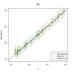
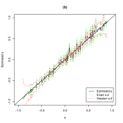
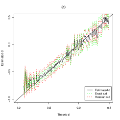
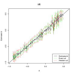
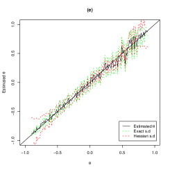
Figure 1: Dispersion plots between estimated and theoretical parameters of (a): ARFIMA$(0,d,0)$, (b)-(c): ARFIMA$(1,d,0)$ and (d)-(e): ARFIMA$(0,d,1)$ where the green dotted line is the exact standard deviation and the red line is the Hessian standard deviation.

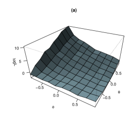
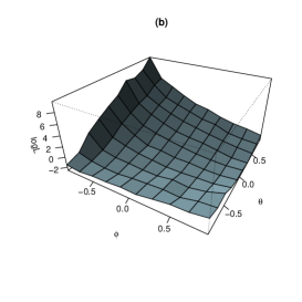
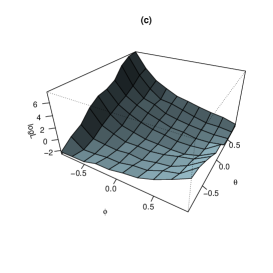
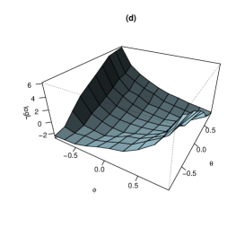
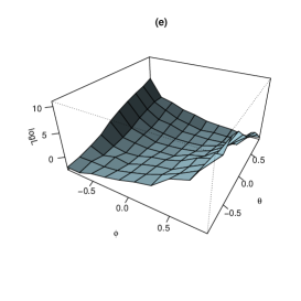
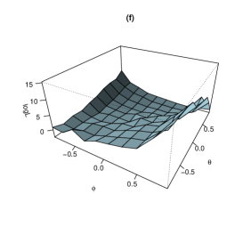
Figure 2: Log-Likelihood 3D plots for ARFIMA$(1,d,1)$ model with parameters (a) $d=-0\mbox{.}9$, (b) $d=-0\mbox{.}6$, (c) $d=-0\mbox{.}3$, (d) $d=0$, (e) $d=0\mbox{.}25$ and (f) $d=0\mbox{.}45$ using a grid $\phi\times\theta=(-0\mbox{.}9,0\mbox{.}9)\times(-0\mbox{.}9,0\mbox{.}9)$.

Figure 1 shows several simulation results assessing the performance of the estimators of $d$, AR, and the MA parameters, for different ARFIMA models. These plots include the exact and Hessian standard deviations. According to the definition of the ARFIMA model, the simulations are run in the interval $(-1,0\mbox{.}5)$ for $d$. In addition, Figure 2 shows some simulation results regarding the log-likelihood behavior for the cases $d=\{-0\mbox{.}9,-0\mbox{.}6,-0\mbox{.}3,0,0\mbox{.}25,0\mbox{.}45\}$ with a rectangular grid $\phi\times\theta=(-0\mbox{.}9,0\mbox{.}9)\times(-0\mbox{.}9,0\mbox{.}9)$ for the ARFIMA$(1,d,1)$ model. The plots of Figure 1 show a similar behavior for the estimators with respect to the theoretical parameters, except for the extreme values of the ARMA parameters near -1 and 1. Consequently, the confidence intervals tend to be larger than the other values of $\phi$ and $\theta$ parameters for plots (b) and (e). In addition, the plots of Figure 2 present low values of the likelihood function for the values of $\phi$ and $\theta$ closed to 0, especially for the plots (c)-(f) when $d=\{-0\mbox{.}3,0,0\mbox{.}25,0\mbox{.}45\}$. However, the plots (a)-(d) show high values of the likelihood function when this is evaluated for the points near $\phi=-0\mbox{.}9$ and $\theta=0\mbox{.}9$. For the plots (e)-(f), the behavior is inverse, i.e., the likelihood function tends to be higher for values near $\phi=0\mbox{.}9$ and $\theta=-0\mbox{.}9$.

2.2 Parameter variance-covariance matrix

Here, we discuss a method for calculating the exact asymptotic variance-covariance matrix of the parameter estimates. This is a useful tool for making statistical inferences about exact and approximate maximum likelihood estimators, such as the Haslett and Raftery (1989) and Whittle methods (see Section 2.1). An example of this calculation for an ARFIMA$(1,d,1)$ model is given by Palma (2007, pp. 105-108). This calculation method of the Fisher information matrix is an alternative to the numerical computation using the Hessian matrix.

This proposed method is based on the explicit formula obtained by means of the derivatives of the parameters log-likelihood gradients. From the spectral density defined in (6), we define the partial derivatives $\nabla_{\Phi}=(\partial/\partial\phi_{i})$ and $\nabla_{\Theta}=(\partial/\partial\theta_{j})$, with $i=1,\ldots,p$ and $j=1,\ldots,q$.

Theorem 2.2

Under the assumptions that $y_{t}$ is a stationary Gaussian sequence, the densities $f(\lambda)$, $f^{-1}(\lambda)$, $\partial/\partial{\bf\mu}_{i}f^{-1}(\lambda)$, $\partial^{2}/\partial{\bf\mu}_{i}\partial{\bf\mu}_{j}f^{-1}(\lambda)$ and $\partial^{3}/\partial{\bf\mu}_{i}\partial{\bf\mu}_{j}\partial{\bf\mu}_{k}f^{-1}(\lambda)$ are continuous in $(\lambda,{\bf\mu})$ for a parameter set ${\bf\mu}=\{d,\phi_{1},\ldots,\phi_{p},\theta_{1},\ldots,\theta_{q}\}$; we have the convergence in distribution for an estimated parameter $\widehat{\bf\mu}$ and the true parameter $\mu_{0}$ about a Gaussian ARFIMA model with

$$\sqrt{n}(\widehat{\bf\mu}_{n}-{\bf\mu}_{0})\mbox{ }\mathop{\buildrel d\over{\longrightarrow}}\limits_{n\rightarrow\infty}\mbox{ }N(0,{\bf\Sigma}^{-1}({\bf\mu}_{0})),$$ (12)

where

$${\bf\Sigma}({\bf\mu})=\frac{1}{4\pi}\int_{-\pi}^{\pi}[\nabla\hbox{log}f_{\bf\mu}(\lambda)][\nabla\hbox{log}f_{\bf\mu}(\lambda)]^{\top}d\lambda.$$ (13)

For a proof of Theorem 2.2, see e.g. Palma (2007). Thus, if we consider the model (1) with spectral density (6) where $\{\varepsilon_{t}\}$ is an independent and identically distributed $N(0,\sigma^{2})$, we have that the parameter variance-covariance matrix $\Gamma$ may be calculated in the following proposition.

Proposition 2.3

If $\{y_{t}\}$ is stationary, then

$$\frac{\partial}{\partial d}\hbox{log}f(\lambda) = -\hbox{log}[2(1-\cos\lambda)],$$

$$\frac{\partial}{\partial\phi_{\ell}}\hbox{log}f(\lambda) = \frac{\sum_{j=1}^{p}\phi_{j}\cos[(\ell-j)\lambda]}{\sum_{j=1}^{p}\sum_{k=1}^{p}\phi_{j}\phi_{k}\cos[(j-k)\lambda]},$$

$$\frac{\partial}{\partial\theta_{\ell}}\hbox{log}f(\lambda) = \frac{\sum_{j=1}^{q}\theta_{j}\cos[(\ell-j)\lambda]}{\sum_{j=1}^{q}\sum_{k=1}^{q}\theta_{j}\theta_{k}\cos[(j-k)\lambda]}.$$

Proof

First, from the spectral density given in (6) we have that

$$\hbox{log}f(\lambda)=\hbox{log}\left(\frac{\sigma^{2}}{2\pi}\right)-d\hbox{log}[2(1-\cos\lambda)]+\hbox{log}|\Theta(e^{i\lambda})|^{2}-\hbox{log}|\Phi(e^{i\lambda})|^{2}.$$

By Theorems 2.1 and 2.2, we observe that $\Phi(e^{i\lambda})=\sum_{j=1}^{p}\phi_{j}e^{i\lambda j}$, this yields

$$|\Phi(e^{i\lambda})|^{2} = \sum_{j=1}^{p}\sum_{k=1}^{p}\phi_{j}\phi_{k}e^{i\lambda(j-k)}$$

$$= 2\sum_{j=1}^{p}\sum_{k=1}^{p}\phi_{j}\phi_{k}\cos[(j-k)\lambda],$$

and

$$\frac{\partial}{\partial\phi_{\ell}}|\Phi(e^{i\lambda})|^{2} = 2\phi_{\ell}+\sum_{j\neq\ell}\phi_{j}e^{i\lambda(\ell-j)}+\sum_{k\neq\ell}\phi_{k}e^{i\lambda(\ell-k)}$$

$$= \sum_{j=1}^{p}\phi_{j}e^{i\lambda(\ell-j)}+\sum_{k=1}^{p}\phi_{k}e^{i\lambda(\ell-k)}$$

$$= 2\sum_{j=1}^{p}\phi_{j}\cos[(\ell-j)\lambda].$$

Analogously, we have that

$$\frac{\partial}{\partial\theta_{\ell}}|\Theta(e^{i\lambda})|^{2}=2\sum_{j=1}^{q}\theta_{j}\cos[(\ell-j)\lambda].$$

Then, this implies the results for $\frac{\partial}{\partial\phi_{\ell}}\hbox{log}f(\lambda)$ and $\frac{\partial}{\partial\theta_{\ell}}\hbox{log}f(\lambda)$. For $\frac{\partial}{\partial d}\hbox{log}f(\lambda)$ is direct.

Some computations and implementation of this matrix are described in Section 3.2, associated with the parameters of several ARFIMA models, using the Whittle estimator.

2.3 Impulse response functions

The impulse response functions (IRF) is the most commonly used tool to evaluate the effect of shocks on time series. Among the several approximations to compute this, we consider the theory proposed by Hassler and Kokoszka (2010) to find the IRF of a process $\{y_{t}\}$ following an ARFIMA($p,d,q$) model. The properties of these approximations, depend on whether the series are assumed to be stationary according to Theorem 2.1. So, under the assumption that the roots of the polynomials $\Phi(B)$ and $\Theta(B)$ are outside the closed unit disk and $d\in(-1,1/2)$, the process $\{y_{t}\}$ is stationary, causal and invertible. In this case, we can write $y_{t}=\Psi(B)\varepsilon_{t}$ where $\Psi(B)$ represents the expansion of the MA$(\infty)$ coefficients denoted as $\psi_{j}$ with $j>1$. These coefficients satisfy the asymptotic relationship $\psi_{j}\sim[\Theta(1)j^{d-1}]/[\Phi(1)\Gamma(d)]$ as $j\rightarrow\infty$ (Kokoszka and Taqqu, 1995), $\Theta(1)=1+\sum_{i=1}^{q}\theta_{i}$, and $\Phi(1)=1-\sum_{i=1}^{p}\phi_{i}$. As a particular case, we have that the $\psi_{j}$ coefficients for an ARFIMA$(0,d,0)$ are given in closed form by the expression $\psi_{j}=\Gamma(j+d)/(\Gamma(j+1)\Gamma(d))$. Now, from (2) and the Wold expansion (5), the process (1) has the expansion $(1-B)^{-d}y_{t}=\sum_{j=0}^{\infty}\eta_{j}y_{t-j}=\sum_{j=0}^{\infty}R_{j}\varepsilon_{t-j}$, where $R_{j}$ is the so-called IRF and is given by

$$R_{j}=\sum_{i=0}^{j}\psi_{i}\eta_{j-i}.$$ (14)

The terms $\eta_{j}$ can be represented in recursive form using (3) as $\eta_{j}=\left(1+(d-1)/j\right)\eta_{j-1}$, for $j\geq 1$ and $\eta_{0}=1$. From the asymptotic expression given in (4) and assuming that $\sum_{j=0}^{\infty}\psi_{j}<\infty$, we have the following asymptotic representation

$$R_{j}\sim\frac{j^{d-1}}{\Gamma(d)}\sum_{i=0}^{\infty}\psi_{i}$$ (15)

as $j\rightarrow\infty$ and $\psi_{j}/(j^{d-1})\longrightarrow 0$.

2.4 Autocovariance function

We illustrate a method to compute the exact autocovariance function for the general ARFIMA$(p,d,q)$ process. Considering the parameterization of the autocovariance function derived by writing the spectral density (6) in terms of parameters of the model given by Sowell (1992), the autocovariance function of a general ARFIMA$(p,d,q)$ process is given by

$$\gamma(h)=\frac{1}{2\pi}\int_{0}^{2\pi}f(\lambda)e^{-i\lambda h}d\lambda,$$ (16)

where $i$ denotes the imaginary unit. Particularly, the autocovariance and autocorrelation functions of the fractionally differenced ARFIMA$(0,d,0)$ process are given by

$$\gamma_{0}(h) = \sigma^{2}\frac{\Gamma(1-2d)}{\Gamma(1-d)\Gamma(d)}\frac{\Gamma(h+d)}{\Gamma(1+h-d)},$$

$$\rho_{0}(h) = \frac{\Gamma(1-d)}{\Gamma(d)}\frac{\Gamma(h+d)}{\Gamma(1+h-d)},$$

respectively. Then, the polynomial $\Phi(B)$ in (1) may be written as

$$\Phi(B)=\prod_{i=1}^{p}(1-\rho_{i}B).$$ (17)

Under the assumption that all the roots of $\phi(B)$ have multiplicity one, it can be deduced from (16) that

$$\gamma(h)=\sigma^{2}\sum_{i=-q}^{q}\sum_{j=1}^{p}\psi(i)\xi_{j}C(d,p+i-h,\rho_{j}).$$

with

$$\xi_{j} = \left[\rho_{j}\prod_{i=1}^{p}(1-\rho_{i}\rho_{j})\prod_{k\neq j}(\rho_{j}-\rho_{k})\right]^{-1},$$

$$C(d,h,\rho) = \frac{\gamma_{0}(h)}{\sigma^{2}}[\rho^{2p}\beta(h)+\beta(-h)-1],$$

$$\beta(h) = F(d+h,1,1-d+h,\rho),$$

$$F(a,b,c,x) = 1+\frac{a\cdot b}{c\cdot 1}x+\frac{a\cdot(a+1)\cdot b\cdot(b+1)}{c\cdot(c+1)\cdot 1\cdot 2}x^{2}+\ldots$$

where $F(a,b,c,x)$ is the Gaussian hypergeometric function (e.g. Gradshteyn and Ryzhik, 2007). The term $\psi(i)$ presented here and in Palma (2007, pp. 47-48) is a corrected version with respect to Sowell (1992) and is

$$\psi(i)=\sum_{k=\max(0,i)}^{\min(q,q+i)}\theta_{k}\theta_{k-i}.$$

In the absence of AR parameters the formula for $\gamma(h)$ reduces to

$$\gamma(h)=\sigma^{2}\sum_{i=-q}^{q}\psi(i)\frac{\Gamma(1-2d)\Gamma(h+d-i)}{\Gamma(1-d)\Gamma(d)\Gamma(1+i-d-h)}.$$

On the other hand, the findings of Hassler and Kokoszka (2010) describe the asymptotic behavior of the autocovariance function $\gamma(h)$ as

$$\gamma(h)\sim c_{\gamma}|h|^{2d-1},$$ (18)

where $c_{\gamma}=\sigma^{2}\pi^{-1}\Gamma(1-2d)\sin(\pi d)\left(\sum_{j=0}^{\infty}\psi_{j}\right)^{2}$ for large $|h|$. Let $\{y_{1},y_{2},\ldots,y_{n}\}$ be a sample from the process in (1) and let $\overline{y}$ be the sample mean. The exact variance of $\overline{y}$ is given by

$$\mbox{Var}(\overline{y})=\frac{1}{n}\left[2\sum_{j=1}^{n-1}\left(1-\frac{j}{n}\right)\gamma(j)+\gamma(0)\right].$$

By (18) and for large $n$, we have the asymptotic variance formula $\mbox{Var}(\overline{y})\sim n^{2d-1}c_{\gamma}/d(2d+1)$. The Sowell method is implemented in Section 3.3 for a selected ARFIMA$(1,d,1)$ model and its exact autocorrelation function is compared with the sample autocorrelation.

2.5 Predictive ability test

One approach to compare prediction models is through their root mean square error (RMSE). Under this paradigm and given two forecasting methods, the one that presents the lower RMSE is the better of the two. To compare statistically the differences of predictive ability among two proposed models, we focus here on the evaluation paradigm proposed by Giacomini and White (2006, GW). This test aims to evaluate a prediction method but not to carry out a diagnostic analysis. Therefore, it does not consider the parametric uncertainty, which is useful if we want to compare nested models from an ARFIMA model. The GW test attributed to Diebold and Mariano (1995) is based on the differences $\Delta L_{i}=|\widehat{x}_{i}-y_{i}|-|\widehat{z}_{i}-y_{i}|$, where $\widehat{x}_{i}$ and $\widehat{z}_{i}$ are the forecasted observations of the first and second model respectively, for $i=1,...,n$. The null hypothesis for the GW test associated with expected difference $E[\Delta L]$ of the two prediction models is $H_{0}$: $E[\Delta L]=0$, whereas the alternative is $H_{1}$: $E[\Delta L]\neq 0$. These hypotheses are tested by means of the statistic,

$$\Delta\widehat{L}(N)=\frac{1}{N\sqrt{\frac{\widehat{\sigma}^{2}_{N}}{N}}}\sum_{i=t_{0}}^{n-\tau}\Delta L_{i},$$

where $N=n-\tau-t_{0}+1$, $n$ is the total size of the sample, $\tau$ is the prediction horizon, and $t_{0}$ is the observation at which the mobile windows start. Note that under $H_{0}$, the statistic $\Delta\widehat{L}(N)$ is asymptotically normal. For $\tau=1$, an estimator of $\widehat{\sigma}_{N}$ can be obtained from the estimation of $\widehat{\sigma}_{\widehat{\alpha}}$ from a simple regression $\Delta\widehat{L}(N)=\widehat{\alpha}+\epsilon$. However, for horizons $\tau>1$, it is possible to apply a heteroscedasticity and autocorrelation consistent (HAC) estimator; for example, Newey and West (1987) or Andrews (1974). The GW test is implemented in the gw.test() function and described in Section 3.4.

3 Application

The functions described in the previous sections are implemented in the afmtools package. We illustrate the performance of the Whittle method by applications to real-life time series TreeRing (Statlib Data Base, http://lib.stat.cmu.edu/) displayed in Figure 3 left. In climatological areas, it is very important to analyze this kind of data because this allows us to explore rainy and dry seasons in the study area. Hipel and McLeod (1994) has been modeling this time series to determine the range of possible growths for the upcoming years of the trees using ARMA and ARIMA models. On the other hand, this time series displays a high persistence in its observations and has been analyzed by Palma and Olea (2010) and Palma et al. (2011) with a locally stationary approach. Apparently, the illustrated growth of the trees, represented by the number of the rings, presents a long-range dependence of its observations along the observations for ages and seasons (see Figure 3, right). For these reasons, we model the Tree Ring widths time series using long-memory models; specifically, the ARFIMA models are used to estimate, diagnose, and compare forecasts of the number of tree rings for upcoming years.

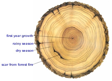
Figure 3: Left: Tree Ring Data Base. Right: Illustration of the observed climatic episodes and tree ring growth. Image source: http://summitcountyvoice.com

In order to illustrate the usage of package functions, we consider a fitted ARFIMA$(1,d,1)$ model. For this model, we have implemented the Whittle algorithm and computed the exact variance-covariance matrix to compare with the Hessian method. Afterward, we compare the Sowell method for computing the ACVF function with the sample ACVF. Other functions have also been implemented and illustrated in this section.

3.1 The implementation of the Whittle algorithm

The estimation of the fractionally, autoregressive, and moving-average parameters has been studied by several authors (Beran (1994); Haslett and Raftery (1989); Hyndman and Khandakar (2008)). A widely used method is the approximate MLE method of Haslett and Raftery (1989). In our study, estimation of the ARFIMA$(p,d,q)$ model using the corresponding Whittle method (Whittle, 1951) is described in Section 2.1 and this model is fitted by using the arfima.whittle function. To apply the Whittle algorithm to the TreeRing time series as an example, we use the following command considering an ARFIMA$(1,d,1)$ model.

R> y <- data(TreeRing)
R> model <- arfima.whittle(series = y, nar = 1, nma = 1, fixed = NA)

Note that the option fixed (for fixing parameters to a constant value) has been implemented. This option allows the user to fix the parameters $d$, $\phi_{1}$, or $\theta_{1}$, in order of occurrence. For example, in our ARFIMA$(1,d,1)$ model, we can set the parameter $d$ to be equal to zero. Consequently, we obtain the estimation of a simple ARMA$(1,1)$ model. The object model is of class arfima and provides the following features:

• estimation of $d$ and ARMA parameters;

• standard deviation errors obtained by the Hessian method and the respective t value and Pr(>|t|) terms;

• the log-likelihood function performed in the arfima.whittle.loglik() function;

• innovation standard deviation estimated by the ratio of the theoretical spectrum;

• residuals from the fitted model.

The commands plot(), residuals(), summary(), tsdiag() and print() have been adapted to this model class of S3 method. The summary() option shows the estimated parameters, the Hessian standard deviations, the $t$-statistic, and their respectively $p$-values. The computation of the long-memory parameter $d$ as well as the autoregressive $\{\phi_{1},...,\phi_{p}\}$ and moving average $\{\theta_{1},...,\theta_{q}\}$ parameters can be handled quickly for moderate sample sizes. Printing the model object by the summary() function shows the items mentioned before as

R> summary(model)
$call
arfima.whittle(series = y, nar = 1, nma = 1)

$coefmat
          Estimate  Std. Error   t value   Pr(>|t|)
d        0.1058021  0.04813552  2.198004 0.02794879
phi 1    0.3965915  0.03477914 11.403142 0.00000000
theta 1 -0.2848590  0.03189745 -8.930462 0.00000000

$sd.innov
[1] 35.07299

$method
[1] "Whittle"

attr(,"class")
[1] "summary.arfima"

Furthermore, we evaluate the Whittle estimation method for long-memory models by using the theoretical parameters versus the estimated parameters (see Figure 1). In addition, we compare the exact standards deviations of the parameters from Section 2.2 with those obtained by the Hessian method. These results and the evaluation of the Whittle estimations are illustrated in Table 1.

Table 1: Summary of estimated parameters for several ARFIMA models.

	FN$(d)$			ARFIMA$(1,d,0)$			ARFIMA$(0,d,1)$			ARFIMA$(1,d,1)$
Par.	Est	Hessian	Exact	Est	Hessian	Exact	Est	Hessian	Exact	Est	Hessian	Exact
$d$	0.195	0.048	0.023	0.146	0.048	0.038	0.156	0.048	0.035	0.106	0.048	0.063
$\phi$	-	-	-	0.072	0.029	0.049	-	-	-	0.397	0.035	0.282
$\theta$	-	-	-	-	-	-	0.059	0.029	0.045	-0.285	0.032	0.254

3.2 The implementation of exact variance-covariance matrix

The var.afm() function shows the exact variance-covariance matrix and the standard deviations. The computation of the integrals of the expression (13) is carried out by using the Quadpack numeric integration method (Piessens et al., 1983) implemented in the integrate() function (stats package). Note that the functions involved in these integrals diverge in the interval $\lambda=[-\pi,\pi]$. However, they are even functions with respect to $\lambda$. Thus, we integrate over $[0,\pi]$ and then multiply the result by two. Now, by using the central limit theorem discussed in Section 2.2, we can obtain the asymptotic approximation of the estimated parameters standards errors $\mbox{SE}(\widehat{{\bf\Omega}})_{i}=(\frac{1}{n}[\widehat{{\bf\Sigma}}^{-1}]_{ii})^{1/2}$ of an ARFIMA model, where $\widehat{{\bf\Omega}}=(\widehat{d},\widehat{\phi}_{1},\ldots,\widehat{\phi}_{p},\widehat{\theta}_{1},\ldots,\widehat{\theta}_{q})$ and $[\widehat{{\bf\Sigma}}^{-1}]_{ii}$ corresponds to the $i$th diagonal components of the matrix $\widehat{{\bf\Sigma}}^{-1}$ for $i=\{1,...,p+q+1\}$.

Table 2: Akaike’s criterion for $\widehat{{\bf\Omega}}=(\widehat{d},\widehat{\phi}_{1},\widehat{\phi}_{2},\widehat{\theta}_{1},\widehat{\theta}_{2})$ with $p$-values obtained for the Hessian standard deviation.

$p$	$q$	AIC	$\widehat{d}$	p-value
0	0	-37.018	0.196	0
0	1	-35.008	0.156	0.001
0	2	-33.000	0.113	0.018
1	0	-35.007	0.146	0.002
1	1	-33.004	0.106	0.028
1	2	-30.996	0.142	0.003
2	0	-33.002	0.111	0.021
2	1	-30.995	0.130	0.007
2	2	-28.915	0.191	0

By using the Whittle estimators, we search for the lowest AIC (Akaike Information Criterion, Akaike, 1974) given by $\mbox{AIC}(\widehat{\omega})=-2[\hbox{log}\,L(\widehat{\omega})-(p+q+1)]$ over a class of ARFIMA models with $p,q\in\{0,1,2\}$, where $\widehat{\omega}$ is a subset of $\widehat{{\bf\Omega}}$ and $L(\widehat{\omega})$ is the likelihood associated with $\widehat{\omega}$. From Table 2, we can see that the fractionally differenced model ARFIMA($0,d,0$) has the lowest AIC. Candidate models are marked in bold in Table 2.

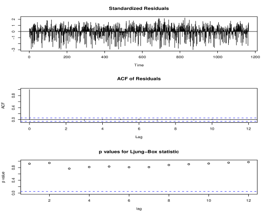
Figure 4: Plots of residuals analysis from tsdiag standard command adapted to ARFIMA model residuals.

Additionally, we propose a technique for obtaining the spectral density associated with ARFIMA and ARMA processes in spectrum.arfima() and spectrum.arma(), respectively. This is done by using the polyroot() function of the polynom package to compute the roots of the polynomials $\Phi(e^{-i\lambda})$ and $\Theta(e^{-i\lambda})$. Both functions need the estimated ARFIMA parameters and the sd.innov innovation standard estimation given by an object of arfima class. For the spectrum density and periodogram, see Section 2 and Subsection 2.1, respectively. Since the calculation of the FFT has a numerical complexity of the order $O[n\hbox{log}_{2}(n)]$, this approach produces a very fast algorithm to estimate the parameters. It is possible to obtain the FFT through the fft() function based on the method proposed by Singleton (1979).

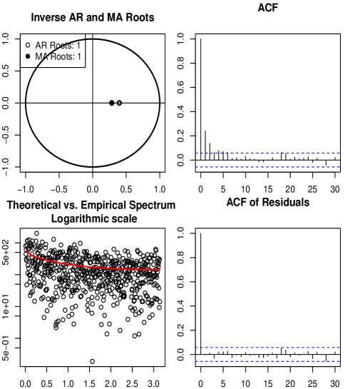
Figure 5: Diagnostic Plots made by the plot() command. Left: Plots of unit roots circle along with the root provided by AR and MA polynomials and Theoretical (red line) vs. Empirical Spectrum (back points) plot. Right: ACF plots of Tree Rings and ARFIMA$(1,d,1)$ model residuals.

3.3 The implementation of the diagnostic functions

We have also implemented a very practical function called check.parameters.arfima(). This verifies whether the long-memory parameter $d$ belongs to the interval $(-1,0\mbox{.}5)$ and whether the roots of the fitted ARMA parameters lie outside the unit disk. This function was incorporated in the plot() command. In the first plot of Figure 5, we can see that the roots of the AR and MA polynomials lie outside the unit disk, according to the assumptions of stationarity solutions of (1) presented in Theorem 2.1 (see Section 2). Alternatively, the check.parameters.arfima() that takes an arfima-class object, gives TRUE/FALSE-type results indicating whether the parameters pass the requirement for a stationary process.

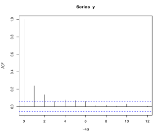
Figure 6: Theoretical (left) and Empirical (right) ACF of selected ARFIMA model.

Figure 7: Plots of IRFs methods for $h=50$, 100 and 150 lags.

Additionally, an adaptation of the function tsdiag() can be found in this package. This is implemented in an S3-type arfima class method and shows three plots for analyzing the behavior of the residual from the fitted ARFIMA model. This function has additional arguments such as the number of observations n for the standardized residuals and critical $p$-value alpha. Figure 4 illustrates these results, where, the residuals are white noise at a confidence level of $\alpha=95\%$.

On the other hand, the $R_{j}$ (IRF) illustrated in Figure 7 decays exponentially fast, at a rate of $j^{d-1}$ because, these functions inherit the behavior of $\eta_{j}$. This behavior is typical for ARFIMA models, as reported by Hassler and Kokoszka (2010), Kokoszka and Taqqu (1995) and Hosking (1981). Figure 7 shows some $R_{j}$ curves associated with the three models considered in Table 1 for the asymptotic method by formula (15) (labeled Asymptotic in the plot) and the counterpart method by formula (14) (labeled Normal in the plot). Note that for a large value of $j\approx 50$, both methods tend to converge, and, the curves make an inflexion in the value $j\approx 10$. Note that the Asymptotic approximation tends to be equal to the Normal method in the measure that the input h lag increases (see plots for h=150 in Figure 7). These IRFs are available in the function ir.arfima(), with arguments h to evaluate the IRFs over a particular $h$ lag and, model for an object arfima.whittle. The ir.arfima() function produces the vectors RE and RA for Normal and Asymptotic IRFs.

The exact Sowell autocovariance computation obtained by rho.sowell() and the sample autocorrelation obtained by the ACF() command are applied to tree ring time series. In Figure 6, the blue dotted lines in the first plot correspond to the $\{\mp 2/\sqrt{n}\}$ significance level for the autocorrelations. The function rho.sowell() requires the specification of an object of class arfima in the object option that, by default, is NULL. But, if object=NULL, the user can incorporate the ARFIMA parameters and the innovation standard deviation. Alternatively, the implemented plot option gives a graphical result similar to the ACF() command in the sample autocorrelation. We can see the similarity of both results for the discussed model. The ACVF implementation is immediate but, for the calculation of the Gaussian hypergeometric functions, we use the hypergeo() function from the hypergeo package. For values of $h>50$, we use the approximation (18) reducing considerably the computation time as compared to the Sowell algorithm.

On the other hand, the rho.sowell() function is required by the function smv.afm(). The function smv.afm() calculates the variance of the sample mean of an ARFIMA process. When the argument comp is TRUE, the finite sample variance is calculated, and when comp is FALSE, the asymptotic variance is calculated.

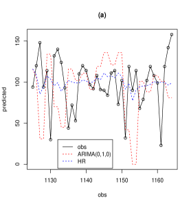
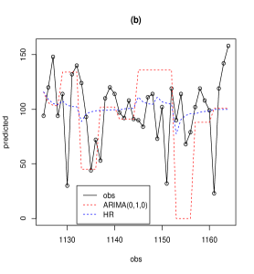
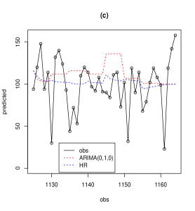
Figure 8: Plots of out-of-sample predictions for (a) $\tau=2$, (b) $\tau=4$ and (c) $\tau=5$ for two models: ARIMA(0,1,0) in red and ARFIMA$(1,d,1)$ in blue with Haslett & Raftery estimator (HR).

Table 3: Summary of p-values of the GW test for each HAC estimator, $\tau=\{2,4,5\}$ prediction horizon parameters and for the estimator methods B (Benchmark model), ML (ARFIMA models using Maximum Likelihood estimator) and HR (ARFIMA models using Haslett & Raftery estimator) over 40 observations of samples from the TreeRing data set. The $p$-values marked in bold are lower than the probability (0.05) related to a 5% confidence level.

HAC	Prediction Horizon Parameter
Estimators	$\tau=2$				$\tau=4$				$\tau=5$
		$B$	$ML$	$HR$		$B$	$ML$	$HR$		$B$	$ML$	$HR$
	$B$	-	0.001	0.001	$B$	-	0.031	0.031	$B$	-	0.126	0.126
HAC	$ML$	0.001	-	0.307	$ML$	0.031	-	0.559	$ML$	0.126	-	0.689
	$HR$	0.001	0.307	-	$HR$	0.031	0.559	-	$HR$	0.126	0.689	-
		$B$	$ML$	$HR$		$B$	$ML$	$HR$		$B$	$ML$	$HR$
Newey &	$B$	-	0.002	0.002	$B$	-	0.051	0.051	$B$	-	0.174	0.174
West	$ML$	0.002	-	0.005	$ML$	0.051	-	0.281	$ML$	0.174	-	0.479
	$HR$	0.002	0.005	-	$HR$	0.051	0.281	-	$HR$	0.174	0.479	-
		$B$	$ML$	$HR$		$B$	$ML$	$HR$		$B$	$ML$	$HR$
Lumley &	$B$	-	0.001	0.001	$B$	-	0.023	0.023	$B$	-	0.096	0.096
Heagerty	$ML$	0.001	-	0.486	$ML$	0.023	-	0.652	$ML$	0.096	-	0.762
	$HR$	0.001	0.486	-	$HR$	0.023	0.652	-	$HR$	0.096	0.762	-
		$B$	$ML$	$HR$		$B$	$ML$	$HR$		$B$	$ML$	$HR$
	$B$	-	0.003	0.003	$B$	-	0.041	0.041	$B$	-	0.206	0.206
Andrews	$ML$	0.003	-	0.018	$ML$	0.041	-	0.283	$ML$	0.206	-	0.456
	$HR$	0.003	0.018	-	$HR$	0.041	0.283	-	$HR$	0.206	0.456	-

3.4 Forecasting evaluations

The GW method implemented in gw.test() for evaluating forecasts proposed by Giacomini and White (2006) compares two vectors of predictions, x and y, provided by two time series models and a data set p. We consider that it is relevant to implement this test to determine if the predictions produced by a time series model (e.g., ARFIMA) process good forecasting qualities. This test for predictive ability is of particular interest since it considers the tau prediction horizon parameter or ahead in the case of pred.arfima() function. Alternative methods are discussed, for instance, by Diebold and Mariano (1995). If tau=1, the standard statistic simple regression estimator method is used. Otherwise, for values of tau larger than 1, the method chosen by the user is used in the method option. The available methods for selection are described below. They include several Matrix Covariance Estimation methods but, by default, the HAC estimator is used in the test. The user can select between the several estimators of the sandwich package mentioned before:

• HAC: Heteroscedasticity and Autocorrelation Consistent (HAC) Covariance Matrix Estimation by vcovHAC() function (Zeileis (2004); Zeileis (2006)).

• NeweyWest: Newey-West HAC Covariance Matrix Estimation by NeweyWest() function (Newey and West (1987)).

• LumleyHeagerty: Weighted Empirical Adaptive Variance Estimation by weave() function (Lumley and Heagerty (1999)).

• Andrews: Kernel-based HAC Covariance Matrix Estimation by kernHAC() function (Andrews (1974); Andrews and Monahan (1992)).

This test gives the usual results of the general test implemented in such as the GW statistic in statistic, the alternative hypothesis in alternative, the $p$-value in p.value, others such as the method mentioned before in method, and the name of the data in data.name. In some studies, the GW test is used to compare selected models versus benchmark models such as ARMA, ARIMA, or SARIMA models (e.g. Contreras-Reyes and Idrovo, 2011). So, to illustrate the GW test performance, we simulate the out-of-sample prediction exercise through mobile windows for TreeRing data sets considering the first 1124 observations and, later, forecasting 40 observations using three models: the ARIMA(0,1,0) benchmark model, the ARFIMA$(p,d,q)$ with MLE estimator, and the Haslett & Raftery estimator (HR) using the algorithm of the automatic forecast() function implemented in the forecast package by Hyndman and Khandakar (2008) algorithm. In Figure 8, the GW test compares the out-of-sample predictions of the ARIMA(0,1,0) and ARFIMA(p,d,q) model. It is important to note that the goal of this test is only to compare prediction abilities between models.

Finally, we study a more general simulation, comparing the three predictors vectors with 40 real observations using gw.test() function considering the hypotheses testing alternative="two.sided" to contrast significant differences between predictions. In addition, we consider the four HAC estimators mentioned in the beginning of this subsection and prediction horizon parameters $\tau=\{2,4,5\}$. The results are summarized in Table 3 and Figure 8. We can see that the differences in the prediction ability between B vs. MLE and B vs. HR are significant for $\tau=2$ and 4 but, between MLE and HR they are not unequal for the three considered values of $\tau$. Given the non-significance of the MLE-HR test $p$-value, the MLE model is not considered in Figure 8. As expected, the increments of the prediction horizon parameter showed that the different prediction abilities of the models tend to be zero because the time series uncertainty tends to increase. Consequently, the individual prediction performance of each model is not considered by the test.

4 Conclusions

We developed the afmtools package with the goal of incrementing the necessary utilities to analyze the ARFIMA models and, consequently, it is possible to execute several useful commands already implemented in the long-memory packages. In addition, we have provided the theoretical results of the Whittle estimator, which were applied to the Tree Ring data base. Furthermore, we have performed a brief simulation study for evaluating the estimation method used herein and also have evaluated the properties of its log-likelihood function. The numerical examples shown here illustrate the different capabilities and features of the afmtools package; specifically, the estimation, diagnostic, and forecasting functions. The afmtools package would be improved by incorporating other functions related to change-point models and tests of unit roots, as well as other important features of the models related to long-memory time series.

Acknowledgment Wilfredo Palma would like to thank the support from Fondecyt Grant 1120758.

References

- Akaike (1974) Akaike, H. (1974). A new look at the statistical model identification. IEEE Trans. Automat. Control, 19, 6, 716-723.
- Andrews (1974) Andrews, D. (1991). Heteroskedasticity and Autocorrelation Consistent Covariance Matrix Estimation. Econometrica, 59, 3, 817-858.
- Andrews and Monahan (1992) Andrews, D., Monahan, J.C. (1992). An Improved Heteroskedasticity and Autocorrelation Consistent Covariance Matrix Estimator. Econometrica, 60, 4, 953-966.
- Beran (1994) Beran, J. (1994). Statistics for Long-Memory Processes, Chapman & Hall, New York.
- Bisaglia and Guégan (1998) Bisaglia, L., Guégan, D. (1998). A comparison of techniques of estimation in long-memory processes. Comput. Stat. Data An., 27, 61-81.
- Contreras-Reyes et al. (2011) Contreras-Reyes, J.E., Goerg, G., Palma, W. (2011). Estimation, Diagnostic and Forecasting Functions for ARFIMA models. R package version 0.1.7, http://cran.r-project.org/web/packages/afmtools/index.html.
- Contreras-Reyes and Idrovo (2011) Contreras-Reyes, J., Idrovo, B. (2011). En busca de un modelo Benchmark Univariado para predecir la tasa de desempleo de Chile. Cuadernos de Economía, 30, 55, 105-125.
- Dahlhaus (1994) Dahlhaus, R. (1994). Efficient parameter estimation for self-similar processes. Ann. Stat., 17, 4, 1749-1766.
- Diebold and Mariano (1995) Diebold, F., Mariano, R. (1995). Comparing Predictive Accuracy. J. Bus. Econ. Stat., 13, 3, 253-263.
- Giacomini and White (2006) Giacomini, R., White, H. (2006). Tests of Conditional Predictive Ability. Econometrica, 74, 6, 1545-1578.
- Gradshteyn and Ryzhik (2007) Gradshteyn, I.S., Ryzhik, I.M. (2007). Table of Integrals, Series, and Products. Seventh Edition. Elsevier, Academic Press.
- Granger and Joyeux (1980) Granger, C.W., Joyeux, R. (1980). An introduction to long-memory time series models and fractional differencing. J. Time Ser. Anal., 1, 15-29.
- Haslett and Raftery (1989) Haslett J. & Raftery A. E. (1989). Space-time Modelling with Long-memory Dependence: Assessing Ireland’s Wind Power Resource (with Discussion). Appl. Stat., 38, 1, 1-50.
- Hassler and Kokoszka (2010) Hassler, U., Kokoszka, P.S. (2010). Impulse Responses of Fractionally Integrated Processes with Long Memory. Economet. Theor., 26, 6, 1885-1861.
- Hipel and McLeod (1994) Hipel, K.W., McLeod, A.I. (1994). Time Series Modelling of Water Resources and Environmental Systems, Elsevier Science, The Netherlands.
- Hosking (1981) Hosking, J.R. (1981). Fractional differencing. Biometrika, 68, 1, 165-176.
- Hyndman and Khandakar (2008) Hyndman, R.J., Khandakar, Y. (2008). Automatic Time Series Forecasting: The forecast Package for R. J. Stat. Softw., 27, 3, 1-22.
- Kokoszka and Taqqu (1995) Kokoszka, P.S., Taqqu, M.S. (1995). Fractional ARIMA with stable innovations. Stoch. Proc. Appl., 60, 1, 19-47.
- Lumley and Heagerty (1999) Lumley, A., Heagerty, P. (1999). Weighted Empirical Adaptive Variance Estimators for Correlated Data Regression. J. Roy. Stat. Soc. B Met., 61, 2, 459-477.
- Newey and West (1987) Newey, W.K., West, K.D. (1987). A Simple, Positive Semidefinite, Heteroskedasticity and Autocorrelation Consistent Covariance Matrix. Econometrica, 55, 3, 703-708.
- Palma (2007) Palma, W. (2007). Long-Memory Time Series, Theory and Methods. Wiley-Interscience. John Wiley & Sons.
- Palma and Olea (2010) Palma, W., Olea, R. (2010). An efficient estimator for locally stationary Gaussian long-memory processes. Ann. Stat., 38, 5, 2958-2997.
- Palma et al. (2011) Palma, W., Olea, R., Ferreira, G. (2011). Estimation and Forecasting of Locally Stationary Processes. J. Forecast., DOI: 10.1002/for.1259.
- Peiris and Perera (1988) Peiris, M., Perera, B. (1988). On prediction with fractionally differenced ARIMA models. J. Time Ser. Anal., 9, 3, 215-220.
- Piessens et al. (1983) Piessens, R., de Doncker-Kapenga, E., Uberhuber, C., Kahaner, D. (1983). Quadpack: a Subroutine Package for Automatic Integration, Springer-Verlag, New York.
- R Development Core Team (2012) R Development Core Team (2012). R: A Language and Environment for Statistical Computing. Foundation for Statistical Computing, Vienna, Austria. ISBN 3-900051-07-0, http://www.R-project.org.
- Singleton (1979) Singleton, R.C. (1979). Mixed Radix Fast Fourier Transforms, in Programs for Digital Signal Processing. IEEE Digital Signal Processing Committee eds. IEEE Press.
- Sowell (1992) Sowell, F. (1992). Maximum likelihood estimation of stationary univariate fractionally integrated time series models. J. Econometrics, 53, 1-3, 165-188.
- Whittle (1951) Whittle P. (1951). Hypothesis Testing in Time Series Analysis. Hafner, New York.
- Wold (1938) Wold, H. (1938). A Study in the Analysis of Stationary Time Series. Almqvist and Wiksell, Uppsala, 53, 165-188.
- Zeileis (2004) Zeileis, A. (2004). Econometric Computing with HC and HAC Covariance Matrix Estimators. J. Stat. Softw., 11, 10, 1-17.
- Zeileis (2006) Zeileis, A. (2006). Object-oriented Computation of Sandwich Estimators. J. Stat. Softw., 16, 9, 1-16.