Block-Relaxation Methods for 3D Constant-Coefficient Stencils
on GPUs and Multicore CPUs

Abstract

Block iterative methods are extremely important as smoothers for multigrid methods, as preconditioners for Krylov methods, and as solvers for diagonally dominant linear systems. Developing robust and efficient smoother algorithms suitable for current and evolving GPU and multicore CPU systems is a significant challenge. We address this issue in the case of constant-coefficient stencils arising in the solution of elliptic partial differential equations on structured 3D uniform and adaptively refined grids. Robust, highly parallel implementations of block Jacobi and chaotic block Gauss-Seidel algorithms with exact inversion of the blocks are developed using different parallelization techniques. Experimental results for NVIDIA Fermi/Kepler GPUs and AMD multicore systems are presented.

1 Introduction

Iterative methods such as Jacobi, Gauss-Seidel, Successive Over-Relaxation (SOR), and their variants are extremely important as smoothers for multigrid methods [2, 3], preconditioners for Krylov methods [4], and as solvers for diagonally dominant linear systems. Their widespread use in iterative solution methods for linear systems has led to significant effort being devoted to optimizing their performance on modern GPU and multicore systems. Much of the attention has been focused on point-wise versions of these methods to exploit parallelism [5].

However, block versions of these methods, in particular line and plane smoothers, are extremely important as key components of robust geometric multigrid methods [6, 7] and multilevel iterative methods (such as the Fast Adaptive Composite-Grid (FAC) and Multi-Level Adaptive Technique (MLAT) methods [8, 9]) on adaptively refined grids. Early work by Shortley and Weller [10] and Parter [11] has shown that even for isotropic diffusion problems block Jacobi and Gauss-Seidel can have advantages. More recently, Philip and Chartier demonstrated how to automatically construct block iterative methods for fairly general linear systems based on algebraic measures of coupling [12]. Furthermore, block iterative methods have the potential to increase local computation and decrease communication on next generation parallel systems where communication increasingly dominates costs.

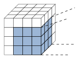
(a)

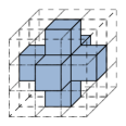
(b)

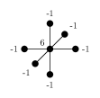
(c)

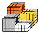
(d)

Figure 1: In Figure 1a a patch is shown with an extraction of cells (shaded). The 7-point stencil in Figure 1c arises from the shaded cells in Figure 1b. A domain composed of 4 patches is shown in Figure 1d.

In this context, recent work focused on GPU implementations includes the 2D block based smoother of Feng et al. [13] and the 1D block-asynchronous smoother for multigrid methods by Anzt et al. [14]. However, both works use Jacobi iterations within each block, rendering them closer to two-level Jacobi methods or Jacobi-Gauss-Seidel methods. These can be considered as variants on the work presented in Venkatasubramanian et al. [15]. Recent work in the context of multicore CPUs includes that by Adams et al. [16, 17] on block Gauss-Seidel algorithms.

In this paper we focus on developing efficient block-iterative Jacobi and chaotic Gauss-Seidel methods on current and evolving GPU and multicore architectures. We will demonstrate simple, efficient and general block smoothing algorithms with exact inversion of the blocks for 3D constant-coefficient elliptic problems. Such problems are of importance in a wide variety of scientific computations. We will consider only single node GPU and multicore algorithms in this paper with future work extending the results of this paper to distributed systems. The processing power and memory capacity of single node systems enable fairly large simulations particularly when Adaptive Mesh Refinement (AMR) is used where the memory and compute requirements drop significantly (approximately 10% of uniform grid computations [19, 20] in our experience), making the results of this paper relevant in that context.

1.1 Model Problem

We will focus on the model problem for the 3D Poisson equation

$$-\nabla^{2}u\left(\mathbf{x}\right) = f(\mathbf{x}),\;\;\mathbf{x}\equiv\left(x,y,z\right)\in\Omega,$$

$$u\left(\mathbf{x}\right) = 0,\;\;\mathbf{x}\in\partial\Omega,$$ (1)

for simplicity, though the presented methods will be applicable to any constant-coefficient elliptic system such as the recent work by Guy et al. [18] on block smoothers for Stokes problems. Here $\nabla^{2}$ is the Laplacian operator, $f$ is a source and $u$ is the solution to Equation (1.1) on a cubic domain $\Omega\equiv\left[0,1\right]^{3}\subset\mathbb{R}^{3}$ with Dirichlet boundary conditions on the boundary $\partial\Omega$. We set $f\left(x\right)=0$ for simplicity because our focus is on the smoothing algorithm.

It is assumed that the reader is familiar with discretization methods and only a brief description is provided to establish notation. The methods presented are not tied to any particular discretization, though for concreteness we use a cell-centered finite volume (FVM) discretization with variable unknowns located at cell centers. FVM discretization methods for single logically rectangular domains begin by partitioning the continuous domain $\Omega$ into a set of discrete cells that together form a regular patch with $n_{x}$, $n_{y}$, and $n_{z}$ cells in the $x$-, $y$-, and $z$-directions respectively as in Figure 1a. Each cell volume is then uniquely indexed by a triple $(i,j,k)$ specifying location in space: $\left[i\cdot h_{x},\left(i+1\right)\cdot h_{x}\right]\times\left[j\cdot h_{y},\left(j+1\right)\cdot h_{y}\right]\times\left[k\cdot h_{z},\left(k+1\right)\cdot h_{z}\right]$ with $0\leq i\leq n_{x}-1$, $0\leq j\leq n_{y}-1$, $0\leq k\leq n_{z}-1$. Here $h_{x},h_{y},$ and $h_{z}$ represent the cell widths in each direction. To simplify notation going forward we assume $h_{x}=h_{y}=h_{z}=h$. A cell-centered finite-volume approximation of equation (1.1) then leads to the following system of equations for each cell:

$$6u_{i,j,k}-u_{i-1,j,k}-u_{i+1,j,k}-u_{i,j-1,k}$$

$$-u_{i,j+1,k}-u_{i,j,k-1}-u_{i,j,k+1}=h^{2}f_{i,j,k},$$ (2)

where $u_{i,j,k}$ represents an approximation to $u$ in cell $\left(i,j,k\right)$. Since the coefficients in Equation (1.1) have no spatial dependence a stencil representation as depicted in Figure 1c can be used to represent both the coefficient and connectivity information for each cell in a patch. Cells on patch boundaries have the same stencil as interior cells, since we assume that each patch has a layer of ‘ghost’ cells around it (Figure 2b) to which boundary conditions are extrapolated. The methodology outlined extends with minor modifications to discretizing a collection of non-overlapping logically rectangular patch domains as in Figure 1d. Interior ghost cells at patch interfaces are then used to ensure consistency across patches.

Many simulations of physical phenomena often need to resolve extremely fine-scale features localized in space and/or time [19, 20]. Discretizing the entire physical domain at the required fine-scale resolution is then often impractical and not necessary. Instead AMR can be used to increase the local resolution only where required. Given a collection of patches that cover the domain $\Omega_{1}\equiv\Omega$ at some coarse resolution $h_{1}=h$, structured AMR techniques identify a local subdomain $\Omega_{2}$ where finer resolution is required ($\Omega_{2}$ may consist of disjoint subdomains). A collection of patches with the same finer resolution $h_{2}$ are then introduced to cover $\Omega_{2}$. Together, they form a refinement level covering the subdomain $\Omega_{2}$. A typical choice of $h_{2}$ is $h_{1}/2$. Repeating this process leads to a set of increasingly finer nested refinement levels, each consisting of a collection of logically rectangular patches. Patches in this hierarchy are dynamically created and destroyed as the simulation progresses depending on local resolution requirements. Large-scale parallel structured AMR calculations can employ thousands of patches on each refinement level, with each processor owning multiple patches from potentially different refinement levels. Methods such as FAC [8] and MLAT [9] smooth on these patches during the solution process.

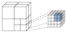
(a)

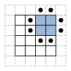
(b)

Figure 2: (a) Left: 3D AMR patch hierarchy with outlines of 8 patches on level 0 and 8 patches on level 1. Right: patch with shaded cells corresponding to a geometric block. (b) 2D patch slice with ghost and neighbor cells for a block (shaded).

For the purposes of block smoothing, patches in the refinement hierarchy are typically too large to be processed efficiently. Instead patches are decomposed into smaller geometric blocks. For example, Figure 2a shows a $2\times 2\times 2$ block (shaded) consisting of 8 cells in a $4\times 4\times 4$-cell patch. Thus, the patch of size $4^{3}$ cells in Figure 2a is decomposed into 8 blocks of size $2^{3}$. Stencil operations for each block in the patch have dependencies on neighbor and ghost cell data as shown in Figure 2b. As mentioned, the block relaxation methods we describe below are meant to be used as components of multigrid or multilevel methods consisting of multiple structured patches over a domain or a hierarchy of sub-domains in the case of AMR.

The remainder of the paper is organized as follows. Section 2 describes block-relaxation methods and algorithm choices based on GPU and multicore CPU architectures. Section 3 discusses different parallelization strategies and considerations in the choice of block sizes. We state experimental results using state-of-the-art hardware including the NVIDIA Kepler K20X GPU and a CRAY XE6 compute node in Section 4. The last section presents conclusions and an overview of possible future research directions.

2 Block Smoothing Algorithms

Discretizing equation (1.1) on a patch or a collection of patches leads to a linear system of equations, one equation per grid cell, of the form of equation (1.1). The resulting linear system of equations can be written in matrix form as

$$A\mathbf{u} = \mathbf{f}$$ (3)

with $A\in\mathbb{R}^{m\times m}$, and $\mathbf{u},\mathbf{f}\in\mathbb{R}^{m}$ with a suitable mapping from the matrix ordering to the $(i,j,k)$ ordering on patches. Let $A$ be partitioned into a set of submatrices as shown below.

$$A=\left[\begin{array}[]{cccc}A_{11}&A_{12}&\cdots&A_{1s}\\ A_{21}&A_{22}&\cdots&A_{2s}\\ \cdots&\cdots&\cdots&\cdots\\ A_{s1}&\cdots&A_{s,s-1}&A_{ss}\end{array}\right]$$ (8)

where $A_{ij},\,1\leq i,j\leq s$ are now $s^{2}$ matrix subblocks of size $q_{i}\times q_{j}$ with $\sum_{1}^{s}q_{i}=m$. The partitioning of $A$ into subblocks could be based on mapping to/from geometric blocks of a structured grid as described earlier or on other considerations such as anisotropic features in the PDE, or algebraic strength of coupling measures between variables. It is assumed that the diagonal blocks, $A_{ii},1\leq i\leq s$, are invertible. For the purposes of this paper it is sufficient to consider the matrix blocks as arising from a lexicographical ordering of geometric blocks within each patch. Furthermore, from this point on we will assume that all matrix blocks are of the same size. A block stationary iterative method can now be defined by a splitting, $A=M-N$, where $M$ is invertible, which leads to the stationary iteration

$$\mathbf{u}^{k+1}=M^{-1}N\mathbf{u}^{k}+M^{-1}\mathbf{f},$$ (9)

where $k$ is the iteration number. The iteration given above converges if and only if $\rho(M^{-1}N)<1$, where $\rho$ denotes the spectral radius operator. An equivalent formulation of (9) is:

$$\mathbf{u}^{k+1}=\mathbf{u}^{k}+M^{-1}\mathbf{r}^{k}$$ (10)

for residual $\mathbf{r}^{k}=\mathbf{f}-A\mathbf{u}^{k}$, which will be the form used in this paper. An example of a block iteration is the block Gauss-Seidel method defined by the splitting

$$M=\left[\begin{array}[]{cccc}A_{11}&0&\cdots&0\\ A_{21}&A_{22}&\cdots&0\\ \cdots&\cdots&\cdots&\cdots\\ A_{s1}&\cdots&A_{s,s-1}&A_{ss}\end{array}\right]$$ (15)

and $N=M-A$. When $s=m$, the subblocks are of size one and the iteration reduces to the standard lexicographic Gauss-Seidel iteration. A block Jacobi algorithm is obtained if $A_{ij}=0$ for $i>j$ also in equation (15). The numerical results presented in this paper were all performed with block (chaotic) Gauss-Seidel and damped block Jacobi iterations, though once the block partitioning is defined we are free to choose any suitable block-iterative process.

In general, it is difficult to provide theoretical results that guarantee that a given block-iterative method formed will converge or that a particular choice of blocks will lead to a faster rate of convergence as opposed to an alternative choice of blocks. The interested reader is referred to Varga [21] for theoretical results on general block iterative methods and to Parter [11] for some early work on block iterative methods for elliptic equations.

The block-smoothing iteration derived from Equation (10) employs a direct solve to compute the inverse $\hat{A}_{b}:=A_{ii}^{-1}$ for the diagonal block $A_{b}:=A_{ii}$ with $b,i=1,\ldots,s$. The cost of computing this inverse for a block, and restrictions that apply in the case that the patch size is not a multiple of the block size, are described in Section 4.3. There it will be shown that it is sufficient to assume that only one inversion is necessary for a patch and this inversion has already been performed before the smoothing iterations are executed.

Updating the neighbor cells of a spatial block as in Figure 2b can be performed in different ways. Our implementation of the block smoothing algorithm employs either a classic Jacobi update or a chaotic block Gauss-Seidel update scheme between the blocks. This chaotic relaxation was first proposed by Chazan and Miranker [22]. Some current research on chaotic relaxation using shared and distributed memory systems can be found under asynchronous iteration in [23, 24, 25]. Baudet [24] defines the term chaotic relaxation scheme to describe a purely or totally asynchronous method, which accurately describes our chaotic block Gauss-Seidel implementation. Bertsekas et al. state in [26] a general convergence theorem for totally asynchronous algorithms in the case of fixed-point problems. A modified convergence theorem based on Chazan and Miranker with constraints on global memory and communication is presented by Strikwerda [27]. Blathras et al. state a timing model and stopping criteria for block asynchronous iterative methods in [28]. A basic outline of the chaotic block Gauss-Seidel relaxation for multiple patches either on an AMR refinement level or a multigrid level is shown in Algorithm 1, assuming that the inner most loop will be executed asynchronously.

Algorithm 1 Chaotic block Gauss-Seidel relaxation algorithm.

  for each step $k$ do

     for each patch $p$ do

        for each block $b$ do

           $u^{k+1}_{b}=u^{k}_{b}+\hat{A}_{b}\left(f_{b}-A_{b}u^{k}_{b}\right)$

        end for

     end for

  end for

In the block Jacobi update scheme a second vector $v$ stores the new values of a patch during the smoothing step. At the end of the iteration the solution vector $u$ for a patch swaps with $v$. This can be done in a very efficient way by using different pointers to the corresponding memory areas so that no additional memory copy is necessary. The chaotic block Gauss-Seidel update scheme does not need an extra vector. Advancing the solution can be done immediately.

No synchronization between the matrix blocks is necessary while processing the blocks within a smoothing step when using block Jacobi iteration or chaotic block Gauss-Seidel relaxation. Therefore the blocks can be processed independently without any communication. The ghost cells between patches are updated in a Jacobi fashion at the end of a complete smoothing step over all patches. To prevent confusion about blocks on the GPU and blocks in the physical domain, a block in the domain is called a spatial block and a block on the GPU is called a thread block. The structure of AMR leads to the possibility to parallelize only over patches (patch parallel) or only over spatial blocks (block parallel) leading to single-level parallelism. Parallelizing over patches and then over spatial blocks leads to two-level or nested parallelism.

A GPU is well suited to exploit the fine-grained parallelism typically exposed by single-level methods. It is also possible to exploit the parallel architecture of a GPU using the two-level parallelism by processing several patches and spatial blocks concurrently. For two-level parallelism the number of patches that can be processed in parallel depends on the number of spatial blocks that can be scheduled and executed independently on the GPU. This then depends on the block size, the hardware architecture of the GPU, and the number of spatial blocks that are executed per patch.

  

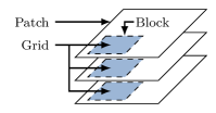
(a)

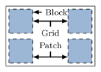
(b)

(c)

(d)

(e)

Figure 3: Examples demonstrating how to map patches to a GPU grid and how to map a spatial block to a thread block. Figure 3a shows several patches that are mapped to one GPU grid and 3b shows one patched mapped to one GPU grid. In Figure 3c the thread block (dashed) is larger than the spatial block (shaded), in 3d a thread block is smaller than the spatial block and in 3e a thread block has the same size as a spatial block.

On multicore CPUs scalable performance is typically achieved using coarse-grained parallelism. The work per thread must be large enough to amortize the overhead of scheduling the work. The block-parallel algorithm in which the spatial blocks are processed in parallel has a potential bottleneck if the work per thread is low for small block sizes. Using the patch parallel method increases the workload per thread so that this bottleneck is avoided. Furthermore, two-level parallelism can improve the performance on a CPU beyond ordinary single-level parallelization [29] especially in comparison to block-level parallelism, which is also demonstrated in Section 4.

2.1 Implementation for CUDA

The implementation of block-relaxation algorithms on GPUs is done using the NVIDIA Compute Unified Device Architecture (CUDA). A short introduction into the technology and programming of CUDA can be found in [30, 31]. Threads in CUDA are grouped together into thread blocks and are executed in a Single Instruction Multiple Threads (SIMT) fashion of 32 threads called a warp. Thread blocks are organized into grids and each CUDA kernel launches one grid of several thread blocks.

The decomposition of a patch in spatial blocks shares similarities with the CUDA architecture. But mapping a spatial block to a thread block or a patch to a grid on the GPU is nontrivial in the case of block smoothing. The mapping has an impact on the level of parallelism that can be achieved using different spatial block and patch sizes. We suggest the following two strategies for processing patches on the GPU:

Strategy 1: One thread block processes all spatial blocks within a patch as in Figure 3a. The thread block sweeps through the patch. In this case a GPU grid maps different thread blocks to different patches. Spatial blocks in different patches are processed in parallel resulting in two-level parallelism.

Strategy 2: One patch is processed by several thread blocks on the GPU as shown in Figure 3b. Here single-level parallelism exists if the patch size is large enough that the maximum number of scheduled thread blocks on the GPU is reached. In this case only one patch can be processed at a time on the GPU. If the patch size is small enough that multiple patches can be processed in parallel, then two-level parallelism is possible.

In this paper we explore Strategy 2 for the presented implementations of the block smoothing relaxation. Strategy 1 will be explored in future research projects. In addition to the patch mapping, the spatial blocks must be mapped to the thread blocks on the GPU. A common method for spatial blocking is overlapping axis-aligned 3D blocking [32], in which a spatial block of dimension $b_{x}\times b_{y}\times b_{z}$ with neighbor cells $\mathcal{R}$ is loaded into on-chip memory, leading to some redundant memory transfers for the neighbor cells. 3D blocking can be optimized by a 2.5D sliced blocking technique such as [33] or [32]. In 2.5D slicing, a block is decomposed into slices of cells. These slices are processed sequentially in an alternative blocking that preserves some cells in the on-chip cache or even registers, reducing global memory access. 2.5D blocking is outside the scope of this paper but will be explored in future work. We focus on 3D blocking of the domain. Methods of creating a mapping from the spatial block to the thread block are:

• Thread blocks are larger than spatial blocks. Several spatial blocks can be processed by one thread block (Figure 3c).

• Thread blocks are smaller than spatial blocks. The thread blocks have to sweep through each spatial block (Figure 3d).

• Thread blocks are the same size as spatial blocks. One thread block processes one block in the spatial domain (Figure 3e).

The 2.5D slicing is the (B) block mapping, where the thread block sweeps through slices of a spatial block. Mapping (C) is used for the implementation of the block smoothing algorithm described in this paper. This mapping differs in two major ways from the other mappings. First, it is not necessary to sweep through the spatial domain, avoiding the introduction of additional for-loops as would be necessary for mapping (B). Second, there is no need for a more fine-grained partitioning like in mapping (A). A fine-grained partition means that in order to identify a corresponding spatial block for a thread in mapping (A) additional indexing must be performed.

In mapping (C) each thread in a thread block $b$ is assigned a 3D index $\left(i,j,k\right)$ corresponding directly to the cell with the cell-centered spatial index. A thread resides in two index spaces: the global 3D space that is the index in the patch and the local 3D space that is the index within a thread block. The global 3D index calculation in CUDA without ghost cells using standard lexicographical ordering can be performed in the following manner:

$$\begin{split}i=blockIdx.x\times blockDim.x+threadIdx.x\\ j=blockIdx.y\times blockDim.y+threadIdx.y\\ k=blockIdx.z\times blockDim.z+threadIdx.z.\end{split}$$ (16)

For the calculations with respect to the ghost cells, the thread index must be shifted by the ghost cell width. The local 3D index is given by the three threadIdx values in CUDA.

Cells of a patch including the ghost values are stored in a 1D array. The right-hand side of Equation (3) needs no ghost values. Accessing both vectors on the GPU kernel requires different indexing. Thus a thread resides in additional 1D index spaces: the global 1D space with and without ghost values. If the on-chip shared memory is used within a thread block, an additional local 1D space is also required. The index calculation for the 1D space is a simple axis projection either on the local $blockDim$ or the global $blockDim\times gridDim$ axis. In the resulting block Jacobi iteration on the GPU, as shown in Algorithm 2, each thread in a thread block $b$ computes the new value of a cell in the physical domain.

Algorithm 2 Block Jacobi algorithm on GPUs.

  {Step 1 - Thread block computes residual}

  $r_{b}=f_{b}-A_{b}u_{b}$

  {Barrier for shared memory update}

  __syncthreads()

  {Step 2 - Thread block computes dgemv}

  $r_{b}=\hat{A}_{b}r_{b}$

  {Step 3 - Thread block advances solution}

  $v_{b}=u_{b}+\omega r_{b}$

  {Step 4 - Swap the vectors}

  $u=v$

In the first step of Algorithm 2 the computation of the block residual $r_{b}$ is performed, including the 7-point stencil operation from Equation (1.1) that each thread performs. The computed residual $r_{b}$ for a particular spatial block $b$ is stored in shared memory on the GPU because all threads in a block must access the residual in order to compute the matrix-vector operation in step 2.

The second step of Algorithm 2 consists of multiplying the block-diagonal inverse $\hat{A}_{b}\in\mathbb{R}^{n\times n}$ (where $n$ is the product of the block dimensions) with the block residual $r_{b}$. Each thread in a thread block performs a dot product for its particular cell. The matrix is stored in column-major ordering to optimize the memory access pattern. Step 3 advances the solution of a spatial block. In the case of Jacobi iteration the relaxation parameter $\omega=0.8$ is used and the new block solution is stored in a second vector $v$. The chaotic block Gauss-Seidel updates the solution to $u_{b}+\omega r_{b}$ with $\omega=1$ without any intermediate vector $v$. Swapping the vector $v$ with $u$ in step 4 is only necessary for the block Jacobi iteration.

A feature of the NVIDIA GPUs is that the GPU supports concurrent data transfers, transfer-execution or kernel-execution overlapping [34]. Depending on the instruction stream in the algorithm, either concurrent data transfers, transfer-execution or kernel-execution overlapping is performed.

For transfer-execution overlapping, the instructions must be executed in depth-first order where for all patches the instruction chain: memory transfer to the GPU, kernel execution and the memory transfer back to the host is executed. In this case the transfers from and to the GPU memory can overlap with kernel execution. To execute kernels concurrently, the sequence of instructions must be in breadth-first order in which the transfer for all patches is started, then the kernel execution for all patches and at last the transfer back to the host for all patches. The overlapping of kernel executions is possible only when the number of blocks executed by one kernel does not exceed the number of blocks that can be scheduled concurrently on the GPU.

2.2 Implementation for a Multicore Architecture

In the serial implementation of block Jacobi, Algorithm 3 will be executed for each patch. The CPU implementation first computes the block residual. After this step the block residual is multiplied with the spatial block inverse in step 2. This is done using the optimized Basic Linear Algebra Subprograms (BLAS) Level-2 (dgemv) function. Step 3 must be executed separately from step 2 because accessing the vector $v$ requires a global 3D index computation. Finally advancing the solution using the block Jacobi update scheme has to be done after all blocks are processed in step 4.

Algorithm 3 is parallelized with OpenMP [35] directives by implementing the single-level and two-level parallelism. OpenMP is a compiler extension that enables portable, automated thread parallelism for multicore CPUs. Additional information about OpenMP programming can be found in [36, 37]. For the single-level parallelism the implementation parallelizes either the processing of patches or the processing of blocks. In the two-level parallelism $p$ threads process the patches and spawn additional $q$ threads to process the blocks.

An OpenMP parallel for loop is used to parallelize in the single-level parallelism over either the blocks or the patches. For the two-level parallelism an OpenMP parallel region is created to parallelize over the patches and an additional region is created to parallelize over the blocks using the OpenMP 3.0 collapse directive to collapse the loops over the 3 dimensions $x,y,z$.

Algorithm 3 Block Jacobi algorithm on CPUs.

  for block index in $Z$ do

     for block index in $Y$ do

        for block index in $X$ do

           {Step 1 - Compute block residual}

           $r_{b}=f_{b}-A_{b}u_{b}$

           {Step 2 - Compute dgemv}

           $r_{b}=\hat{A}_{b}r_{b}$

           {Step 3 - Create block solution}

           $v_{b}=\omega r_{b}$

        end for

     end for

  end for

  {Step 4 - Advance the patch solution}

  $u=u+v$

The chaotic block Gauss-Seidel version of Algorithm 3 uses only the single-level block parallelism or nested parallelism to process the blocks asynchronously.

3 Estimating Spatial Blocking

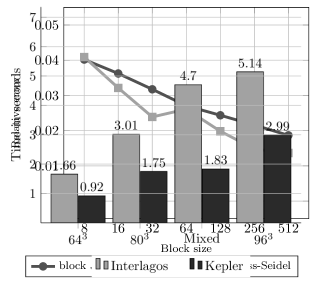
(a) Relative error.

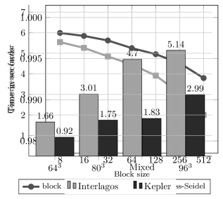
(b) Convergence factor.

Figure 4: Convergence study of block Jacobi and chaotic block Gauss-Seidel relaxation.

The block size in the physical domain influences the convergence and smoothing properties of the algorithm. For multilevel algorithms it is the latter criteria that is of more importance and is also less well understood theoretically other than for specific cases. However, it is important that the algorithm converges all error modes and our numerical experiments in this subsection demonstrate this.

The results of numerical experiments on convergence behavior with different block sizes for block Jacobi and chaotic block Gauss-Seidel relaxations are presented in Figure 4. The following block sizes $\left(b_{x},b_{y},b_{z}\right)$ are used: $\left(2,2,2\right)=8$, $\left(4,2,2\right)=16$, $\left(4,4,2\right)=32$, $\left(4,4,4\right)=64$, $\left(8,4,4\right)=128$, $\left(8,8,4\right)=256$, $\left(8,8,8\right)=512$. We use $\left(4,2,2\right)$ instead of $\left(2,4,2\right)$ or $\left(2,2,4\right)$ because the $x$-dimension provides the fastest memory access in our implementation. We note that for problems with anisotropic coefficients this may not be the best choice.

For the convergence study a patch size of $64^{3}$ is used. The relative error estimate is computed after 3 smoothing steps with a random initial guess. In multigrid applications, performing at most 3 smoothing steps is usually sufficient to smooth the oscillatory error modes. The selection of the $64^{3}$ patch size is based on the volume to surface-area ratio and the overall memory required to store a patch. Considering a ghost cell width of 1, a $32^{3}$ domain with ghost cells needs overall $34^{3}$ cells. The memory overhead to store the ghosts cells is 6536 cells, around 20% of the overall memory needed for $32^{3}$ cells. By using a patch size of $64^{3}$ the overhead is only 10% and for $96^{3}$ only 6%. Larger patches need more memory space so that a patch size of $96^{3}$ requires about 14 Megabytes in double precision to store $u$ and $f$ for all cells in the Gauss-Seidel algorithm and about 21 Megabytes in the Jacobi algorithm. With bigger patches the number of patches that can be processed within a GPU or CPU drops which impacts the balance of the patch distribution across different processes. Choosing patches between $64^{3}$ and $96^{3}$ is a trade-off between the number of patches, memory usage and load balancing.

In Figure 4a the relative error $\left\|{r_{k}}\right\|/\left\|{r_{0}}\right\|$ is shown for different block sizes for $k=3$. Figure 4b shows the asymptotic behavior of the convergence factor $\sqrt[k]{\left\|{r_{i+k}}\right\|/\left\|{r_{i}}\right\|}$ where $i,k$ defines a sliding window for a random initial guess and a large number of smoothing steps ($i\approx 5000$). The asymptotic convergence rate for block Jacobi is reached after a relatively few number of steps while in the case of chaotic block Gauss-Seidel the rate will jitter from step to step because of the chaotic updates but nevertheless the estimation is fairly accurate.

The block Jacobi and chaotic block Gauss-Seidel convergence study shows an overall monotonic improvement in relative error and convergence factor by increasing the block size for a random initial guess. The convergence in smoothing is necessary but does not reflect in general which types of modes have been smoothed and is outside the scope of this paper. However, the convergence behavior serves as a baseline for the performance evaluation with respect to the block size for the presented implementation.

4 Experimental Results

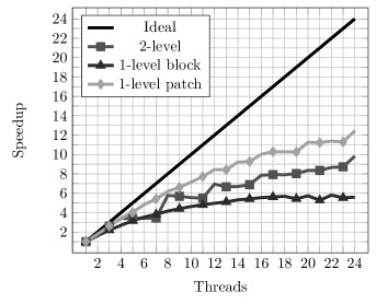
(a) Block Jacobi block size of $4^{3}$.

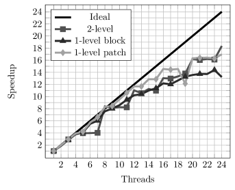
(b) Block Jacobi block size of $8^{3}$.

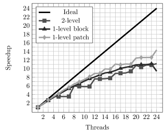
(c) Chaotic block Gauss-Seidel block size of $4^{3}$.

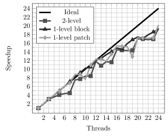
(d) Chaotic block Gauss-Seidel block size of $8^{3}$.

Figure 5: Speedup of block Jacobi and chaotic block Gauss-Seidel relaxation using different levels of parallelism.

This section presents the experimental results for various GPU and multicore CPU implementations of our block smoothing algorithm. In Section 4.1 the speedup of a 24-core Maranello system will be presented. The speedup $S(p)$ of $p$ processors is defined as the fraction of sequential over parallel wall time on $p$ processors. Estimating $S(p)$ with a constant problem size and increasing processor count is called strong scaling. A speedup of $S(p)=p$ is ideal, as the wall time improves proportional to the number of processors that are added. Strong scaling gives a good understanding of how well the algorithm scales with the tested parameter set. We can derive the efficiency $E(p)$ of a parallel system with $p$ processors from the speedup. The efficiency is defined by the ratio $S(p)/p$ between the speedup and the number of processors that reaches the particular speedup.

Section 4.2 compares the wall time of different parameter sets executing the block-relaxation algorithms on the GPUs and CPUs. For the benchmarks different hardwares including a CRAY XK7 node from the “Titan” supercomputer at Oak Ridge National Laboratory are used. Finally in Section 4.3, we provide detailed benchmarks for inverting the diagonal-block matrices of equation (15) with different block sizes. All measurements presented in this section include the update of the ghost cells between patches.

4.1 Multicore Speedup

A state-of-the-art Symmetric Multiprocessing (SMP) compute node equipped with two AMD Opteron 6168 Magny Cours CPUs is used to benchmark the multicore implementations. Each CPU contains 2 dies with 12 cores, and each die has 6 shared 256 bit floating-point units. Using the two-level parallelism 4 threads (number of dies that the system has) are spawned to process the patches in parallel and overall 24 threads are processing the blocks in parallel. Figure 5 shows the strong-scaled speedup for the block Jacobi and chaotic block Gauss-Seidel algorithm processing 96 patches with patch size of $64^{3}$ using two different block sizes. The selected block sizes are $4^{3}$ and $8^{3}$ because the experiments in Section 3 suggest a good convergence factor for $8^{3}$. The block size of $4^{3}$ is used to provide a contrast to the $8^{3}$ with respect to the cost of the matrix-vector multiplication, the inversion of the block diagonal matrix and performance on the GPU and CPU.

Name	Processors	Cores	Speed	GFLOPS	Watts
Interlagos (XE6)	2 $\times$ AMD 6272	$4\times 8=32$	2.1 GHz	$\scriptstyle\sim$295	230
Maranello	2 $\times$ AMD 6168	$4\times 6=24$	1.9 GHz	$\scriptstyle\sim$202	230
Fermi	1 $\times$ NVIDIA C2050	$14\times 32=448$	1.2 GHz	$\scriptstyle\sim$515	238
Kepler (XK7)	1 $\times$ NVIDIA K20X	$14\times 192=2688$	0.73 GHz	$\scriptstyle\sim$1310	235

Table 1: Test systems for the performance benchmarks. The column Cores shows the processor core configuration, the columns Speed and GFLOPS the chip clock speed and the theoretical peak performance in double precision of the cores and the column Watts the power consumption in Watts.

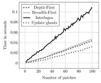
(a) Patch size $16^{3}$ and block size of $8^{3}$.

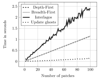
(b) Patch size $64^{3}$ and block size of $8^{3}$.

Figure 6: Chaotic Gauss-Seidel relaxation on Kepler using different overlapping techniques.

The results from the multicore benchmarks show that using the patch-parallelism, block-parallelism or two-level parallelism gives similar scalability, especially when using block size of $8^{3}$ though the patch-parallelism is the best for block size $4^{3}$. A maximum speedup around 18 is reached for the block Jacobi and 20 for chaotic block Gauss-Seidel using block size $8^{3}$.

This leads to an efficiency of about 80% on the 24-core machine. Choosing a block size of $4^{3}$ drops the maximal speedup for both algorithms to about 12 for block Jacobi and 14 for chaotic block Gauss-Seidel. The patch-parallel version of the chaotic block Gauss-Seidel is in fact a standard block Gauss-Seidel relaxation without chaotic updates because the blocks are processed in serial.

A larger block size leads to better scalability with respect to efficiency for both algorithms. The two-level parallelism scales as well as the patch-parallel version and allows the chaotic block update in the Gauss-Seidel scheme.

From the speedup results we see that the block Jacobi algorithm gains more from processing the patches in parallel than processing the blocks in parallel, because the block-parallel version does not scale well with smaller block sizes. The patch-parallel or nested-parallel versions of Jacobi scale better because the solution $u^{k+1}$ is advanced for the patches in parallel. In the case of the chaotic block Gauss-Seidel the block parallel version scales better for smaller block sizes than the two-level parallelism. The stairstep pattern in the speedup of the two-level parallelism indicates a workload imbalance caused by adding block parallelism to the patch parallel version.

4.2 Algorithm Performance

(a) Block Jacobi relaxation.

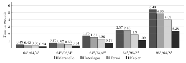
(b) Chaotic block Gauss-Seidel relaxation.

Figure 7: Time to smooth with chaotic block Gauss-Seidel and block Jacobi relaxations. The data is grouped by parameter set (patch size / number of patches / block size) for different systems.

In this section we present measurements that have been taken on the systems listed in Table 1 and from now we reference the system by its name. One system named ‘Maranello’ consists of two AMD Opteron 6168 CPUs and one NVIDIA TESLA C2050 (Fermi) [38]. The other system named ‘Interlagos’ is a CRAY XE6 [39] node equipped with two AMD Opteron 6272 CPUs and a CRAY XK7 node [40] provides the benchmarks for the NVIDIA TESLA K20X (Kepler) GPU [41]. Floating-Point Units (FPUs) on the NVIDIA Fermi GPU are arranged as a set of 32 in each Streaming-Multiprocessor (SM), while on the NVIDIA Kepler GPU, each Streaming-Multiprocessor (SMX) comprises of 192 single-precision CUDA cores, 64 double-precision units, 32 special function units, and 32 load/store units. On the CPUs the arrangements of FPUs are different as for Maranello each die consists of 6 FPUs and for Interlagos each die has 4 FPUs but 8 integer units. The different FPU arrangements reflect one difference between the two AMD architectures. All benchmarks in this section exclude the time to compute the inverses. Timings to compute the inverses are presented in Section 4.3.

The GPU has the option to overlap as described in Section 2.1. A benchmark is used to explore the performance of the different overlapping techniques to estimate which method should achieve the best performance for different patch sizes. Figure 6 shows the wall time for 3 smoothing steps varying numbers of patches and the patch size on the Kepler GPU by exploiting kernel overlapping (breadth-first) or kernel transfer overlapping (depth-first). Figure 6 also shows the wall time for the Interlagos system using the two-level parallelism for comparison.

The depth-first overlapping strategy is slightly better than the breadth-first approach for patch size of $16^{3}$, and they give almost identical timings for patch sizes $64^{3}$. Moreover, they both outperform the CPU timings taken on Interlagos by a factor around 2.5. Note that all these timings include updating the ghost cells among the patches. The bottom line in Figure 6a and 6b is the time required to update the ghost cells. When the patch size is $16^{3}$, updating the ghost cells takes about 70% of the GPU time and 25% of the CPU time, and while the patch size is $64^{3}$, it consumes around 15% of the GPU time and 5% of the CPU time. This indicates that using patch size of $64^{3}$ or larger may be more preferable in AMR applications.

For the benchmarks the focus is on patch sizes of at least $64^{3}$ so that the timings are taken with depth-first asynchronous memory transfer from and to the GPU in each smoothing step, while the CPU implementation does not need to execute memory transfers after each step. Timings for the CPU code are taken from the two-level nested version. In Figure 7 the wall time, smoothing selected parameter sets is shown for the block Jacobi and for chaotic block Gauss-Seidel relaxations.

Three smoothing steps are executed on varying parameter sets. Each parameter set is defined by patch size, number of patches and block size. Sets with patch sizes of $64^{3}$ and $96^{3}$ and block sizes of $4^{3}$ and $8^{3}$ are benchmarked. The Interlagos outperforms the Maranello because of its higher peak performance.

Both GPUs perform better than the multicore systems. The Kepler is faster then the Fermi because of the new architecture and higher peak performance. The wall time using the parameter set ($64^{3}/96/8^{3}$) for both algorithms on the Kepler is about $2.2\times$ faster than the multicore time on the 32-core Interlagos machine.

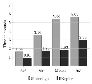
(a) Block Jacobi relaxation.

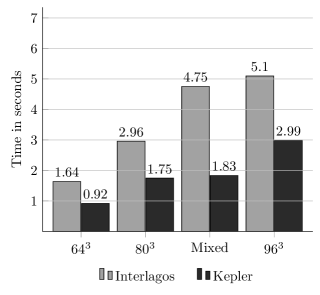
(b) Chaotic block Gauss-Seidel relaxation.

Figure 8: Smoothing sets of patches with the same and with mixed sizes.

Patch size	#	#Cells	Block size
$64\times 64\times 64$	80	62,914,560	$8\times 8\times 8$
$80\times 80\times 80$	80	122,800,000	$8\times 8\times 8$
Mixed	80	130,252,800	$8\times 8\times 8$
$96\times 96\times 96$	80	212,336,640	$8\times 8\times 8$

Table 2: Patch sets for smoothing fixed number of 80 patches using sets of the same and mixed sizes.

The selected application parameter sets use the same patch sizes which are characteristic of one class of AMR methods. However, for another class of AMR applications the patch size can vary. We benchmark the performance of the block smoothers using different patch sizes to better reflect the practical performance for this latter class of AMR methods. For estimating the practical performance, a benchmark executing the smoothing algorithms on patch sets with the same patch sizes and sets with different sizes as listed in Table 2. All sets consist of 80 patches and the mixed patch set is divided into subsets of 16 patches with $64^{3}$, $72^{3}$, $80^{3}$, $88^{3}$ and $96^{3}$. The ratio of cells between $64^{3}$ and $80^{3}$ is 1.89 and the ratio of cells between $64^{3}$ and the mixed set is 2.07. The ratio of cells between $80^{3}$ to $96^{3}$ is 1.72 and the ratio of cells between mixed and $96^{3}$ is 1.63.

Figure 8 shows the wall time for smoothing patches of the same and mixed sizes using block Jacobi or chaotic block Gauss-Seidel on the fastest GPU and the CPU system. The time for smoothing the patches on the GPU increases roughly proportionally to the number of cells independent of the mixed patch sizes for both algorithms. This behavior is expected because no synchronization is needed at the end of a processed patch and the memory transfer overlaps with the kernel execution. Essentially the GPU just batch processes block after block without stalling. However, the behavior is not the same in the CPU implementation. In the CPU implementation the wall time increases proportionally to the patch size for constant-size patches. For the mixed patch size set the wall time is closer to the time that is needed to smooth the largest patches. The reason for the poor performance of the mixed set is that the OpenMP threads looping over the blocks must join after the patches are processed, and end up waiting for the largest patches.

Load balancing in the case of mixed patch sizes is an issue that depends on the ordering of the patches. In reality, the ordering of patches is random and in the worst case one thread gets all the larger patches. Using a naive approach by partitioning the patches without respect to the size has a potential for imbalance. The computation of an optimal partitioning is a variation of the bin packing problem which is known to be NP-hard. We can control the ordering of patches in the benchmark and if the patches are partitioned perfectly (each thread has the same amount of work) then the wall time for the mixed set drops to 4.37 seconds for block Jacobi and 3.96 seconds for chaotic block Gauss-Seidel.

Smoothing using mixed patch sizes accelerates the GPU wall time more than $2.9\times$ over the CPU wall time in the case of block Jacobi relaxation and chaotic block Gauss-Seidel when the patches are imbalanced. A balanced patch partitioning improves the wall time on the CPU for the mixed set, but to be fair the additional cost for partitioning must be taken into consideration because it is not necessary on the GPU.

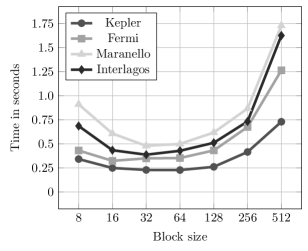
Figure 9: Kernel performance for chaotic block Gauss-Seidel using different block sizes with patch size $64^{3}$.

But as discussed in Section 3, another important factor contributing to the wall time is the block size. The number of floating-point operations for the stencil is constant for a thread in a thread block regardless to the block size, so the performance is dominated by the matrix-vector multiplication of the block inverse with the residual. Figure 9 shows the wall time for smoothing 3 iterations on 64 patches with a patch size of $64^{3}$ using different block sizes for the chaotic block Gauss-Seidel method.

The GPU outperforms the CPU for all cases considered. For a block size of $8^{3}$ more than 67 million cells per second can be smoothed on the Kepler and around 31 million cells per second on the Interlagos.

4.3 Block inversion

Our block-relaxation algorithms require block inversions of diagonal blocks from the matrix that corresponds to the discretization over the AMR domain. In the case of constant-coefficient stencils the computation of the inverse must be performed only once if the patch size is a multiple of the block size. If the patch size is not a multiple of the block size then two possibilities exist. Either the blocks that do not fit at the end of the patch overlap with the previous ones, which can potentially change the convergence behavior, even resulting in divergence of the smoothing algorithm for chaotic updates, or all inverses for these cases must be precomputed.

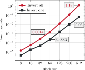
Figure 10: Total time to compute the inverse of either one matrix or all block matrices for different block sizes.

Computing all inverses is a robust approach that needs more memory and more computation time upfront. A total of $b_{n}=b_{x}b_{y}b_{z}$ inverses are potentially needed for a block of size $b_{x}\times b_{y}\times b_{z}$. To estimate the inverse computation overhead a benchmark computes either one inverse for a block or all inverses for a particular block size as shown in Figure 10.

The inversion is performed using a sequential BLAS library on the Interlagos system. Computing the inverses can be done in parallel but the cost of computing the inverses in serial is negligible in both cases. For example, computing the inverse of the block size $8^{3}$ takes 0.06 seconds on Interlagos, or about 4% of the wall time of 1.51 seconds needed for one simulation iteration smoothing three steps with 64 patches of size $64^{3}$ using chaotic block Gauss-Seidel on the same system. In the case of multiple inverses this fraction increases but is also negligible because the inverses have to be computed only once for the whole simulation in the case of constant-coefficient stencils and therefore the time for precomputing the inverses is amortized over a few simulation steps. For example, in our typical AMR simulations the inverses can be reused thousands of times.

5 Conclusions and Future Work

We implemented our block smoothing algorithm for structured adaptively refined meshes using block Jacobi and chaotic block Gauss-Seidel relaxations for modern GPUs and multicore CPUs. Our multicore implementation scales on a 24-core machine with an efficiency of 80%, achieving a speedup around 20 by exploring multiple parallel strategies. The GPU version is about $2.2\times$ faster than our best multicore system using patches of the same sizes. In practical benchmarks with mixed patch sizes we can observe about $2.9\times$ improvement using a GPU. The peak performance of Kepler is about $4.4\times$ the peak of the newest CRAY XE6 compute node. An overall wall time acceleration from $2.2\times$-$2.9\times$ on Kepler is a good result but there is still room to improve both implementations.

The way asynchronous memory transfer on the GPU will be issued does not have an impact on the Kepler GPU. Comparing the block Jacobi with the chaotic block Gauss-Seidel shows that both algorithms scale in the same fashion and the chaotic block Gauss-Seidel algorithm gives a better wall time. The chaotic block Gauss-Seidel gives better results in terms of convergence and relative error for the random initial guess for almost all tested block sizes. Increasing the block size further improves the convergence factor for both algorithms.

In addition we presented strategies for the parallelization of the block smoothing algorithm in the context of adaptively refined meshes. Different abstract mapping strategies for the GPU were also presented and can be used independently from the smoothing in future structured AMR-based algorithms. The implemented OpenMP versions use single-level and two-level parallelism approaches to realize these mappings.

Our future investigation is to optimize our block-relaxation implementations for the next hybrid supercomputer architecture by exploring more GPU parallelism like tiling the blocks or other patch mapping strategies. Moreover a hybrid implementation by smoothing patches on the GPU and CPU is necessary because the memory transfer and kernel execution on the GPU is asynchronous so that the CPU is idle during the processing on the GPU. This wasted compute power can be used in future implementations. We also plan to use the implemented block relaxation algorithms in multilevel preconditioners to solve complicated multi-physics problems on distributed systems.

References

- [1]
- [2] U. Trottenberg, C. Oosterlee, and A. Schüller. Multigrid. Academic Press, 2001.
- [3] W. Briggs, V. Henson, and S. McCormick. A Multigrid Tutorial 2nd Edition. Philadelphia: SIAM, 2000.
- [4] Y. Saad. Iterative Methods for Sparse Linear Systems, 2nd ed. Philadelphia, PA, USA: SIAM, 2003.
- [5] M. Kowarschik, I. Christadler, and U. Rüde. “Towards cache-optimized multigrid using patch-adaptive relaxation,” in PARA, 901–910, 2004.
- [6] S. Schaffer. A semicoarsening multigrid method for elliptic partial differential equations with highly discontinuous and anisotropic coefficients. SIAM Journal on Scientific Computing, 20(1): 228–242, Dec. 1998.
- [7] J. Dendy. Black box multigrid. Journal of Computational Physics, 48(3): 366 – 386, 1982.
- [8] S. F. McCormick and J. W. Thomas. The Fast Adaptive Composite grid (FAC) method for elliptic equations. Math. Comp., 46: 439–456, 1986.
- [9] A. Brandt. Multi-Level Adaptive Solutions to Boundary-Value Problems. Mathematics of Computation, 31(138): 333–390, Apr. 1977.
- [10] G. H. Shortley and R. Weller. The Numerical Solution of Laplace’s Equation. Journal of Applied Physics, 9(5): 334–348, 1938.
- [11] S. V. Parter. Multiline iterative methods for elliptic difference equations and fundamental frequencies. Numerische Mathematik, 3(1): 305–319, 1961.
- [12] B. Philip and T. P. Chartier. Adaptive algebraic smoothers. Journal of Computational and Applied Mathematics, 236(9): 2277–2297, Mar. 2012.
- [13] Z. Feng and P. Li. Multigrid on GPU: tackling power grid analysis on parallel SIMT platforms. In Proceedings of the 2008 IEEE/ACM International Conference on Computer-Aided Design, ser. ICCAD ’08. Piscataway, NJ, USA: IEEE Press, 647–654, 2008.
- [14] H. Anzt, S. Tomov, M. Gates, J. Dongarra, and V. Heuveline. Block-asynchronous multigrid smoothers for GPU-accelerated systems. Innovative Computing Laboratory, University of Tennessee, UT-CS-11-689, Tech. Rep., 2011.
- [15] S. Venkatasubramanian and R. W. Vuduc. Tuned and wildly asynchronous stencil kernels for hybrid CPU/GPU systems. In Proceedings of the 23rd International Conference on Supercomputing, ser. ICS ’09. New York, NY, USA: ACM, 244–255, 2009.
- [16] M. Adams, M. Brezina, J. Hu, and R. Tuminaro. Parallel multigrid smoothing: polynomial versus Gauss-–Seidel. Journal of Computational Physics, 188(2): 593–610, 2003.
- [17] M. F. Adams. A distributed memory unstructured Gauss–Seidel algorithm for multigrid smoothers. In Proceedings of the 2001 ACM/IEEE conference on Supercomputing (CDROM), ser. Supercomputing ’01. New York, NY, USA: ACM, 4–4, 2001.
- [18] R. Guy, B. Philip, and B. Griffith. A multigrid method for the coupled implicit immersed boundary equations. Invited talk, May 2012, the Second International Conference on Scientific Computing (ICSC12), Nanjing, China.
- [19] B. Philip, L. Chacón, and M. Pernice. Implicit Adaptive Mesh Refinement for 2D reduced resistive magnetohydrodynamics. Journal of Computational Physics, 227(20): 8855–8874, Oct. 2008.
- [20] M. Pernice and B. Philip. Solution of equilibrium radiation diffusion problems using implicit Adaptive Mesh Refinement. SIAM Journal of Scientific Computing, 27(5): 1709–1726, Nov. 2005.
- [21] R. S. Varga. Matrix Iterative Analysis. San Diego, CA: Springer Series in Computational Mathematics, 1999.
- [22] D. Chazan and W. Miranker. Chaotic relaxation. Linear Algebra and its Applications, 2(2): 199–222, 1969.
- [23] A. Frommer and D. B. Szyld. On asynchronous iterations. Journal of Computational and Applied Mathematics, 123(1-2): 201–216, Nov. 2000.
- [24] G. M. Baudet. Asynchronous iterative methods for multiprocessors. Journal of the ACM, 25(2): 226–244, Apr. 1978.
- [25] J. C. Strikwerda. A probabilistic analysis of asynchronous iteration. Linear Algebra and its Applications, 349(1–3): 125–154, 2002.
- [26] D. Bertsekas and J. Tsitsiklis. Parallel and distributed computation: numerical methods. Prentice Hall, 1989.
- [27] J. C. Strikwerda. A convergence theorem for chaotic asynchronous relaxation. Linear Algebra and its Applications, 253(1–3): 15–24, 1997.
- [28] K. Blathras, D. B. Szyld, and Y. Shi. Timing models and local stopping criteria for asynchronous iterative algorithms. Journal of Parallel and Distributed Computing, 58: 446–465, 1999.
- [29] R. Blikberg and T. Sørevik. Load balancing and OpenMP implementation of nested parallelism. Journal of Parallel Compututing, 31(10-12): 984–998, Oct. 2005.
- [30] J. Nickolls, I. Buck, M. Garland, and K. Skadron.Scalable parallel programming with CUDA. Queue, 6, March 2008.
- [31] D. B. Kirk and W. W. Hwu. Programming Massively Parallel Processors: A Hands-on Approach. 1st ed. Morgan Kaufmann, 2010.
- [32] A. Nguyen, N. Satish, J. Chhugani, C. Kim, and P. Dubey. 3.5-D Blocking optimization for stencil computations on modern CPUs and GPUs. In Proceedings of the 2010 ACM/IEEE International Conference for High Performance Computing, Networking, Storage and Analysis, ser. SC ’10. Washington, DC, USA: IEEE Computer Society, 1–13. 2010.
- [33] P. Micikevicius. 3D finite difference computation on GPUs using CUDA. In Proceedings of 2nd Workshop on General Purpose Processing on Graphics Processing Units, ser. GPGPU-2. New York, NY, USA: ACM, 79–84, 2009.
- [34] NVIDIA Corporation. NVIDIA CUDA C Programming Guide. 2012.
- [35] OpenMP Application Program Interface. http://www.openmp.org/mp-documents/spec30.pdf. 2008.
- [36] R. Chandra, R. Menon, L. Dagum, D. Kohr, D. Maydan, and J. McDonald. Parallel Programming in OpenMP. Morgan Kaufmann Publishing, 2000.
- [37] B. Chapman, G. Jost, R. van der Pas, and D. J. Kuck. Using OpenMP: Portable Shared Memory Parallel Programming. The MIT Press, 2007.
- [38] NVIDIA Corporation. The NVIDIA TESLA C2050 and C2070 computing processors. http://www.nvidia.com/docs/IO/43395/NV_DS_Tesla_C2050_C2070_jul10_lores.pdf. 2010.
- [39] CRAY Inc.. CRAY XE6 online product brochure. http://www.cray.com/Assets/PDF/products/xe/CrayXE6Brochure.pdf. 2011.
- [40] CRAY Inc.. CRAY XK7 online product brochure. http://www.cray.com/Assets/PDF/products/xk/CrayXK7Brochure.pdf. 2012.
- [41] NVIDIA Corporation. NVIDIAs Next Generation CUDA Compute Architecture: Kepler TM GK110. http://www.nvidia.com/content/PDF/kepler/NVIDIA-Kepler-GK110-Architecture-Whitepaper.pdf. 2012.