Electron-like Fermi surface and in-plane anisotropy due to chain states in YBa₂Cu₃O_7-δ superconductors

Abstract

We present magneto-transport calculations for YBa₂Cu₃O_7-δ (YBCO) materials to show that the electron-like metallic chain state gives both the negative Hall effect and in-plane anisotropic large Nernst signal. We show that the inevitable presence of the metallic 1D CuO chain layer lying between the CuO₂ bilayers in YBCO renders an electron-like Fermi surface in the doping range as wide as $p=0.05$ to overdoping. With underdoping, a pseudogap opening in the CuO₂ state reduces its hole-carrier contribution, and therefore the net electron-like quasiparticles dominate the transport properties, and a negative Hall resistance commences. We also show that the observation of in-plane anisotropy in the Nernst signal – which was taken as a definite evidence of the electronic ‘nematic’ pseudogap phase – is naturally explained by including the ‘quasi-uniaxial’ metallic chain state. Finally, we comment on how the chain state can also lead to electron-like quantum oscillations.

An understanding of the pairing mechanism in cuprate superconductors relies on the underlying complex Fermi surface (FS) properties, and how they are derived from the normal state pseudogap (PG) phase. Important clues to the origin of the PG state have been put forward by recent Hall effect measurements which observed a negative Hall resistance below the PG temperature in YBCO systems.HallEP This result received further supports from the negative Seebeck coefficient,seebeck ; seebeckNC strongly enhanced Nernst effect,Nernst_nematic ; Nernst_data as well as identification of quantum oscillationsSdH2007 ; SdH2008 ; sebastian_compensated ; sebastianmass ; QOPDai with cyclotron frequency indicative of electron-like FS. These stimulating discoveries, which according to the conventional Onsager-Lifshitz paradigmOnsagar implies a closed electron pocket, point toward the topological changes in the FS in the PG state when compared with its large metallic FS in the overdoped sample.ARPES_damascelli Such small electron pockets do not arise naturally from the band-structure calculations considering the CuO₂ planes and their total area is inconsistent with the nominal doping concentration.LDA

To explain these results, candidate proposals for various symmetry-breaking patterns have been offered, leading to drastic FS reconstruction into multiple Fermi pockets of different natures.Norman ; Norman_Lifshitz ; DDW ; DasSDW ; fldCO ; Harrison ; Sachdev_SDW ; DDW_Nernst We would, however, expect to see signatures of these pockets in spectroscopies such as angle-resolved photoemission spectroscopy (ARPES) and scanning tunneling microscopy/spectroscopy (STM/S). Yet, extensive ARPESARPES_damascelli ; ARPES_borisenko , and STMSTM_FA studies on various cuprate materials consistently have so far been able to map out only one Fermi pocket or ‘Fermi arc’ – both would represent the same FS segment if the intensity on the pocket’s back side is suppressed by the coherence factors – which is again of hole-like character.DDW ; DasSDW Furthermore, to explain the large negative Hall coefficient, one requires to have electron-like quasiparticles dominating over the hole quasiparticles on the FS, which is prohibited in hole doped system due to Luttinger theorem. On the basis of this reasoning, the recent experimental evidence of a field induced charge orderingfldCO will also find difficulty in explaining the negative Hall coefficient even if it is assumed to induce electron pocket.Harrison Taken together, the electron-pocket scenarios of various density wave originsNorman ; DDW ; DasSDW ; Harrison are inadequate to explain the negative slope of the magneto-transport data.

In this study, we introduce a fundamentally new perspective – we show that the emergence of the electron-like FS in the PG state can be rationalized by realistically considering the contributions of the much ignored metallic CuO chain bands in YBCO. The unambiguous existence of the chain states on the FS has been well established by many ARPES studies from extreme underdoped region ($p=0.05$) to overdoping ($p=0.29$ and above).ARPES_damascelli ; ARPES_borisenko Its contribution to $c$-axis transportHussey and quantum oscillation in specific heatRiggs measurements is also studied earlier, further supporting the metallic character of chain state. The chain states seem to exhibit neither the PG opening nor any considerable doping dependence. Nevertheless, it dominates in the electronic spectra in the PG state due to its interplay with the CuO₂ states. Our reasoning that underlies this conclusion is that the PG opens in the CuO₂ bilayers, truncating its full metallic FS into small segments. Irrespective of the specific origin and nature of the small FS, it contains much reduced hole-carrier concentrations, determining the nominal hole doping of the sample. Therefore, the low-energy electronic state becomes effectively characterized by electron-like charge carriers of the chain state. Above the PG regime both in temperature ($T$) and doping ($p$), the large CuO₂ state is recovered, restoring the predominant hole-carrier on the FS of YBCO. The resulting two-carriers FSs quantify the negative Hall effect,HallEP and also the enhanced Nernst signal with prominent in-plane anisotropyNernst_nematic ; Nernst_data due to the ‘quasi-uniaxial’ character of the chain state.

Tri-layer lattice model:- Encouraged by the ARPES resultsARPES_damascelli ; ARPES_borisenko and the first-principle calculations,LDA we formulate a unified non-interacting three band model, originating from 2D CuO₂ bilayers and an 1D CuO chain.atkinson ; footortho To effectively model the reminiscent nodal FS segment of the CuO₂ bands in the PG state, we consider some form of density-wave order whose front side would also accommodate the ‘Fermi arc’ property. Constrained by this assumption, a Hartree-Fock like order parameter is introduced to the Hamiltonian with a periodic modulation ${\bm{Q}}=(\pi,\pi)$, which is commensurate with the CuO₂ lattice plane. We can think of a residual spin-DasSDW or charge-density wavefldCO (S/CDW) or a $d$-density waveDDW or some other commensurate FS instability as the microscopic origin of such ordering, however, the macroscopic properties we aim to describe here do not rely on these details.DasSDW On the basis of these experimental considerations, we deduce the general form of the Hamiltonian in the Nambu representation per unit cell:

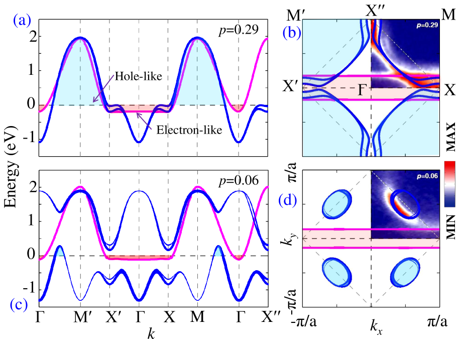
Figure 1: (Color online) (a) Paramagnetic dispersion obtained from the eigenstates of the Hamiltonian in Eq. 1. Blue lines are the bonding and antibonding bands arising from the CuO₂ planes, while magenta line depicts the chain state. The light blue and red shadings represent the hole-like and electron-like character of the bands, respectively. (b) Corresponding computed FSs are compared with the ARPES dataARPES_damascelli (plotted only in one quadrant of the Brillouin zone for visualization). (c) Same as in (a), but computed in the PG state in an underdoped region. The width of each line gives the associated spectral-weight, determined by the SDW coherence factors. (d) FSs in the PG state host only tiny hole pockets centering nodal points.

$$H=\sum_{{\bm{k}}\sigma,ij}\left[\xi_{ij{\bm{k}}}c_{i{\bm{k}}\sigma}^{{\dagger}}c_{j{\bm{k}}\sigma}+V_{ij{\bm{k}}}c_{i({\bm{k}}+{\bm{Q}})\sigma}^{{\dagger}}c_{j{\bm{k}}\bar{\sigma}}+h.c.\right],$$ (1)

where $c_{i{\bm{k}}\sigma}^{{\dagger}}~{}(c_{i{\bm{k}}\sigma})$ creates (annihilates) an electron with momentum ${\bm{k}}$ and spin $\sigma$ on the $i=p,p^{\prime},c$ tri-layers. The singe-particle dispersions $\xi_{ij}$ are defined within tight-binding expansion of the Cu $d_{x^{2}-y^{2}}$-orbitals (hybridized intrinsically with O $p$ orbitals) hopping on a periodic lattice in the tetragonal crystal as given in Ref footTB, .

Next, we exemplify how a small hole-pocket forms in the PG state. To simplify the analysis, while retaining the salient spectroscopic features, we adopt a ${\bm{k}}$-independent interaction potential $V$ to be same for both bilayers states, while setting $V=0$ for the chain layer, as the latter do not exhibit any PG opening. We set the spin index $\bar{\sigma}=-\sigma$ to construct a SDW modulation. In this case, $V$ encodes the onsite Hubbard $U$, and a order parameter $S$, as $V_{i}=US_{i}$, with $S_{i}=\langle c^{{\dagger}}_{i({\bm{k}}+{\bm{Q}})\sigma}c_{i{\bm{k}}\sigma}\rangle$ ($i=p,p^{\prime}$), where the canonical average is taken over the entire Brillouin zone. We use the value of effective $U$=1.59 eV, deduced from earlier calculations,DasSDW ; Dahm and the order parameter $S$ is evaluated self-consistent at each $T$ and doping. See supplementary materialSM for details. We emphasize that our choice of a particular form of density wave does not preclude us from analyzing the full problem, rather improves the reliability of the results with respect to a single parameter $U$. The choice of ${\bm{Q}}=(\pi,\pi)$ order however gives the FS topology which agrees well with most ARPES data.

In Figs. 1(c) and (d), we notice that a direct band gap is opened at $E_{F}$ everywhere in the Brillouin zone, except at the nodal points, giving rise to a hole-pocket in the CuO₂ states. The width of each line depicts the associated quasiparticle weight which is in detailed agreement with experiments, given that the weak intensity of the shadow bands can be detected by ARPES.JMesot ; ZXshadow It is important to note that while the parameters of the chain states are doping independent, its electronic states posses a weak doping evolution via the interlayer coupling to the plane states. It is self-evident from the band curvature of the chain states at $E_{F}$ that it continues to host electron-like FS (although open orbit) at all doping; see Fig. 2 for further illustration. The electron-like property of the chain state is also evident in the ARPES data of Ref. ARPES_damascelli, .

Hall and Nernst effect calculation:- Relying on the aforementioned effective normal state Hamiltonian for YBCO, we now proceed to study the quasi-particle transport properties based on a semiclassical numerical calculation. Nernst experiment measures the transverse electric field, ${\bm{E}}$, in response to a combination set-up of an externally-imposed temperature gradient, $\nabla T$, and an orthogonal magnetic field, ${\bm{B}}$.Nernst_nematic ; Nernst_data The net electric current density ${\bm{J}}$ produced via this effect is essentially related to ${\bm{E}}$ and $\nabla T$ via linear response in-plane Hall conductivity tensor $\hat{\sigma}$ and Nernst conductivity tensor $\hat{\alpha}$, as ${\bm{J}}$=$\hat{\sigma}{\bm{E}}$-$\hat{\alpha}\nabla T$. In case of a perfect cancelation of the net charge current, we obtain a working formula for these two measured quantities: ${\bm{E}}=\hat{\sigma}^{-1}\hat{\alpha}\nabla T=-\hat{\theta}\nabla T.$ Experimentally, the Hall resistance, $\hat{\rho}$=$\hat{\sigma}^{-1}$, and the Nernst coefficient, ${\nu}$=$\hat{\theta}/B$, are measured independently via transport probes typically by setting a weak magnetic field ${\bm{B}}$=$B\hat{z}$ along the $c$-axis of the lattice.HallEP ; Nernst_nematic

In theory, $\hat{\sigma}$ and $\hat{\alpha}$ are calculated by solving the standard Boltzmann equations for the low-$T$ DC transport.Sachdev_SDW ; DDW_Nernst After some tedious algebra we derive the formalism for these quantities in terms of the quasiparticle states and their associated weight (see supplementary materialSM ):

$$\hat{\sigma}_{\mu\nu}^{ij}=\frac{\beta e^{2}}{2}\sum_{{\bm{k}},n}M_{n{\bm{k}}}^{ij}v^{\mu}_{n{\bm{k}}}\Omega_{n{\bm{k}}}^{-1}v^{\nu}_{n{\bm{k}}}{\rm sech}^{2}\left(\frac{\beta E_{n{\bm{k}}}}{2}\right),\hskip 22.0pt$$ (2)

$$\hat{\alpha}_{\mu\nu}^{ij}=-\frac{\beta^{2}e}{2}\sum_{{\bm{k}},n}M_{n{\bm{k}}}^{ij}v^{\mu}_{n{\bm{k}}}\Omega_{n{\bm{k}}}^{-1}v^{\nu}_{n{\bm{k}}}E_{n{\bm{k}}}{\rm sech}^{2}\left(\frac{\beta E_{n{\bm{k}}}}{2}\right).$$ (3)

Here $E_{n{\bm{k}}}$ stands for the quasiparticle band with wavevector ${\bm{k}}$, and band index $n$, of Hamiltonian in Eq. 1. Denoting the corresponding Bloch eigenstate by $\psi^{i}_{n{\bm{k}}}$, we express the transport matrix-element $M_{n{\bm{k}}}^{ij}=\psi^{i}_{n{\bm{k}}}\psi^{j{\dagger}}_{n{\bm{k}}}$. $M$ essentially projects the transport tensors from the Bloch quasiparticle representation to the tri-layer lattice indices $i,j$. $v^{\mu}_{n{\bm{k}}}=\partial E_{n{\bm{k}}}/\hbar\partial{\bm{k}}_{\mu}$ is the quasiparticle velocity along the $\mu=x,y,z$ axes, and $\beta=1/k_{B}T$, where $k_{B}$ is Boltzmann constant. The differential operator that drives the system into a non-equilibrium state in response to the applied field is evaluated within relaxation-time approximationRelaxA : $\Omega_{n{\bm{k}}}=\left[-\frac{e}{\hbar c}({\bm{v}}_{n{\bm{k}}}\times{\bm{B}})\cdot\nabla_{\bm{k}}+\tau^{-1}_{\bm{k}}\right]$, where the relaxation time is taken to be constant both in ${\bm{k}}$ and $T$.foottau $e$, $\hbar$ and $c$ have their usual meanings.

The accurate evaluation of the $T$-dependence of the transport properties requires an experimentally constrained $T$-dependent gap parameters, in other words, an accurate description of the $T$-evolution of the FS topology. It is well known that a mean-field order parameter overestimates the PG transition temperature.DasSDW ; Sachdev_SDW To overcome this difficulty, we adopt a phenomenological form of the $T$-dependence of the gap parameter $V(T)$=$V\sqrt{1-T/T_{s}}$,Sachdev_SDW ; TdepPG with the onset $T$ for the density wave order is set to be $T_{s}\approx 55$ K, in close agreement with Neutron measurement for Nd-doped La-based cuprateTs . However, at each $T$, the Fermi level is evaluated self-consistently to preserve the hole counting.

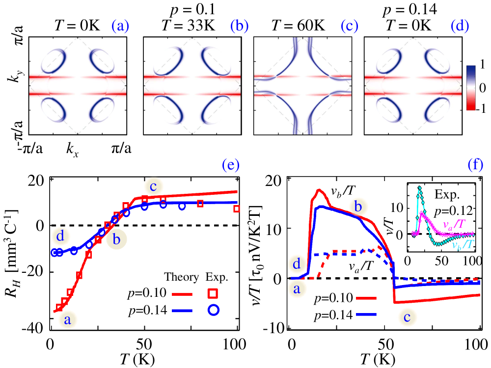
Figure 2: (Color online) (a)-(d) 2D color plots of the total ‘quasi-charge-weight’ $\mathcal{C}_{ij}({\bm{k}},E_{F})$ (averaged over all layers) plotted at four representative cases. The red-white-blue color scheme gives the electron-like quasiparticle to no quasiparticle to hole-like quasiparticle states at a given ${\bm{k}}$ on the FS. (a) ‘Quasi-charge-weight’ calculated at an extreme low-$T$ region for doping $p=0.10$, where the Hall coefficient, $R_{H}$ is negative and Nernst coefficient, $\nu/T$, is small, demonstrating the dominance of the electron-like quasiparticle state on the FS. (b) is chosen at an intermediate $T$ where ‘quasi-electron’ and ‘quasi-hole’ weight compensate each other to lead to zero Hall coefficient and enhanced Nernst signal. At a higher $T$ in (c) SDW disappears and the ‘quasi-hole’ weight dominates. Here Hall and Nernst coefficients flip sign. The plot in (d) is similar to that in (a), but at a higher doping $p=0.14$. It should be noted here that, unlike in a strict ambipolar state, the maximum of the Nernst signal shifts from the zero of Hall coefficient, due to overlapping FS topology and matrix-element effects. (e) The computed $T-$evolution of the Hall coefficient, $R_{H}$, is compared with corresponding experimental dataHallEP at two representative dopings of YBCO. The excellent agreement below the SDW temperature can be clearly marked. (f) Corresponding computed $T$-evolution of the Nernst coefficient, $\nu_{a}=\nu_{xy}$ and $\nu_{b}=\nu_{yx}$, at same $T$ as in (e). The experimental data for YBCO (shown in inset) is available at a slightly different doping.Nernst_data Despite a characteristically good agreement between theory and experiments, we expect discrepancies due to the relaxation time approximation as mentioned in the text. Results of $\nu_{a}$ and $\nu_{b}$ reveal a large anisotropy, which is $T$-dependent. The source is this anisotropy is the presence of the ‘quasi-uniaxial’ chain state, lying along the $y$-axis of the crystal. The anisotropy is strongest when the Nernst signal attains its maximum, in good agreement with experimental data taken from Ref. Nernst_data

Results:- Fig. 2 displays the $T-$evolution of the Hall coefficient $R_{H}=\rho_{yx}/B$ and Nernst coefficient $\nu_{yx}/T$ at two dopings at which the normal state Hall coefficient data are available (the value of $B$ is scaled out in the presented results). A visual comparison between theory and experiment reveals a systematic agreement between them. To relate the sign and magnitude of $R_{H}$ and $\nu_{yx}/T$ to their corresponding charge carrier features, we introduce a function called ‘quasi-charge weight’, in analogy with the quasi-particle weight: $\mathcal{C}_{ij}({\bm{k}},\omega=E_{F})=\sum_{n,{\bm{k}}}e_{n{\bm{k}}}\psi^{i}_{n{\bm{k}}}\psi^{j{\dagger}}_{n{\bm{k}}}\delta(\omega-E_{n{\bm{k}}})$, where $e_{n{\bm{k}}}=\pm e$ at electron and hole like $k_{F}$ obtained from the slope of the bands at $E_{F}$, respectively, for $n^{th}$ band. We emphasize that in the orthorhombic real-space unit cell, the Hall current arises due to finite tunneling between two adjacent chain layers (which gives a warped chain FS in the $k$-space). We plot the total the ‘quasi-charge weight’ in Fig. 2a to d for several representative cases where the Hall coefficient is negative, zero and positive as a function of $T$ and doping.

The obtained results confirm our aforementioned postulates that at low-$T$ when the strong PG shrinks the CuO₂ states into small hole-pockets, the dominant chain states produce a net electron-like quasiparticle character on the FS. With increasing $T$ when the strength of the PG reduces, the area of the hole-pocket gradually increases, while the chain state remains very much unperturbed (note that with increasing hole-pocket area, the self-consistency allows the associated coherence factors to adjust themselves to maintain the same doping concentrations). At some intermediate temperature, $T_{m}$, the ‘quasi-hole’ and ‘quasi-electron’ weights exactly cancel each other to make $R_{H}$ vanishes; see Fig. 1(b). At $T>T_{m}$, the larger hole-pocket reverses the sign of the Hall-resistance, in Fig. 1(e). Finally, above the SDW temperature, the metallic state is restored and the Hall coefficient becomes featureless. The same analysis applies to the higher doping result in that doping reduces the PG order, rendering a smaller hole-pocket, and hence less transport contribution. The results are in excellent agreement with the corresponding experimental dataHallEP , plotted with symbols in Fig. 2(e) and (f).

The discussion of Nernst effect proceeds similarly, although the fundamental mechanism for the enhanced Nernst signal is somewhat different. Experimentally, it is well established that the Nernst signal changes sign from negative to positive as well as it becomes abruptly enhanced below the PG temperature, but much above the superconducting transition temperature, $T_{c}$,Nernst_nematic ; Nernst_data see inset to Fig. 2(f). Despite some proposals that there exists vortex-type excitations even above $T_{c}$ which can drive Nernst signalNernst_prepairing , the widely used ambipolar phenomena suggests that the compensating electron-like and hole-like FSs are primarily necessary to obtain an enhanced ‘normal state’ Nernst signal.ambipolar ; Sachdev_SDW ; DDW_Nernst Within the present theory, such ambipolar state naturally evolves in the vicinity of the intermediate temperature $T_{m}$, where ‘quasi-hole’ and ‘quasi-electron weights’ become comparable, and a positive maximal of Nernst signal arises, as shown in Fig. 2(b). Quantum-oscillation measurement has also detected similar compensating electron- and hole-like FSs in YBCO.sebastian_compensated Away from this $T$ region, the positive Nernst signal diminishes as the underlying states depart from predominant ambipolar character, that is, when only one type of ‘quasi-charge weight’ dominates the excitation spectrum. Interestingly, even when the metallic state appears above the onset temperature of the density wave order, the so-called Sondheimer cancelation of the Nernst signal in a metallic state is still not strictly applicable here due to the coexistence of two-carrier charges on different bands.Sondheimer In fact, the finite experimental value of the Nernst signal above $T_{s}$, which remained an unexplained puzzle in the existing theories, is surprisingly well reproduced within the present theory. The results capture the salient experimental features of YBCO data available at a slightly different doping,Nernst_data ; Nernst_data_foot although some discrepancies are clearly visible. The adopted relaxation time approximation imposes limitation to quantitatively map out the detailed shape and peak positions of the Nernst signal. Furthermore, the present linear-response theory is mainly applicable to the low magnetic field region; on the other hand, experimentally it requires sufficiently high field to expose the ‘normal state’ Nernst signal. Despite these approximations, the Hall and Nernst anomalies are robust features in YBCO, tied to the underlying electronic structure that is confirmed by ARPESARPES_damascelli ; ARPES_borisenko and first-principle resultsLDA .

In-plane anisotropy:-The added benefit of the present theory is that the existence of the the quasi-1D chain state naturally explains the associated in-plane anisotropy in the Nernst signal. For the 1D state lying along the (100)-direction, the corresponding quasiparticle velocity is $v_{x}\ll v_{y}$, which leads to a similar anisotropy in the Nernst conductivity $\hat{\alpha}$ defined in Eq. 3, and hence in the Nernst coefficient $\nu/T$, plotted in Fig. 2(f). Most importantly, the in-plane anisotropy continues to persist even above the PG phenomena disappears, both in experiment and theory, which adds confidence to our conclusion that the PG phase in YBCO is unlikely to arise from any spontaneous rotational symmetry-breaking ordering. Furthermore, the metallic chain states have been demonstrated by ARPES dataARPES_damascelli to be present for doping range as large as $p=0.05$ to $p=0.29$ (and above), and all the existing evidences of in-plane anisotropy via transport,transport_nematic ; Nernst_nematic neutron scattering measurementHinkovScience are obtained within this doping range. This clearly indicates that the presence of chain state is responsible for the observed in-plane anisotropy in this system. It is worthwhile mentioning that most of the evidences for the electronic nematic phase in cuprate is obtained in YBCO family only,transport_nematic ; Nernst_nematic ; HinkovScience with some indication of it is presented in an analysis of the STM data in Ba-based compound.EAKNature

Outlook and conclusion:- To further support our postulates, we refer to several other experimental facts where the present mechanism can offer a consistent explanation, at least in principle. (1) An important finding of the quantum oscillation measurements is that the cyclotron frequency of the election-like FS–which is proportional to the quasiparticle density at $E_{F}$–is very much doping independent in the optimal doping region.sebastianmass ; QOPDai In this context, a phenomenological model can be recalled which has shown that quantum oscillation can arise from open-orbit ‘Fermi arc’, by taking advantage of the electron-hole mixing of the Cooper pairs.refael This argument finds support from an independent experimental consideration.open_orbit_QO Based on this mechanism, the electron and hole quasiparticles, residing on different part of the FS in our present model, can also give rise to a quantum oscillation. If so, the doping independent cyclotron frequency arising from the weakly doping dependent chain state can naturally explain the experimental observation of the cyclotron mass. Another explanation follows in that the open-orbit chain state becomes ‘warped FS’ and can create closed FS pockets if the orthorhombic-II unit cell is chosen, which within the conventional framework will give rise to quantum oscillation. (2) A second important result of recent quantum oscillations study is that the oscillation disappears at a critical value of the doping for YBCO, and the cyclotron mass diverges as the critical value is approached from the high doping side. Millis et al.Norman_Lifshitz have argued that the mass divergence is related to a Lifshitz transition where the multiple FS pockets connect to form an open (quasi-1D) FS. Our argument follows similarly where we expect that in extreme underdoping, the CuO₂ states become vanishingly small, and the residual 1D chain states effectively cause a logarithmic divergence of the cyclotron mass. A rigorous calculation of the quantum oscillation would be of considerable benefit to confirm our predictions. (3) Finally, we see no fundamental error in postulating that the ‘electron-like’ and ‘quasi-uniaxial’ chain FS can also explain the negative Seebeck coefficient and thermopower signal,seebeck ; seebeckNC induced in-plane anisotropy in the spin-susceptibility measured by inelastic neutron scattering study.HinkovScience ; DasINS Finally, we mention that since the chain state remains mettalic in double chain layered YBa₂Cu₄O_8+δ (Y124),LDA the above postulates continue to hold in this system, which is consistent with the observation of quantum oscillation in Y124.QOY124

Our realistic framework narrows the range of possible theoretical models for the PG state in cuprates. It strongly suggests that the microscopic route toward understanding the nature of the PG physics may be generic to all cuprates containing a common CuO₂ plane. Most of the other accompanying normal state properties can then be explained as added features coming from the material specific crystallographic differences, such as apical oxygens surrounding Cu atoms on the CuO₂ planes in La- and Bi-based superconductors, chain layers in YBCO, chemically active Cl-ions in Ca_2-xNa_xCuO₂Cl₂, among others.

Note added: We argue that recent observations of charge density wave (CDW) do not alter our results. The reasons are: (1) The CDW has so far been observed in monolayer Bi-based cuprateHudson and YBCOfldCO ; RIXS , and its onset temperature and doping are very different from thePG temperature $T^{*}$. On the other hand, the psuedogap phenomena and similar FS properties are obtained in all hole doped cuprates. (2) A theoretical studyHarrison has shows that a biaxial CDW induced nodal FS pocket is electron-like. According to the definition of electron-pocket, it is associated with a band bottom or band folding below $E_{F}$, implying a gap opening along the nodal direction below $E_{F}$. But ARPES evidence for a gap along this line is yet far from definitive. Based on these facts, we argue that CDW is a secondary or weak material-specific feature, while the PG has more fundamental and generic origin.

I Supplementary Material

I.1 Eigenstates of the tri-layer Lattice model

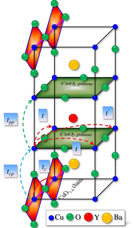
Figure 3: Crystal structure and tight-binding hopping parameters of YBCU unit cell.

Supplementary Fig. 3 presents the unit cell of YBCO crystal. The unit-cell contains two chain-layers and two CuO₂ plane layers. In order to obtain a minimum low-energy model we assume that the inter-layer electron tunneling is only active between the the two nearest neighbor layers. In doing so, we are left with a tri-layer system which consists of two CuO₂ planes and one CuO chain, while the periodic boundary conditions on infinite lattice is imposed along all three dimensions. Furthermore, the chain state does not exhibit any gap opening through out the doping range of YBCO. The plane states undergo FS reconstruction which can be captured within a commensurate spin-density wave with modulation vector ${\bm{Q}}=(\pi,\pi)$. The commensurate modulation doubles the unit cell in real-space. Using the standard Nambu notation, we define the tri-layer eigenfunction in the magnetic zone as $\Psi_{\bm{k}}^{{\dagger}}=\left[c_{p{\bm{k}}\uparrow}^{{\dagger}},~{}c_{p^{\prime}{\bm{k}}\uparrow}^{{\dagger}},~{}c_{c{\bm{k}}\uparrow}^{{\dagger}},~{}c_{p({\bm{k}}+{\bm{Q}})\downarrow}^{{\dagger}},~{}c_{p^{\prime}({\bm{k}}+{\bm{Q}})\downarrow}^{{\dagger}},~{}c_{c({\bm{k}}+{\bm{Q}})\downarrow}^{{\dagger}}\right]$. In this notation the Hamiltonian presented in the main text in Eq. 1 becomes a 6$\times$6 matrix $H=\sum_{\bm{k}}\Psi_{\bm{k}}^{{\dagger}}H_{\bm{k}}\Psi_{\bm{k}}$:

$$H_{\bm{k}}=\left(\begin{array}[]{cccccc}\ \xi_{pp{\bm{k}}}&\xi_{pp^{\prime}{\bm{k}}}&\xi_{cp{\bm{k}}}&V_{pp{\bm{k}}}&0&0\\ \xi_{pp^{\prime}{\bm{k}}}&\xi_{pp{\bm{k}}}&\xi_{cp{\bm{k}}}&0&V_{p^{\prime}p^{\prime}{\bm{k}}}&0\\ \xi_{cp{\bm{k}}}&\xi_{cp{\bm{k}}}&\xi_{cc{\bm{k}}}&0&0&0\\ V_{pp{\bm{k}}}&0&0&\xi_{pp({\bm{k}}+{\bm{Q}})}&\xi_{pp^{\prime}({\bm{k}}+{\bm{Q}})}&\xi_{cp({\bm{k}}+{\bm{Q}})}\\ 0&V_{p^{\prime}p^{\prime}{\bm{k}}}&0&\xi_{pp^{\prime}({\bm{k}}+{\bm{Q}})}&\xi_{pp({\bm{k}}+{\bm{Q}})}&\xi_{cp({\bm{k}}+{\bm{Q}})}\\ 0&0&0&\xi_{cp({\bm{k}}+{\bm{Q}})}&\xi_{cp({\bm{k}}+{\bm{Q}})}&\xi_{cc({\bm{k}}+{\bm{Q}})}\\ \end{array}\right).$$ (10)

In obtaining the non-interacting dispersions $\xi_{ij{\bm{k}}}$, we assume that Cu $d_{x^{2}-y^{2}}$ orbital contributes to the low-energy scales of present interest (as commonly used for all cuprates). The Cu $d_{x^{2}-y^{2}}$ electrons hop to their neighbors via O $p_{x,y}$ orbitals which can be taken into account within effective tight-binding formalism.markietb ; atkinson The hoping terms are depicted in supplementary Fig. 3, which gives,

$$\xi_{pp{\bm{k}}}=-2t(\phi_{x}+\phi_{y})-4t^{\prime}\phi_{x}\phi_{y}-2t^{\prime\prime}(\phi_{2x}+\phi_{2y})-\mu_{p},$$

$$\xi_{cc{\bm{k}}}=-2t_{c}\phi_{y}-\mu_{c},$$

$$\xi_{pp^{\prime}{\bm{k}}}=-2t_{pp^{\prime}}(\phi_{x}-\phi_{y})\phi_{z/4},~{}~{}~{}\xi_{cp}=-2t_{cp}\phi_{z/4},$$ (11)

where $\phi_{\alpha\mu}$=$\cos{(\alpha k_{\mu})}$ with $\mu$=$x$,$y$,$z$. $\mu_{p,c}$ are the chemical potential for the plane and chain states, respectively, which encode relative onsite energy differences and other crystal effects between the two levels. $t$,$t^{\prime}$, and $t^{\prime\prime}$ are the 1st, 2nd and 3rd nearest neighbor (NN) hopping on the 2D CuO₂ plane, $t_{c}$ is the NN hopping on the 1D chain aligned along $y$-axis, and $t_{pp^{\prime}}~{}(t_{cp})$ is the plane-plane (chain-plane) hopping along $z-$direction.

The eigenvalues for the upper 3$\times$3 interblock matrix is obtained as

$$E_{C{\bm{k}}} = \epsilon^{+}_{\bm{k}}+E_{0{\bm{k}}}$$ (12)

$$E_{A{\bm{k}}} = \epsilon^{+}_{\bm{k}}-E_{0{\bm{k}}}$$ (13)

$$E_{B{\bm{k}}} = \chi^{-}_{\bm{k}}.$$ (14)

Here subscripts ‘A’ and ‘B’ stand for the anti-bonding and bonding states created by the bi-CuO₂ layers, where ‘C’ denotes the chain state. $\epsilon^{\pm}_{\bm{k}}=(\chi^{+}_{\bm{k}}\pm\xi_{cc{\bm{k}}})/2$, $\chi^{\pm}_{\bm{k}}=\xi_{pp{\bm{k}}}\pm\xi_{pp^{\prime}{\bm{k}}}$, and $E_{0{\bm{k}}}=\sqrt{((\epsilon^{-}_{\bm{k}})^{2}+2\xi^{2}_{cp{\bm{k}}}}$. Of course, the weight of the each layers are mixed between each bands which can be determined by their corresponding eigenvectors: $u^{\pm}_{\bm{k}}=\frac{1}{2}\left[\epsilon^{-}_{\bm{k}}\pm E_{0{\bm{k}}}\right]/{\xi_{cp{\bm{k}}}}$. The eigenvalues of the full Hamiltonian can now be expressed as two split bands of the above three bands gapped by SDW order parameter $V_{ij}$DasSDW ; DDW :

$$E^{\pm}_{C{\bm{k}}} = \xi^{+}_{C{\bm{k}}}\pm\xi^{-}_{C{\bm{k}}}$$ (15)

$$E^{\pm}_{A{\bm{k}}} = \xi^{+}_{A{\bm{k}}}\pm\sqrt{\left({}^{-}\xi_{A{\bm{k}}}\right)^{2}+V_{A}^{2}}$$ (16)

$$E^{\pm}_{B{\bm{k}}} = \xi^{+}_{B{\bm{k}}}\pm\sqrt{\left(\xi^{-}_{B{\bm{k}}}\right)^{2}+V_{B}^{2}},$$ (17)

where $\xi^{\pm}_{i{\bm{k}}}=\left(E_{A{\bm{k}}}\pm E_{A{\bm{k}}}\right)/2$ and the self-consistent order parameters $V_{i}$ are given below. The eigenvectors for the final eigenstates given above can be represented in terms of SDW coherence factors:

$$\alpha^{2}_{i{\bm{k}}} = \frac{1}{2}\left(1+\xi^{-}_{i{\bm{k}}}/\sqrt{\left(\xi^{-}_{i{\bm{k}}}\right)^{2}+V_{i}^{2}}\right),$$

$$\beta^{2}_{i{\bm{k}}} = 1-\alpha^{2}_{i{\bm{k}}}.$$ (18)

Here $i=A,B,C$. Due to the absence of any gap opening in the chain state, $\alpha^{2}_{C{\bm{k}}}=1$ and $\beta^{2}_{C{\bm{k}}}=0$ at all momentum. With the definitions of the eigenstates and the coherence factors, we construct the final unitary matrix $\hat{U}_{\bm{k}}$ that ultimately diagonalize the total Hamiltoanin given above in Eq.

$${\hat{U}}_{\bm{k}}=\left(\begin{array}[]{cccccc}\ u^{+}_{\bm{k}}&u^{-}_{\bm{k}}\alpha_{A{\bm{k}}}&-\alpha_{B{\bm{k}}}&0&-u^{-}_{\bm{k}}\beta_{A{\bm{k}}}&\beta_{B{\bm{k}}}\\ u^{-}_{\bm{k}}\alpha_{A{\bm{k}}}&u^{+}_{\bm{k}}\alpha_{A{\bm{k}}}&\alpha_{B{\bm{k}}}&0&-u^{+}_{\bm{k}}\beta_{A{\bm{k}}}&-\beta_{B{\bm{k}}}\\ -\alpha_{B{\bm{k}}}&\alpha_{B{\bm{k}}}&0&0&-\beta_{B{\bm{k}}}&0\\ 0&0&0&0&0&0\\ u^{-}_{\bm{k}}\beta_{A{\bm{k}}}&u^{+}_{\bm{k}}\beta_{A{\bm{k}}}&\beta_{B{\bm{k}}}&0&u^{+}_{\bm{k}}\alpha_{A{\bm{k}}}&\alpha_{B{\bm{k}}}\\ -\beta_{B{\bm{k}}}&\beta_{B{\bm{k}}}&0&0&\alpha_{B{\bm{k}}}&0\end{array}\right).$$ (25)

(26)

The self-consistent order parameters are defined as $V_{A}=US_{A}$ and $V_{B}=US_{B}$ (and $V_{C}=0$), where $U$ is the onsite Hubbard interaction which is kept to be same for both CuO₂ planes. $S_{A/B}$ are the two order parameters, $p$ is the dopin concentration which are evaluated by solving the following two self-consistent equations:

$$p = 2-\frac{1}{N}\sum_{{\bm{k}},i=1,2,\sigma}\left\langle c_{i{\bm{k}}\sigma}^{{\dagger}}c_{i{\bm{k}}\sigma}\right\rangle$$ (27)

$$= 2-\frac{1}{N}\sum_{{\bm{k}},i}\hat{U}_{ii{\bm{k}}}\hat{U}_{ii{\bm{k}}}^{{\dagger}}f(E_{i{\bm{k}}}),$$

$$S_{i} = \frac{1}{2}\left(n_{i\uparrow}-n_{i\downarrow}\right)$$ (28)

$$= \frac{1}{2N}\sum_{\bm{k}}\left[\left\langle c_{i({\bm{k}}+{\bm{Q}})\uparrow}^{{\dagger}}c_{i{\bm{k}}\uparrow}\right\rangle-\left\langle c_{i({\bm{k}}+{\bm{Q}})\downarrow}^{{\dagger}}c_{i{\bm{k}}\downarrow}\right\rangle\right]$$

$$= \frac{1}{2N}\sum_{{\bm{k}},j}\hat{U}_{ij{\bm{k}}}\hat{U}_{ji{\bm{k}}}^{{\dagger}}f(E_{j{\bm{k}}}),$$

where $f$ is the Fermi function and $E_{j}$ are the eigenstates listed in Eq. 16-17 where indices $i$=A,B and $j$=1-6. $n_{i\uparrow}$ is the number of up-spin on the $i^{th}$ layer defined as $\left\langle c_{i({\bm{k}}+{\bm{Q}})\uparrow}^{{\dagger}}c_{i{\bm{k}}\uparrow}\right\rangle$, where the thermal average is taken over the whole Brillouin zone.

Tight-binding parameters and self-consistent order parameters

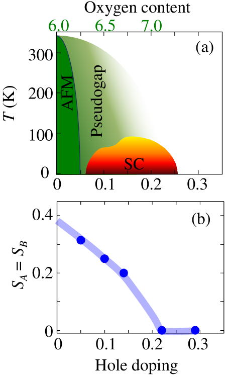
Figure 4: (a) Schematic phase diagram of cuprate. (b) The doping dependence of self-consistently evaluated order parameter $S$ (defined in the text).

We find that the tight-binding parameters that give a good description of the FS, in agreement with ARPES and first-principle band-structure areatkinson : $(t,t^{\prime},t^{\prime\prime},t^{\prime\prime},t_{c},t_{pp^{\prime}},t_{cp})$=(0.38, 0.0684,0.095,0.25,-0.01,-0.0075) eV. We have kept $\mu_{c}=-0.87$ eV to be doping independent, while $\mu_{p}$ is computed self-consistently. The band structure fitting is done at the overdoped sample of $p=0.29$, shown in Fig. 1 in the main text.

The calculation of self-consistency is carried out in the following steps. At a given doping $p$ and onsite Hubbard $U$=1.59 eV, we start our self-consistent cycle with an initial guess of chemical potential $\mu_{p}$ and order parameters $S_{A/B}$, and calculate doping $p$ and $S_{A/B}$ by solving Eqs. (1) to (12) at $T=0$. We iterate the entire loop until the self-consistent values of doping $p$, and order parameters $S_{A/B}$ converges. For the overdoped sample of $p=0.29$, we get $S_{A/B}=0$ and $\mu_{p}$=-0.54 eV. At an extreme underdoped samples of $p=0.05$ at which ARPES data are available for fitting in Fig. 1, we get $S_{A}(T=0)\approx S_{B}(T=0)=0.3145$ and $\mu_{p}=-0.4$. At two dopings at which Fig. 2 is obtained in the main text, we find $S_{A}(T=0)\approx S_{B}(T=0)=0.25$ and $\mu_{p}$=-0.41 at $T$=0 to -0.43 eV at $T=55$ K for $p$=0.10, and $S_{A}(T=0)\approx S_{B}(T=0)=0.22$ and $\mu_{p}$=-0.38 at $T$=0 to -0.41 eV at $T=55$ K for $p$=0.14. The results are plotted in supplementary Fig. 4(b), and compared with the schematic phase diagram of YBCO in Fig. 1(a). Note that the temperature dependence of the order parameters is phenomenologically assumed as $S_{i}=S_{i}(0)\sqrt{1-T/T_{s}}$, where $T_{s}=55$ K is the SDW transition temperature.Sachdev_stripe ; Ts

II Details of Hall and Nernst coefficient calculations.

The Nernst effect experiments measure the transverse electric field response of a system to a combination set-up of an externally-imposed temperature gradient and an orthogonal magnetic field. The Nernst effect depends sensitively on anisotropies in the band structure. Similarly, the Hall effect is a powerful probe of the Fermi surface of a metal because of its sensitivity to the sign of charge carriers, which distinguishes between electrons and holes. These two probes have recently gained much attention in the context of cuprates, since they demonstrate very unusual behavior in the underdoped region when the pseudogap sets in. Apart from the superconducting fluctuation origin of enhanced Nernst effect in cuprates,Nernst_prepairing purely quasiparticle picture is extensively proposed in various contexts.ambipolar ; Sachdev_SDW ; Sachdev_stripe ; DDW_Nernst The quasiparticle Nernst effect has been studied on the basis of the linearized Boltzmann equation in the relaxation-time approximation. This is a reliable approach if the scattering rate is isotropic, since then the neglected ‘scattering-in’ contributions average out to zero.

We start from the semiclassical Boltzmann transport equation for quasiparticles (charge $e$) in a weak magnetic field ${\bm{B}}$, driven out of equilibrium by a spatially uniform electric field ${\bm{E}}$ and temperature gradient $\nabla T$. If we linearize the deviation of the fermion distribution function from its equilibrium state $f(\xi_{\bm{k}})$ in both ${\bm{E}}$ and $\nabla T$ as $f^{\prime}(\xi_{\bm{k}})=f+g_{\bm{k}}$, then the Boltzmann equationNernst_QSH becomes:

$$V_{\bm{k}}\left(-\frac{\partial f(\xi_{\bm{k}})}{\partial\xi_{\bm{k}}}\right)-\Omega^{0}_{\bm{k}}g_{\bm{k}}=\sum_{{\bm{k}}^{\prime}}Q_{{\bm{k}},{\bm{k}}^{\prime}}\left(g_{\bm{k}}-g_{{\bm{k}}^{\prime}}\right)$$ (29)

$$V_{\bm{k}}={\bm{v}}_{\bm{k}}\cdot\left(-e{\bm{E}}-\xi_{\bm{k}}\frac{\nabla T}{T}\right)$$ (30)

$$\Omega_{\bm{k}}=-\frac{e}{\hbar c}\left({\bm{v}}_{\bm{k}}\times{\bm{B}}\right)\cdot\nabla_{\bm{k}}.$$ (31)

Here $\xi_{\bm{k}}$ is the quasiparticle state whose velocity is ${\bm{v}}_{\bm{k}}=\hbar^{-1}\nabla_{\bm{k}}\xi_{\bm{k}}$. The band index and the eigenvectors are implicit to the quasiparticle states in the above equations. $Q_{{\bm{k}},{\bm{k}}^{\prime}}$ is the scattering matrix-element for incoming state $\sum_{{\bm{k}}^{\prime}}Q_{{\bm{k}},{\bm{k}}^{\prime}}g_{{\bm{k}}^{\prime}}$ and outgoing state $\sum_{{\bm{k}}^{\prime}}Q_{{\bm{k}},{\bm{k}}^{\prime}}g_{{\bm{k}}}$. For the present DC transport property, we assume the elastic scattering with $Q_{{\bm{k}},{\bm{k}}^{\prime}}=\delta(\xi_{\bm{k}}-\xi_{{\bm{k}}^{\prime}})q_{{\bm{k}},{\bm{k}}^{\prime}}$. Furthermore, we impose the standard relaxation-time approximation,RelaxA which implies that the system has enough time to loose its memory, i. e. scattering-in term is negligible. In that case, the scattering rate is governed is entirely governed by the out-going state as $\frac{g_{\bm{k}}}{\tau_{\bm{k}}}=g_{\bm{k}}\sum_{{\bm{k}}^{\prime}}Q_{{\bm{k}},{\bm{k}}^{\prime}}$, while relating its momentum dependence:

$$\frac{1}{\tau_{\bm{k}}}=\sum_{{\bm{k}}^{\prime}}{\hat{Q}}_{{\bm{k}},{\bm{k}}^{\prime}}=N_{0}\left\langle q_{{\bm{k}},{\bm{k}}^{\prime}}\right\rangle_{FS}.$$ (32)

Within this approximation Eq. 29-31 becomes

$$g_{\bm{k}}=\Omega_{\bm{k}}^{-1}V_{\bm{k}}\left(-\frac{\partial f(\xi_{\bm{k}})}{\partial\xi_{\bm{k}}}\right)$$ (33)

$$V_{\bm{k}}={\bm{v}}_{\bm{k}}\cdot\left(-e{\bm{E}}-\xi_{\bm{k}}\frac{\nabla T}{T}\right)$$ (34)

$$\Omega_{\bm{k}}=-\left[\frac{e}{\hbar c}\left({\bm{v}}_{\bm{k}}\times{\bm{B}}\right)\cdot\nabla_{\bm{k}}+\frac{1}{\tau_{\bm{k}}}\right].$$ (35)

It is now convenient to introduce the band index $n$:

$$g_{n{\bm{k}}}=\Omega_{n\bm{k}}^{-1}V_{n\bm{k}}\left(-\frac{\partial f(\xi_{n\bm{k}})}{\partial\xi_{n\bm{k}}}\right),$$ (36)

From Eq. 36, the net electrical, ${\bm{J}}$, and thermal current densities, ${\bm{Q}}$, that flow on the $i^{t}h$-layer (or orbital) can be calculated as from the diagonal term of the following matrix

$${\bm{J}}^{ij} = -2e\sum_{{\bm{k}},n}M_{n}^{ij}{\bm{v}}_{n\bm{k}}g_{n\bm{k}}$$ (37)

$${\bm{Q}}^{ij} = 2\sum_{{\bm{k}},n}M_{n}^{ij}{\bm{v}}_{n\bm{k}}\xi_{n{\bm{k}}}g_{n\bm{k}},$$ (38)

where $M$ is the matrix-element:

$$M_{n}^{ij}({\bm{k}})=\psi_{n}^{i}({\bm{k}})\psi_{n}^{j{\dagger}}({\bm{k}}).$$ (39)

In Eq. 37, we project the densities from its band basis $n$ (a band index is implicit on both sides of Eq. 34) to the layer indices, $i,j$. The factor ‘2’ introduced in Eqs. 37-38 to count spin-degeneracy.

Linear response theory: The interplay of electrical and thermal effects necessarily implies two conductivity tensors $\hat{\sigma}$, $\hat{\alpha}$, which relate charge current ${\bm{J}}$ to electric field, ${\bm{E}}$ and thermal gradient, $\nabla T$ vectors:

$${\bm{J}}^{ij}=\hat{\sigma}^{ij}{\bm{E}}-\hat{\alpha}^{ij}\nabla T$$ (40)

The Nernst response is defined as the electricalfield induced by a thermal gradient in the absence of an electrical current, and is given in linear response by the relation ${\bm{E}}=-\hat{\theta}\nabla T$. In absence of charge current (i.e. when ${\bm{J}}$=0), Eq. (6) yields:

$${\bm{E}}=(\hat{\sigma}^{ij})^{-1}\hat{\alpha}^{ij}\nabla T=-\hat{\theta}^{ij}\nabla T,$$ (41)

where Hall resistance, $\hat{\rho}$=$\hat{\sigma}^{-1}$, and the Nernst coefficient, ${\nu}$=$\hat{\theta}/B$, are measured independently via transport probes by setting a weak magnetic field ${\bm{B}}$=$B\hat{z}$ along the $c$-axis of the lattice.HallEP ; Nernst_data In Eq. 40 and 41, the layer indices $i,j$ run on both sides. From Eqs. 34,37, 40, we easily deduce that

$$\hat{\sigma}^{ij}_{\mu\nu} = 2\sum_{{\bm{k}},n}M_{n}^{ij}{\bm{v}}^{\mu}_{n\bm{k}}\Omega_{n\bm{k}}^{-1}\left(\frac{\partial V^{\nu}_{n\bm{k}}}{\partial{\bm{E}}}\right)\left(-\frac{\partial f(\xi_{n\bm{k}})}{\partial\xi_{n\bm{k}}}\right)=\frac{\beta e^{2}}{2}\sum_{{\bm{k}},n}M_{n{\bm{k}}}^{ij}v^{\mu}_{n{\bm{k}}}\Omega_{n{\bm{k}}}^{-1}v^{\nu}_{n{\bm{k}}}{\rm sech}^{2}\left(\frac{\beta E_{n{\bm{k}}}}{2}\right)$$ (42)

$$\hat{\alpha}^{ij}_{\mu\nu} = 2\sum_{{\bm{k}},n}M_{n}^{ij}{\bm{v}}^{\mu}_{n\bm{k}}\Omega_{n\bm{k}}^{-1}\left(\frac{\partial V^{\nu}_{n\bm{k}}}{\partial(-\nabla T)}\right)\left(-\frac{\partial f(\xi_{n\bm{k}})}{\partial\xi_{n\bm{k}}}\right)=-\frac{\beta^{2}e}{2}\sum_{{\bm{k}},n}M_{n{\bm{k}}}^{ij}v^{\mu}_{n{\bm{k}}}\Omega_{n{\bm{k}}}^{-1}v^{\nu}_{n{\bm{k}}}E_{n{\bm{k}}}{\rm sech}^{2}\left(\frac{\beta E_{n{\bm{k}}}}{2}\right)$$ (43)

where we have used the identity $\left(-\frac{\partial f(\xi_{n\bm{k}})}{\partial\xi_{n\bm{k}}}\right)=\frac{\beta}{4}{\rm sech}^{2}\left(\frac{\beta E_{n{\bm{k}}}}{2}\right)$. In the usual manner, the differential operator $\Omega_{n\bm{k}}^{-1}$ can be arranged as a perturbative expansion in the magnetic field ${\bm{B}}$Sachdev_stripe ; RelaxA in order to obtain transport coefficients that do not depend on ${\bm{B}}$. For this purpose we define $\Omega_{n\bm{k}}$= $\Upsilon_{n\bm{k}}$+$\Lambda_{n\bm{k}}$ (Eq. 31), where $\Upsilon_{n\bm{k}}=1/\tau_{n\bm{k}}$ and $\Lambda_{n\bm{k}}$ is the rest. Then

$$\Omega_{n\bm{k}}^{-1}=\Upsilon_{n\bm{k}}^{-1}-\Upsilon_{n\bm{k}}^{-1}\Lambda_{n\bm{k}}\Upsilon_{n\bm{k}}^{-1}+\mathcal{O}(B^{2}).$$ (44)

The diagonal entries in Eq. 43 (in the $\mu,\nu$ basis, not in the $i,j$ basis) are obtained from the zeroth order in ${\bm{B}}$ in Eq. 44, while the lowest-order contribution to the off-diagonal coefficients arises from the linear order in ${\bm{B}}$ in the expansion of Eq. 44. To this accuracy, the expressions Eq. 43 can be simplified in form of the expressions

$$\hat{\sigma}^{ij}_{\mu\mu} = \frac{\beta e^{2}}{2}\sum_{{\bm{k}},n}M_{n{\bm{k}}}^{ij}(v^{\mu}_{n{\bm{k}}})^{2}\tau_{0}{\rm sech}^{2}\left(\frac{\beta E_{n{\bm{k}}}}{2}\right)$$ (45)

$$\hat{\sigma}^{ij}_{\mu\neq\nu} = \frac{\beta e^{3}B}{2\hbar c}\sum_{{\bm{k}},n}M_{n{\bm{k}}}^{ij}v^{\mu}_{n{\bm{k}}}\tau_{0}^{2}\left[v^{\nu}_{n{\bm{k}}}\frac{\partial v^{\nu}_{n{\bm{k}}}}{\partial{\bm{k}}^{\mu}}-v^{\mu}_{n{\bm{k}}}\frac{\partial v^{\nu}_{n{\bm{k}}}}{\partial{\bm{k}}^{\nu}}\right]{\rm sech}^{2}\left(\frac{\beta E_{n{\bm{k}}}}{2}\right)$$ (46)

$$\hat{\alpha}^{ij}_{\mu\mu} = -\frac{\beta^{2}e}{2}\sum_{{\bm{k}},n}M_{n{\bm{k}}}^{ij}(v^{\mu}_{n{\bm{k}}})^{2}\tau_{0}E_{n{\bm{k}}}{\rm sech}^{2}\left(\frac{\beta E_{n{\bm{k}}}}{2}\right)$$ (47)

$$\hat{\alpha}^{ij}_{\mu\neq\nu} = -\frac{\beta^{2}e^{2}B}{2\hbar c}\sum_{{\bm{k}},n}M_{n{\bm{k}}}^{ij}v^{\mu}_{n{\bm{k}}}\tau^{2}_{0}\left[v^{\nu}_{n{\bm{k}}}\frac{\partial v^{\nu}_{n{\bm{k}}}}{\partial{\bm{k}}^{\mu}}-v^{\mu}_{n{\bm{k}}}\frac{\partial v^{\nu}_{n{\bm{k}}}}{\partial{\bm{k}}^{\nu}}\right]E_{n{\bm{k}}}{\rm sech}^{2}\left(\frac{\beta E_{n{\bm{k}}}}{2}\right)$$ (48)

In a simplest model, we assume a momentum and temperature independent value of relaxation time $\tau_{\bm{k}}=\tau_{0}$. A temperature dependent value of $\tau_{0}$ can improve the results, especially for the Nernst signal, however, with this simplest form, we are able to capture the salient features of both Hall coefficient and Nernst coefficient. The results in the main text are normalized to the constant value of $B$ and $\tau_{0}$. The above expressions matches exactly with the one proposed earlier for various form of density wave order,Sachdev_stripe ; Sachdev_SDW ; DDW_Nernst except the matrix-element terms. It is important to note that, if no other crystal symmetry is broken, then the Mott relation $\nu_{xy}=-\nu_{yx}$ for Nernst coefficient can be recovered from the Boltzmann theory.Vojta This implies that the choice of sign convention for the Nernst effect is arbitrary. To faciliate direct comparison, we have taken the same sign for $|\nu_{a}|$ and $|\nu_{b}|$.

References

- (1) R. S. Markiewicz et al. Phys. Rev. B 72, 054519 (2007).
- (2) W. A. Atkinson, Phys. Rev. B 59, 3377 (1999).
- (3) T. Das, R. S. Markiewicz, and A. Bansil, Phys. Rev. B 77, 134516 (2008).
- (4) S. Chakravarty, and H.Y. Kee. Proc. Nat. Acad. Sci. USA 105, 8835 (2008).
- (5) A. Hackl, M. Vojta, and S. Sachdev, Phys. Rev. B 81, 045102 (2010).
- (6) N. Ichikawa et al., Phys. Rev. Lett. 85, 1738 (2000).
- (7) K. Behnia, J. Phys. Condens. Matter 21, 113101 (2009).
- (8) V. Oganesyan, and I. Ussishkin, Phys. Rev. B 70, 054503 (2004).
- (9) A. Hackl, and S. Sachdev, Phys. Rev. B 79, 235124 (2009).
- (10) C. Zhang, S. Tewari, and S. Chakravarty, Phys. Rev. B 81, 104517 (2010).
- (11) D.I. Pikulin, C.Y. Hou, and C.W.J. Beenakker, hys.Rev. B 84, 035133 (2011).
- (12) J. M. Ziman, Oxford University Press, Oxford (1960).
- (13) D. LeBoeuf et al., Nature 450, 533-536 (2007).
- (14) J. Chang et al. Phys. Rev. B 84, 014507 (2011).
- (15) A. Hackl, and M. Vojta, Phys. Rev. B 80, 220514(R) (2009).