Template RR Lyrae ${\rm H\alpha}$, ${\rm H\beta}$, and ${\rm H\gamma}$ velocity curves

Abstract

We present template radial velocity curves of $ab$-type RR Lyrae stars constructed from high-precision measurements of ${\rm H\alpha}$, ${\rm H\beta}$, and ${\rm H\gamma}$ lines. Amplitude correlations between the Balmer line velocity curves, Johnson $V$-band, and SDSS $g$- and $r$-band light curves are also derived. Compared to previous methods, these templates and derived correlations reduce the uncertainty in measured systemic (center-of-mass) velocities of RR Lyrae stars by up to 15 ${\rm km~{}s}^{-1}$, and will be of particular interest to wide-area spectroscopic surveys such as the Sloan Digital Sky Survey (SDSS) and LAMOST Experiment for Galactic Understanding and Exploration (LEGUE).

1 Introduction

RR Lyrae stars are old ($\gtrsim 9$ Gyr), low-mass ($\sim 0.7M_{\sun}$), pulsating stars ($V$-band amplitudes of $A_{V}\sim 1$ mag and periods of $\sim 0.6$ days) that reside in the instability strip of the horizontal branch (Smith, 1995). They are valuable tracers of old stellar populations and have recently been used to map the Galactic halo structure (i.e., its stellar number density profile) and substructure (e.g., tidal streams and halo overdensities; Vivas et al. 2001, Keller et al. 2008, Miceli et al. 2008, Watkins et al. 2009, Sesar et al. 2010a).

While the spatial distribution of RR Lyrae stars is a powerful indicator of candidate halo substructures (e.g., Fig. 11 of Sesar et al. 2010a), it does not always reveal the full nature of halo substructures. For example, the Pisces Overdensity, a spatial group of about a dozen RR Lyrae stars at $\sim 80$ kpc from the Sun (clump “J” in Sesar et al. 2007; Watkins et al. 2009), was initially suspected to be a part of a tidal stream (Sesar et al., 2010a). However, spectroscopic observations by Kollmeier et al. (2009) and Sesar et al. (2010b) have revealed that the overdensity actually consists of two velocity groups; one moving towards and the other one moving away from the Galactic center. This result suggests that the Pisces Overdensity may be a pile-up of tidal debris near the orbital turn-around point of a now-disrupted progenitor (which was, most likely, a dwarf spheroidal galaxy; Sesar et al. 2010b).

The Kollmeier et al. (2009) and Sesar et al. (2010b) findings underline the importance of obtaining kinematic data on candidate halo substructures; the nature and interpretation of a halo substructure can quickly change once kinematic data become available. Yet, relative to photometric data, which is abundant in this era of wide-area and multi-epoch surveys, spectroscopic observations are more scarce and may be considered as more “expensive” in terms of telescope time. Obtaining the kinematic information for variable stars, such as RR Lyrae stars, is even more complicated as one needs to subtract the velocity due to pulsations to get the center-of-mass (hereafter, systemic) velocity.

There are two approaches to this problem of determining the systemic velocity of RR Lyrae stars. In the first approach, one tries to observe RR Lyrae stars at a particular point during a pulsation period when the observed radial velocity is presumed to be equal to the star’s systemic velocity (usually at ${\rm phase\sim 0.5\pm 0.1}$, see Section 6). Unfortunately, sometimes it is very difficult to schedule observations to target this point (e.g., when executing observations in queue or service mode). In addition, RR Lyrae stars are dimmer near phase 0.5 ($\sim 0.3-0.5$ mag compared to maximum light at phase of 0), and thus require longer exposures to reach the same signal-to-noise ratio. The danger of longer exposures is blurring of spectral lines due to pulsations, which in turn decreases the precision of radial velocity measurements.

In the second approach, one assumes a certain model (a template) that describes the radial velocity due to pulsations as a function of pulsation phase. The amplitude, $A_{rv}$, of the radial velocity curve template (hereafter, template) is then scaled using a correlation between the amplitudes of velocity curves and light curves. The velocity at any phase can then be easily read-out once the scaled template is matched to one or several radial velocity observations taken at known phases. An example of such a template and an equation relating velocity and light curve amplitudes is provided by Liu (1991) (see his Equation 1). The advantage of this approach is that the systemic velocity can be estimated using radial velocities obtained in phases different from phase of 0.5.

Unfortunately, Liu’s template and his velocity vs. light curve amplitude relation are not really suitable for estimating systemic velocities of distant (i.e., faint) RR Lyrae stars because they were derived from measurements of metallic lines and should only be used with measurements of such lines. This is a problem since measuring radial velocities using metallic lines requires high-resolution spectroscopy ($R\gtrsim 10000$), and obtaining quality, high-resolution spectra of faint ($V>18$) stars with exposures that are a small fraction of the pulsation period ($\lesssim 10\%$ to avoid spectral blurring) is virtually impossible with today’s facilities.

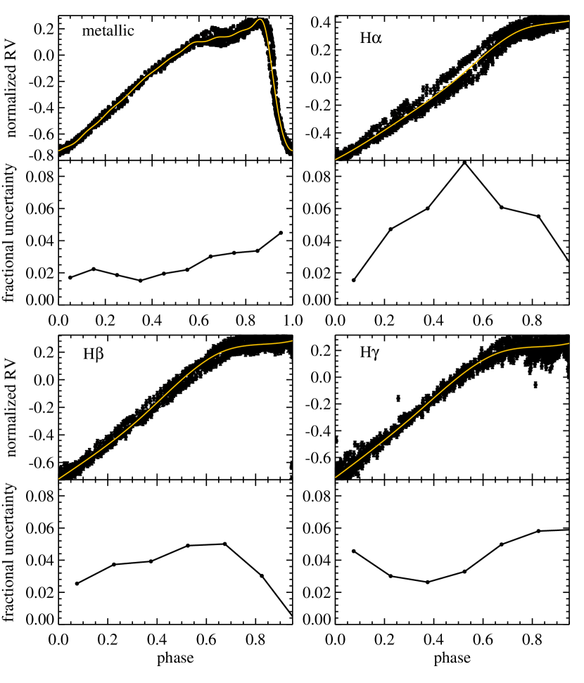
Figure 1: Normalized and phased radial velocity curves obtained from measurements of metallic lines (top left panel), ${\rm H\alpha}$ line (top right panel), ${\rm H\beta}$ line (bottom left panel), and ${\rm H\gamma}$ line (bottom right panel). In each panel, the solid line shows a B-spline curve interpolated through normalized radial velocities (i.e., the template radial velocity curve). The template and the normalized radial velocities are offset so the velocity at phase 0.5 (the phase at which the radial velocity is presumed to be equal to the systemic velocity, see Section 6) is equal to 0. The connected points in the bottom plot of each panel show the rms scatter in the template velocity curve (in units of ${\rm A_{rv}}$), and represent the uncertainty in the shape of the template.

Instead of using weak metallic lines, a more practical choice would be to use strong Balmer lines (${\rm H\alpha}$ to ${\rm H\delta}$), which can be observed with more widely available low-resolution ($R\sim 1500$) spectrographs. However, Liu’s template and his velocity vs. light curve amplitude relation cannot be used with measurements of Balmer lines because the Balmer line velocity curves have a different shape and amplitude than the velocity curve of metallic lines (Oke, 1962). A method adopted by many studies (e.g., Hawley & Barnes 1985; Layden 1994; Vivas et al. 2005; Prior et al. 2009; Sesar et al. 2010b, 2012) is to use the radial velocity curve of RR Lyrae star X Ari measured from the ${\rm H\gamma}$ line by Oke (1966). This is not an ideal solution because the velocity curve amplitude of X Ari ($A_{rv}\sim 85$ ${\rm km~{}s}^{-1}$, see Figure 1 of Oke 1966) will likely not be similar to the velocity curve amplitude of some other star with a different $V$-band light curve amplitude (${\rm A_{V}}$). The consequence of using an inadequate model for radial velocities is a more uncertain estimate of the systemic velocity.

The ability to precisely measure systemic velocities of RR Lyrae stars is very important as it may help with various Galactic studies, such as identifying halo substructures using kinematics (e.g., the Pisces Overdensity groups), discerning the nature of progenitors of halo substructures (e.g., globular cluster vs. a dwarf spheroidal galaxy), and constraining orbits of halo substructures (e.g., the Virgo Overdensity; Casetti-Dinescu et al. 2009; Carlin et al. 2012). In addition, obtaining precise systemic velocities of RR Lyrae stars using one or two measurements would be beneficial to spectroscopic surveys such as the LAMOST Experiment for Galactic Understanding and Exploration (LEGUE; Deng et al. 2012), which may observe several thousands of RR Lyrae stars within 30 kpc of the Sun, and which plan to study the kinematics and structure of the Galactic halo.

In this paper, we use high-precision measurements of ${\rm H\alpha}$, ${\rm H\beta}$, and ${\rm H\gamma}$ lines of six field $ab$-type RR Lyrae stars to first construct template radial velocity curves (Section 3). We then derive correlations between amplitudes of Balmer line velocity curves and light curves observed in Johnson $V$-band (Section 4) or SDSS $g$- and $r$-bands (Section 5). The systemic velocity of RR Lyrae stars and its uncertainty are defined in Section 6, and the results, along with implications for surveys such as LINEAR, PTF, LEGUE, and LSST, are discussed in Section 7.

2 Data set

The sample of stars used in the construction of velocity templates consists of 6 field RR Lyrae type $ab$ stars (see Table 1) that were observed between 2006 and 2009 by George W. Preston with the echelle spectrograph of the du Pont 2.5 m telescope at the Las Campanas Observatory. The stars have $V$-band light curve amplitudes (${\rm A_{V}}$) ranging from 0.64 mag (Z Mic) to 1.13 mag (RV Oct), as measured by the All Sky Automated Survey (ASAS; Pojmański 1997). According to Szczygiel & Fabrycky (2007), three of the stars in this sample exhibit the Blazhko effect in their light curves (Blazhko, 1907; Smith, 1995).

The observations, data reduction, and measurement of radial velocities are described in detail in For et al. (2011). The data, kindly provided to us by George W. Preston (private communication), consist of radial velocity measurements obtained using metallic and Balmer lines (${\rm H\alpha}$, ${\rm H\beta}$, and ${\rm H\gamma}$). The formal random error is $\sim 0.5$ ${\rm km~{}s}^{-1}$ for radial velocities obtained using metallic lines, and $\sim 3$ ${\rm km~{}s}^{-1}$ for radial velocities obtained using Balmer lines. In addition, systematic errors of $\sim 1$ to 2 ${\rm km~{}s}^{-1}$ may also be present. The phase of each observation was calculated using periods and epochs of maximum light listed in Table 5 of For et al. (2011), with the time of maximum light corresponding to phase of 0. The number of observations per star ranges from about 100 (DT Hya) to about 240 (XZ Aps).

3 Construction of velocity templates

We start by normalizing radial velocities to the range ${\rm[0,1]}$. The normalization is done on a per star basis using

$$rv_{norm}=\frac{rv-rv_{min}}{rv_{max}-rv_{min}},$$ (1)

where $rv_{min}$ and $rv_{max}$ are, respectively, the lowest and highest radial velocity determined after discarding the top and bottom 1% of radial velocities of that star. The normalized velocities from all stars are then combined and a cubic B-spline is interpolated through the data. The normalized, phased, and combined radial velocities are shown in Figure 1 (top plots in each panel). The velocities and the interpolated B-spline (the template) are offset so the velocity at phase 0.5 (the phase at which the radial velocity is presumed to be equal to the systemic velocity) is equal to 0. The templates are provided in the supplementary data available in the electronic edition of the journal and at http://www.astro.caltech.edu/~bsesar/RVtemplates.tar.gz.

Note that the templates of Balmer line velocity curves do not cover the full range of phases, but end at phase of 0.95. Due to a rapid change in velocities of Balmer lines between phases of 0.95 and 1.0, we were not able to properly model the entire velocity curve with a single cubic spline. We do not consider this to be a major problem from an observational point of view because the velocities measured from Balmer lines between phases of 0.9 and 1.0 are in general more uncertain, mainly due to increased spectral blurring (i.e., due to a rapid change in velocity as a function of time), and are not very useful.

The interpolated cubic B-spline defines the average shape of the radial velocity curve. To estimate the uncertainty in this average shape, we calculate the root-mean-square (hereafter, rms) scatter around the template and plot its dependence on phase in bottom plots in each panel of Figure 1. The shape of the ${\rm H\alpha}$ template is most uncertain, with an rms scatter of $\sim 10\%$ of ${\rm A_{rv}}$ at phase of about 0.55 ($\sim 10$ ${\rm km~{}s}^{-1}$ for a RR Lyrae star with ${\rm A_{V}=1.0}$ mag). The shape of the metallic lines template curve is the least uncertain ($\sim 3\%$ of ${\rm A_{rv}}$), followed by ${\rm H\gamma}$ and ${\rm H\beta}$ template curves ($\sim 3\%$ to $4\%$ of ${\rm A_{rv}}$ or $\sim 4$ ${\rm km~{}s}^{-1}$ for a RR Lyrae star with ${\rm A_{V}=1.0}$ mag).

4 ${\rm A_{rv}}$ vs. ${\rm A_{V}}$ correlations

Having defined average velocity curves (templates), we now fit templates to observed radial velocities of each star to determine the amplitudes of metallic and Balmer lines velocity curves (${\rm A_{rv}}$). The best-fit amplitudes are listed in Table 1, and are plotted versus $V$-band amplitudes in Figure 2.

As Liu (1991) (hereafter, L91) first noted, there is a tight correlation between the amplitudes of metallic lines velocity curves and $V$-band light curves. We also see a similar correlation, but for velocity curves measured from Balmer lines. Following L91, we do an unweighted, linear least-squares fit to velocity amplitudes as a function of the $V$-band light curve amplitudes and find:

$$A_{rv}^{met}=25.6(\pm 2.5)A_{V}+35.0(\pm 2.3),\,\sigma_{fit}=2.4\,km\,s^{-1}$$ (2)

$$A_{rv}^{H\alpha}=35.6(\pm 2.5)A_{V}+78.2(\pm 2.4),\,\sigma_{fit}=3.4\,km\,s^{-1}$$ (3)

$$A_{rv}^{H\beta}=42.1(\pm 2.5)A_{V}+51.1(\pm 2.4),\,\sigma_{fit}=3.0\,km\,s^{-1}$$ (4)

$$A_{rv}^{H\gamma}=46.1(\pm 2.5)A_{V}+38.5(\pm 2.4),\,\sigma_{fit}=2.8\,km\,s^{-1},$$ (5)

where ${\rm\sigma_{fit}}$ is the rms scatter of the best fit.

In the top left panel of Figure 2, we compare our best-fit for metallic lines (Equation 2) to

$$A_{rv}^{L91}=\frac{40.5A_{V}+42.7}{1.37},$$ (6)

which is the best-fit for metallic lines obtained by L91 (his Equation 1) scaled by the so-called “projection factor” $p=1.37$. Equation 1 of L91 needs to be scaled because L91 uses pulsation velocities, which are related to observed radial velocities as $v_{obs}=v_{puls}/p$ (see Liu’s Equation 2). The projection factor was estimated as the average ratio of velocities calculated using Liu’s Equation 1 and metallic ${\rm A_{rv}}$ values listed in Table 1. The estimated projection factor $p=1.37$ is in the range of values listed by L91 and Kovács (2003) (1.31 to 1.37). In conclusion, the scaled L91 fit and our fit are remarkably similar (within $\sim 2.5$ ${\rm km~{}s}^{-1}$ of rms scatter), even though Liu’s sample has more stars and spans a much greater range of $V$-band amplitudes than our sample (Liu’s sample extends up to ${\rm A_{V}\sim 1.3}$ mag).

Figure 2 shows that for a fixed $V$-band amplitude, each of the Balmer lines studied here has a different velocity curve amplitude. This suggests that, in theory, the most precise systemic velocity may be obtained by averaging systemic velocities which are estimated from radial velocities measured from individual Balmer lines. However, in some cases (e.g., for faint stars), it may make more sense to measure radial velocities by cross-correlating more than one Balmer line with a reference spectrum. Due to the fact that Balmer line velocity curves have different shapes and amplitudes, we expect that such measurements may be more uncertain.

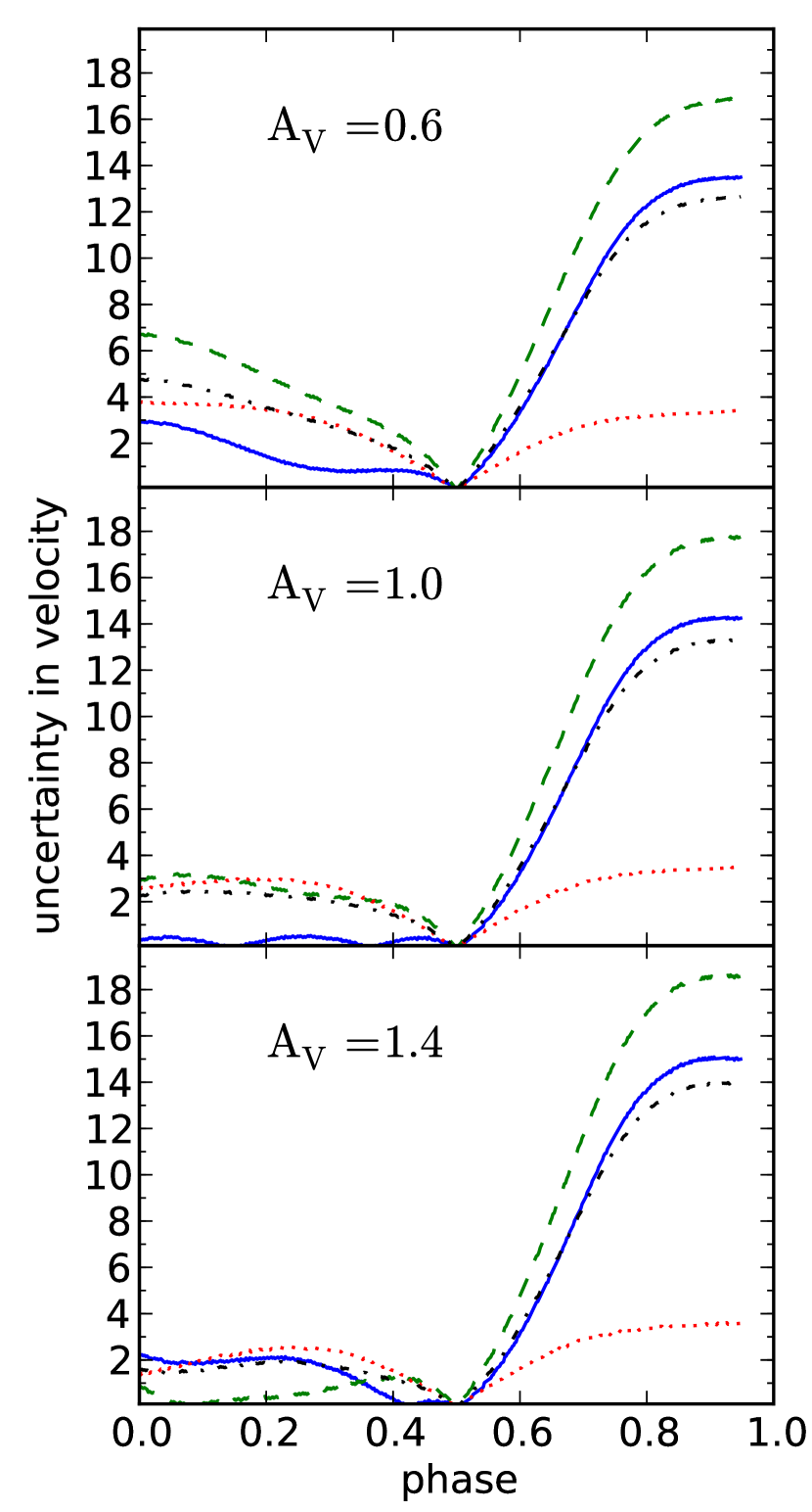
Figure 3: These panels show the uncertainty in velocity (in ${\rm km~{}s}^{-1}$) introduced by using more than one Balmer line in a cross-correlation, for RR Lyrae stars with different $V$-band light curve amplitudes (${\rm A_{V}}$). The solid line shows the uncertainty when the ${\rm H\alpha}$ and ${\rm H\beta}$ lines are used, the dashed line shows the uncertainty when the ${\rm H\alpha}$ and ${\rm H\gamma}$ lines are used, the dot-dashed line shows the uncertainty when ${\rm H\beta}$ and ${\rm H\gamma}$ lines are used, and the dotted line shows the uncertainty when all three lines are used. In general, the uncertainty in velocity introduced by using more than one Balmer line in a cross-correlation is lowest for phases earlier than 0.6 ($\lesssim 4$ ${\rm km~{}s}^{-1}$ for ${\rm A_{V}}=1$ mag), and it decreases with increasing $V$-band amplitude.

To estimate the level of uncertainty introduced by using more than one Balmer line in a cross-correlation, in Figure 3 we show the standard deviation of radial velocities of various Balmer lines as a function of phase for RR Lyrae stars with $V$-band amplitudes ${\rm A_{V}=0.6,1.0,1.4}$ mag. In general, the uncertainty in velocity introduced by using more than one Balmer line in a cross-correlation is lowest for phases earlier than 0.6 ($\lesssim 4$ ${\rm km~{}s}^{-1}$ for ${\rm A_{V}}=1$ mag), and it decreases with increasing $V$-band amplitude.

5 ${\rm A_{g}}$ and ${\rm A_{r}}$ vs. ${\rm A_{V}}$ correlations

Equations 2 to 5 describe the amplitude correlations between radial velocity curves and the $V$-band light curve. To enable use of these equations with RR Lyrae stars that have been observed in the Sloan Digital Sky Survey (SDSS; York et al. 2000) $g$- and $r$-band filters, we also derive the correlations between the light curve amplitudes of RR Lyrae stars observed in SDSS $g$ and $r$ bands and the Johnson $V$ band.

In deriving the correlations, we use the best-fit templates and light curve parameters of 379 $ab$-type RR Lyrae stars observed in SDSS Stripe 82 (see Table 2 in Sesar et al. 2010a). We synthesize each RR Lyrae star’s Johnson $V$-band light curve from the best-fit SDSS $g$- and $r$-band light curves ($g_{LC}(\phi)$ and $r_{LC}(\phi)$) using a photometric transformation given by Equation 10 from Ivezić et al. (2007):

$$V_{LC}(\phi)=g_{LC}(\phi)+0.0688gr_{LC}(\phi)^{3}-0.2056gr_{LC}(\phi)^{2}-0.3838gr_{LC}(\phi)-0.053,$$ (7)

where $gr_{LC}(\phi)=g_{LC}(\phi)-r_{LC}(\phi)$, and $\phi\in[0,1\rangle$ is the phase of pulsation. The $V$-band amplitude is then simply measured from the synthesized light curve.

Having measured $V$-band amplitudes (${\rm A_{V}}$), we can now study how they correlate with SDSS $g$- and $r$-band amplitudes. We find that, within $\sim 0.02$ mag of uncertainty (rms scatter), the $V$-band amplitudes can be calculated as ${\rm 0.9A_{g}}$ and ${\rm 1.21A_{r}}$, where ${\rm A_{g}}$ and ${\rm A_{r}}$ are SDSS $g$- and $r$-band light curve amplitudes of RR Lyrae stars. The 1.21 factor is also obtained for the Johnson $R$ band, by comparing Johnson $V$- and $R$-band light curves of RR Lyrae stars V3, V4, V5, and V10 observed in NGC 5053 by Ferro et al. (2010).

6 Systemic velocity and its uncertainty

In Section 3, the templates were defined to have a zero point at phase of 0.5, since we assumed the radial velocity at phase of 0.5 to be equal to the systemic velocity. Using this definition, the observed radial velocity $v_{obs}$ can be calculated as

$$v_{obs}(\Phi_{obs})=A_{rv}T(\Phi_{obs})+v_{\gamma},$$ (8)

where ${\rm A_{rv}}$ is the amplitude of the radial velocity curve (calculated using Equations 2 to 5), ${\rm T(\Phi_{obs})}$ is the template radial velocity curve, ${\rm\Phi_{obs}}$ is the phase of observation, and ${\rm v_{\gamma}}$ is the systemic velocity.

We use the following equation to model the uncertainty in the systemic velocity (${\rm\sigma_{v_{\gamma}}}$)

$$\sigma_{v_{\gamma}}=(A_{rv}+\sigma_{fit})^{2}[\sigma^{2}_{template}(\Phi_{obs})+(0.1k)^{2}],$$ (9)

where $k$ is the slope of a template between phases 0.4 and 0.6 (1.16, 1.47, 1.54, and 1.42 for the metallic, ${\rm H\alpha}$, ${\rm H\beta}$, and ${\rm H\gamma}$ line templates, respectively). In the above equation, the $\sigma^{2}_{template}(\Phi_{obs})$ term describes the rms scatter in the template at the phase of observation (bottom plots in Figure 1), and the $(0.1k)^{2}$ term describes the error introduced by the uncertainty in phase at which the radial velocity is equal to the systemic (center-of-mass) velocity. These two terms are given in units of velocity amplitude, so they scale with ${\rm A_{rv}}$. To take into account the uncertainty in Equations 2 to 5, we add the rms scatter of the ${\rm A_{rv}}$ vs. ${\rm A_{V}}$ fit to our estimate of the velocity amplitude.

The $(0.1k)^{2}$ term describes our lack of knowledge of the exact phase at which the radial velocity is equal to the systemic (center-of-mass) velocity. In Section 3, we assumed this phase to be at 0.5. However, Oke (1962) used radial velocity measurements of RR Lyrae star SU Dra and found the systemic velocity of this star to be consistent with the observed radial velocity at phase 0.4 (see his Section 6). At this phase, the velocity curves measured from metallic and ${\rm H\gamma}$ lines intersect (i.e., the velocity gradient vanishes, see Figure 3 of Oke 1962). Looking at the radial velocity data for RR Lyrae stars Z Mic and RV Oct shown in Figure 2 of Preston (2011), the metallic and ${\rm H\gamma}$ lines intersect at phases 0.5 and 0.6, respectively. In a different study, Oke (1966) observed the systemic velocity of RR Lyrae star X Ari at phase 0.5. Therefore, we conclude that the uncertainty in the exact phase of systemic velocity is about 0.1. This uncertainty translates into an uncertainty in systemic velocity, which scales with the slope of the template between phases 0.4 and 0.6 ($k$), and naturally, with the amplitude of the velocity curve (${\rm A_{rv}}$). For a typical RR Lyrae star with a $V$-band amplitude of ${\rm A_{V}\sim 1}$ mag, this uncertainty introduces an error of about 13 ${\rm km~{}s}^{-1}$ into the estimate of systemic velocity if the ${\rm H\gamma}$ line is used for radial velocity measurements, or higher if the ${\rm H\beta}$ or ${\rm H\alpha}$ lines are used. This uncertainty is only $\sim 7$ ${\rm km~{}s}^{-1}$ if one uses metallic lines.

7 Discussion and conclusions

We have presented template radial velocity curves of $ab$-type RR Lyrae stars constructed from high-precision measurements of ${\rm H\alpha}$, ${\rm H\beta}$, and ${\rm H\gamma}$ lines. Compared to the template radial velocity curve (solid line in the top right plot of Figure 1), the shape of observed ${\rm H\alpha}$ velocity curves varies the most (up to $\sim 10$ ${\rm km~{}s}^{-1}$). The observed metallic lines curves show the least amount of variability ($\sim 3\%$ of ${\rm A_{rv}}$ or $\sim 2$ ${\rm km~{}s}^{-1}$ for a RR Lyrae star with ${\rm A_{V}}=1.0$ mag), followed by ${\rm H\gamma}$ and ${\rm H\beta}$ velocity curves ($\sim 3\%$ to $4\%$ of ${\rm A_{rv}}$ or $\sim 4$ ${\rm km~{}s}^{-1}$). The fluctuation in the shape of metallic, ${\rm H\gamma}$ and ${\rm H\beta}$ velocity curves is consistent with measurement errors, and implies little or no variation in the shape of velocity curves over a wide range of $V$-band amplitudes (0.6 to 1.1 mag), even for RR Lyrae stars that are undergoing Blazkho modulations.

We have found tight correlations (rms scatter $<3.4$ ${\rm km~{}s}^{-1}$) between amplitudes of Balmer lines velocity curves (${\rm A_{rv}}$) and $V$-band light curves (${\rm A_{V}}$). A similar correlation, but for metallic lines, was first reported by L91. We also find that the ratio of amplitudes of Balmer versus metallic lines velocity curves decreases towards shorter wavelengths, and is 1.90, 1.54, and 1.39 for ${\rm H\alpha}$, ${\rm H\beta}$, and ${\rm H\gamma}$ lines. This pattern basically follows the depth of formation of lines; the ${\rm H\gamma}$ line forms closer to the photosphere than the ${\rm H\alpha}$ line, and therefore has smaller variations in the radial velocity.

The correlations derived in this paper have the potential to significantly improve the precision of systemic velocities of RR Lyrae stars estimated from a small number of radial velocity measurements of Balmer lines. For example, Equation 5 indicates that previous studies that used the ${\rm H\gamma}$ velocity curve of X Ari (${\rm A_{rv}\sim 85}$ ${\rm km~{}s}^{-1}$, ${\rm A_{V}\sim 1.0}$ mag) may have introduced up to $\sim 15$ ${\rm km~{}s}^{-1}$ of uncertainty in their estimates of systemic velocities for RR Lyrae stars with $V$-band amplitudes of 0.6 or 1.3 mag. Such uncertainties can be now be eliminated by using Balmer line radial velocity templates and Equations 3 to 5 presented in this work.

We find the dominant source of uncertainty in the systemic velocity to be the phase at which the radial velocity is equal to the systemic velocity. We have estimated this uncertainty in phase to be about 0.1. For a RR Lyrae star with a $V$-band amplitude of ${\rm A_{V}=1.0}$ mag, this uncertainty in phase translates into a velocity uncertainty of about 13 ${\rm km~{}s}^{-1}$. A repeat of the analysis by Oke (1962) (see his his Section 6) on radial velocity data used in our work may provide more insight into this fundamental uncertainty.

Regrettably, we could not obtain radial velocity measurements of the ${\rm H\delta}$ line (due to low signal-to-noise ratio in echelle data; George W. Preston, private communication), and were thus unable to construct a template curve or establish a correlation between the ${\rm H\delta}$ velocity amplitude and the $V$-band light curve amplitude. This is quite unfortunate as this line is often used in radial velocity measurements of RR Lyrae stars and is usually accessible (along with ${\rm H\beta}$ and ${\rm H\gamma}$ lines) to most low-resolution spectrographs, such as DBSP (Oke & Gunn, 1982) or LRIS (Oke et al., 1995). A spectroscopic survey that would provide velocity measurements of the ${\rm H\delta}$ line for several RR Lyrae stars would be very useful, and would allow the extension of this work to the ${\rm H\delta}$ line.

By deriving correlations between light curve amplitudes of RR Lyrae stars observed in SDSS $g$ and $r$ bands and the Johnson $V$ band (Section 5), we have expanded the applicability of Equations 3 to 5 to a large number of already or soon to be observed RR Lyrae stars. For example, there are $\sim 380$ $ab$-type RR Lyrae stars with measured light curve parameters (period, epoch of maximum light, amplitudes in SDSS $ugriz$ band, etc.) that have been observed in SDSS stripe 82 (Sesar et al., 2010a), a large fraction of which have spectroscopic observations (de Lee, 2008). While the systemic velocities of these stars have already been measured (de Lee, 2008), these measurements could be improved using Equations 3 to 5, leading to better estimates of kinematic properties of the Galactic halo.

Then there are multi-epoch, wide-area surveys such as the Lincoln Near-Earth Asteroid Research (LINEAR; Sesar et al. 2011) and Palomar Transient Factory (PTF; Law et al. 2009), which are currently finding thousands of RR Lyrae stars within 30 kpc from the Sun (Sesar, 2011). Some of these stars have previously been spectroscopically observed by SDSS, and many more are expected to be observed by the upcoming low-resolution spectroscopic survey LEGUE ($R=1800$; Deng et al. 2012). By using light curve parameters of RR Lyrae stars from LINEAR and PTF, radial velocities from LEGUE, and Equations 3 to 5, one could easily construct a sample of RR Lyrae stars with precise positions and 3D kinematics, and use them to search for halo substructures within 30 kpc from the Sun.

And finally, the Large Synoptic Survey Telescope (LSST; Ivezić et al. 2008) is expected to be able to observe RR Lyrae stars as far as 360 kpc from the Sun (Oluseyi et al., 2012). With RR Lyrae stars detected at these distances, LSST will be able to search for halo streams and dwarf satellite galaxies within a significant fraction of the Local Group. Due to faintness of these distant RR Lyrae stars ($V\lesssim 23.4$), the spectroscopic followup will most likely involve observations of Balmer lines at low resolutions ($R\sim 1500$), making the tools presented in this work a natural choice for the measurement of their systemic velocities.

Table 1: ASAS RR Lyrae Stars

Star	R.A.(J2000)	Dec(J2000)	${\rm A_{V}}^{a}$	${\rm V_{max}}^{b}$	Blazhkoc	$N_{obs}$	Metallic ${\rm A_{rv}}^{d}$	${\rm H\alpha}$ ${\rm A_{rv}}^{d}$	${\rm H\beta}$ ${\rm A_{rv}}^{d}$	${\rm H\gamma}$ ${\rm A_{rv}}^{d}$
	(hr $\arcmin$ $\arcsec$)	($\arcdeg$ $\arcmin$ $\arcsec$)	(mag)	(mag)			(${\rm km~{}s}^{-1}$)	(${\rm km~{}s}^{-1}$)	(${\rm km~{}s}^{-1}$)	(${\rm km~{}s}^{-1}$)
Z Mic	21 16 22.71	-30 17 03.1	0.64	11.32	Yes	166	51.6	101.7	79.5	70.3
CD Vel	09 44 38.24	-45 52 37.2	0.87	11.66	Yes	193	53.5	105.7	82.7	73.7
WY Ant	10 16 04.95	-29 43 42.4	0.95	10.37	No	130	62.2	117.8	93.3	83.1
DT Hya	11 54 00.18	-31 15 40.0	0.98	12.53	No	96	62.3	109.9	93.2	83.1
XZ Aps	14 52 05.43	-79 40 46.6	1.10	11.94	No	241	62.1	118.4	100.2	92.0
RV Oct	13 46 31.75	-84 24 06.4	1.13	10.53	Yes	193	63.1	117.8	96.5	90.1

Figure 2: Correlations between radial velocity amplitude, $A_{rv}$, and $V$-band light curve amplitude, $A_{V}$, for radial velocities measured from metallic lines (top left panel), ${\rm H\alpha}$ line (top right panel), ${\rm H\beta}$ line (bottom left panel), and ${\rm H\gamma}$ line (bottom right panel). The solid lines show an unweighted linear least-squares fit to plotted points (Equations 2 to 5), and ${\rm\sigma_{rms}}$ indicates the rms scatter of the fit in ${\rm km~{}s}^{-1}$. The dashed line in the top left panel shows the fit obtained by L91 (see Section 4 for more details). Even though Liu’s sample spans a much greater range of $V$-band amplitudes than ours and has more stars, the two fits agree within uncertainties (rms scatter of $\sim 2.5$ ${\rm km~{}s}^{-1}$), indicating the our fit’s robustness.

References

- Blazhko (1907) Blazhko, S. 1907, Astron. Nachr., 175, 325
- Carlin et al. (2012) Carlin, J. L., Yam, W., Casetti-Dinescu, D., et al. 2012, accepted to ApJ (also arXiv:1205.2371)
- Casetti-Dinescu et al. (2009) Casetti-Dinescu, D. I., Girard, T. M., Majewski, S. R., et al. 2009, ApJ, 701, 29
- de Lee (2008) de Lee, N. 2008, Ph.D. dissertation, Michigan State University, Michigan
- Deng et al. (2012) Deng, L. Newberg, H. J., Liu, C., Carlin, J. L., et al. 2012, submitted to RAA (also arXiv:1206.3578)
- Duffau et al. (2006) Duffau, S., Zinn, R., Vivas, A. K., Carraro, G., Méndez, R. A., Winnick, R., & Gallart, C. 2006, ApJ, 636, L97
- Ferro et al. (2010) Ferro, A. A., Giridhar, S., & Bramich, D. M. 2010, MNRAS, 402, 226
- For et al. (2011) For, B.-Q., Preston, G. W., & Sneden, C., 2011, ApJS, 194, 38
- Hawley & Barnes (1985) Hawley, S. L. & Barnes, T. G., III 1985, PASP, 97, 551
- Ivezić et al. (2007) Ivezić, Ž., Smith, J. A., Miknaitis, G., et al. 2007, AJ, 134, 973
- Ivezić et al. (2008) Ivezić, Ž., Tyson, J. A., Acosta, E., et al. 2008, arXiv:0805.2366
- Johnston et al. (2012) Johnston, K. V., Sheffield, A. A., Majewski, S. R., & Sharma, S. 2012, arXiv:1202.5311
- Keller et al. (2008) Keller, S. C., Murphy, S., Prior, S. et al. 2008, ApJ, 678, 851
- Kollmeier et al. (2009) Kollmeier, J. A., Gould, A., Shectman, S., et al. 2009, ApJ, 705, L158
- Kovács (2003) Kovács, G. 2003, MNRAS, 342, 58
- Law et al. (2009) Law, N. M., Kulkarni, S. R., Dekany, R. G., et al. 2009, PASP, 121, 1395
- Layden (1994) Layden, A. C. 1994, AJ, 108, 1016
- Liu (1991) Liu, T. 1991, PASP, 103, 205 (L91)
- Miceli et al. (2008) Miceli, A., Rest, A., Stubbs, C. W., et al. 2008, ApJ, 678, 865
- Oke (1962) Oke, J. B. 1962, ApJ, 136, 393
- Oke (1966) Oke, J. B. 1966, ApJ, 145, 468
- Oke et al. (1995) Oke, J. B., Cohen, J. G., Carr, M., et al. 1995, PASP, 107, 375
- Oke & Gunn (1982) Oke, J. B. & Gunn, J. E. 1982, PASP, 94, 586
- Oluseyi et al. (2012) Oluseyi, H. M., Becker, A. C., Culliton, et al. 2012, AJ, 144, 9
- Pojmański (1997) Pojmański G., 1997, Acta Astron., 47, 467
- Preston (2011) Preston, G. W. 2011, AJ, 141, 6
- Prior et al. (2009) Prior, S. L., Da Costa, G. S., Keller, S. C., & Murphy, S. J. 2009, ApJ, 691, 306
- Sesar et al. (2007) Sesar, B., Ivezić, Ž., Lupton, R. H., et al. 2007, AJ, 134, 2236
- Sesar et al. (2010a) Sesar, B., Ivezić, Ž., Grammer, S. H., et al. 2010a, ApJ, 708, 717
- Sesar et al. (2010b) Sesar, B., Vivas, A. K., Duffau, S. & Ivezić, Ž. 2010b, ApJ, 717, 133
- Sesar (2011) Sesar, B. 2011, “RR Lyrae Stars, Metal-Poor Stars, and the Galaxy”, Carnegie Observatories Astrophysics Series Vol.5, p. 135, ed. Andrew McWilliam, Pasadena, CA
- Sesar et al. (2011) Sesar, B., Stuart, J. S., Ivezić, Ž., et al. 2011, AJ, 142, 190
- Sesar et al. (2012) Sesar, B., Cohen, J. G., Levitan, D., et al. 2012, accepted to ApJ (also arXiv:1206.0269)
- Smith (1995) Smith, H. A., 1995, RR Lyrae Stars (Cambridge University Press)
- Szczygiel & Fabrycky (2007) Szczygiel, D. M. & Fabrycky, D. C. 2007, MNRAS, 377, 1263
- Vivas et al. (2001) Vivas, A. K., Zinn, R., Andrews, P., et al. 2001, ApJ, 554, 33
- Vivas et al. (2005) Vivas, A. K., Zinn, R., & Gallart, C. 2005, AJ, 129, 189
- Watkins et al. (2009) Watkins, L. L., Evans, N. W., Belokurov, V., et al. 2009, MNRAS, 398, 1757
- York et al. (2000) York, D. G., Adelman, J., Anderson, J. E., et al. 2000, AJ, 120, 1579