A Gravitational Redshift Determination of the Mean Mass of White Dwarfs. DBA and DB Stars

Abstract

We measure apparent velocities ($v_{\rm app}$) of absorption lines for 36 white dwarfs (WDs) with helium-dominated atmospheres – 16 DBAs and 20 DBs – using optical spectra taken for the European Southern Observatory SN Ia progenitor survey (SPY). We find a difference of $6.9\pm 6.9$ km s^-1 in the average apparent velocity of the H$\alpha$ lines versus that of the He I 5876 Å for our DBAs. This is a measure of the blueshift of this He line due to pressure effects. By using this as a correction, we extend the gravitational redshift method employed by Falcon et al. (2010) to use the apparent velocity of the He I 5876 Å line and conduct the first gravitational redshift investigation of a group of WDs without visible hydrogen lines. We use biweight estimators to find an average apparent velocity, $\langle v_{\rm app}\rangle_{\rm BI}$, (and hence average gravitational redshift, $\langle v_{\rm g}\rangle_{\rm BI}$) for our WDs; from that we derive an average mass, $\langle M\rangle_{\rm BI}$. For the DBAs, we find $\langle v_{\rm app}\rangle_{\rm BI}=40.8\pm 4.7$ km s^-1 and derive $\langle M\rangle_{\rm BI}=0.71^{+0.04}_{-0.05}\,M_{\odot}$. Though different from $\langle v_{\rm app}\rangle$ of DAs (32.57 km s^-1) at the 91% confidence level and suggestive of a larger DBA mean mass than that for normal DAs derived using the same method ($0.647^{+0.013}_{-0.014}\,M_{\odot}$; Falcon et al., 2010), we do not claim this as a stringent detection. Rather, we emphasize that the difference between $\langle v_{\rm app}\rangle_{\rm BI}$ of the DBAs and $\langle v_{\rm app}\rangle$ of normal DAs is no larger than 9.2 km s^-1, at the 95% confidence level; this corresponds to roughly $0.10\,M_{\odot}$. For the DBs, we find $\langle v_{\rm app}^{\rm He}\rangle_{\rm BI}=42.9\pm 8.49$ km s^-1 after applying the blueshift correction and determine $\langle M\rangle_{\rm BI}=0.74^{+0.08}_{-0.09}\,M_{\odot}$. The difference between $\langle v_{\rm app}^{\rm He}\rangle_{\rm BI}$ of the DBs and $\langle v_{\rm app}\rangle$ of DAs is $\leq 11.5$ km s^-1 ($\sim 0.12\,M_{\odot}$), at the 95% confidence level. The gravitational redshift method indicates much larger mean masses than the spectroscopic determinations of the same sample by Voss et al. (2007). Given the small sample sizes, it is possible that systematic uncertainties are skewing our results due to the potential of kinematic substructures that may not average out. We estimate this to be unlikely, but a larger sample size is necessary to rule out these systematics.

1. Introduction

In Falcon et al. (2010), we show that the gravitational redshift method is an effective tool for measuring mean masses of groups of white dwarfs (WDs) and has the advantage of being mostly independent from the spectroscopic method (e.g., Bergeron et al., 1992). Falcon et al. (2010) investigate normal DAs, the largest class of WDs. The next logical step is to ask whether the method can be applied to the second largest class, DBs, which constitute 20% of all WDs below $T_{\rm eff}\sim 17,000$ K  and $\sim 9$% of WDs at higher temperatures (Beauchamp et al., 1996; Bergeron et al., 2011).

However, the gravitational redshift method historically uses the apparent velocities of hydrogen Balmer line cores. The work by Shipman & Mehan (1976) and by Grabowski et al. (1987) show H$\alpha$ to be suitable for this purpose since it are not significantly affected by pressure shifts. Pure DB spectra exhibit only helium lines, and as Greenstein & Trimble (1967) first pointed out, using WD photospheric helium lines for gravitational redshift measurements can be difficult due to the likelihood of systematics introduced by pressure effects. These systematics include that, in theory, and with some experimental support (e.g., Berg et al., 1962; Pérez et al., 2003), different helium lines can be pressure shifted by different amounts, in different (blue or red) directions, and with a dependency on temperature (e.g., Griem et al., 1962; Bassalo & Cattani, 1976; Dimitrijevic & Sahal-Brechot, 1990; Omar et al., 2006). For this reason, attempts at gravitational redshift measurements for helium-dominated WDs have been sparse.

Koester (1987) measures line shifts of He I 4026, 4471, 4713, and 4922 Å in the spectrum of the common proper motion star WD 0615-591 and of He I 4471 and 4922 Å in the wide binary WD 2129+000. These line shifts are negative (blue), meaning that the magnitude of the pressure effects are larger than the magnitude of the gravitational redshift, which, in this case, are opposing each other. The fact that these WDs are relatively cool (Bergeron et al., 2011) is consistent with the expectation that pressure effects should be significant; we will elaborate on this point in Section 3.6. Koester (1987) concludes that due to the state of the theory at the time – laboratory measurements and theoretical predictions often disagreed on the magnitude and sometimes even sign of the shift – he cannot deduce meaningful gravitational redshifts for these two DBs.

Wegner et al. (1989) measure the gravitational redshift for the Hyades DBA WD 0437+138 using H$\alpha$ and mention that the velocity “…is unaffected by the pressure shift problems of helium” while providing no further detail. The importance of van der Waals broadening in cool helium-dominated atmospheres (Bergeron et al., 1991), however, was perhaps not yet well-established. In hindsight, it is likely that H$\alpha$ in this WD is significantly affected.

The sample of common proper motion binary and cluster WDs in Reid (1996) contains three targets with helium-dominated atmospheres. For both DBAs, WD 0437+138 and WD 1425+540, Reid determines different gravitational redshifts from using H$\alpha$ than from H$\beta$. He mentions that this discrepancy could be because of pressure shifts due to the high atmospheric helium abundance and deems the H$\alpha$ result as the better redshift estimate since this line should be less affected than H$\beta$. Reid also measures, like Koester (1987), negative shifts of helium lines for the DB WD 2129+000. One of his measured lines (He I 4921, 5015, and 6678 Å) is in common with that of Koester (1987).

With more recent high-resolution spectroscopic observations of helium-atmosphere WDs (Voss et al., 2007) and with the method of Falcon et al. (2010), we now have the tools to revisit the gravitational redshift of DBs. Such an investigation is a valuable check to the latest spectroscopic work (Bergeron et al., 2011), the analysis of which is nontrivial due in part to the challenge of interpreting pressure-broadened helium lines (Beauchamp et al., 1997; Beauchamp & Wesemael, 1998; Beauchamp et al., 1999).

In Section 3.6 we discuss using the apparent velocity of the He I 5876 Å line in the context of our work and, as Wegner & Reid (1987) suggest, check for consistency within the DBA sample of the apparent velocities of both the hydrogen and helium line species. In Section 4.1 we perform the original gravitational redshift method that uses hydrogen Balmer lines on the DBAs, which results in the most direct comparison with the DAs from Falcon et al. (2010). Then in Section 4.2 we extend the method to WDs with only helium lines.

2. Observations

We use spectroscopic data from the European Southern Observatory (ESO) SN Ia progenitor survey (SPY; Napiwotzki et al., 2001). These observations, taken using the UV-Visual Echelle Spectrograph (UVES; Dekker et al., 2000) at Kueyen, Unit Telescope 2 of the ESO VLT array, constitute the largest, homogeneous, high-resolution (0.36 Å or $\sim 16$ km s^-1 at H$\alpha$) spectroscopic dataset for WDs. We obtain the pipeline-reduced data online through the publicly available ESO Science Archive Facility.

2.1. Samples

The helium-atmosphere WDs in our sample are derived from the SPY objects analyzed by Voss et al. (2007). Out of their 38 DBAs with atmospheric parameter determinations, we exclude one magnetic WD, one DO, and twelve cool WDs with $T_{\rm eff}\lesssim$16,500 K. For these twelve, Voss et al. (2007) fix the surface gravity at log $g$=8 in order to obtain spectral fits; this forfeits our ability to properly compare these stars with our gravitational redshift results. Due to data quality, we are unable to satisfactorily measure apparent velocities ($v_{\rm app}$) of H$\alpha$ for an additional eight, which leaves us with 16 DBAs. Keep in mind that for these objects, the atmospheric abundance of hydrogen is small and H$\alpha$ is often barely visible.

Out of the 31 measured DBs from Voss et al. (2007), we exclude nine cool WDs and two known to have cool companions (Zuckerman & Becklin, 1992; Farihi et al., 2005; Hoard et al., 2007). We end up with 20 normal DBs and 36 helium-atmosphere WDs overall.

Four of our DBAs show Ca II lines in their spectra, giving them the additional classification as DBAZ (Koester et al., 2005b; Voss et al., 2007), and two DBs are classified as DBZs (Voss et al., 2007). Since the SPY Collaboration has not reported any of our WDs to have stellar companions, we presume them to not be in close binary systems, though two of our DBAs (WD 0948+013, WD 2154-437) and two of our DBs (WD 0615-591, WD 0845-188) are in common proper motion or wide binary systems (Luyten, 1949; Wegner, 1973; Caballero, 2009). The lack of detectable Zeeman splitting implies that our targets also do not harbor significant ($\gtrsim$100 kG) magnetic fields (e.g., Koester et al., 2009).

The WDs in our sample have not been classified in the literature as potential members of the thick disk or halo stellar populations. We therefore make the assumption that all of these WDs belong to the thin disk – a necessary assumption for our analysis (see Section 3.3). Nearly all ($>$90%) of the SPY WDs that have been studied kinematically are classified as thin disk objects (Pauli et al., 2006; Richter et al., 2007).

3. Using Gravitational Redshift to Determine a Mean Mass

We use the methods described in Falcon et al. (2010). To summarize, we measure the apparent velocity of the H$\alpha$ line for an ensemble of WDs. We correct these velocities so that the WDs are in a comoving reference frame. The average apparent velocity then becomes the average gravitational redshift because random stellar radial velocities average out. By using the mass-radius relation from WD evolutionary models, we translate this average gravitational redshift to an average mass.

In this work, we add two extensions to the method: (1) a different estimator of central location of the distribution better suited for small sample sizes (Section 3.5) and (2) use of the He I 5876 Å line for helium-atmosphere WDs (Section 3.6).

3.1. Gravitational Redshift

In the weak-field limit, the general relativistic effect of gravitational redshift can be observed as a velocity shift in absorption lines and is expressed as

$$v_{g}=\frac{c\Delta\lambda}{\lambda}=\frac{GM}{Rc}$$ (1)

where $G$ is the gravitational constant, and $c$ is the speed of light. In our case, $M$ is the WD mass, and $R$ is the WD radius.

The apparent velocity of an absorption line is the sum of this gravitational redshift and the stellar radial velocity: $v_{\rm app}=v_{\rm g}+v_{\rm r}$. These two components cannot be explicitly separated for individual WDs without an independent $v_{\rm r}$ measurement or mass determination. We break this degeneracy for a group of WDs by assuming that the sample is comoving and local. After we correct each $v_{\rm app}$ to the local standard of rest (LSR), only random stellar motions dominate the dynamics of our sample. These average out, and the mean apparent velocity becomes the mean gravitational redshift: $\langle v_{\rm app}\rangle=\langle v_{\rm g}\rangle$.

3.2. Velocity Measurements

Collisional (Stark) broadening effects cause asymmetry in the wings of absorption lines for the hydrogen Balmer series, making it difficult to measure a velocity centroid (Shipman & Mehan, 1976; Grabowski et al., 1987). However, these effects are not significant in the sharp, non-LTE H$\alpha$ and H$\beta$ Balmer line cores. We use both of these line cores in Falcon et al. (2010). In the SPY spectra of DBAs, though, we do not observe the non-LTE line cores, but the H$\alpha$ line centers are still distinct. For H$\alpha$ the pressure shift should remain very small ($<1$ km s^-1) within a few Å of the line center (Grabowski et al., 1987).

Reid (1996) measures the gravitational redshift of the DBA WD 0437+138 using the line center since he observes no sharp line core. While cautioning that pressure effects may be significant, he determines a high mass of $0.748\pm 0.037\,M_{\odot}$. Bergeron et al. (2011) determine a spectroscopic mass of $0.74\pm 0.06\,M_{\odot}$ for this WD. For at least this one case, then, gravitational redshifts of the line center give a result consistent with the spectroscopic method.

Van der Waals broadening due to neutral helium may also signficantly affect line shapes below $T_{\rm eff}=$16,500 K (Koester et al., 2005a; Voss et al., 2007). We avoid this systematic by not including targets in that range of $T_{\rm eff}$.

We measure $v_{\rm app}$ for each DBA in our sample by fitting a Gaussian profile to the H$\alpha$ line center using GAUSSFIT, a non-linear least-squares fitting routine in IDL. If multiple epochs of observation exist, we combine the measurements as a mean weighted according to the uncertainties returned by the fitting routine. Eight out of our 16 DBAs have two epochs of observation. Table 1 lists these measurements for the DBA sample including those for each epoch of observation and the final adopted values.

By inspecting the $v_{\rm app}$ measurements between epochs, we notice they differ by more than a typical measurement uncertainty; the mean difference between epochs of the same target is 9.20 km s^-1 while the mean measurement uncertainty for all observations is 3.05 km s^-1. Since we presume none of our targets to be in close binary systems (Section 2.1), reflex orbital motion cannot be the culprit, and therefore it is evident that we are underestimating our individual measurement uncertainties. To more accurately represent our adopted $\delta v_{\rm app}$ values for each target, we multiply all observation $\delta v_{\rm app}$ values by the factor we find above: the ratio of the mean difference in apparent velocity between epochs and the mean apparent velocity measurement uncertainty. For the DBA sample, this factor is 3.02. The final adopted values for $\delta v_{\rm app}$ listed in Column 3 in Table 1 include this adjustment, and the observation values in Column 8 are the values before the adjustment.

For the DBAs and the DBs, we also measure $v_{\rm app}$ using the He I 5876 Å line and list the results in Tables 2 and 3, respectively. Here, too, we apply a multiplicative factor to all observation $\delta v_{\rm app}$ values to better represent our measurement uncertainties. These factors are 2.12 and 2.49 for the two samples. The methodology for line center fitting is the same as used for the H$\alpha$ Balmer line.

3.3. Comoving Approximation

We measure a mean gravitational redshift by assuming that our WDs are a comoving, local sample. With this assumption, only random stellar motions dominate the dynamics of our targets; this falls out when we average over the sample.

For this assumption to be valid, at least as an approximation, our WDs must belong to the same kinematic population; in our work, this is the thin disk. We achieve a comoving group by correcting each measured $v_{\rm app}$ to the kinematical LSR described by Standard Solar Motion (Kerr & Lynden-Bell, 1986). Column 4 in Tables 1 - 3 lists the LSR corrections applied to each target. In Falcon et al. (2010), we show in detail that this is a suitable choice of reference frame for a sample consisting of thin disk WDs.

If the targets in our sample belong predominantly to the thick disk, for example, our chosen reference frame will fail to produce a group of objects that is at rest with respect to the LSR, introducing a directional bias into our measured $\langle v_{\rm app}\rangle$. This is because the thick disk population lags behind the thin disk as it rotates about the Galactic center ($\sim 40$ km s^-1; Gilmore et al., 1989).

In contrast to the work on DAs in Falcon et al. (2010), we lack the sample size to empirically demonstrate whether or not our WDs move with the LSR. Therefore, as we state in Section 2.1, we must assume our targets are thin disk objects.

Our WDs must also reside at distances that are small compared to the size of the Galaxy so that systematics introduced by the Galactic kinematic structure are not significant. Nine of our DBAs and twelve of our DBs have published distance determinations in the range of $\sim 25$ to $\sim 260$ pc (Routly, 1972; Wegner, 1973; Koester et al., 1981; Farihi et al., 2005; Castanheira et al., 2006; Limoges & Bergeron, 2010; Bergeron et al., 2011). We assume the others are at distances comparable to the rest of the SPY sample which Pauli et al. (2006) determine spectroscopically to be mostly ($\gtrsim$90 %) within 200 pc with a mean of $\sim$100 pc. Over these distances, the velocity dispersion with varying scale height above the disk remains modest (Kuijken & Gilmore, 1989), and differential Galactic rotation is negligible (Fich et al., 1989).

3.4. Deriving a Mean Mass

To translate the mean apparent velocity $\langle v_{\rm app}\rangle$ to a mean mass, we invoke two constraints: (1) we need the mass-radius relation from an evolutionary model, and (2) since the WD radius does slightly contract during its cooling sequence, we need an estimate of the position along this track for the average WD in our sample (i.e., a mean $T_{\rm eff}$).

Our evolutionary models use $M_{\rm He}/M_{\star}=10^{-2}$ for the helium surface-layer mass, and, since we are interested in WDs with helium-dominated atmospheres, we use $M_{\rm H}/M_{\star}=0$ for the hydrogen surface-layer mass. See Montgomery et al. (1999) for a more complete description of our models. Our dependency on evolutionary models is small. We are interested in the mass-radius relation from these models, and this is relatively straight-forward since WDs are mainly supported by electron degeneracy pressure, making the WD radius a weak function of temperature. We estimate that varying the C/O ratio in the core affects the radius by less than 0.7%.

3.5. Appyling the Method to Small Samples

Besides atmospheric composition, the difference between the WD sample in Falcon et al. (2010) and the ones in this paper is sample size; the DA sample boasts 449 targets while our DBA and DB samples contain 16 and 20, respectively. For large numbers such as for the DAs, the (arithmetic) mean is the preferred estimator of central location of the distribution. For small numbers, however, this is not necessarily so.

In lieu of the mean, we use the biweight central location estimator and the biweight scale estimator as recommended by Beers et al. (1990) for a kinematic sample of our size. For a discussion on the biweight and its statistical properties of resistance, robustness, and efficiency as they relate to sample size and type of distribution, see Beers et al. (1990).

The biweight central location estimator is defined as

$$C_{\rm BI}=M+\frac{\sum_{|u_{i}|<1}(x_{i}-M)(1-u_{i}^{2})^{2}}{\sum_{|u_{i}|<1}(1-u_{i}^{2})^{2}},$$ (2)

where $x_{i}$ are the data, $M$ is the sample median, and $u_{i}$ are given by

$$u_{i}=\frac{(x_{i}-M)}{c\,{\rm MAD}}.$$ (3)

We set the “tuning constant” $c=7.0$ (a slight increase from the recommended $c=6.0$ listed in Beers et al. (1990)) so that no data rejection occurs. Notice that $C_{\rm BI}$ approaches the arithmetic mean in the limit where $c\rightarrow\infty$. MAD (median absolute deviation from the sample median) is defined as

$${\rm MAD}={\rm median}(|x_{i}-M|).$$ (4)

We calculate $C_{\rm BI}$ iteratively, taking $M$ as a first guess, substituting the calculated $C_{\rm BI}$ as the improved guess, and continuing to convergence.

The biweight scale estimator is defined as

$$S_{\rm BI}=n^{1/2}\frac{\left[\sum_{|u_{i}|<1}(x_{i}-M)^{2}(1-u_{i}^{2})^{4}\right]^{1/2}}{\left|\sum_{|u_{i}|<1}(1-u_{i}^{2})(1-5u_{i}^{2})\right|}.$$ (5)

Here we set $c=9.0$ (within the expression for $u_{i}$) as recommended by Beers et al. (1990).

To determine the uncertainty of the biweight, we use a Monte Carlo approach. We adopt the standard deviation of biweight values from 30,000 simulated $v_{\rm app}$ distributions. Each simulated distribution randomly samples from a convolution of two Gaussians. One represents the measured $v_{\rm app}$ distribution by using the biweight scale estimator $S_{\rm BI}$ (analogous to standard deviation) of the sample as the width of the Gaussian. The other accounts for the individual apparent velocity measurement uncertainties by drawing from a Gaussian with a width equal to each $\delta v_{\rm app}$ from the sample.

From here on we use the subscript BI to denote the biweight central location estimator, $C_{\rm BI}$, and biweight scale estimator, $S_{\rm BI}$, as used in lieu of the arithmetic mean and standard deviation, respectively.

3.6. Pressure Shifts of Helium Lines

As described in Section 1, helium line centroids are expected to shift due to pressure effects, and the magnitude and direction of the shift is thought to depend on the specific line. For that reason, we focus on measurements of a single helium line, He I 5876 Å. Theoretical calculations give a negative (blue) Stark shift of the He I 5876 Å line for electron densities corresponding to WD photospheres and in the temperature range relevant to our investigation (e.g., Griem et al., 1962; Dimitrijevic & Sahal-Brechot, 1990); the experiment by Heading et al. (1992) confirms the sign of the shift.

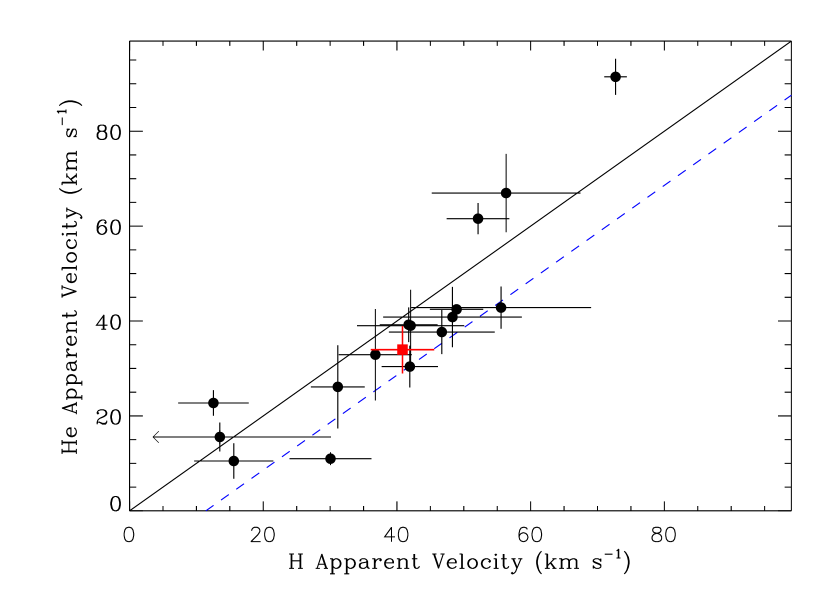
Figure 1.— Plot of apparent velocity $v_{\rm app}$ obtained from H$\alpha$ versus $v_{\rm app}$ obtained from the He I 5876 Å line for the targets in our DBA sample. The intersection of $\langle v_{\rm app}\rangle_{\rm BI}$ and $\langle v_{\rm app}^{\rm He}\rangle_{\rm BI}$ (filled, red square) lies below the unity line; the two average values differ by $6.9\pm 6.9$ km s^-1. The dashed, blue line represents a theoretical blueshift of the He I line derived from Dimitrijevic & Sahal-Brechot (1990) for $T=16,500$ K and $n_{\rm e}=10^{17}$ cm^-3 (see Section 3.6).

We search for this expected blueshift using our sample of DBAs, whose spectra show both the He I 5876 Å line and the H$\alpha$ Balmer line center that should not be affected by pressure shifts. Figure 1 shows a comparison of apparent velocities measured from these lines, and indeed the intersection (filled, red square) of the average (biweight) values lies below the unity line.

Using the calculated shifts from Dimitrijevic & Sahal-Brechot (1990), we plot a dashed line in Figure 1 indicating the deviation from unity for plasma conditions corresponding to temperature $T=16,500$ K and electron density $n_{\rm e}=10^{17}$ cm^-3. This should represent an overestimate of the expected shift based on theory. $T_{\rm eff}=16,500$ K is the lower limit for the WDs in our sample, and not only does the magnitude of the shift increase with decreasing temperature, but it tracks exponentially so that the effect is more exaggerated at lower $T$. Furthermore, although $n_{\rm e}=10^{17}$ cm^-3 is typical for WD photospheres, we are concerned with absorption line centers. These are formed higher in the atmosphere where the density is lower and the shift should be less. As expected, the intersection of our measured biweight values lies between the unity line and the blueshift overestimate.

The presence of hydrogen in a helium-dominated atmosphere may also affect the atmospheric pressure and therefore electron density because of its relatively high opacity; in our temperature range, the opacity of hydrogen can be an order of magnitude greater than that of helium. From Voss et al. (2007), the mean atmospheric hydrogen abundance for the WDs in our DBA sample is H/He= $10^{-3.29}$ with the highest abundance of any WD being H/He= $10^{-2}$. At these abundances, this opacity effect should be negligible, and the dependency of the distribution of pressure shifts on electron density should only be due to the intrinsic mass distribution.

The average apparent velocity of the DBAs in Figure 1 as measured from H$\alpha$ is $\langle v_{\rm app}\rangle_{\rm BI}=40.8\pm 4.7$ km s^-1; the average velocity as measured from the He I 5876 Å line is $\langle v_{\rm app}^{\rm He}\rangle_{\rm BI}=34.0\pm 5.0$ km s^-1. The measured difference of $6.9\pm 6.9$ km s^-1 is blueshifted and exactly at the 1-sigma boundary of our measurement precision.

With assumptions this measured blueshift can be used as a correction to apply to the average apparent velocity of DB WD samples in order to estimate an average gravitational redshift. First, one must assume that DBAs are not fundamentally different from DBs in a way that would manifest as different mean masses. Voss et al. (2007) detect various amounts of hydrogen in most (55%) of the helium-dominated WDs in their sample and find similar spectroscopic mass distributions between the DBAs and DBs. Bergeron et al. (2011) also find no significant differences between the masses of the two groups. This provides evidence to the idea of Weidemann & Koester (1991) that the DBA subclass is not distinct from its parent class but rather the observationally detectable end of a continuous distribution of hydrogen abundances.

Also, though our value is indeed a measure of the average blueshift due to pressure effects, this average is not straight-forward. The magnitude and sign of the shift depend on temperature and electron density (or pressure) (e.g., Kobilarov et al., 1989; Dimitrijevic & Sahal-Brechot, 1990), and the atmospheres of our DBAs sample a distribution of these plasma conditions. For our measured value to be representative of the average blueshift for another sample of WDs, it is important that this sample have a similar $T_{\rm eff}$ distribution. Assessing the similarity between samples when applying this correction will deserve further scrutiny when a future analysis is performed which uses significantly larger sample sizes and hence higher precision.

We apply this correction so that we may, for the first time, estimate an average gravitational redshift for DB WDs in the field. The precision of this correction is given by the combined uncertainty of the method using the H$\alpha$ Balmer line and of the one using the He line (i.e., $\delta\langle v_{\rm app}\rangle_{\rm BI}$ and $\delta\langle v_{\rm app}^{\rm He}\rangle_{\rm BI}$ added in quadrature; $\sim 7$ km s^-1) and can be improved by increasing the sample size of DBA WDs.

4. Results

4.1. DBAs

4.1.1 Analysis with the H$\alpha$ Balmer Line

We observe hydrogen absorption in 16 WDs classifed as helium-dominated by Voss et al. (2007). Figure 2 shows the distribution of $v_{\rm app}$ measured from the H$\alpha$ Balmer line. Table 1 lists these measured values, which are described in Section 3.2.

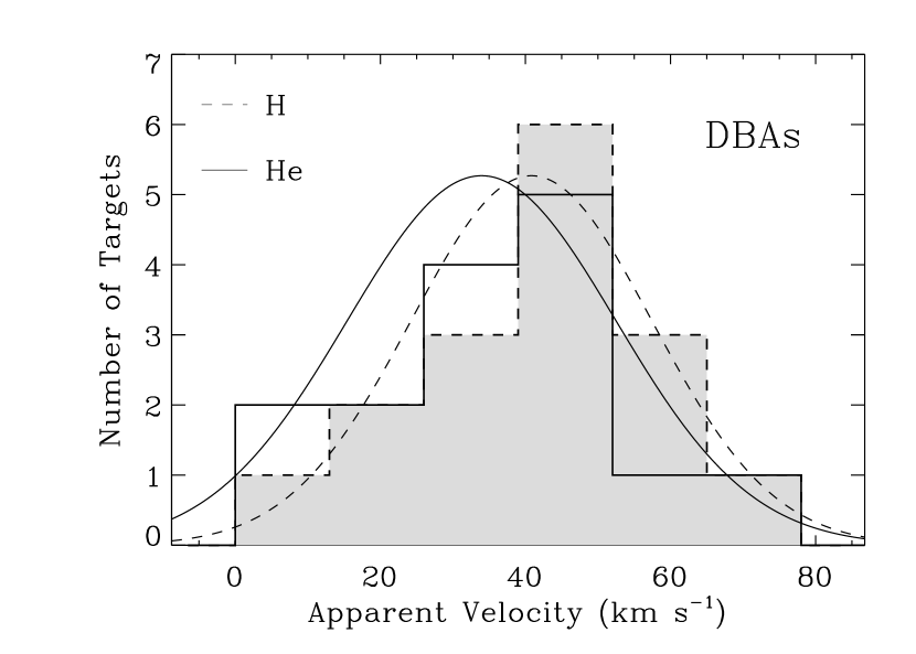
Figure 2.— Histograms of measured apparent velocities of H$\alpha$ $v_{\rm app}$ (dashed, filled) and of He I 5876 Å $v_{\rm app}^{\rm He}$ (solid, unfilled) for 16 DBAs. The bin size is 13 km s^-1. The dashed and solid curves are the Gaussian distributions used to determine Monte Carlo uncertainties for each sample. For H, $\langle v_{\rm app}\rangle_{\rm BI}=40.8\pm 4.7$ km s^-1 and $\sigma(v_{\rm app})_{\rm BI}=16.6$ km s^-1. For He, $\langle v_{\rm app}^{\rm He}\rangle_{\rm BI}=34.0\pm 5.0$ km s^-1 and $\sigma(v_{\rm app}^{\rm He})_{\rm BI}=18.6$ km s^-1.

For this sample, $\langle v_{\rm app}\rangle_{\rm BI}=40.8\pm 4.7$ km s^-1. We find that this is different from $\langle v_{\rm app}\rangle$ of DAs (32.57 km s^-1) at the 91% confidence level.

Given the small sample size, it is possible that a systematic uncertainty is skewing our result. For example, by chance kinematic substructures may not average out with only 16 targets as they would for a larger sample. As a check, we perform the following test: let us assume that the SPY DBAs have the same intrinsic mean mass as the SPY DAs. If we randomly pick 16 apparent velocities from the measured $v_{\rm app}$ distribution from Falcon et al. (2010), which contains 449 objects, how often is the $\langle v_{\rm app}\rangle_{\rm BI}$ of these 16 greater than $\langle v_{\rm app}\rangle_{\rm BI}=40.8$ km s^-1, our result for DBAs? Performing the random selection 30,000 times, we find that this false detection occurs 9% of the time. The synthetic biweights reproduce the $\langle v_{\rm app}\rangle$ of DAs with a standard deviation of 4.17 km s^-1. There is a rare but not insignificant possibility that our small sample size is fooling us.

Using spectroscopically determined $T_{\rm eff}$ from Voss et al. (2007), $\langle T_{\rm eff}\rangle_{\rm BI}=17,890\pm 250$ K. We use the mass-radius relation from our evolutionary models and interpolate to find $\langle M\rangle_{\rm BI}=0.71^{+0.04}_{-0.05}\,M_{\odot}$. This is larger than the mean mass for normal DAs determined using the same gravitational redshift method ($0.647^{+0.013}_{-0.014}\,M_{\odot}$; Falcon et al., 2010).

Though suggestive of a real difference in mean mass between the samples, this is not a stringent result. It remains plausible that no intrinsic difference exists. We can say, however, that the difference between $\langle v_{\rm app}\rangle_{\rm BI}$ of the DBAs and $\langle v_{\rm app}\rangle$ of normal DAs is no larger than 9.2 km s^-1, at the 95% confidence level. With a note of caution, because of the subleties in translating a mean apparent velocity to a mean mass, this corresponds to roughly $0.10\,M_{\odot}$.

Our $\langle M\rangle_{\rm BI}$ for DBAs is also larger than $0.62\pm 0.02\,M_{\odot}$, the biweight of the spectroscopic mass determinations for these targets from Voss et al. (2007). The value for the mean is the same as the biweight. We estimate the uncertainty using the same method as for our work, except that, since Voss et al. (2007) do not list individual uncertainties, we assign each mass an uncertainty equal to the standard deviation of the mass distribution. The biweight (and mean) spectroscopic mass of the 22 DBAs with $T_{\rm eff}\geq 16,500$ K from Bergeron et al. (2011) agrees well at $0.67\pm 0.02\,M_{\odot}$. For this value we use the mass uncertainties from Bergeron et al. (2011).

4.1.2 Analysis with the He I 5876 Å Line

By measuring $v_{\rm app}^{\rm He}$ – instead of that from the H$\alpha$ line – for the targets in our DBA sample, we find $\langle v_{\rm app}^{\rm He}\rangle_{\rm BI}=34.0\pm 5.0$ km s^-1. Table 2 lists individual measurements. As discussed in Section 3.6, this differs from the H$\alpha$ result by $6.9\pm 6.9$ km s^-1. It lies between the unity line and the theoretical blueshift derived from Dimitrijevic & Sahal-Brechot (1990) for plasma conditions corresponding to $T=16,500$ K and $n_{\rm e}=10^{17}$ cm^-3. This temperature is the lower limit of our sample, and this electron density is typical of WD photospheres.

4.2. DBs

We now use the He I 5876 Å line to perform the gravitational redshift method on DBs. We measure $v_{\rm app}^{\rm He}$ for 20 such WDs and find $\langle v_{\rm app}^{\rm He}\rangle_{\rm BI}=36.0\pm 5.6$ km s^-1. Table 3 lists individual measurements. After applying the correction for the blueshift due to pressure effects measured in Section 3.6, $\langle v_{\rm app}^{\rm He}\rangle_{\rm BI}=42.9\pm 8.9$ km s^-1. This uncertainty comes from adding the measured uncertainty and that of the correction in quadrature. Using $\langle T_{\rm eff}\rangle_{\rm BI}=20,570\pm 660$ K (Voss et al., 2007) with the corrected $\langle v_{\rm app}^{\rm He}\rangle_{\rm BI}$, we determine $\langle M\rangle_{\rm BI}=0.74^{+0.08}_{-0.09}\,M_{\odot}$.

This is different from $\langle v_{\rm app}\rangle$ of DAs at the 75% confidence level. The difference between $\langle v_{\rm app}^{\rm He}\rangle_{\rm BI}$ (with the blueshift correction) of the DBs and $\langle v_{\rm app}\rangle$ of DAs is $\leq 11.5$ km s^-1, at the 95% confidence level. This corresponds to roughly $0.12\,M_{\odot}$.

From Voss et al. (2007), we find $\langle M^{*}\rangle_{\rm BI}=0.58\pm 0.02\,M_{\odot}$ for these targets ($M^{*}$ denotes spectroscopic mass); the mean is $0.59\pm 0.02\,M_{\odot}$. The biweight spectroscopic mass of the 35 DBs with $T_{\rm eff}\geq 16,500$ K from Bergeron et al. (2011) is $0.63\pm 0.01\,M_{\odot}$; the mean is $0.64\pm 0.01\,M_{\odot}$. The mean of the 82 DBs with $T_{\rm eff}>16,000$ K from SDSS and whose spectra have S/N$\geq 20$ is $0.646\pm 0.006\,M_{\odot}$ (Kepler et al., 2010).

4.3. DBAs and DBs

As mentioned in Section 3.6, let us assume there are no fundamental differences between DBAs and DBs that would manifest as different mean masses. We can then apply the correction for the blueshift due to pressure effects, and we can improve both the precision and accuracy of our mean value determinations by combining the two samples. We do not discard the possibility, however, that the two groups are indeed fundamentally different.

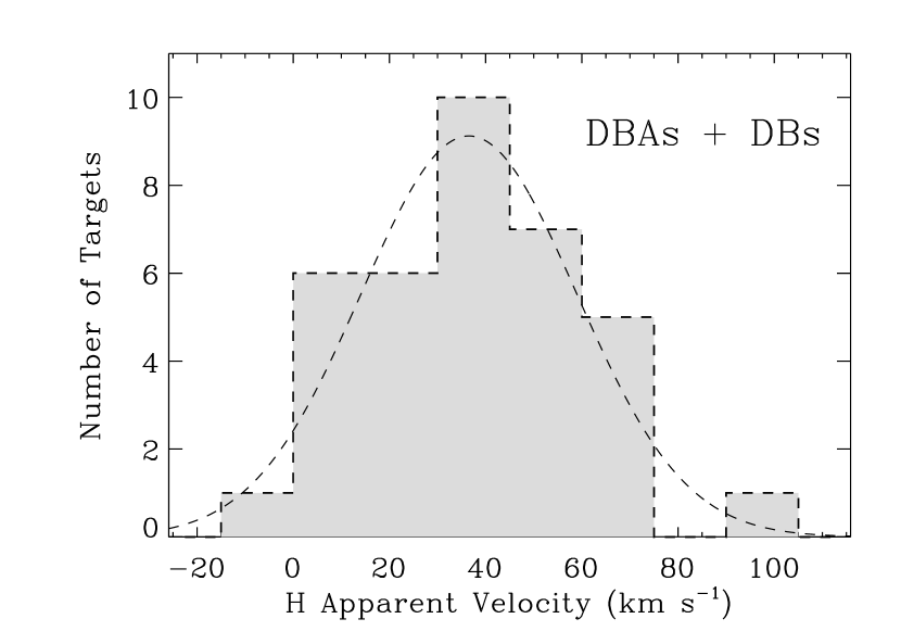
Figure 3.— Histogram of measured apparent velocities of the He I 5876 Å line $v_{\rm app}^{\rm He}$ for 36 DBAs and DBs (16 and 20, respectively) with a bin size is 15 km s^-1. The dashed curve is the Gaussian distribution used to determine Monte Carlo uncertainties. $\langle v_{\rm app}^{\rm He}\rangle_{\rm BI}=36.5\pm 3.9$ km s^-1 (before applying the correction discussed in Section 3.6) and $\sigma(v_{\rm app}^{\rm He})_{\rm BI}=22.4$ km s^-1.

Using the apparent velocity of the He I 5876 Å line for the combined sample of DBAs and DBs, we find $\langle v_{\rm app}^{\rm He}\rangle_{\rm BI}=36.5\pm 3.9$ km s^-1. Figure 3 shows the distribution of $v_{\rm app}^{\rm He}$. Applying the blueshift correction, $\langle v_{\rm app}^{\rm He}\rangle_{\rm BI}=43.4\pm 7.9$ km s^-1. Using $\langle T_{\rm eff}\rangle_{\rm BI}=19,260\pm 390$ K, we determine $\langle M\rangle_{\rm BI}=0.74^{+0.07}_{-0.08}\,M_{\odot}$.

This is different from the mean $v_{\rm app}$ of DAs at the 82% confidence level. The difference between $\langle v_{\rm app}^{\rm He}\rangle_{\rm BI}$ of this combined sample of DBAs + DBs and $\langle v_{\rm app}\rangle$ of DAs is $\leq 7.7$ km s^-1, at the 95% confidence level. This corresponds to roughly $0.08\,M_{\odot}$.

$\langle M^{*}\rangle_{\rm BI}=0.60\pm 0.02\,M_{\odot}$ for these targets using the spectroscopic masses from Voss et al. (2007). This is significantly lower than our determination. The biweight (and mean) spectroscopic mass of the 57 DBAs and DBs with $T_{\rm eff}\geq 16,500$ K from Bergeron et al. (2011) is $0.65\pm 0.01\,M_{\odot}$.

We list our derived $\langle v_{\rm app}\rangle_{\rm BI}$ in Table 4, denoting which samples use the He I 5876 Å line in lieu of the H$\alpha$ Balmer line. Since the $\langle v_{\rm app}\rangle_{\rm BI}$ values are entirely model independent, we list them apart from the $\langle M\rangle_{\rm BI}$ we determine. These are in Table 5. For comparison, we list the corresponding results for DAs from Falcon et al. (2010).

5. Conclusions

We measure the apparent velocity ($v_{\rm app}$) of the He I 5876 Å line for a sample of DBAs and compare it to that of the H$\alpha$ Balmer line. We find a difference of $6.9\pm 6.9$ km s^-1 in the average apparent velocities from the two line species, which we attribute to the blueshift of this He line due to pressure effects (e.g., Dimitrijevic & Sahal-Brechot, 1990) averaged over the sample. With assumptions one can apply this measured blueshift as a correction to other samples of helium-atmosphere WDs. We do so in order to investigate the average gravitational redshift of a sample of DBs for the first time.

Following the gravitational redshift method from Falcon et al. (2010), but using biweight estimators which are better suited for small sample sizes, we find $\langle v_{\rm g}\rangle_{\rm BI}=\langle v_{\rm app}\rangle_{\rm BI}=40.8\pm 4.7$ km s^-1 for 16 DBAs with $T_{\rm eff}\geq 16,500$ K from SPY. We translate this $\langle v_{\rm app}\rangle_{\rm BI}$ to a mass: $\langle M\rangle_{\rm BI}=0.71^{+0.04}_{-0.05}\,M_{\odot}$. Though different from the $\langle v_{\rm app}\rangle$ of DAs, 32.57 km s^-1, at the 91% confidence level and suggestive of a larger DBA mean mass than DA, $0.647^{+0.013}_{-0.014}\,M_{\odot}$ (Falcon et al., 2010), this is not a stringent result. We emphasize that the difference between $\langle v_{\rm app}\rangle_{\rm BI}$ of the DBAs and $\langle v_{\rm app}\rangle$ of normal DAs is no larger than 9.2 km s^-1, at the 95% confidence level; this corresponds to roughly $0.10\,M_{\odot}$. Our $\langle M\rangle_{\rm BI}$ for DBAs is also larger than the average of the spectroscopic mass determinations for these targets from Voss et al. (2007) at $0.62\pm 0.02\,M_{\odot}$. It agrees with the average mass of the 22 DBAs with $T_{\rm eff}\geq 16,500$ K from Bergeron et al. (2011) at $0.67\pm 0.02\,M_{\odot}$.

We use the He I 5876 Å line to conduct the first gravitational redshift investigation of a group of WDs without visible hydrogen lines. For 20 DBs from SPY, we find $\langle v_{\rm app}^{\rm He}\rangle_{\rm BI}=42.9\pm 8.9$ km s^-1 after applying the correction for our measured blueshift due to pressure effects. We determine $\langle M\rangle_{\rm BI}=0.74^{+0.08}_{-0.09}\,M_{\odot}$. The difference between $\langle v_{\rm app}^{\rm He}\rangle_{\rm BI}$ of the DBs and $\langle v_{\rm app}\rangle$ of DAs is $\leq 11.5$ km s^-1, at the 95% confidence level; this corresponds to roughly $0.12\,M_{\odot}$. The $\langle M\rangle_{\rm BI}$ is much larger than the average of the spectroscopic mass determinations from SPY, $0.58\pm 0.02\,M_{\odot}$. It is slightly larger than the average spectroscopic mass of DBs with $T_{\rm eff}>16,500$ K from Bergeron et al. (2011), $0.63\pm 0.01\,M_{\odot}$, and the mean of DBs with $T_{\rm eff}>16,000$ K from SDSS, $0.646\pm 0.006\,M_{\odot}$ (Kepler et al., 2010).

Combining our DBA and DB samples to group all WDs with helium-dominated atmospheres, we find $\langle v_{\rm app}^{\rm He}\rangle_{\rm BI}=43.4\pm 7.9$ km s^-1 (after the correction) and determine $\langle M\rangle_{\rm BI}=0.74^{+0.07}_{-0.08}\,M_{\odot}$. This differs from the $\langle v_{\rm app}\rangle$ of DAs at the 82% confidence level. The difference between $\langle v_{\rm app}^{\rm He}\rangle_{\rm BI}$ of the DBAs + DBs and $\langle v_{\rm app}\rangle$ of DAs is $\leq 7.7$ km s^-1 (roughly $0.08\,M_{\odot}$), at the 95% confidence level. Our $\langle M\rangle_{\rm BI}$ is much larger than the average spectroscopic mass of these targets from SPY at $0.60\pm 0.02\,M_{\odot}$ and slightly larger than the average spectroscopic mass of the DBAs and DBs with $T_{\rm eff}\geq 16,500$ K from Bergeron et al. (2011), $0.65\pm 0.01\,M_{\odot}$.

Given the small sample sizes, it is possible that system uncertainties are skewing our results due to the potential of kinematic substructures that may not average out. We estimate this to be unlikely, but a larger sample size is necessary to rule out these systematics.

Table 1H Apparent Velocity Measurements for DBAs

Target	Adopted		Date	Time	LSR	Observation
	$v_{\rm app}$	$\delta v_{\rm app}$			Correction	$v_{\rm app}$	$\delta v_{\rm app}$
	(km s-1)	(km s-1)	(UT)	(UT)	(km s-1)	(km s-1)	(km s-1)
HE 0025-0317	36.76	5.45	2000.07.17	07:52:34	27.319	36.76	1.80
HE 0110-5630	42.04	8.01	2002.09.25	07:28:16	-16.836	42.04	2.65
WD 0125-236	55.57	13.45	2002.09.30	04:23:09	-6.499	55.57	4.45
WD 0921+091	46.71	7.90	2001.04.07	00:55:54	-35.250	53.62	2.49
			2002.12.28	07:48:25	10.131	42.19	2.01
WD 0948+013	30.05	6.12	2001.01.10	01:31:21	-34.417	38.21	4.20
			2003.01.17	04:03:53	4.365	27.75	2.23
WD 1149-133	48.92	3.98	2000.07.13	23:40:32	-34.214	53.48	3.71
			2000.07.16	23:55:06	-33.761	47.18	2.29
HE 1207-2349	31.14	4.02	2002.02.23	07:41:20	12.910	43.82	6.79
			2002.02.24	07:11:53	12.571	30.51	1.52
EC 12438-1346	13.50	16.32	2000.07.15	00:27:35	-31.791	13.50	5.80
WD 1311+129	12.54	5.28	2001.06.20	01:47:22	-20.994	14.87	2.87
			2003.01.18	08:36:37	33.896	6.55	4.60
HE 1349-2305	15.58	5.91	2000.07.15	02:59:13	-28.698	15.58	1.95
WD 1421-011	56.32	11.11	2001.08.16	00:32:05	-19.271	56.32	3.67
WD 1557+192	52.12	4.68	2002.04.23	06:37:23	22.663	52.12	1.55
WD 1709+230	72.70	1.68	2002.09.04	00:10:33	-1.552	71.41	3.30
			2002.09.21	00:32:10	-1.091	73.80	3.05
WD 2154-437	41.92	4.20	2000.06.04	06:01:21	25.025	41.92	1.39
WD 2253-062	41.47	4.32	2000.06.01	08:50:29	37.290	37.64	3.38
			2000.06.06	08:07:23	37.293	44.02	2.51
HE 2334-4127	48.30	10.36	2002.09.14	02:03:49	-9.502	54.14	2.13
			2002.09.15	01:27:02	-9.859	39.11	2.67

Table 2He Apparent Velocity Measurements for DBAs

Target	Adopted		Date	Time	LSR	Observation
	$v_{\rm app}^{\rm He}$	$\delta v_{\rm app}^{\rm He}$			Correction	$v_{\rm app}^{\rm He}$	$\delta v_{\rm app}^{\rm He}$
	(km s-1)	(km s-1)	(UT)	(UT)	(km s-1)	(km s-1)	(km s-1)
HE 0025-0317	32.90	9.63	2000.07.17	07:52:34	27.319	32.90	4.54
HE 0110-5630	39.01	7.55	2002.09.25	07:28:16	-16.836	39.01	3.56
WD 0125-236	42.83	4.43	2002.09.30	04:23:09	-6.499	42.83	2.09
WD 0921+091	37.67	4.63	2001.04.07	00:55:54	-35.250	40.38	2.55
			2002.12.28	07:48:25	10.131	33.71	3.08
WD 0948+013	10.98	1.33	2001.01.10	01:31:21	-34.417	12.76	2.76
			2003.01.17	04:03:53	4.365	10.48	1.46
WD 1149-133	42.45	0.18	2000.07.13	23:40:32	-34.214	42.13	6.68
			2000.07.16	23:55:06	-33.761	42.51	2.68
HE 1207-2349	26.12	8.75	2002.02.23	07:41:20	12.910	20.72	3.80
			2002.02.24	07:11:53	12.571	33.22	4.36
EC 12438-1346	15.56	3.04	2000.07.15	00:27:35	-31.791	15.56	1.43
WD 1311+129	22.72	2.69	2001.06.20	01:47:22	-20.994	21.59	2.15
			2003.01.18	08:36:37	33.896	25.91	3.61
HE 1349-2305	10.49	3.72	2000.07.15	02:59:13	-28.698	10.49	1.75
WD 1421-011	66.97	8.23	2001.08.16	00:32:05	-19.271	66.97	3.88
WD 1557+192	61.57	3.28	2002.04.23	06:37:23	22.663	61.57	1.55
WD 1709+230	91.46	3.78	2002.09.04	00:10:33	-1.552	89.91	1.58
			2002.09.21	00:32:10	-1.091	96.09	2.73
WD 2154-437	30.39	4.40	2000.06.04	06:01:21	25.025	30.39	2.07
WD 2253-062	39.21	3.64	2000.06.01	08:50:29	37.290	37.50	1.36
			2000.06.06	08:07:23	37.293	43.11	2.06
HE 2334-4127	40.83	6.33	2002.09.14	02:03:49	-9.502	37.32	2.17
			2002.09.15	01:27:02	-9.859	46.56	2.77

Table 3He Apparent Velocity Measurements for DBs

Target	Adopted		Date	Time	LSR	Observation
	$v_{\rm app}^{\rm He}$	$\delta v_{\rm app}^{\rm He}$			Correction	$v_{\rm app}^{\rm He}$	$\delta v_{\rm app}^{\rm He}$
	(km s-1)	(km s-1)	(UT)	(UT)	(km s-1)	(km s-1)	(km s-1)
MCT 0149-2518	62.43	7.83	2002.09.27	08:32:10	-3.801	55.45	2.56
			2002.09.30	04:09:09	-4.575	66.83	2.03
WD 0158-160	47.19	3.20	2002.09.19	03:40:58	0.897	48.67	1.61
			2002.09.20	03:55:16	0.462	43.71	2.46
WD 0249-052	46.41	2.16	2002.09.20	07:09:51	9.064	50.32	3.97
			2002.12.31	02:03:00	-33.912	45.81	1.55
HE 0308-5635	63.79	6.87	2002.09.14	05:54:31	-12.226	63.79	2.75
WD 0349+015	8.96	2.21	2003.01.24	03:40:30	-38.561	8.96	0.88
HE 0417-5357	2.19	8.48	2000.07.15	10:16:58	-8.104	-6.21	3.25
			2000.07.18	09:37:59	-8.014	6.47	2.31
HE 0420-4748	57.29	0.06	2000.07.15	10:30:58	-6.686	57.37	2.83
			2000.07.18	10:19:41	-6.498	57.26	1.52
HE 0423-1434	55.50	5.98	2002.09.23	06:50:16	4.515	45.45	4.07
			2002.12.07	08:17:12	-22.990	57.28	1.71
WD 0615-591	1.94	0.61	2000.09.14	09:26:25	-13.891	1.322	2.83
			2001.04.08	01:04:56	-21.666	2.251	2.00
WD 0845-188	72.10	5.00	2001.12.18	07:32:37	2.566	70.29	1.79
			2001.12.29	07:17:47	-0.614	79.02	3.50
WD 1252-289	16.99	0.59	2000.04.21	04:49:17	-8.262	16.83	1.46
			2000.05.19	01:56:15	-20.292	18.10	3.85
WD 1326-037	51.82	6.61	2001.01.14	09:11:41	33.888	59.85	1.91
			2001.02.02	09:27:35	31.681	49.09	1.11
WD 1428-125	48.55	3.51	2000.07.06	02:51:29	-20.736	53.20	5.01
			2000.07.13	02:26:45	-22.017	47.22	2.68
WD 1445+152	-4.35	3.48	2002.04.23	05:32:37	11.695	-4.35	1.39
WD 1542+182	27.89	4.49	2002.04.23	08:22:15	20.960	27.89	1.80
WD 1612-111	45.50	2.48	2000.06.06	06:35:11	6.461	47.37	2.68
			2000.06.08	02:30:50	5.989	43.85	2.52
WD 2144-079	9.97	3.90	2000.05.17	09:50:49	40.410	11.93	1.75
			2000.05.19	09:58:26	40.360	6.080	2.47
WD 2234+064	19.21	4.19	2001.06.18	09:59:17	37.415	14.75	4.18
			2001.09.01	01:22:15	12.083	17.27	2.54
			2002.09.24	04:30:27	0.547	23.40	2.75
WD 2354+159	44.02	1.21	2002.09.04	06:44:23	18.606	43.46	1.43
			2002.09.13	04:25:56	14.692	45.33	2.19
WD 2354-305	34.30	10.00	2000.07.15	05:28:58	20.072	34.30	4.01

Table 4Biweight Apparent Velocities

Sample	Number of WDs	$\langle v_{\rm app}\rangle_{\rm BI}$	$\delta\langle v_{\rm app}\rangle_{\rm BI}$	$\sigma(v_{\rm app})_{\rm BI}$	$\langle\delta$$v_{\rm app}\rangle$	$\langle M/R\rangle_{\rm BI}$	$\delta\langle M/R\rangle_{\rm BI}$
		(km s-1)	(km s-1)	(km s-1)	(km s-1)	($M_{\odot}/R_{\odot}$)	($M_{\odot}/R_{\odot}$)
DBA	16	40.8	4.7	16.6	7.1	64.2	7.4
DBA (He)	16	34.0	5.0	18.6	4.7	53.4	7.8
DB (He)	20	42.9	8.9	23.9	4.1	67.4	13.9
DBA+DB (He)	36	43.4	7.9	22.4	4.5	68.9	12.5
DA	449	32.57	1.17	24.84	1.51	51.19	1.84

Table 5Biweight Masses

Sample	Number of WDs	$\langle v_{\rm app}\rangle_{\rm BI}$	$\delta$ $\langle v_{\rm app}\rangle_{\rm BI}$	$\langle T_{\rm eff}\rangle_{\rm BI}$	$\sigma(T_{\rm eff})_{\rm BI}$	$\langle M\rangle_{\rm BI}$	$\delta$ $\langle M\rangle_{\rm BI}$
		(km s-1)	(km s-1)	(K)	(K)	($M_{\odot}$)	($M_{\odot}$)
DBA	16	40.8	4.7	17890	1040	0.71	${}^{+0.04}_{-0.05}$
DB (He)	20	42.9	8.9	20570	3280	0.74	${}^{+0.08}_{-0.09}$
DBA+DB (He)	36	43.4	7.9	19260	2770	0.74	${}^{+0.07}_{-0.08}$
DA	449	32.57	1.17	19400	9950	0.647	${}^{+0.013}_{-0.014}$

References

- Bassalo & Cattani (1976) Bassalo, J. M., & Cattani, M. 1976, Journal of Physics B Atomic Molecular Physics, 9, L181
- Beauchamp & Wesemael (1998) Beauchamp, A., & Wesemael, F. 1998, ApJ, 496, 395
- Beauchamp et al. (1997) Beauchamp, A., Wesemael, F., & Bergeron, P. 1997, ApJS, 108, 559
- Beauchamp et al. (1999) Beauchamp, A., Wesemael, F., Bergeron, P., Fontaine, G., Saffer, R. A., Liebert, J., & Brassard, P. 1999, ApJ, 516, 887
- Beauchamp et al. (1996) Beauchamp, A., Wesemael, F., Bergeron, P., Liebert, J., & Saffer, R. A. 1996, in Astronomical Society of the Pacific Conference Series, Vol. 96, Hydrogen Deficient Stars, ed. C. S. Jeffery & U. Heber, 295–+
- Beers et al. (1990) Beers, T. C., Flynn, K., & Gebhardt, K. 1990, AJ, 100, 32
- Berg et al. (1962) Berg, H. F., Ali, A. W., Lincke, R., & Griem, H. R. 1962, Physical Review, 125, 199
- Bergeron et al. (1992) Bergeron, P., Saffer, R. A., & Liebert, J. 1992, ApJ, 394, 228
- Bergeron et al. (2011) Bergeron, P., Wesemael, F., Dufour, P., Beauchamp, A., Hunter, C., Saffer, R. A., Gianninas, A., Ruiz, M. T., Limoges, M.-M., Dufour, P., Fontaine, G., & Liebert, J. 2011, ApJ, 737, 28
- Bergeron et al. (1991) Bergeron, P., Wesemael, F., & Fontaine, G. 1991, ApJ, 367, 253
- Caballero (2009) Caballero, J. A. 2009, A&A, 507, 251
- Castanheira et al. (2006) Castanheira, B. G., Kepler, S. O., Handler, G., & Koester, D. 2006, A&A, 450, 331
- Dekker et al. (2000) Dekker, H., D’Odorico, S., Kaufer, A., Delabre, B., & Kotzlowski, H. 2000, in Society of Photo-Optical Instrumentation Engineers (SPIE) Conference Series, Vol. 4008, Society of Photo-Optical Instrumentation Engineers (SPIE) Conference Series, ed. M. Iye & A. F. Moorwood, 534–545
- Dimitrijevic & Sahal-Brechot (1990) Dimitrijevic, M. S., & Sahal-Brechot, S. 1990, A&AS, 82, 519
- Falcon et al. (2010) Falcon, R. E., Winget, D. E., Montgomery, M. H., & Williams, K. A. 2010, ApJ, 712, 585
- Farihi et al. (2005) Farihi, J., Becklin, E. E., & Zuckerman, B. 2005, ApJS, 161, 394
- Fich et al. (1989) Fich, M., Blitz, L., & Stark, A. A. 1989, ApJ, 342, 272
- Gilmore et al. (1989) Gilmore, G., Wyse, R. F. G., & Kuijken, K. 1989, ARA&A, 27, 555
- Grabowski et al. (1987) Grabowski, B., Halenka, J., & Madej, J. 1987, ApJ, 313, 750
- Greenstein & Trimble (1967) Greenstein, J. L., & Trimble, V. L. 1967, ApJ, 149, 283
- Griem et al. (1962) Griem, H. R., Kolb, A. C., & Shen, K. Y. 1962, ApJ, 135, 272
- Heading et al. (1992) Heading, D. J., Marangos, J. P., & Burgess, D. D. 1992, Journal of Physics B Atomic Molecular Physics, 25, 4745
- Hoard et al. (2007) Hoard, D. W., Wachter, S., Sturch, L. K., Widhalm, A. M., Weiler, K. P., Pretorius, M. L., Wellhouse, J. W., & Gibiansky, M. 2007, AJ, 134, 26
- Kepler et al. (2010) Kepler, S. O., Kleinman, S. J., Pelisoli, I., Peçanha, V., Diaz, M., Koester, D., Castanheira, B. G., & Nitta, A. 2010, in American Institute of Physics Conference Series, Vol. 1273, American Institute of Physics Conference Series, ed. K. Werner & T. Rauch, 19–24
- Kerr & Lynden-Bell (1986) Kerr, F. J., & Lynden-Bell, D. 1986, MNRAS, 221, 1023
- Kobilarov et al. (1989) Kobilarov, R., Konjević, N., & Popović, M. V. 1989, Phys. Rev. A, 40, 3871
- Koester (1987) Koester, D. 1987, ApJ, 322, 852
- Koester et al. (2005a) Koester, D., Napiwotzki, R., Voss, B., Homeier, D., & Reimers, D. 2005a, A&A, 439, 317
- Koester et al. (2005b) Koester, D., Rollenhagen, K., Napiwotzki, R., Voss, B., Christlieb, N., Homeier, D., & Reimers, D. 2005b, A&A, 432, 1025
- Koester et al. (1981) Koester, D., Schulz, H., & Wegner, G. 1981, A&A, 102, 331
- Koester et al. (2009) Koester, D., Voss, B., Napiwotzki, R., Christlieb, N., Homeier, D., Lisker, T., Reimers, D., & Heber, U. 2009, A&A, 505, 441
- Kuijken & Gilmore (1989) Kuijken, K., & Gilmore, G. 1989, MNRAS, 239, 605
- Limoges & Bergeron (2010) Limoges, M., & Bergeron, P. 2010, ApJ, 714, 1037
- Luyten (1949) Luyten, W. J. 1949, ApJ, 109, 528
- Montgomery et al. (1999) Montgomery, M. H., Klumpe, E. W., Winget, D. E., & Wood, M. A. 1999, ApJ, 525, 482
- Napiwotzki et al. (2001) Napiwotzki, R., Christlieb, N., Drechsel, H., Hagen, H.-J., Heber, U., Homeier, D., Karl, C., Koester, D., Leibundgut, B., Marsh, T. R., Moehler, S., Nelemans, G., Pauli, E.-M., Reimers, D., Renzini, A., & Yungelson, L. 2001, Astronomische Nachrichten, 322, 411
- Omar et al. (2006) Omar, B., Günter, S., Wierling, A., & Röpke, G. 2006, Phys. Rev. E, 73, 056405
- Pauli et al. (2006) Pauli, E.-M., Napiwotzki, R., Heber, U., Altmann, M., & Odenkirchen, M. 2006, A&A, 447, 173
- Pérez et al. (2003) Pérez, C., Santamarta, R., Rosa, M. I. D. L., & Mar, S. 2003, European Physical Journal D, 27, 73
- Reid (1996) Reid, I. N. 1996, AJ, 111, 2000
- Richter et al. (2007) Richter, R., Heber, U., & Napiwotzki, R. 2007, in Astronomical Society of the Pacific Conference Series, Vol. 372, 15th European Workshop on White Dwarfs, ed. R. Napiwotzki & M. R. Burleigh, 107–+
- Routly (1972) Routly, P. M. 1972, Publications of the U.S. Naval Observatory Second Series, 20, 1
- Shipman & Mehan (1976) Shipman, H. L., & Mehan, R. G. 1976, ApJ, 209, 205
- Voss et al. (2007) Voss, B., Koester, D., Napiwotzki, R., Christlieb, N., & Reimers, D. 2007, A&A, 470, 1079
- Wegner (1973) Wegner, G. 1973, MNRAS, 165, 271
- Wegner & Reid (1987) Wegner, G., & Reid, I. N. 1987, in IAU Colloq. 95: Second Conference on Faint Blue Stars, ed. A. G. D. Philip, D. S. Hayes, & J. W. Liebert, 649–651
- Wegner et al. (1989) Wegner, G., Reid, I. N., & McMahan, R. K. 1989, in Lecture Notes in Physics, Berlin Springer Verlag, Vol. 328, IAU Colloq. 114: White Dwarfs, ed. G. Wegner, 378–383
- Weidemann & Koester (1991) Weidemann, V., & Koester, D. 1991, A&A, 249, 389
- Zuckerman & Becklin (1992) Zuckerman, B., & Becklin, E. E. 1992, ApJ, 386, 260