A New Direction for Counting Perfect Matchings

Abstract

In this paper, we present a new exact algorithm for counting perfect matchings, which relies on neither inclusion-exclusion principle nor tree-decompositions. For any bipartite graph of $2n$ nodes and $\Delta n$ edges such that $\Delta\geq 3$, our algorithm runs with $O^{\ast}(2^{(1-1/O(\Delta\log\Delta))n})$ time and exponential space. Compared to the previous algorithms, it achieves a better time bound in the sense that the performance degradation to the increase of $\Delta$ is quite slower. The main idea of our algorithm is a new reduction to the problem of computing the cut-weight distribution of the input graph. The primary ingredient of this reduction is MacWilliams Identity derived from elementary coding theory. The whole of our algorithm is designed by combining that reduction with a non-trivial fast algorithm computing the cut-weight distribution. To the best of our knowledge, the approach posed in this paper is new and may be of independent interest.

1 Introduction

Counting perfect matchings in given input graph $G$ is recognized as one of hard combinatorial problems. In particular, the case that $G$ is bipartite has attracted much attention with its long history because of the relation to the computation of permanent, which is a characteristic value of matrices with many important applications. Since counting perfect matchings for bipartite graphs belongs to #P-complete, there seems to be no algorithm which runs within polynomial time for any input. Thus all of the previous studies lies on one (or more) of the following directions: Approximation, restriction of input graphs, or exact exponential algorithms. In this paper, we focus on the third line.

A seminal exponential-time algorithm for counting perfect matchings is Ryser’s one based on the inclusion-exclusion principle [25]. For any bipartite graph $G$ of $2n$ vertices, it counts perfect matchings with $O^{\ast}(2^{n})$ time and polynomial memory space. There has been several improvements following that work: Bax and Franklin have shown an algorithm running with $O^{\ast}(2^{(1-1/O(n^{2/3}\ln n))n})$ expected time and exponential space [3]. Servedio and Wan have given an algorithm with a time upper bound depending on the average degree $\Delta$ [26]. It achieves $O^{\ast}(2^{(1-1/O(\exp(\Delta)))n})$ time and polynomial space. Another approach to this problem is the usage of tree decompositions [2, 24]. By combining the fact that sparse graphs have a treewidth less than $(1-\epsilon)n$ for some constant $\epsilon$ (e.g., if $\Delta\leq 3$, $\epsilon\approx 5/6$ holds [10]), we can obtain an algorithm running $O^{\ast}(2^{(1-\epsilon)n})$ time. All of these algorithms break $O^{\ast}(2^{n})$-time barrier in some sense. However, during last 50 years, there has been proposed no algorithm achieving exponential-time speedup for any graph, which is a big open problem in this topic.

Our result presented in this paper can be put on the same line. The main contribution is to propose a new algorithm for counting perfect matchings. For any bipartite graph of $2n$ nodes and $\Delta n$ edges, it runs with $O^{\ast}(2^{(1-1/O(\Delta\log\Delta))n})$ time and exponential space. While this algorithm does not settle the open problem stated above, its speed-up factor becomes substantially closer to the exponential compared to the previous algorithms.

An important remark is that the approach we adopt is quite different from any previous solutions. It relies on neither inclusion-exclusion nor tree decomposition. Actually, the main idea is an extremely-simple reduction to the problem of computing the cut-weight distribution of the input graph. The precise construction of our algorithm can be summarized as follows:

• For any odd input bipartite graph $G$ of $2n$ nodes and $m$ edges, we can show that the number of $G$’s perfect matchings is equal to the number of elements with weight $m-n$ in its cycle space. In addition, for any bipartite graph $G$, it is possible to construct the odd bipartite graph $\tilde{G}$ which has the same number of perfect matchings as $G$, by adding a constant number of nodes.

• By utilizing the primal-dual relation between cycle space and cut space, we can reduce the problem of counting cycle-space elements with weight $m-n$ to computing the weight distribution of the cut space. The technical tool behind this reduction is the use of MacWilliams identity, which is a well-known theorem derived from elementary coding-theory. That identity provides the linear transformation (by so-called Krawtchouk matrices) that maps the weight-distribution vector of any cut space to the corresponding cycle space.

• Since the cardinality of the cut space is vertex-exponential, it is easy to construct a naive algorithm with $O^{\ast}(2^{2n})$ running time. We improve its running time by utilizing the bipartiteness property and a novel technique analogous to separator decompositions.

It should be noted that except for the last step, our approach is applicable to any graphs which may not be bipartite. Our reduction technique can be seen as an algebraic approach to the design of exact algorithms as considered in [7, 19], where several kinds of algebraic transformations are used for appropriate handling of target universes. To the best of our knowledge, this is the first attempt using the transformation by MacWilliams Identity (or equivalently Kratwtchouk matrices) for that objective.

The organization of the paper is as follows: We first presents several notions and definitions in Section 2, which includes an tiny tutorial of linear codes. Section 3 introduces our reduction to cut space. The algorithm to compute the cut-weight distribution is shown in Section 4 gives an algorithm computing the cut space. We mention the related work in Section 5, and finally conclude the paper in Section 6 with the open problems posed by our result.

2 Preliminaries from Coding Theory

A linear code $C$ over $\mathbb{F}_{2}$ defined by $n\times m$ matrix $M$ is the set of $m$-dimensional vectors as follows:

$$C=\{\boldsymbol{v}M|\boldsymbol{v}\in\mathbb{F}^{n}_{2}\}.$$

The matrix $M$ is called the generator matrix of $C$. By the definition, code $C$ is the linear subspace of $\mathbb{F}_{2}^{m}$ spanned by the row vectors of $M$. The rank of that subspace is denoted by $\mathit{rank}(M)$. Clearly, the number of codewords in $C$ (denoted by $|C|)$ is equal to $2^{\mathit{rank}(M)}$. A $(m,r)$-linear code is the one such that the length of codewords is $m$ and its rank is $r$.

Let $C$ be a linear code with generator matrix $M$. The parity check matrix $H$ of $C$ is the $m\times(m-\mathrm{rank}(M))$ matrix satisfying $H\boldsymbol{w}^{T}=\boldsymbol{0}$ for any codeword $\boldsymbol{w}\in C$. It is well-known that there is a duality between generator matrices and parity check matrices: For the code $C^{\perp}$ with generator matrix $H$, it is easily verified that $\boldsymbol{v}^{T}M=0$ holds for any $\boldsymbol{v}\in C^{\perp}$. That is, $M$ is the parity check matrix of $C^{\perp}$. Then the code $C^{\perp}$ is called the dual code of $C$. Obviously $\boldsymbol{v}^{T}\boldsymbol{v}^{\perp}=0$ holds for any $\boldsymbol{v}\in C$ and $\boldsymbol{v}^{\perp}\in C^{\perp}$. It implies that the dual code is the orthogonal complement of the primary code.

Given a codeword $\boldsymbol{w}$, the number of appearance of value $1$ in $\boldsymbol{w}$ is called the weight of $\boldsymbol{w}$. The weight distribution of a $(m,r)$-linear code $C$ is the $m$-dimensional vector whose $k$-th entry $W_{C}[k]$ is the number of codewords with weight $k$ in $C$. The weight distribution is often represented as the form of generating functions $F_{C}(x)=\sum_{w=0}^{m}W_{C}[w]x^{w}$. This function is called the weight-distribution polynomial of $C$. There is a well-known theorem providing a relationship between the weight-distribution polynomials of primary and dual codes:

Theorem 1 (MacWilliams Identity [20])

Let $C$ be a $(m,r)$-linear code over $\mathbb{F}_{2}$ and $C^{\perp}$ be its dual. Then, the following identity holds:

$$F_{C}(x)=\frac{1}{2^{r}}(1+x)^{m}F_{C^{\perp}}\left(\frac{1-x}{1+x}\right).$$

By comparing the coefficient of each monomial in both sides, we have the representation of $W_{C}[k]$ by a linear sum of the weight distribution of $C^{\perp}$:

$$W_{C}[i]=\frac{1}{2^{r}}\sum_{j=0}^{m}K_{m}(j,i)W_{C^{\perp}}[j],$$ (1)

where $K_{m}(j,i)$ is the value known as Krawtchouk polynomials, defined as follows:

$$K_{m}(j,i)=\sum_{k=0}^{m}(-1)^{k}{i\choose k}{{m-i}\choose{j-k}}.$$

3 Counting Perfect Matchings via Cycle Space

3.1 Cut and Cycle Spaces

In this section any arithmetic operation for elements of vectors and matrices is over field $\mathbb{F}_{2}$. Letting $G=(V,E)$ be an undirected graph with $n$ vertices $v_{1},v_{2},\cdots,v_{n}$ and $m$ edges $e_{1},e_{2},\cdots,e_{m}$, its incidence matrix $A^{G}=(A^{G}_{i,j})\in\mathbb{F}_{2}^{n\times m}$ is the one such that $A^{G}_{i,j}=1$ if and only if $v_{i}$ is incident to $e_{j}$ and $A^{G}_{i,j}=0$ otherwise. It is easy to check that the $i$-th row of $A^{G}$ is the 0-1 vector representation of the set of edges incident to $v_{i}$. Given a 0-1 (row) vector representation of $\boldsymbol{v}_{S}$ for a vertex subset $S\subseteq V$, $\boldsymbol{v}_{S}A^{G}$ is the cutset between $S$ and $V\setminus S$. It implies that the linear code defined by the generator matrix $A^{G}$ is equivalent to the family of edge subsets each of which represents a cutset, so-called the cut space of $G$.

As an well-known fact, the set of all cycles in $G$ induces a linear subspace of $\mathbb{F}_{2}^{m}$, where each element is a 0-1 vector representation of the edge set constituting one or more cycle(s). This subspace is called the cycle space of $G$. Note that the cycle space can be recognized as the set of all spanning even subgraphs (i.e., subgraphs where every vertex has an even degree). The matrix whose row is the basis of $G$’s cycle space is denoted by $B^{G}$. Similarly to the cut space, we regard the cycle space as a linear code defined by the generator matrix $B^{G}$. An important relationship between cut space and cycle space, stated below, is known:

Fact 1

The cycle space of $G$ is the orthogonal complement of the cut space of $G$.

This fact implies that the linear code associated with a cycle space is the dual code of that with the corresponding cut space, and vice versa. In the following argument, given an undirected graph $G$, $C(G)$ and $C^{\perp}(G)$ denote the linear codes defined by the generator matrices $B^{G}$ and $A^{G}$ respectively. We often use term “cutset of $G$” as the meaning of the codeword of $C(G)$ associated with that cutset. The same usage is also applied for cycle spaces.

3.2 From Cycle Space to Number of Perfect Matchings

Given an undirected graph $G=(V,E)$, we consider counting the number of perfect matchings of $G$. Since there is no perfect matching if the number of vertices is odd, we define $2n=|V|$. Let $m=|E|$ for short. The degree of vertex $v$ is denoted by $d(v)$. First we focus on the case that $G$ is an odd graph, i.e., a graph such that $d(v)$ is odd for any $v$ in $V$. The number of perfect matchings of odd graph $G$ is related to $G$’s cycle space by the following lemma.

Lemma 1

For any odd graph $G$, the number of perfect matchings in $G$ is equal to $W_{C(G)}[m-n]$.

Proof

Let $V=\{v_{0},v_{1},\cdots,v_{2n-1}\}$ be the set of vertices in $G$. We prove the lemma by defining a bijection between the set of codewords with weight $m-n$ and perfect matchings. More precisely, we prove that the complement (in terms of the edge set of $G$) of any codeword $\boldsymbol{w}$ in $C(G)$ with weight $m-n$ is a 1-factor (equivalent to a perfect matching). Let $G_{w}$ be a spanning even subgraph corresponding to $w$. The degree of $v_{i}\in V$ in $G_{w}$ is denoted by $d^{\prime}(v_{i})$. To prove that the complement of $G_{w}$ is a 1-factor, it suffices to show that $d^{\prime}(v_{i})=d(v_{i})-1$ holds for any $v_{i}\in V$. Suppose for contradiction that $d^{\prime}(v_{i})\neq d(v_{i})-1$ holds for some $v_{i}\in V$. Since $d^{\prime}(v_{i})\leq d(v_{i})$, $d(v_{i})$ is odd, and $d^{\prime}(v_{i})$ is even (recall $G_{w}$ is a spanning even subgraph of $G$), we have $d^{\prime}(v_{i})<d(v_{i})-1$. To make $\sum^{n-1}_{i=0}d^{\prime}(v_{i})=2(m-n)$ hold, there must exist another vertex $v_{j}$ satisfying $d^{\prime}(v_{j})>d(v_{j})-1\Rightarrow d(v_{j})=d^{\prime}(v_{j})$. It contradicts the fact that $d(v_{j})$ is odd.

Combining the lemma above and Theorem 1, we obtain the following corollary:

Corollary 1

Let $G$ be an arbitrary odd graph. There exists an algorithm to count the number of perfect matchings in $G$ with $O(m\tau(5m))$ time provided that the weight distribution $W_{C^{\perp}(G)}$ is available, where $m$ is the number of edges in $G$ and $\tau(x)$ be the time required for arithmetic operations of two $x$-bit integers.

Note that the absolute value of Krawtchouk polynomials has a trivial upper bound $|K_{m}(j,i)|\leq\mathrm{poly}(m){m\choose m/2}^{2}\leq 2^{2m+O(\log m)}$, and the number of all codewords of $C^{\perp}(G)$ is at most $2^{n}\leq 2^{m}$. Thus, the time required for each arithmetic operation in the right term of formula 1 is bounded by $\tau(5m)$.

3.3 Transformation to Odd Bipartite Graph

While the result in the previous subsection assumes that $G$ is an odd graph, that assumption can be easily removed. The fundamental idea is to construct the odd graph $\tilde{G}$ that has the same number of perfect matchings as $G$. While we only consider the case that $G$ is a bipartite graph in this paper, general graph can be handled similarly. Let $G=(V_{1}\cup V_{2},E)$, be an arbitrary bipartite graph such that $|V_{1}|=|V_{2}|=n$, and $V=V_{1}\cup V_{2}$ for short. The set of even-degree vertices in $V_{i}$ is denoted by $V^{\mathrm{even}}_{i}$ ($i\in\{1,2\}$). We can easily show the following lemma:

Lemma 2

The values of $|V^{\mathrm{even}}_{1}|$ and $|V^{\mathrm{even}}_{2}|$ have the same parity.

Proof

Assume that $|E|$ is odd. Since $\sum_{v\in V^{\mathrm{even}}_{i}}d(v)$ is even for any $i\in\{1,2\}$, $\sum_{v\in V\setminus V^{\mathrm{even}}_{i}}d(v)$ must be odd. Thus, $|V\setminus V^{\mathrm{even}}_{i}|$ is odd for any $i\in\{1,2\}$ because any node in $V\setminus V^{\mathrm{even}}_{i}$ has an odd degree. It implies that $|V^{\mathrm{even}}_{i}|$ is odd for any $\{1,2\}$. The case of even $|E|$ can be proved similarly.

The construction of $\tilde{G}$ is given as follows:

• Add two vertices $\tilde{v}_{i,1}$, and $\tilde{v}_{i,2}$ to $V_{i}$ for each $i\in\{1,2\}$.

• For each $i\in\{1,2\}$, connect each node in $V^{\mathrm{even}}_{i}$ with $\tilde{v}_{3-i,1}$, and $\tilde{v}_{3-i,1}$ with $\hat{v}_{i,2}$.

• If $d(\tilde{v}_{1,1})$ and $d(\tilde{v}_{2,1})$ are even, connect them. Recall that $d(\tilde{v}_{1,1})$ and $d(\tilde{v}_{2,1})$ have the same parity from Lemma 2.

An example of the construction is shown in Figure 1. For the constructed graph $\tilde{G}$, we have the following lemma.

Lemma 3

The graph $\tilde{G}$ is an odd bipartite graph, and has the same number of perfect matchings as $G$.

Proof

Any node in $\tilde{G}$ clearly has an odd degree. Let $M\subseteq\tilde{E}$ be any perfect matching of $\tilde{G}$. Since $\tilde{v}_{1,2}$ and $\tilde{v}_{2,2}$ is degree one, edges $\{\tilde{v}_{1,1},\tilde{v}_{2,2}\}$ and $\{\tilde{v}_{2,1},\tilde{v}_{1,2}\}$ are necessarily included in $M$. Then $M\setminus\{\{\tilde{v}_{1,1},\tilde{v}_{2,2}\},\{\tilde{v}_{2,1},\tilde{v}_{1,2}\}\}$ is a perfect matching of $G$. Conversely, given a perfect matching $M^{\prime}\subseteq E$ of $G$, $G\cup\{\{\tilde{v}_{1,1},\tilde{v}_{2,2}\},\{\tilde{v}_{2,1},\tilde{v}_{1,2}\}\}$ is a perfect matching of $\tilde{G}$. Thus, we have a one-to-one correspondence between the perfect matchings of $G$ and those of $\tilde{G}$. The lemma is proved.

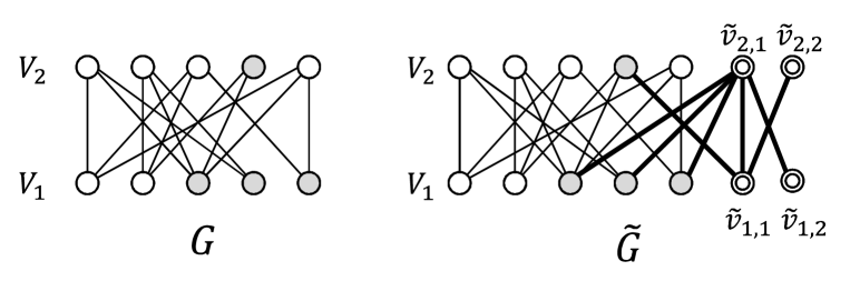
Figure 1: The construction of $\tilde{G}$

4 Computing Weight Distribution

As seen in the previous section, the computation of the cut weight distribution for graph $\tilde{G}$ induces the number of perfect matchings of $G$. Thus, in what follows, we focus on algorithms for computing the cut weight distribution.

The set of edges constituting a cut is associated with a partition of all vertices: A partition $(S,V\setminus S)$ of all vertices $V$ induces a cutset, which is the set of edges crossing between $S$ and $V\setminus S$. Thus we often use the sentence “partition $(S,V\setminus S)$ of $V$” as the meaning of the cut associated with that partition. We define $c(S,T)$ to be the set of edges crossing two disjoint subsets $S$ and $T$ ($S,T\subseteq V$). In particular, if $S$ (resp. $T$) is a singleton $\{v\}$, we use notation $c(v,T)$ (resp. $c(S,v)$).

While two different partitions can lead the same cutset (e.g., $(S,V\setminus S)$ and $(V\setminus S,S)$), it is well-known that exactly $2^{d}$ subsets induce the same cutset, where $d$ is the number of connected components of $G$ and equal to $n-\mathrm{rank}(A^{G})$. Thus, instead of computing $W_{C^{\perp}(G)}$, we rather consider the cut-weight distribution $W^{\prime}_{C^{\perp}(G)}$ over all partitions, that is, $W^{\prime}_{C^{\perp}(G)}[k]=|\{S\subseteq V||c(S,V\setminus S)|=k\}|$. It is easy to calculate $W_{C^{\perp}(G)}$ from $W^{\prime}_{C^{\perp}(G)}$ because of the relation of $W_{C^{\perp}(G)}=2^{-d}\cdot W^{\prime}_{C^{\perp}(G)}$.

4.1 $O^{\ast}(2^{n})$-time Algorithm

A straightforward way of computing $W^{\prime}_{C^{\perp}(G)}$ is to enumerate all partitions of $V$ with computing their weights, which trivially takes $O^{\ast}(2^{2n})$ time. In the case of bipartite graphs, we can reduce the time required for computing the cut-weight distribution. As a first step, this subsection proposes an $O^{\ast}(2^{n})$-time algorithm, which has the same performance as Ryser’s one [25] (in terms of the base of the exponential part). Further improvement of the running time is considered in the following subsection.

Let $G=(V_{1}\cup V_{2},E)$ be the input bipartite graph such that $|V_{1}|=|V_{2}|=n$ and $|E|=m$, and $V=V_{1}\cup V_{2}$ for short. For weight-distribution vector $W$ and integer value $x\in[-m,m]$, we define $\sigma_{x}(W)$ as the vector obtained by shifting each element of $W$ $x$ times. That is,

$$\sigma_{x}(W)[i]=\left\{\begin{array}[]{ll}0&\mbox{if $i<x$},\\ W[i-x]&\mbox{if $n-1\geq i\geq x$},\\ 0&\mbox{if $i\geq n+x$}.\end{array}\right.$$

Note that the case of $i<x$ or $i\geq n+x$ applies only when $x$ is positive or negative respectively. Let $V^{\prime}$ be a subset of $V$. We say that partition $(S,V\setminus S)$ is conditioned by a subset partition $(S^{\prime},V^{\prime}\setminus S^{\prime})$ if $S\supseteq S^{\prime}$ and $(V\setminus S)\supseteq(V^{\prime}\setminus S^{\prime})$ holds. Let $\mathcal{P}_{S^{\prime}|V^{\prime}}$ be the set of all partitions of $V$ conditioned by $(S^{\prime},V^{\prime}\setminus S^{\prime})$, and $W_{S^{\prime}|V^{\prime}}$ be the cut-weight distribution over all partitions in $\mathcal{P}_{S^{\prime}|V^{\prime}}$. Our algorithm relies on the fact that $W_{S|V_{1}}$ can be computed within polynomial time in $n$ provided that a partition $(S,V_{1}\setminus S)$ of $V_{1}$ is given. In the following argument, we introduce an arbitrary ordering $v_{0},v_{1},\cdots v_{n-1}$ of vertices in $V_{2}$. We define $V^{i}=\{v_{i},v_{i+1},\cdots v_{n-1}\}\cup V_{1}$. The lemma behind the correctness of our algorithm is stated below:

Lemma 4

For a given partition $(S,V_{1}\setminus S)$, let $l=|c(v_{i},V_{1}\setminus S)|-|c(v_{i},S)|$. Then $W_{S|V^{i+1}}=W_{S|V^{i}}+\sigma_{l}(W_{S|V^{i}})$ holds.

Proof

From the definition of $W_{S|V^{i}}$, $W_{S|V^{i+1}}=W_{S\cup\{v_{i}\}|V^{i}}+W_{S|V^{i}}$ clearly holds. Thus it suffices to show $W_{S\cup\{v_{i}\}|V^{i}}=\sigma_{l}(W_{S|V^{i}})$. Let $(S^{\prime},V\setminus S^{\prime})$ be a partition in $\mathcal{P}_{S|V^{i}}$, and $k$ be its weight. By adding $v_{i}$ to $S^{\prime}$, the weight increases by $l$. That is, the weight of partition $(S^{\prime}\cup\{v_{i}\},V\setminus(S^{\prime}\cup\{v_{i}\})$ is $k+l$. It implies a one-to-one correspondence between the partitions in $\mathcal{P}_{S|V^{i}}$ with weight $k$ and those in $\mathcal{P}_{S\cup\{v_{i}\}|V^{i}}$ with weight $k+l$. Hence we have $W_{S\cup\{v_{i}\}|V^{i}}[k+l]=W_{S|V^{i}}[k]$ for any $k$. It clearly follows $W_{S\cup\{v_{i}\}|V^{i}}=\sigma_{l}(W_{S|V^{i}})$. The lemma is proved. ∎

The recursive formula in Lemma 4 trivially allows us to compute $W_{S|V_{1}}=W_{S|V^{n-1}}$ within polynomial time in $n$. For the usefulness of the following argument, we encapsulate this recursion process by function shift shown in the pseudocode of Algorithm 1. Let $L:2^{V_{1}}\to\mathbb{Z}^{|V_{1}|}$ be the function such that $L(X)[i]=|c(v_{i},V_{1}\setminus X)|-|c(v_{i},X)|$ holds for any $v_{i}\in V_{2}$. Our $O^{\ast}(2^{n})$-time algorithm computes and sums up the values of shift($W_{X|V^{0}},L(X)$) over all partitions of $V_{1}$. That is, our algorithm computes the right side of the following equality:

$$W^{\prime}_{C^{\perp}(G)} =\sum_{S\subseteq V_{1}}\mathsf{shift}(W_{S|V^{0}},L(S)).$$ (2)

The correctness of this formula is obvious from the definition of $W_{S|V_{1}}$.

Theorem 2

There is an algorithm computing $W^{\prime}_{C^{\perp}(G)}$ with $O^{\ast}(2^{n})$ time.

Algorithm 1 shift: Function for computing $W_{X|V^{n-1}}$

1:	function shift($W,L$) $/\ast$ $W\in\mathbb{N}^{m}$ and , $L\in\mathbb{N}^{\ast}$ $\ast/$
2:		while $L$ is not empty do
3:			$l\leftarrow$ the head of $L$
4:			Remove the head of $L$
5:			$W\leftarrow W+\sigma_{l}(W)$
6:		endwhile
7:		return $W$

4.2 Function shift as a Linear Transformation

Before introducing the faster algorithm, we show several properties of Function shift. Let $H=\{h_{i,j}\}\in\mathbb{R}^{m\times m}$ be the matrix defined as $h_{i,j}=1$ if $j=i+1$ and $0$ otherwise. It is easy to check this matrix works as the operator $\sigma_{1}$, i.e., for any $m$-dimensional vector $W$, $WH^{x}=\sigma_{x}(W)$ holds. Hence we can describe function shift($W,L$) for a given sequence $L=(l_{0},l_{1},\cdots l_{n-1})$ as follows:

$$\mathsf{shift}(W,L) =W\left(\prod_{i=0}^{n-1}(H^{l_{i}}+I)\right),$$ (3)

where $I$ be the $m\times m$ identity matrix. We can obtain the following lemma:

Lemma 5

Letting $L$ and $L^{\prime}$ be two sequences of integers, and $W_{1},W_{2}\in\mathbb{N}^{m}$. Then the following properties hold:

1. $\sigma_{x}(\mathsf{shift}(W,L))=\mathsf{shift}(\sigma_{x}(W),L)$,

2. $\mathsf{shift}(\mathsf{shift}(W,L),L^{\prime})=\mathsf{shift}(W,L\circ L^{\prime})$,

3. $\sigma_{x}(W_{1}+W_{2})=\sigma_{x}(W_{1})+\sigma_{x}(W_{2})$, and $\mathsf{shift}(W_{1}+W_{2},L)=\mathsf{shift}(W_{1},L)+\mathsf{shift}(W_{2},L)$,

where $\circ$ is the concatenation of two sequences.

Proof

Since $\sigma_{x}(W)=\mathsf{shift}(W,(x))$, we can treat $\sigma_{x}$ equivalently to ${\sf shift}$. Clearly, Equation 3 implies that shift$(\ast,L)$ is a commutative linear transformation. Thus all properties obviously hold. ∎

4.3 Improving Running Time

In this subsection, we consider an improvement of $O^{\ast}(2^{n})$-time algorithm. The running time of the improved algorithm is $O^{\ast}(2^{(1-\frac{1}{5\Delta\log\Delta})n})$ and consumes exponential space, where $\Delta$ is the average degree of the input graph.

The underlying principle of the improved algorithm is very simple: Separating two smaller subproblems. Let $(T_{1},U_{1})$ be a partition of $V_{1}$ (i.e., $T_{1}=V_{1}\setminus U_{1}$) fixed by the algorithm, $N(U_{1})\subseteq V_{2}$ be the set of vertices adjacent to $U_{1}$, and $v_{0},v_{1},\cdots v_{n-1}$ be an arbitrary ordering of $V_{2}$ such that the last $|N(U_{1})|$ vertices correspond to $N(U_{1})$. The cardinality of $N(U_{1})$ is denoted by $h$ for short. Now we consider the situation where $U_{1}$ and $T_{1}$ are partitioned into $(X,U_{1}\setminus X)$ and $(Y,T_{1}\setminus Y)$. If we regards $X$ and $Y$ as variables, the first $n-h$ entries $(l_{0},l_{1},\cdots l_{n-h})$ of $L(X\cup Y)$ become a function of $X$, which are independent of the value of $Y$. In contrast, the last $h$ entries $(l_{n-h},l_{n-h+1},\cdots l_{n-1})$ are a function of both $X$ and $Y$. Consequently, by two appropriate functions $L_{T}:2^{|T_{1}|}\to\mathbb{Z}^{n-h}$ and $L_{U}:2^{T_{1}}\times 2^{U_{1}}\to\mathbb{Z}^{h}$, the sequence $L(X\cup Y)$ can be described as follows:

$$L(X,Y)=L_{T}(X)\circ L_{U}(X,Y).$$

Then the following lemma holds:

Lemma 6

$L_{U}(X,Y)=L_{U}(X,\emptyset)+L_{U}(\emptyset,Y)-L_{U}(\emptyset,\emptyset)$.

Proof

We prove $L_{U}(X,Y)[i]=L_{U}(X,\emptyset)[i]+L_{U}(\emptyset,Y)[i]-L(\emptyset,\emptyset)[i]$ for any $i$. Since $X\subseteq T_{1}$ and $Y\subseteq U_{1}$ are mutually disjoint, the sets of edges $c(v_{i},X)$ and $c(v_{i},Y)$ are mutually disjoint. Thus we have $|c(v_{i},X\cup Y)|=|c(v_{i},X)|+|c(v_{i},Y)|$. Similarly, we have $|c(v_{i},V_{1}\setminus(X\cup Y))|=|c(v_{i},(T_{1}\setminus X)\cup(U_{1}\setminus Y))|=|c(v_{i},(T_{1}\setminus X))|+|c(v_{i},(U_{1}\setminus Y))|$. Then we can obtain the following equality:

$$L_{U}(X,Y)[i] =|c(v_{i},V_{1}\setminus X\cup Y)|-|c(v_{i},(X\cup Y))|$$

$$=|c(v_{i},(T_{1}\setminus X))|-|c(v_{i},X)|+|c(v_{i},(U_{1}\setminus Y))|-|c(v_{i},Y)|$$

$$=|c(v_{i},(V_{1}\setminus X))|-|c(v_{i},T_{1})|-|c(v_{i},X)|+|c(v_{i},(V_{1}\setminus Y))|-|c(v_{i},U_{1})|-|c(v_{i},Y)|$$

$$=L_{U}(X,\emptyset)[i]+L_{U}(\emptyset,Y)[i]-|c(v_{i},T_{1})|-|c(v_{i},U_{1})|$$

$$=L_{U}(X,\emptyset)[i]+L_{U}(\emptyset,Y)[i]-|c(v_{i},T_{1}\cup U_{1})|$$

$$=L_{U}(X,\emptyset)[i]+L_{U}(\emptyset,Y)[i]-L_{U}(\emptyset,\emptyset)[i].$$

The lemma is proved. ∎

The improved algorithm runs as follows:

• (Step 1) We divide all partitions of $T_{1}$ into several classes $\mathcal{C}_{0},\mathcal{C}_{1},\cdots\mathcal{C}_{x}$ such that for any two partitions $(X_{1},T_{1}\setminus X_{1})$ and $(X_{2},T_{1}\setminus X_{2})$ in the same class, $L_{U}(X_{1},\emptyset)=L(X_{2},\emptyset)$ holds.

• (Step 2) For each $i\in[1,x]$, we compute weight distribution $W_{i}=\sum_{(X,T_{1}\setminus X)\in\mathcal{C}_{i}}W_{X|V^{n-h-1}}$.

  (Note that $W_{i}=\sum_{(X,T_{1}\setminus X)\in\mathcal{C}_{i}}\mathsf{shift}(W_{X|V^{0}},L_{T}(X))$ holds.)

• (Step 3) Let $L(i)$ be the value of $L_{U}(X,\emptyset)$ associated with class $\mathcal{C}_{i}$ and $c_{Y}=|c(Y,V_{2})|$ for short. For each $i\in[0,x]$ and each partition $(Y,U_{1}\setminus Y)$ of $U_{1}$, we compute $L_{U}(i,Y)=L(i)+L_{U}(\emptyset,Y)-L_{U}(\emptyset,\emptyset)$ and shift($\sigma_{c_{Y}}(W_{i}),L_{U}(i,Y)$). The sum of all the values returned by function shift is the output of the algorithm.

We can show the following lemma, which directly leads the correctness of the algorithm:

Lemma 7

$W^{\prime}_{C^{\perp}(G)}=\sum_{i=1}^{x}\sum_{Y\subseteq U_{1}}\mathsf{shift}(\sigma_{c_{Y}}(W_{i}),L_{U}(i,Y))$.

Proof

Since $W_{X|V^{0}}$ is the distribution over singleton $\{(X,V^{0}\setminus X)\}$, we have $W_{X|V^{0}}[i]=1$ for $i=|c(X,V^{0}\setminus X)|$ and $0$ otherwise. Thus, we have $\sigma_{c_{Y}}(W_{X|V^{0}})[i]=1$ for $i=|c(X,V^{0}\setminus X)|+c_{Y}$ and $0$ otherwise. Since $|c(X,V^{0}\setminus X)|+c_{Y}=|c(X\cup Y,V\setminus(X\cup Y))|$ holds, we obtain

$$\sigma_{c(Y)}(W_{X|V^{0}}) =W_{X\cup Y|V^{0}}.$$ (4)

By using this equation, Lemma 5 and 7, we can obtain the following equality:

$$\sum_{i=1}^{x}\sum_{Y\subseteq U_{1}}\mathsf{shift}(\sigma_{c_{Y}}(W_{i}),L_{U}(i,Y))$$

$$=\sum_{i=1}^{x}\sum_{Y\subseteq U_{1}}\mathsf{shift}\left(\sigma_{c_{Y}}\left(\sum_{(X,T_{1}\setminus X)\in\mathcal{C}_{i}}W_{X|V^{n-h-1}}\right),L_{U}(i,Y)\right)$$

$$=\sum_{i=1}^{x}\sum_{Y\subseteq U_{1}}\sum_{(X,T_{1}\setminus X)\in\mathcal{C}_{i}}\mathsf{shift}\left(\sigma_{c_{Y}}(W_{X|V^{n-h-1}}),L_{U}(X,Y)\right)$$

$$=\sum_{i=1}^{x}\sum_{Y\subseteq U_{1}}\sum_{(X,T_{1}\setminus X)\in\mathcal{C}_{i}}\mathsf{shift}\left(\sigma_{c_{Y}}(\mathsf{shift}(W_{X|V^{0}},L_{T}(X))),L_{U}(X,Y)\right)$$

$$=\sum_{i=1}^{x}\sum_{Y\subseteq U_{1}}\sum_{(X,T_{1}\setminus X)\in\mathcal{C}_{i}}\mathsf{shift}\left(\mathsf{shift}(\sigma_{c_{Y}}(W_{X|V^{0}}),L_{T}(X)),L_{U}(X,Y)\right)$$

$$=\sum_{i=1}^{x}\sum_{Y\subseteq U_{1}}\sum_{(X,T_{1}\setminus X)\in\mathcal{C}_{i}}\mathsf{shift}\left(\sigma_{c_{Y}}(W_{X|V^{0}}),L_{T}(X)\circ L_{U}(X,Y)\right)$$

$$=\sum_{X\subseteq T_{1},Y\subseteq U_{1}}\mathsf{shift}(W_{X\cup Y|V^{0}},L(X\cup Y))$$

$$=W^{\prime}_{C^{\perp}(G)}.$$

The lemma is proved. ∎

We focus on the running time of the algorithm. Clearly the first and second steps of the algorithm take $O^{\ast}(2^{n-|U_{1}|})$ time respectively. The third step requires time of $O^{\ast}(x2^{|U_{1}|})$. Thus the total running time is $O^{\ast}(2^{n-|U_{1}|}+x2^{|U_{1}|})$.

How small can we bound $x$? Clearly, it is upper bounded by the size of the domain of $L_{U}(X)$. From the definition, the value of $L_{U}(X)[i-(n-h)]$ can take $d(v_{i})+1$ different values for any $v_{i}\in N(U_{1})$. It follows $x\leq\prod_{v_{i}\in N(U_{1})}(d(v_{i})+1)$. By applying the arithmetic mean-geometric mean inequality, we can further bound $x$ by $((\sum_{v_{i}\in N(U_{1})}(d(v_{i})+1))/|N(U_{1})|)^{|N(U_{1})|}$. Letting $\Delta_{X}$ be the average degree over $X\subseteq V$ in $G$, we have

$$x \leq(\Delta_{N(U_{1})}+1)^{|N(U_{1})|}.$$ (5)

We consider how to choose $U_{1}$. Letting $\Delta$ be the average degree of $G$, $V_{1}$ contains a subset $X$ of $n/5$ vertices whose degrees are at most $5\Delta/4$. We choose $n/(5\Delta\log\Delta)$ vertices from $X$ as $U_{1}$. For that choice we have $|N(U_{1})|\leq n/(4\log\Delta)$. Since $|N(U_{1})|\Delta_{N(U_{1})}\leq\Delta n$ holds, we obtain $\Delta_{N(U_{1})}\leq 4\Delta\log\Delta$. By assigning this bound to Inequality 5, we obtain

$$x\leq(4\Delta\log\Delta+1)^{\frac{n}{4\log\Delta}}\leq(4\Delta^{2})^{\frac{n}{4\log\Delta}}=O(2^{\frac{5n}{6}})$$

Consequently, it follows that the running time of our algorithm is $O^{\ast}(2^{(1-\frac{1}{5\Delta\log\Delta})n})$.

Theorem 3

There is an an algorithm for counting perfect matchings of bipartite graphs which runs with $O^{\ast}(2^{(1-\frac{1}{5\Delta\log\Delta})n})$ time and exponential space.

5 Related Work

As seen in the introduction, we have roughly three lines about the studies on counting perfect matchings. We introduce the related work along them respectively.

There has been proposed two different approach for approximating the number of perfect matchings. The first one is the Markov-chain Monte Carlo method, which gives a fully-polynomial randomized approximation scheme (FPRAS) for counting perfect matchings [14, 15, 4]. The second one is a randomized averaging of the determinant [12, 16, 8]. The fastest approximation algorithm on this approach is one by Chien et.al. [8], which runs with $O(1.2^{n})$ time. It is still an open problem whether there exists a FPRAS following this approach or not.

The second line is the algorithm design for restricted inputs. A seminal work on this line is a polynomial-time exact counting algorithm for planar graphs [17]. As other restrictions, graphs of bounded genus [11, 27] or bounded treewidth [2, 24], and chordal graphs with its subclass [23] are considered.

About the line of exact algorithms, we have already mentioned the results for bipartite graphs in the introduction. Thus we introduce only the work on counting perfect matchings for general graphs. A first result breaking the trivial $O^{\ast}(2^{m})$-time bound is one by Björklund and Husfeldt [6], which has shown two algorithms: The first one runs with $O^{\ast}(2^{2n})$ time and polynomial space, and the second rounds with $O^{\ast}(1.733^{2n})$ time and exponential space. These algorithms are similar with our result in the sense that it also reduces the problem into a counting over a different universe. A number of the following studies improve this bound [18, 21, 1, 22, 5]. The most recent and fastest one is the algorithm by Björklund [5], which achieves the same running time as Ryser’s algorithm (that is, currently we do not find the difference of inherent difficulty between bipartite and general graphs). About time complexity, Dell et.al. [9] has shown that any algorithm has an instance of $m$ edges incurring $\Omega(exp(m/\log m))$ time if we believe that a counting version of the Exponential Time Hypothesis [13] is true.

6 Concluding Remarks

In this paper, we presented a new algorithm for the problem of counting perfect matchings, which has an improved time bound depending on the average degree $\Delta$ of the input graph. Compared to previous results, our algorithm runs faster for many cases. In particular, the performance degradation to the increase of $\Delta$ is quite slower than the previous algorithms. The main idea of our algorithm is a new reduction to computing the cut-weight distribution of the input graph. Our algorithm is designed by combining this reduction with a novel algorithm for the computation of cut-weight distribution. The approach itself is quite new, and may be of independent interest. Finally, we conclude the paper with several open problems related to our approach.

• Can we achieve the running time exponentially faster than Ryser’s one by designing a faster algorithm computing cut-weight distribution?

• The reduction part of our result is directly applicable to any graph (which may not be bipartite). Can we use the reduction to obtain a faster algorithm for general graphs? Actually, letting $I(G)$ be the independent sets of the input graph $G$, we can easily obtain an algorithm with $O^{\ast}(2^{2n-|I(G)|})$ running time by regarding $G$ as a ”quasi” bipartite graph of two vertex sets $I(G)$ and $V\setminus I(G)$ and applying our $O^{\ast}(2^{n})$-time algorithm, which gives the same performance as the algorithm by [1].

• Is it possible to design a faster FPRAS for counting perfect matchings based on our method? Note that an $(1+\epsilon)$-approximation of the cut-weight distribution trivially induces an $(1+\epsilon)$-approximation of the number of perfect matchings because of the linearity of the transformation.

• Computing cut-weight distribution is a special case of the counting version of 2-CSP, which is addressed by Williams [28]. In this sense, our reduction gives a new linkage from counting perfect matchings to CSP. Can we use this linkage for obtaining some new complexity result around those problems?

• Can we apply the same technique to other combinatorial problems? Interestingly, there has been proposed a variety of MacWilliams-style Identities in the field of the coding theory. We may find a useful transformation from those resources. In addition, it may be an interesting approach to focus on the primal-dual relationship of two universes. Can we design a kind of primal-dual algorithms for counting problems?

References

- [1] O. Amini, F. V. Fomin, and S. Saurabh. Counting subgraphs via homomorphisms. In Proc. of the 36th international colloquium conference on Automata, languages and programming (ICALP), pages 71–82, 2009.
- [2] S. Arnborg, J. Lagergren, and D.f Seese. Easy problems for tree-decomposable graphs. J. Algorithms, 12:308–340, 1991.
- [3] E. T. Bax and J. Franklin. A permanent algorithm with expected speedup for 0-1 matrices. Algorithmica, 32(1):157–162, 2002.
- [4] I. Bezáková, D. Štefankovič, V. V. Vazirani, and E. Vigoda. Accelerating simulated annealing for the permanent and combinatorial counting problems. In Proc. of the 17th annual ACM-SIAM symposium on Discrete algorithm (SODA), pages 900–907, 2006.
- [5] A. Björklund. Counting perfect matchings as fast as ryser. In Proc of ACM-SIAM Symposium on Discrete Algorithms (SODA), pages 914–921, 2012.
- [6] A. Björklund and T. Husfeldt. Exact algorithms for exact satisfiability and number of perfect matchings. Algorithmica, 52:226–249, 2008.
- [7] A. Björklund, T. Husfeldt, P. Kaski, and M. Koivisto. Fourier meets möbius: fast subset convolution. In Proc. of the 39th annual ACM symposium on Theory of computing (STOC), pages 67–74, 2007.
- [8] S. Chien, L. Rasmussen, and A. Sinclair. Clifford algebras and approximating the permanent. In Proc. of the 34th annual ACM symposium on Theory of computing (STOC), pages 222–231, 2002.
- [9] H. Dell, T. Husfeldt, and M. Wahlén. Exponential time complexity of the permanent and the tutte polynomial. In Proc. of the 37th international colloquium conference on Automata, languages and programming (ICALP), volume LNCS 6198, pages 426–437, 2010.
- [10] F. V. Fomin and K. Høie. Pathwidth of cubic graphs and exact algorithms. Information Processing Letters, 97:191–196, March 2006.
- [11] A. Galluccio and M. Loebl. On the theory of pfaffian orientations. i. perfect matchings and permanents. Electronic Journal of Combinatorics, 6, 1999.
- [12] C. D. Godsil and I. Gutman. On the matching polynomial of a graph. In Algebraic Methods in Graph Theory, pages 241–249. 1981.
- [13] R. Impagliazzo, R. Paturi, and F. Zane. Which problems have strongly exponential complexity? Journal of Computer and System Sciences, 63(4):512–530, 2001.
- [14] M. Jerrum and A. Sinclair. Approximating the permanent. SIAM Journal on Computing, 18:1149–1178, 1989.
- [15] M. Jerrum, A. Sinclair, and E. Vigoda. A polynomial-time approximation algorithm for the permanent of a matrix with nonnegative entries. Journal of the ACM, 51:671–697, 2004.
- [16] N. Karmarkar, R. Karp, R. Lipton, L. Lovász, and M. Luby. A monte-carlo algorithm for estimating the permanent. SIAM Journal on Computing, 22:284–293, 1993.
- [17] P. Kasteleyn. Graph theory and crystal physics. In Graph Theory and Theoretical Physics, pages 43–110. Academic Press, 1967.
- [18] M. Koivisto. Partitioning into sets of bounded cardinality. In Proc. of 4th International Workshop on Parameterized and Exact Computation (IWPEC), volume LNCS 5917, pages 258–263, 2009.
- [19] D. Lokshtanov and J. Nederlof. Saving space by algebraization. In Proc. of the 42th annual ACM symposium on Theory of computing (STOC), pages 321–330, 2010.
- [20] F. J. MacWilliams and N. J. A. Sloane. The Theory of Error-Correcting Codes. Elsevier, 1977.
- [21] J. Nederlof. Inclusion excluion for hard problems, 2008.
- [22] J. Nederlof. Fast polynomial-space algorithms using mobius inversion: Improving on steiner tree and related problems. available at http://www.uib.no/People/jne061/Steinerfull.pdf, 2010.
- [23] Y. Okamoto, R. Uehara, and T. Uno. Counting the number of matchings in chordal and chordal bipartite graph classes. In Proc. of 35th International Workshop on Graph-Theoretic Concepts in Computer Science (WG), pages 296–307, 2009.
- [24] J. M. M. Rooij, H. L. Bodlaender, and P. Rossmanith. Dynamic programming on tree decompositions using generalised fast subset convolution. In Proc. of 17th Annual European Symposium on Algorithms (ESA), pages 566–577, 2009.
- [25] H.J. Ryser. Combinatorial Mathematics. The Carus mathematical monographs. Mathematical Association of America, 1963.
- [26] R. A. Servedio and A. Wan. Computing sparse permanents faster. Information Processing. Letters, 96:89–92, November 2005.
- [27] G. Tesler. Matchings in graphs on non-orientable surfaces. Journal of Combinatrial Theory Series B, 78:198–231, 2000.
- [28] R. Williams. A new algorithm for optimal 2-constraint satisfaction and its implications. Theoretical Computer Science, 348(2):357–365, dec 2005.