Observational constraints on conformal time symmetry, missing matter and double dark energy

Abstract

The current concordance model of cosmology is dominated by two mysterious ingredients: dark matter and dark energy. In this paper, we explore the possibility that, in fact, there exist two dark-energy components: the cosmological constant $\Lambda$, with equation-of-state parameter $w_{\Lambda}=-1$, and a ‘missing matter’ component $X$ with $w_{X}=-2/3$, which we introduce here to allow the evolution of the universal scale factor as a function of conformal time to exhibit a symmetry that relates the big bang to the future conformal singularity, such as in Penrose’s conformal cyclic cosmology. Using recent cosmological observations, we constrain the present-day energy density of missing matter to be $\Omega_{X,0}=-0.034\pm 0.075$. This is consistent with the standard $\Lambda$CDM model, but constraints on the energy densities of all the components are considerably broadened by the introduction of missing matter; significant relative probability exists even for $\Omega_{X,0}\sim 0.1$, and so the presence of a missing matter component cannot be ruled out. As a result, a Bayesian model selection analysis only slightly disfavours its introduction by 1.1 log-units of evidence. Foregoing our symmetry requirement on the conformal time evolution of the universe, we extend our analysis by allowing $w_{X}$ to be a free parameter. For this more generic ‘double dark energy’ model, we find $w_{X}=-1.01\pm 0.16$ and $\Omega_{X,0}=-0.10\pm 0.56$, which is again consistent with the standard $\Lambda$CDM model, although once more the posterior distributions are sufficiently broad that the existence of a second dark-energy component cannot be ruled out. The model including the second dark energy component also has an equivalent Bayesian evidence to $\Lambda$CDM, within the estimation error, and is indistinguishable according to the Jeffreys guideline.

1 Introduction

Over the past two decades, cosmological observations have confirmed that the background expansion of the universe is accelerating [2, 1]. This remarkable phenomenon is usually explained by assuming the existence of a single dark-energy component, often modelled as a perfect fluid with a (generally time-dependent) equation-of-state parameter $w(z)$ that results in it exhibiting a negative pressure. The simplest form of dark energy is a cosmological constant $\Lambda$, which corresponds to a constant equation of state $w_{\Lambda}=-1$. Together with cold dark matter, which is key to explaining the evolution of structure in the universe, the cosmological constant gives rise to the standard $\Lambda$CDM model, which provides a good fit to existing cosmological observations. Nonetheless, there have been a large number of other exotic forms of matter proposed to provide alternative explanations for the current accelerating universal expansion [3, 4], including, for example, topological defects [5].

In this paper, we remain focussed on the $\Lambda$CDM model, but with the inclusion of a second, additional, dark energy component, having a different equation of state parameter. One of the motivations for exploring such a possibility arises from Penrose’s ‘conformal cyclic cosmology’ (CCC) model [6], which posits a cyclic universe in which the ultimate infinitely expanded state of one phase (or ‘aeon’) is identified with the initial singularity of the next. One way of realising such a model is to relate the future conformal singularity to the big bang, which leads one to investigate the symmetries of the Friedmann equations when written in terms of conformal time. Interestingly, as we will show, one finds that if the evolution of the universal scale factor $a$ is to have an appropriate symmetry in conformal time, one requires the existence of an additional component with equation-of-state $w=-\tfrac{2}{3}$.

Indeed, even without the above considerations, the standard form of the Friedmann equation written in terms of cosmic time hints at such a hitherto neglected additional component. For a homogeneous and isotropic universe described by the Friedmann–Robertson–Walker (FRW) metric, the Friedmann equation describing the dynamical evolution of the scale factor $a(t)$ can be written as

$$\left(\frac{H}{H_{0}}\right)^{2}=\sum_{i}\Omega_{i,0}\,a^{-3(1+w_{i})},$$ (1.1)

where $H=\dot{a}/a$ is the Hubble parameter (the dot denotes differentiation with respect to cosmic time $t$), and the energy density $\rho_{i}$ of each of the constituent components of the universe is taken into account through a corresponding density parameter $\Omega_{i,0}=8\pi G\rho_{i,0}/(3H_{0}^{2})$. The equation-of-state parameters are $w_{i}$, which we will assume throughout to be time-independent. The summation in (1.1) also includes the curvature density parameter $\Omega_{k,0}$, so that $\sum_{i}\Omega_{i,0}=1$.

In the $\Lambda$CDM model, the total density parameter is usually taken to comprise of contributions from radiation ($w=\frac{1}{3}$), matter (typically modelled as dust with $w=0$), curvature ($w=-\frac{1}{3}$), and the cosmological constant ($w=-1$). These are listed in Table 1, in which one can see an obvious ‘gap’ that we term ‘missing matter’ with $w=-\frac{2}{3}$. Interestingly, forms of matter have been proposed for which $w=-\frac{2}{3}$, such as domain walls [8, 7, 9], or particular scalar field models [10].

$w_{i}$	component	$\Omega_{i}$
$1/3$	radiation	$\Omega_{\rm r}$
$0$	matter (dust)	$\Omega_{\rm m}$
$-1/3$	curvature	$\Omega_{k}$
$-2/3$	missing matter ?	$\Omega_{X}$
$-1$	cosmological constant	$\Omega_{\Lambda}$

Table 1: Canonical equation-of-state parameters for different constituents of the universe.

It should be noted, of course, that the true equation-of-state parameters for matter and radiation will, in general, differ from the canonical values listed in Table 1 (although these values are assumed in most cosmological analyses). For example, non-relativistic matter does not have exactly zero pressure ($w=0$), but a pressure proportional to $(v/c)^{2}$. Similarly, relativistic particles such as massive neutrinos have an equation-of-state parameter slightly less than $w=\frac{1}{3}$, which changes with cosmic epoch. Nonetheless, these deviations from the canonical values are small and the equation-of-state parameters for curvature and a pure cosmological constant are fixed to the values listed in Table 1. Hence the suggestion of a missing component remains a distinguishable (distinct) possibility.

Once one admits the possibility of adding an extra component, however, it is natural to extend one’s investigation by allowing its equation-of-state parameter to vary, rather than fixing it to $w=-\frac{2}{3}$. This more generic ‘double dark energy’ model comes at the cost of breaking the desired symmetry of the Friedmann equation in conformal time, and hence loses contact with Penrose’s ‘Cycles of Time’ proposal. Nonetheless, such a model is also of interest in its own right since the observed acceleration of the universal expansion may be driven by more than just a single dark-energy component. We note that a generic two-component model of dark energy has previously been considered in [11].

The structure of this paper is as follows. In Section 2, we begin by considering the symmetry of the evolution of the scale factor $a$ as a function of conformal time for the simplified case of a spatially-flat, radiation-filled universe with a cosmological constant, and then pass to the more general case with matter and curvature included in Section 3. We give a brief summary in Section 4 of the phenomenology of an additional missing matter component with $w=-\frac{2}{3}$ by investigating its effect on the expansion history of the universe, in particular the distance-redshift relation, and on the evolution of perturbations, through the cosmic microwave background (CMB) and matter power spectra. In Section 5, we describe our Bayesian parameter estimation and model selection analysis methodology and the cosmological data sets used to set constraints on our ‘missing matter’ and ‘double dark energy’ models. The results of these analyses are given in Section 6 and our conclusions are presented in Section 7.

2 Conformal time development of a radiation-filled flat-$\Lambda$ universe

We begin by considering the evolution of the scale factor in a spatially-flat, radiation-filled universe with a cosmological constant. Such a model may seem rather artificial at first, but in fact corresponds well to the initial and final stages of a real universe containing matter, since radiation dominates at the beginning and $\Lambda$ dominates at the end. Indeed, as argued by Penrose in the CCC model, at the two extremes of the big bang and future conformal singularity, only massless particles are likely to be present.

The time development of the main parameters of such a universe can be expressed most simply in terms of cosmic time $t$. Using the definition $H^{2}_{\infty}\equiv\Lambda/3$ (and setting $c=1$ throughout), one finds

$$a(t) =a_{\rm eq}\sinh^{1/2}(2{H_{\infty}}t),$$ (2.1)

$$\rho_{\rm r}(t) =\frac{\rho_{\rm r,0}}{a^{4}(t)},$$

$$H(t) ={H_{\infty}}\coth(2{H_{\infty}}t),$$

where $a_{\rm eq}^{4}=8\pi G\rho_{\rm r,0}/(3H^{2}_{\infty})$ and the subscript _eq refers to the instant $t_{\rm eq}$ at which the radiation energy density $\rho_{\rm r}$ is equal to the vacuum energy density $\Lambda/(8\pi G)$, and the subscript ₀ refers to the time $t_{0}$ when $a=1$, as mentioned above.

One may also write these solutions in terms of conformal time $\eta$, related to cosmic time by $d\eta=dt/a$. Indeed, as discussed in [12], a major motivation for working in terms of $\eta$ is that, for currently accepted values of the density parameters $\Omega_{i,0}$, the conformal time intervals since the Big Bang ($a=0$) and until the conformal singularity ($a=+\infty$) are both finite. By contrast, although the cosmic time since the Big Bang is finite, the future singularity occurs at $t=\infty$. This asymmetry means that it is more natural to work in terms of conformal time, if one is to realise scenarios such as the CCC model. It is worth noting that, like cosmic time, which corresponds to the proper time of comoving observers, conformal time also has a clear operational definition as the time kept by a (Marzke–Wheeler) clock whose ‘tick’ is the bounce of a light pulse confined to a pair of parallel mirrors moving, and therefore separating, with the Hubble flow [13].

The transition to conformal time can be carried out analytically for the equations (2.1) and results in solutions expressed in terms of elliptic functions (see Lasenby et al., in preparation, for further details). The important point to note here, however, is that one may show that the ‘epoch of equality’ $\eta_{\rm eq}$ occurs exactly half way through the total conformal time evolution from the big bang to the future singularity. Moreover, the evolution after equality is identical to that before equality if one works in terms of a reciprocal scale factor defined by $\tilde{a}=a_{\rm eq}^{2}/a$. This equivalence is illustrated in Fig. 1.

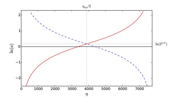
Figure 1: Evolution (red solid curve) of the natural logarithm of the scale factor as a function of conformal time in a spatially-flat, radiation-filled universe with $\Lambda$ given by recent estimates ($\Omega_{\Lambda}=0.7$ and $H_{0}=72{\rm\,km\,s^{-1}}{\rm\,Mpc^{-1}}$), with the unit of time and space given by $1{\rm\,Mpc}$. As an example, we have arbitrarily taken $a_{\rm eq}=2^{1/4}$. The blue dashed curve is the red curve reflected left-right about $\eta=\eta_{\rm tot}/2$. These curves are symmetrical not just left-right, but top-bottom if the line of reflection is taken through the value of $a$ at the mid-point, i.e. where $a=2^{1/4}$. We can thus put the curves on top of one another if we use the reciprocal, $\tilde{a}=a_{\rm eq}^{2}/a=\sqrt{2}/a$. Then the blue curve is flipped and slid up by an appropriate amount to lie on top of the red curve.

Thus any radiation-filled, flat-$\Lambda$ universe has the same basic symmetry: the development of the scale factor after the mid-point in conformal time evolution is the reciprocal (up to an overall multiplicative constant) of the development up to the mid-point.

3 Inclusion of matter and curvature

We have just shown that for radiation-only universe with $\Lambda$ the future conformal singularity is approached in a manner identical as a function of $1/a$ to the way the big bang is exited as a function of $a$. This symmetry is clearly interesting in connection with attempts, such as the CCC model, to relate the final singularity in conformal time to the big bang. The key question remaining is whether the symmetry can survive the inclusion of matter and curvature. As we now show, this is indeed the case, but only provided a suitable amount of the component labelled “missing matter” in Table 1 is present.

Making the change of variable $d\eta=dt/a$ in the Friedmann equation (1.1) and adopting the canonical equation-of-state parameters listed in Table 1, including an additional missing matter component $X$, one obtains

$$\frac{1}{H_{0}^{2}}\left(\frac{da}{d\eta}\right)^{2}=\Omega_{{\rm r},0}+\Omega_{{\rm m},0}a+\Omega_{k,0}a^{2}+\Omega_{X,0}a^{3}+\Omega_{\Lambda,0}a^{4},$$ (3.1)

where we note that the right-hand side is simply a fourth-degree polynomial in $a$. Guided by our findings in Section 2 for the radiation-only, flat-$\Lambda$ case, we make the change of variable $\tilde{a}(\eta)=\alpha^{2}/a(\eta)$, where $\alpha$ is a constant. This immediately yields

$$\frac{1}{H_{0}^{2}}\!\!\left(\frac{d\tilde{a}}{d\eta}\right)^{2}\!\!\!=\alpha^{4}\Omega_{\Lambda,0}+\alpha^{2}\Omega_{X,0}\tilde{a}+\Omega_{k,0}\tilde{a}^{2}\\ +\frac{\Omega_{{\rm m},0}}{\alpha^{2}}\tilde{a}^{3}+\frac{\Omega_{{\rm r},0}}{\alpha^{4}}\tilde{a}^{4}.$$ (3.2)

We thus obtain an identical equation in the new variable, $\tilde{a}$, if the densities are related by

$$\Omega_{{\rm m},0}=\alpha^{2}\Omega_{X,0},\quad\text{and}\quad\Omega_{{\rm r},0}=\alpha^{4}\Omega_{\Lambda,0}.$$ (3.3)

Noting that the LHS of (3.1) and (3.2) are invariant under $\eta\mapsto-\eta$, and the RHS of each does not contain $\eta$ explicitly, this means that if the conditions in equation (3.3) are satisfied, and if we measure $\eta$ from the point where $\tilde{a}=a$, i.e. where $a^{2}=\alpha^{2}$, then for general $\eta$ we will have $a(\eta)a(-\eta)=\alpha^{2}$. The relevance of satisfying (3.3) is that this leads to the derivatives of $a$ and $\tilde{a}$ matching at point when $\tilde{a}=a$, which is of course necessary if the function is to go smoothly through this point, whilst at the same time tracing out the reciprocal behaviour. We note this behaviour will be obtained even with curvature included, since the the symmetry does not require any special value of $\Omega_{k,0}$.

As a concrete example of this behaviour, we show in Fig. 2

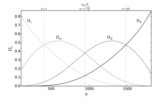
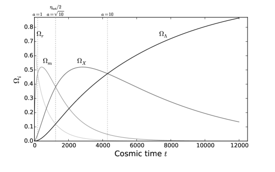
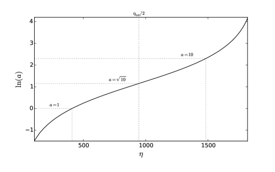
Figure 2: Evolution of a spatially-flat universe with matter and ‘missing matter’ present in the proportions discussed in the text. The top panel shows the evolution of the radiation, matter, missing matter and vacuum energy densities as a function of conformal time $\eta$, while the middle panel show the same as a function of cosmic time $t$. The bottom panel shows the evolution of the natural logarithm of the scale factor versus conformal time over the same period.

the evolution of the energy densities of the components as a function of both conformal time and cosmic time, in a spatially-flat ($\Omega_{k,0}=0$) case where equation (3.3) is satisfied, with $\alpha^{2}=10$. Specifically, in this illustrative case, we have chosen $\Omega_{{\rm m},0}=100\,\Omega_{\Lambda,0}$, $\Omega_{{\rm r},0}=100\,\Omega_{\Lambda,0}$ and $\Omega_{X,0}=10\,\Omega_{\Lambda,0}$. These particular values mean e.g. that the radiation and matter densities should be equal at $a=1$, and the ‘missing matter’ and vacuum energy densities should be equal at $a=10$, both of which can be verified easily from the bottom panel.

We see in this case that we have indeed obtained symmetry in the density parameters about the mid-point in conformal time, and moreover the $a(\eta)$ plot is again symmetric under flipping about the horizontal axis going through the value at the mid-point ($a=\sqrt{10}$), meaning that it is symmetric in the inverse scale factor in the same way as for the radiation-only case in Section 2. It is straightforward to extend this example to include curvature, which yields the same results as regards the symmetries.

It is worth noting that the form invariance of the dynamical laws governing the evolution of the conformal metric scale factor to the reciprocity transformation $\tilde{a}(\eta)=\alpha^{2}/a(\eta)$ implies an indifference of the dynamics to exchange of the roles of radiation with dark energy, and matter with ‘missing matter’, and also to exchange of the roles of the big bang and future conformal singularity. Moreover, as an intrinsic symmetry of a dynamical law, this invariance has the same status with respect to the distribution of the various contributions to the cosmological stress-energy tensor as does homogeneity and isotropy: it is only ‘broken’ by cosmological perturbations in that sense that a particular phase-space distribution of particles in the cosmological fluid may not obey it, but it remains valid in a statistical sense (either on large scales or across an ensemble of universes).

As a caveat, however, one should recall that the true equation-of-state parameters for radiation and matter (and possibly missing matter) will, in general, differ from the canonical values listed in Table 1 and vary with cosmic epoch, as discussed in the Introduction. Consequently, the RHS of (3.1) will not, in general, be a fourth-degree polynomial, in which case it no longer has the opportunity to remain form-invariant under the reciprocity transformation $\tilde{a}(\eta)=\alpha^{2}/a(\eta)$.

Nonetheless, the basic notion of symmetric behaviour at the big bang and future conformal singularity remains valid, particularly since at these extremes only massless particles are likely to be present (as argued by Penrose in the CCC model). Thus, it still seems of interest to explore the symmetry discussed here as a possible approximate symmetry of our universe. In particular, the key to realising this symmetry, is the existence of the ‘missing matter’ component, which moreover has to be present in the proportion discussed earlier, and encoded in equation (3.3). The possibility that such a ‘missing matter’ component is indeed present in our universe seems well worth testing against current cosmological observations.

4 Phenomenology

Given the motivation presented in Sections 2 and 3, we begin by investigating the phenomenology of a cosmological model containing a second component $X$ with negative pressure (in the event the energy density is positive), in addition to a cosmological constant. Since our ‘missing matter’ model (for which $w_{X}=-\frac{2}{3}$) is just a special case (albeit a very important one) of our more generic (but less theoretically well-motivated) ‘double dark energy’ model (for which $w_{X}$ is allowed to vary), we will focus here on the former as being a representative example of the latter.

In our analysis, we do not restrict the energy density $\Omega_{X}$ (at any epoch) to be positive. Although once widely accepted, the trace, strong, null, weak and dominant energy conditions all now have a somewhat weakened status following recent evidence of violations in physical systems ranging from neutron stars to inflationary cosmology, and in particular from the physics of scalar fields [14, 15]. Given this ongoing historical revision of the energy conditions, it seems appropriate to continue in the tradition of letting the observational data take precedence over theoretical prejudice. Indeed, from a Bayesian perspective, it seems prudent not to impose a prior that assigns zero probability density to negative values of $\Omega_{X}$, since this may exclude outcomes that are implied by the data.

The effect of the additional component $X$ on the global expansion history of the universe depends only on the equation-of-state parameter $w_{X}$, whereas its effect on the evolution of perturbations will also depend on the nature of the component $X$, in particular its assumed dynamical properties. We therefore consider these two issues separately.

4.1 Background evolution

The global expansion history of the cosmological model is most conveniently represented through the distance-redshift relation. Indeed, comparing the predicted relation between the luminosity distance $d_{L}$ and redshift $z$ of an object with observations of astronomical ‘standard candles’, such as Type-Ia supernovae, has provided the most direct and convincing evidence that the expansion of the universe is accelerating.

The luminosity distance to an object at redshift $z$ is given by

$$d_{L}(z)=(1+z)\frac{S_{k}(\sqrt{|\Omega_{k,0}|}\,\chi(z))}{\sqrt{|\Omega_{k,0}|}},$$ (4.1)

where $S_{k}(x)=\sinh x$, $x$, $\sin x$ for spatial curvature parameter $k=-1$, $0$, $+1$ respectively, and the comoving radial coordinate $\chi(z)$ is determined by the expansion history:

$$\chi(z)=\int_{0}^{z}\frac{d\bar{z}}{H(\bar{z})},$$ (4.2)

where $H(z)$ is obtained from the Friedmann equation (1.1). The inclusion of the $\Omega_{X,0}$ into (1.1) thus directly affects the expansion history embodied in $H(z)$, and hence can serve either to increase or decrease the luminosity distance $d_{L}(z)$ to an object at redshift $z$. Fig. 3 illustrates this effect for a few representative values of $\Omega_{X,0}$. If $\Omega_{X,0}>0$, the apparent luminosity is increased and hence the luminosity distance is reduced compared to the standard $\Lambda$CDM model. The opposite effect occurs for $\Omega_{X,0}<0$.

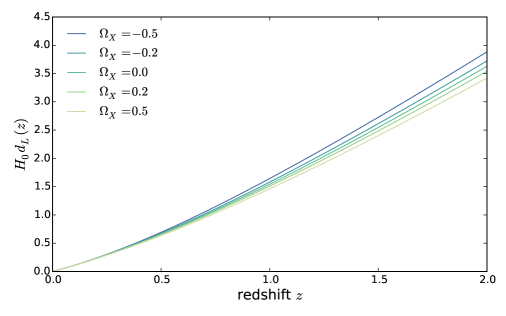
Figure 3: Dimensionless luminosity distance $H_{0}d_{L}(z)$ as a function of redshift $z$ for a concordance $\Lambda$CDM cosmology with an additional component $X$ with equation-of-state parameter $w_{X}=-\frac{2}{3}$, for different values of $\Omega_{X,0}$ (and adjusted $\Omega_{\Lambda,0}$).

The power of the luminosity distance as a cosmological probe resides in the fact that it can be simply related to apparent brightness $m(z)$ obtained directly from a set of standard candles, each (assumed to be) of absolute magnitude $M$, namely

$$m(z)=M+5\log_{10}\left[\frac{d_{L}(z)}{\rm Mpc}\right]+25,$$ (4.3)

where the constant offset ensures the usual convention that $m=M$ for an object at $d_{L}=10$ pc. Type-Ia supernovae constitute a set of ‘standardizable candles’ that can be used to constrain cosmological models in this way [16].

It should be pointed out that, for the background evolution, the combination of a cosmological constant with $w_{\Lambda}=-1$ and an additional component $X$ with constant $w_{X}$ is equivalent, under certain conditions outlined below, to a single dark energy component with a time-varying equation-of-state parameter $w_{\rm eff}(a)$ given by the ratio of the combined pressure of the two components to their combined density [11], namely

$$w_{\rm eff}(a)=\frac{-\Omega_{\Lambda,0}+w_{X}\Omega_{X,0}a^{-1}}{\Omega_{\Lambda,0}+\Omega_{X,0}\,a^{-1}}.$$ (4.4)

Examples of such models have been studied extensively [17, 18, 21, 19, 20], albeit not with the particular form of $w_{\rm eff}(a)$ given above. It is clear that the variation of $w_{\rm eff}$ with either $a$ or redshift $z$ is non-linear, so $w_{\rm eff}(a)$ is not contained within either of the common $w(z)=w_{0}+w_{1}z$ or $w(a)=w_{0}+w_{a}(1-a)$ parameterisations. More importantly, it should be noted that if $\Omega_{\Lambda,0}$ and $\Omega_{X,0}$ have different signs, as we allow in our analysis in Section 5, then $w_{\rm eff}(a)$ becomes singular at $a=|\Omega_{X,0}/\Omega_{\Lambda,0}|$. Thus, if $\Omega_{\Lambda,0}$ or $\Omega_{X,0}$ (or both) are allowed to take positive and negative values, then our missing matter (or double dark-energy) model is not, in general, described by a single time-varying dark-energy component. Nonetheless, it is worth comparing the evolution of $w_{\rm eff}$ with $a$ or $z$ implied by (4.4) with current constraints for a single time-varying dark-energy component.

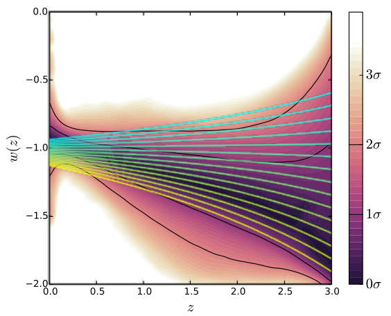
Figure 4: The evolution of $w_{\rm eff}$ in equation (4.4) with redshift $z$ (solid coloured curves) for $\Omega_{\Lambda,0}=0.8$, $\Omega_{X,0}=-0.1$, and $w_{X}$ ranging from $-1.4$ (blue line) to $0$ (yellow line) in steps of $0.1$. These curves are overlaid on a ‘free-form’ reconstruction of $w(z)$ for a single time-varying dark energy model using Planck 2015 era CMB, BAO, SNIa and Lyman-$\alpha$ data, reproduced from [22], which shows the posterior probability $\Pr(w|z)$, with colour scale in confidence interval values, and the $1\sigma$ and $2\sigma$ confidence intervals plotted as black lines.

Such a comparion is plotted in Fig. 4, where we have assumed the values $\Omega_{\Lambda,0}=0.8$, $\Omega_{X,0}=-0.1$ in (4.4), which are consistent with those obtained in Section 6 from our analysis of observational data, and $w_{X}$ ranges from $-1.4$ (blue line) to $0$ (yellow line) in steps of $0.1$. It is clear that the resulting $w_{\rm eff}(z)$ curves are indeed consistent with the constraints on $w(z)$ for a single time-varying dark energy model. For the assumed values of $\Omega_{\Lambda,0}$ and $\Omega_{X,0}$, it is worth noting that $w_{\rm eff}$ in (4.4) becomes singular at $a=1/8$, or equivalently $z=7$, and hence corresponds closely to a single time-varying dark energy model over the range of redshifts for which observational constraints are available.

4.2 Evolution of perturbations

An additional component $X$ will affect the growth of perturbations through its contribution to $H(z)$ and the evolution of the matter density. Moreover, we assume here that $X$ has the same dynamical behaviour as that usually assumed for a generic dark energy component. In particular, we use the CAMB [23] dark-energy module developed by [24], in which dark energy is assumed itself to exhibit Gaussian adiabatic perturbations. It is worth noting that, as the equation-of-state parameter approaches $-1$, the effects of the dark energy perturbations disappear, as one would expect for a pure cosmological constant. We modified the CAMB software to include our additional component and calculate the predicted power spectra of cosmic microwave background (CMB) anisotropies and matter perturbations, for several values of $\Omega_{\rm X,0}$; the values of the remaining cosmological parameters were set to their standard concordance values with $\Omega_{\Lambda,0}$ varying accordingly to ensure that $\sum_{i{=}r,m,k,X,\Lambda}\Omega_{i}=1$.

We plot the CMB power spectra in Fig. 5, from which we see that, as one might expect, the main effect of a non-zero $\Omega_{\rm X,0}$ is to shift the positions of the acoustic peaks, which are sensitive to the spatial geometry of the universe, and hence depend on the total energy density of all the components. Thus, one would expect constraints on $\Omega_{\rm X,0}$ from CMB observations to be tightly correlated with the constraints on $\Omega_{\Lambda}$ and $\Omega_{k}$. For positive values of $\Omega_{\rm X,0}$, we also see an enhancement of power on the largest scales from the late-time ISW effect. The CMB power spectrum is now well-constrained by observations over a wide range of scales.

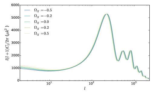
Figure 5: CMB power spectra for a concordance $\Lambda$CDM model with an additional component $X$, with equation-of-state parameter $w_{X}=-\frac{2}{3}$, for several values of $\Omega_{X,0}$.

In Fig. 6, we plot the predicted matter power spectra for different values of $\Omega_{X,0}$; again the other parameters are set to their concordance values, with $\Omega_{\Lambda,0}$ varied to incorporate the missing matter density. We see that the dominant effect of the additional component is on the normalisation of the matter power spectrum. The amplitude of fluctuations is supressed for $\Omega_{X,0}>0$ and enhanced for $\Omega_{X,0}<0$. By contrast, the positions of the acoustic oscillations, which depend on the matter density, are unaffected by the introduction of the additional component.

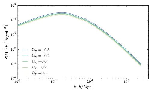
Figure 6: Matter power spectra for a concordance $\Lambda$CDM model with an additional component $X$, with equation-of-state parameter $w_{X}=-\frac{2}{3}$, for several values of $\Omega_{X,0}$.

It is worth noting that, although the background evolution of the universe is identical for our missing matter (or double dark-energy) model and for a model with a single time-varying dark energy component defined by (4.4) (provided $\Omega_{\Lambda,0}$ and $\Omega_{X,0}$ have the same sign), the evolution of perturbations is, in general, different for the two cases. This is true even in the simplest case where one assumes the same dynamical behaviour for the generic dark energy components in the two models, namely that they exhibit Gaussian adiabatic perturbations. This is illustrated in Fig. 7, in which we plot the CMB and matter power spectra for a specific example of each model.

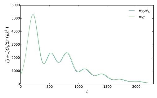
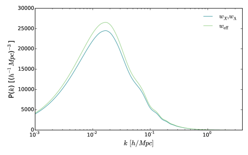
Figure 7: CMB power spectra (top) and matter power spectra (bottom) for: a concordance $\Lambda$CDM model with an additional component $X$, with equation-of-state parameter $w_{X}=-\frac{2}{3}$ and density $\Omega_{X,0}=0.2$ (dark blue line); and a CDM model with a single time-varying dark energy component with effective equation-of-state parameter $w_{\rm eff}(a)$ defined in (4.4) (light green line).

Consequently, we reiterate our earlier comment that the many previous studies of models containing a single time-varying dark-energy component are not equivalent to the study presented here.

5 Analysis

We now perform a Bayesian parameter estimation and model comparison analysis of our ‘missing matter’ and ‘double dark energy’ models, using recent cosmological observations. In particular, we use the Planck 2015 data release temperature measurements [25] and lensing data [26]. In addition to CMB data, we include distance measurements of 740 Supernovae Ia from the SNLS-SDSS collaborative effort called the joint light-curve analysis (JLA; [27]) and several Baryon Acoustic Oscillation (BAO; [28, 29, 30, 31, 32]) measurements of distance.

Throughout the analysis we consider purely Gaussian adiabatic scalar perturbations and neglect tensor contributions. We assume a modified $\Lambda$CDM model specified by the following parameters: the physical baryon density $\Omega_{\rm b}h^{2}$ and CDM density $\Omega_{\rm DM}h^{2}$, where $h$ is the dimensionless Hubble parameter such that $H_{0}=100h$ kms^-1Mpc^-1; the curvature density $\Omega_{k,0}$ of the universe; $\theta$, which is $100\times$ the ratio of the sound horizon to angular diameter distance at last scattering surface; the optical depth $\tau$ at reionisation; and the amplitude $A_{\rm s}$ and spectral index $n_{\rm s}$ of the primordial perturbation spectrum measured at the pivot scale $k_{0}=0.05$ Mpc^-1. We also include 17 nuisance parameters associated with the Planck and JLA datasets. The ranges of the uniform priors assumed on the standard $\Lambda$CDM parameters are listed in Table 2, with nuisance parameter priors set to the advised values. Our hypothetical additional component is characterised by its density parameter $\Omega_{X,0}$ and equation-of-state parameter $w_{X}$. We assume a uniform prior on $\Omega_{X,0}$ in the range $[-1,2]$ throughout. For the missing energy model, we have $w_{X}=-\frac{2}{3}$, and for the double dark energy model we assume the uniform prior $w_{X}=[-\frac{3}{2},-\frac{1}{2}]$.

To carry out the exploration of the parameter space, we first incorporate the extra component into the standard cosmological equations, by performing the minor modifications to the CAMB code [23] described in Section 4.2 (which implement a parameterised post-Friedmann (PPF) prescription for the dark energy perturbations [24]). We then include into the CosmoMC software [33] a fully-parallelised version of the nested sampling algorithm PolyChord [34, 35], which significantly increases the efficiency of calculating the Bayesian evidence and also reliably produces posterior samples even from distributions with multiple modes and/or high dimensionality. A suitable guideline for making qualitative conclusions has been laid out by Jeffreys [36]: if $\mathcal{B}_{ij}<1$ model $i$ should not be favoured over model $j$, $1<\mathcal{B}_{ij}<2.5$ constitutes significant evidence, $2.5<\mathcal{B}_{ij}<5$ is strong evidence, while $\mathcal{B}_{ij}>5$ would be considered decisive.

Parameter	Prior range
$\Omega_{\rm b,0}h^{2}$	$[0.019,0.025]$
$\Omega_{\rm dm,0}h^{2}$	$[0.095,0.145]$
$\Omega_{k,0}$	$[-0.05,0.05]$
$\theta$	$[1.03,1.05]$
$\tau$	$[0.01,0.4]$
$n_{\rm s}$	$[0.9,1.1]$
$\ln[10^{10}A_{\rm s}]$	$[2.7,4.0]$

Table 2: Ranges of the uniform priors assumed on the standard $\Lambda$CDM parameters in the Bayesian analysis.

6 Results

For comparison purposes, we first assume no additional component $X$, in order to determine the constraints imposed by the current combined data sets on the standard $\Lambda$CDM model. In particular, we find the data indicate the dominance of dark energy in the form of a cosmological constant with $\Omega_{\Lambda,0}=0.696\pm 0.007$, followed by matter density (dark matter+ baryons) $\Omega_{\rm m,0}=0.305\pm 0.007$ , and an almost negligible spatial curvature $\Omega_{k,0}=-0.0013\pm 0.0024$. We also obtain the present Hubble parameter $H_{0}=67.78\pm 0.70$. The constraints on the other parameters {$\theta,\tau,A_{\rm s},n_{\rm s}$} remain essentially unaffected by the introduction below of our additional component $X$, and so we do not consider them further.

6.1 Missing matter model

The inclusion of a missing matter component $X$ with $w_{X}=-\frac{2}{3}$ considerably broadens the parameter constraints. In particular, we find: $\Omega_{\Lambda,0}=0.734\pm 0.083$, which constitutes an order-of-magnitude increase in the error bars as compared with the standard $\Lambda$CDM model, $\Omega_{\rm m,0}=0.302\pm 0.010$, $\Omega_{k,0}=-0.0023\pm 0.0029$ and $H_{0}=68.10\pm 1.04$. Figure 8 shows 1D and 2D marginalised posterior distributions for the density parameters (note that $\Omega_{\textrm{m},0}=1-\Omega_{\Lambda,0}-\Omega_{k,0}-\Omega_{X,0}$). As expected, we observe a clear degeneracy between $\Omega_{X,0}$ and $\Omega_{\Lambda,0}$, and slight degeneracy between $\Omega_{X,0}$ and $\Omega_{k,0}$. The 1D constraint on the density parameter of missing matter is $\Omega_{X,0}=-0.034\pm 0.075$. The current data prefer a slightly negative value, which is difficult to interpret physically, but the errors suggest this not to be a significant favouring. The 1D marginal shows moderate relative probability even for $\Omega_{X,0}\sim 0.1$, and so the presence of an appreciable missing matter component cannot be ruled out. Our results are, however, still consistent with a standard $\Lambda$CDM model.

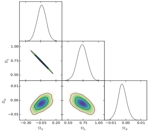
Figure 8: 1D and 2D marginalised posterior distributions for density parameters in the missing matter model (note that $\Omega_{\textrm{m},0}=1-\Omega_{\Lambda,0}-\Omega_{k,0}-\Omega_{X,0}$). The 2D constraints are plotted with $1\sigma$ and $2\sigma$ confidence contours and the cubehelix colour map [38].

This view is supported by our Bayesian model comparison. We find that the log-evidence difference (or Bayes factor) between the missing matter model and the standard $\Lambda$CDM model is $\mathcal{B}_{\Lambda+X,\Lambda}=-1.12\pm 0.53$. According to Jeffreys guideline [36, 37], the inclusion of the missing matter component is therefore slightly disfavoured, but almost indistinguishable, from a model perspective given current cosmological data.

6.2 Double dark energy model

We now allow for the equation-of-state parameter $w_{X}$ for our additional component to be a free parameter (albeit still independent of redshift), for which we assume a uniform prior in the range $w_{X}=[-\frac{3}{2},-\frac{1}{2}]$. We thus allow for the possibility that this second dark-energy component could be a form of phantom energy with $w_{X}<-1$ [39]. It should also be pointed out, however, that this parameterisation for the additional component necessarily includes a cosmological constant as the special case $w_{X}=-1$. This therefore leads to an unavoidable degeneracy between the additional component and the cosmological constant, and this should be borme in mind when interpreting the parameter constraints derived from the cosmological data.

Figure 9 shows the resulting 1D and 2D marginalised posterior distributions for $w_{X}$ and the density parameters in the model (once again, note that $\Omega_{m,0}=1-\Omega_{\Lambda,0}-\Omega_{k,0}-\Omega_{X,0}$). At the top-right of the figure we also give a representation of the 3D posterior in the $(w_{X},\Omega_{X,0},\Omega_{\Lambda,0})$ subspace, where the colour indicates the value of $\Omega_{\Lambda,0}$.

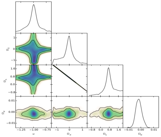
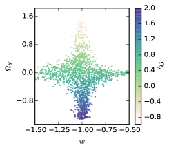
Figure 9: 1D and 2D marginalised posterior distributions for density parameters in the double dark energy model (note that $\Omega_{m,0}=1-\Omega_{\Lambda,0}-\Omega_{k,0}-\Omega_{X,0}$). The 2D constraints are plotted with $1\sigma$ and $2\sigma$ confidence contours. The top-right panel shows the 3D posterior distribution in the $(w_{X},\Omega_{X,0},\Omega_{\Lambda,0})$ subspace, where the colour code indicates the value of $\Omega_{\Lambda,0}$ using the cubehelix colour map [38].

The 1D constraints on the standard parameters are as follows: $\Omega_{\Lambda,0}=0.797\pm 0.556$, $\Omega_{\rm m,0}=0.305\pm 0.009$, $\Omega_{k,0}=-0.0015\pm 0.0024$, $H_{0}=67.86\pm 1.01$. The constraints on the parameters describing the additional second dark-energy component may be given as $w_{X}=-1.01\pm 0.16$ and $\Omega_{X,0}=-0.101\pm 0.557$, although these numbers obscure the nature of the marginal $\left(w_{X},\Omega_{X,0}\right)$-space and $\left(w_{X},\Omega_{\Lambda,0}\right)$-space distributions slightly. These results are clearly consistent with a standard $\Lambda$CDM model, although the inclusion of the additional dark-energy component has again resulted in the uncertainties in the constraints on the standard parameters being much larger than those obtained assuming a $\Lambda$CDM model. Indeed, the 1D marginal for $\Omega_{X,0}$ shows moderate relative probability even for $\Omega_{X,0}\sim\pm 0.3$, although this is likely due to a value of $w{=}-1$ simply reproducing the $\Lambda$CDM model.

Moreover, the 2D and 3D marginal distributions in Fig. 9 have interesting features that are worth noting. As might be expected, we again see a pronounced degeneracy between $\Omega_{\Lambda,0}$ and $\Omega_{X,0}$. The marginal distribution in $(\Omega_{X,0},\Omega_{\Lambda,0})$ subspace shows a strong correlation between these energy densities that would imply the potential for a trade-off between them. One might be concerned, however, that the marginal distribution plotted is strongly dominated by the contribution (after marginalising over $w_{X}$) from near $w_{X}=-1$. If so, one could then not infer the potential of a trade-off between these two energy densities at (any) other values of $w_{X}$. To investigate this possibility, we also calculated the conditional distributions in $(\Omega_{X,0},\Omega_{\Lambda,0})$ subspace for a small set of fixed $w_{X}$-values in the range $[-0.7,-1.3]$. The resulting distributions were, however, very similar to that plotted in figure 9, and so indicating that the two energy densities can indeed be traded-off against one another.

Also of interest is our Bayesian model comparison, which finds that the log-evidence difference (Bayes factor) between the double dark energy model and standard $\Lambda$CDM is $\mathcal{B}_{\Lambda+X,\Lambda}=-0.43\pm 0.45$. This shows that neither model is preferred over the other with any significance; indeed they are in the indistinguishable range of Jeffreys guideline and identical within $1\sigma$ of the error on the evidence calculation. Thus, the two additional parameters $\Omega_{X,0}$ and $w_{X}$ in the double dark energy model allow it the freedom to fit the data sufficiently better than $\Lambda$CDM to compensate for the corresponding increase in the prior volume, and hence the model is not penalised by the evidence. The Bayes factor stated is likely also aided by the broadening of posteriors on some of the parameters, as this implies a lower Occam factor associated with those parameters.

7 Discussion and Conclusions

We have investigated the possibility that there exist two dark-energy components in the universe: a cosmological constant, with $w=-1$; and an additional component $X$ with equation-of-state parameter $w_{X}$. In the first instance, we fix the equation-of-state parameter of $X$ to the value $w_{X}=-\frac{2}{3}$. Assuming the canonical values for equation-of-state parameters of the other components, this ‘missing matter’ model corresponds to the special case in which the additional component is required for the Friedmann equation written in terms of conformal time $\eta$ to be form invariant under the reciprocity transformation $\tilde{a}(\eta)=\alpha^{2}/a(\eta)$, where $\alpha^{2}$ is a constant, which is relevant to scenarios such as Penrose’s conformal cyclic cosmology (CCC) proposal. Foregoing this requirement, we then consider the more general ‘double dark energy’ model, in which $w_{X}$ is a free parameter assumed to have uniform prior in the range $w_{X}=[-\frac{3}{2},-\frac{1}{2}]$. For both models, we perform a Bayesian parameter estimation and model selection analysis, relative to standard $\Lambda$CDM, using recent cosmological observations of cosmic microwave background anisotropies, Type-Ia supernovae and large scale-structure.

For the missing matter model, the introduction of the additional component $X$ significantly broadens the constraints on the standard parameters in the $\Lambda$CDM model, but leaves their best-fit values largely unchanged. The 1D marginalised constraint on the missing matter density parameter is $\Omega_{X,0}=-0.034\pm 0.075$. Thus, current cosmological observations prefer a slightly negative value, the interpretation of which is unclear, but the posterior on this parameter is sufficiently broad that significant relative probability exits even for $\Omega_{X,0}\sim 0.1$, and so the presence of a missing matter component cannot be ruled out. To support this conclusion, our results are consistent with $\Lambda$CDM and our Bayesian model selection analysis suggests the missing matter model to be almost indistinguishable from $\Lambda$CDM, with a Bayes factor of $-1.12\pm 0.53$ log-units of evidence.

For the double dark energy model, the constraints on standard $\Lambda$CDM parameters are again considerably broadened. The 1D marginalised constraints on the vacuum and second dark energy component are $\Omega_{\Lambda,0}=0.797\pm 0.556$ and $\Omega_{X,0}=-0.101\pm 0.557$ (with $w_{X}=-1.01\pm 0.16$), respectively, which are again consistent with $\Lambda$CDM. Once more, however, the 1D marginalised posterior on $\Omega_{X,0}$ is sufficiently broad that even $\Omega_{X,0}\sim\pm 0.3$ is not ruled out. We also find that the double dark energy model has a similar Bayesian evidence to $\Lambda$CDM, and hence neither model is preferred over the other.

References

- [1] S. Perlmutter et al., Measurements of Omega and Lambda from 42 High-Redshift Supernovae, The Astrophysical Journal 517(2) (1999) 565.
- [2] A. G. Riess et al., Observational Evidence from Supernovae for an Accelerating Universe and a Cosmological Constant, The Astronomical Journal 116(3) (1998) 1009.
- [3] E. Copeland, M. Sami, and S. Tsujikawa, Dynamics of Dark Energy. International Journal of Modern Physics D 15 (2006) 1753.
- [4] R. Durrer and R. Maartens, Dark energy and dark gravity: theory overview. General Relativity and Gravitation 40 (2008) 301.
- [5] A. Vilenkin, Cosmic strings and domain walls. Physics Reports 121 (1985) 263.
- [6] R. Penrose, Cycles of Time, Bodley Head UK (2010).
- [7] R. A. Battye, M. Bucher, and D. Spergel, Domain Wall Dominated Universes, (1999) [arXiv:9908.047].
- [8] L. Conversi, A. Melchiorri, L. Mersini, and J. Silk, Are domain walls ruled out?, Astroparticle Physics 21 (2004) 443.
- [9] A. Mithani and A. Vilenkin, Did the universe have a beginning?, (2012) [arXiv:1204.4658].
- [10] R. R. Caldwell, R. Dave, and P. J. Steinhardt, Cosmological Imprint of an Energy Component with General Equation of State, Physical Review Letters, 80 (1998) 1582.
- [11] Y. Gong and X. Chen, Two-component model of dark energy, Physical Review D, 76 (2007) 123007.
- [12] M. Ibison, An Exploration of Symmetries in the Friedmann Equation, AIP Conf. Proc. 1408 (2011) 75.
- [13] R.F. Marzke and J.A. Wheeler, The geometry of space-time and the geometrodynamical standard meter, in Gravitation and Relativity, H.Y. Chiu and W.F. Hoffman, eds. (W. A. Benjamin, Inc., New York) (1964) pg. 40.
- [14] C. Barceló, M. Visser and D.V. Ahluwalia, Twilight for the Energy Conditions?, International Journal of Modern Physics D 11(10) (2002) 1553.
- [15] E. Curiel, A Primer on Energy Conditions, in Towards a Theory of Spacetime Theories, D. Lehmkuhl, G. Schiemann, and E. Scholz, eds. (Birkhäuser, New York) (2017), pg. 43.
- [16] R. Amanullah et al., Spectra and Hubble Space Telescope Light Curves of Six Type-Ia Supernovae at and the Union2 Compilation, The Astrophysical Journal 716 (2010) 712.
- [17] M. Chevallier and D. Polarski, Accelerating Universes with Scaling Dark Matter, International Journal of Modern Physics D 10(2) (2001) 213.
- [18] H. K. Jassal, J. S. Bagla, and T. Padmanabhan, WMAP constraints on low redshift evolution of dark energy, Monthly Notices of the Royal Astronomical Society 356 (2005) L11.
- [19] D. Rubin and et al., Looking Beyond Lambda with the Union Supernova Compilation, The Astrophysical Journal 695 (2009) 391.
- [20] Ö. Akarsu, T. Dereli, and J.A. Vazquez, A divergence-free parametrization for dynamical dark energy, Journal of Cosmology and Astroparticle Physics 06 (2015) 049.
- [21] I. Sendra and R. Lazkoz, SN and BAO constraints on (new) polynomial dark energy parametrizations: current results and forecasts, Monthly Notices of the Royal Astronomical Society 422 (2012) 776.
- [22] S. Hee, J.A. Vázquez, W.J. Handley, M.P. Hobson and A.N. Lasenby, Constraining the dark energy equation of state using Bayes theorem and the Kullback-Leibler divergence, Monthly Notices of the Royal Astronomical Society 466 (2017) 369.
- [23] A. Lewis, A. Challinor, and A. Lasenby, Efficient Computation of Cosmic Microwave Background Anisotropies in Closed Friedmann-Robertson-Walker Models, The Astrophysical Journal 538 (2000) 473.
- [24] W. Fang, W. Hu, and A. Lewis, Crossing the phantom divide with parametrized post-Friedmann dark energy, Physical Review D 78 (2008) 087303.
- [25] Planck Collaboration, Planck 2015 results. XI. CMB power spectra, likelihoods, and robustness of parameters, Astronomy and Astrophysics 594 (2016) A11.
- [26] Planck Collaboration, Planck 2015 results. XV. Gravitational lensing, Astronomy and Astrophysics 594 (2016) A15.
- [27] M. Betoule et al., Improved cosmological constraints from a joint analysis of the SDSS-II and SNLS supernova samples, Astronomy and Astrophysics 568 (2014) A22.
- [28] L. Anderson et al., The clustering of galaxies in the SDSS-III Baryon Oscillation Spectroscopic Survey: baryon acoustic oscillations in the Data Releases 10 and 11 Galaxy samples, Monthly Notices of the Royal Astronomical Society 441 (2014) 24.
- [29] F. Beutler et al., The 6dF Galaxy Survey: Baryon Acoustic Oscillations andthe Local Hubble Constant, Monthly Notices of the Royal Astronomical Society 416 (2011) 3017.
- [30] A. J. Ross et al., The Clustering of the SDSS DR7 Main Galaxy Sample I: A 4 per cent Distance Measure at z=0.15, Monthly Notices of the Royal Astronomical Society 449 (2015) 835.
- [31] T. Delubac et al., Baryon acoustic oscillations in the Ly forest of BOSS DR11 quasars, Astronomy and Astrophysics 574 (2015) A59.
- [32] A. Font-Ribera et al., Quasar-Lyman forest cross-correlation from BOSS DR11: Baryon Acoustic Oscillations, Journal of Cosmology and Astroparticle Physics 05 (2014) 027.
- [33] A. Lewis and S. Bridle, Cosmological parameters from CMB and other data: A Monte Carlo approach, Physical Review D 66 (2002) 103511.
- [34] W. J. Handley, M. P. Hobson and A. N. Lasenby, PolyChord: nested sampling for cosmology, Monthly Notices of the Royal Society 453 (2015) L450.
- [35] W. J. Handley, M. P. Hobson and A. N. Lasenby, PolyChord: next-generation nested sampling, Monthly Notices of the Royal Society 453 (2015) 4384.
- [36] H. Jeffreys, Theory of Probability, Oxford University Press (1998).
- [37] J. A. Vazquez, M. Bridges, M. Hobson, and A. Lasenby, Model selection applied to reconstruction of the Primordial Power Spectrum, Journal of Cosmology and Astroparticle Physics 06 (2012) 006.
- [38] D. Green, A colour scheme for the display of astronomical intensity images, Bulletin of the Astronomical Society of India 39 (2011) 289.
- [39] J. A. Vazquez, M. Bridges, M. Hobson, and A. Lasenby, Reconstruction of the Dark Energy equation of state, Journal of Cosmology and Astroparticle Physics 09 (2012) 020.