Random-matrix theory of amplifying and absorbing resonators with $\mathcal{PT}$ or $\mathcal{PTT}^{\prime}$ symmetry

Abstract

We formulate gaussian and circular random-matrix models representing a coupled system consisting of an absorbing and an amplifying resonator, which are mutually related by a generalized time-reversal symmetry. Motivated by optical realizations of such systems we consider a $\mathcal{PT}$ or a $\mathcal{PTT}^{\prime}$ time-reversal symmetry, which impose different constraints on magneto-optical effects, and then focus on five common settings. For each of these, we determine the eigenvalue distribution in the complex plane in the short-wavelength limit, which reveals that the fraction of real eigenvalues among all eigenvalues in the spectrum vanishes if all classical scales are kept fixed. Numerically, we find that the transition from real to complex eigenvalues in the various ensembles display a different dependence on the coupling strength between the two resonators. These differences can be linked to the level spacing statistics in the hermitian limit of the considered models.

1 Introduction

The investigation of nonhermitian $\mathcal{PT}$-symmetric Hamiltonians is motivated by the fact that they possess eigenvalues which are either real or occur in complex-conjugate pairs [1]. Considerable attention has been paid to the delineation of systems with a completely real spectrum, with many works focussing on exactly solvable one-dimensional situations (for reviews see [2, 3]). With the recent advent of optical implementations [4, 5] it has been realized that the appearance of complex eigenvalues drives a number of interesting switching effects [4, 5, 6, 7, 8, 9, 10, 11, 12], including the possible onset of lasing [13, 14, 15, 16], which moves the most unstable states (with energies or frequencies that have a large positive imaginary part) into the centre of attention. At the same time, these implementations motivate the study of multi-dimensional systems in which many modes become mixed by multiple scattering. Here, we investigate the formation and distribution of the complex spectrum in such situations on the basis of a statistical approach rooted in random-matrix theory [17, 18], which samples systems that respect a certain set of symmetries and share a number of well-defined characteristic energy and time scales, but differ in the microscopic details of the dynamics.

We extend earlier exploratory works of this approach [19, 20] to consider random-matrix ensembles which differ by the assumed absence or presence of elastic or dissipative magneto-optical effects. This leads to a choice between two generalized time-reversal symmetries, termed $\mathcal{PT}$ and $\mathcal{PTT}^{\prime}$ symmetry and physically motivated in [21]. These ensembles apply to a coupled-resonator geometry (with an absorbing resonator possessing $M$ internal modes coupled to a matching amplifying resonator via an interface of $N$ channels with transparency $T$, and amplification or absorption rate set to a common value $\mu$). The optical setting motivates to consider 5 particular scenarios (OO, UO, UO^′, OA and OA^′). These can be studied either based on an effective Hamiltonian or in terms on an effective time-evolution operator (a quantum map), as is described in section 2.

In section 3 we determine for each scenario the distribution of eigenvalues in the complex plane in the short-wavelength limit $M\to\infty$ at fixed $\alpha=M/N$, $T$ and $\mu$. We find that in this limit, the fraction of real eigenvalues among all eigenvalues vanishes at any finite fixed amplification and absorption rate, with the details of the eigenvalue distribution in the complex plane depending on the symmetry class. This supports the conclusion of earlier work on some of these ensembles [19] that the transition to the complex spectrum occurs at a characteristic absorption rate $\mu_{\mathrm{PT}}$ which is classically small when compared to the inverse dwell time $E_{\mathrm{T}}=1/t_{\mathrm{dwell}}=NT\Delta/2\pi$ in each part of the resonator, but large when compared to the mean level spacing $\Delta$.

In order to investigate the details of this transition we then present results of extensive numerical investigations (section 4 and 5). These reveal that the various ensembles display a different dependence of the transition on the coupling strength $T$, as well as on $M$ and $N$. This division is associated with specific mechanisms of eigenvalue coalescence, which we relate to differences in the level spacing statistics in the hermitian limit by extending the perturbative considerations of [19].

Section 6 contains our conclusions.

Throughout this work we denote eigenvalues as $E$, but set $\hbar\equiv 1$; all considerations thus directly apply to the eigenfrequencies in optical analogues of non-hermitian quantum systems.

2 Random-matrix ensembles

Following [19, 20, 21], we consider a coupled-resonator geometry where one part of the system (L) is absorbing and the other part (R) is amplifying, with the absorption and amplification rate set to a matching value $\mu$. In each part random multiple scattering at a rate $1/\tau$ results in a mixing of $M=1/\Delta\tau$ internal modes, where $\Delta$ is the mean level spacing, and the two parts are coupled together at an interface which supports $N$ open channels of transparency $T_{n}$, $n=1,2,\ldots,N$. In order to capture the consequences of multiple scattering we utilize effective Hamiltonians and quantum maps, which model these systems as illustrated in figure 1.

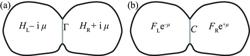
Figure 1: Illustration of (a) the effective Hamiltonian (1) and (b) the quantum map (6) used to model an absorbing resonator (L) which is symmetrically coupled (via an interface characterized by $\Gamma$ or $C$) to an amplifying resonator (R). Various symmetry classes arise depending on the constraints imposed on the internal Hamiltonians $H_{\mathrm{L}}$ and $H_{\mathrm{R}}$. The depicted situation applies to uniform amplification or absorption with rate $\mu$; further symmetry classes arise when $\mu$ is replaced by matrices $X_{\mathrm{L}}$ and $X_{\mathrm{R}}$.

2.1 Effective Hamiltonians and symmetry classes

The general structure of an effective Hamiltonian for this situation can been derived in a systematic scattering approach [19, 21]. This yields

$$\mathcal{H}=\left(\begin{array}[]{cc}H_{\mathrm{L}}-\rmi X_{\mathrm{L}}&\Gamma\\ \Gamma&H_{\mathrm{R}}+\rmi X_{\mathrm{R}}\\ \end{array}\right),$$ (1)

where the $M\times M$-dimensional hermitian matrices $H_{\mathrm{L}}$ and $H_{\mathrm{R}}$ ($X_{\mathrm{L}}$ and $X_{\mathrm{R}}$) represent the internal hermitian (anti-hermitian) dynamics in each part of the system, while the coupling matrix is of the specific form

$$\Gamma=\frac{\Delta M}{\pi}\mathrm{diag}(\underbrace{\gamma_{1},\ldots,\gamma_{N}}_{\mbox{\scriptsize$N$ entries}},\underbrace{0,\ldots,0}_{\mbox{\scriptsize$M-N$ entries}}),\quad\gamma_{n}=\frac{\sqrt{T_{n}}}{1+\sqrt{1-T_{n}}}.$$ (2)

The specific form of (1) displays a structure which goes beyond the mere symmetry requirements usually applied in mathematical classifications of nonhermitian matrices (for comprehensive overviews see [22, 23, 24]). In particular, the matrix $\Gamma$ needs to be positive definite and bounded in order to model physical coupling between two resonators. This structure resembles analogous models in mesoscopic superconductivity, where the two subspaces represent particles and holes, and the coupling is provided by Andreev reflection [25, 26, 27].

We now impose two different versions of generalized time-reversal symmetry. Traditional $\mathcal{PT}$ symmetry involves the parity operator ${\cal P}=\sigma_{x}\otimes\mathbf{1}_{M}$, where the Pauli matrix $\sigma_{x}$ interchanges the subspaces R and L, as well as the time reversal operation ${\cal T}=K$, where $K$ is the complex conjugation in a given basis, assumed to coincide with the basis of (1). Invariance under the joint $\mathcal{PT}$ operation then demands

$$\mathcal{H}={\cal P}{\cal H}^{*}{\cal P}\quad\Rightarrow\quad H_{\mathrm{L}}=H_{\mathrm{R}}^{*}=H_{\mathrm{R}}^{T},\quad X_{\mathrm{L}}=X_{\mathrm{R}}^{*}=X_{\mathrm{R}}^{T}.$$ (3)

In a $\mathcal{PT}$-symmetric basis, the secular polynomial $s(E)=\mathrm{det}\,(\mathcal{H}-E\mathbf{1}_{2M})$ has real coefficients, which constraints each eigenvalue to be real or being partnered by its complex conjugate.

In hermitian situations, the complex conjugation $\mathcal{T}$ is equivalent to taking the transpose of the matrix (thus passing from the right eigenvalue problem to the left eigenvalue problem). In non-hermitian situations, this transposition amounts to an independent operation, denoted as $\mathcal{T}^{\prime}$ [19, 21]. For a $\mathcal{PTT}^{\prime}$-symmetric situation, we now obtain the constraints

$$\mathcal{H}={\cal P}{\cal H}^{\dagger}{\cal P}\quad\Rightarrow\quad H_{\mathrm{L}}=H_{\mathrm{R}},\quad X_{\mathrm{L}}=X_{\mathrm{R}},$$ (4)

which is of interest as this yields the same spectral constraints as $\mathcal{PT}$ symmetry.

For each of these two cases, a number of ensembles can now be formulated depending on the presence or absence of additional symmetries for $H\equiv H_{\mathrm{L}}$ and $X\equiv X_{\mathrm{L}}$. In particular, we consider the cases that they may be further constrained to be real and thus symmetric (labeled O for orthogonal), complex (labeled U for unitary), or purely imaginary and thus antisymmetric (labeled A). In combination, we then arrive at 9 symmetry classes with $\mathcal{PT}$-symmetry, denoted as $S_{\mathrm{H}}S_{\mathrm{X}}$, $S_{i}=\mathrm{O},\mathrm{U},\mathrm{A}$, as well as 8 additional classes $S_{\mathrm{H}}S_{\mathrm{X}}^{\prime}$ with $\mathcal{PTT}^{\prime}$-symmetry (OO and OO^′ coincide as in this case $\mathcal{T}^{\prime}$ is an independent symmetry).

A detailed discussion of the physical requirements corresponding to the various symmetries in optical settings is given in [21]. Motivated by this context, we focus on 5 situations, OO, UO, UO^′, OA and OA^′. The most important scenario is that of OO symmetry, with $H=H^{T}=H^{*}$, $X=X^{T}=X^{*}$, which includes ordinary optical systems with gain and loss modeled by a complex refractive index. The cases of UO and UO^′ symmetry ($X=X^{T}=X^{*}$ but $H$ not further constrained) model systems with elastic magneto-optical effects, with different symmetry constraints imposed on the effective magnetic field. We will also consider the OA and OA^′ cases, as it is known that absorption can be provided by magneto-optical devices [28] (in practice, however the design of a matching magneto-optical amplification may prove challenging).

2.2 Random-matrix ensembles

The described symmetry classes are converted into statistical ensembles under convenient sampling of the $M\times M$-dimensional hermitian matrices $H$ and $X$. Specifically, depending on whether $S_{\mathrm{H}}=\mathrm{O}$ or U we choose $H$ from the standard Gaussian orthogonal or unitary ensemble (GOE or GUE) of random matrix theory [17, 18], respectively. The variance $|H_{lm}|^{2}=\sigma=1/M$ of the matrix elements is set such that the probability distribution of eigenvalues $E$ becomes stationary in the large-$M$ limit, corresponding to a Wigner semicircle law with radius 2,

$$\bar{\rho}(E)=\pi^{-1}\sqrt{1-E^{2}/4}.$$ (5)

For $S_{\mathrm{X}}=\mathrm{O}$ symmetry of the anti-hermitian part, we model uniform absorption and amplification by setting $X=\mu\mathbf{1}_{M}$. For the case $S_{\mathrm{X}}=\mathrm{A}$, we model $\rmi X=-A$ via a real antisymmetric matrix with random Gaussian elements, and quantify the degree of non-hermiticity by $\mu^{2}=M^{-1}\mathrm{tr}\overline{AA^{T}}$.

Throughout, we will model the coupling between the two parts of the system via $N\equiv\alpha M$ channels of identical transparency $T$. Together with the chosen energy scaling (5), which gives $\Delta_{0}\equiv M/\rho(E=0)=M/\pi$, the coupling matrix (2) then takes the form $\Gamma=\mathrm{diag}(\gamma,\ldots,\gamma,0,\ldots,0)=\gamma\,\mathrm{diag}(\mathbf{1}_{N},0_{M-N})$, with $N$ finite diagonal entries $\gamma=\sqrt{T}(1+\sqrt{1-T})^{-1}$.

We denote these ensembles as G$S_{\mathrm{H}}S_{\mathrm{X}}$E or G$S_{\mathrm{H}}S_{\mathrm{X}}$E^′, and specifically consider the cases GOOE, GUOE, GUOE^′, GAOE, and GAOE^′, which correspond to the optical settings described in the previous subsection.

2.3 Effective quantum maps

An alternative approach in random-matrix theory bases the considerations on circular ensembles of effective time-evolution operators [17, 18]. For the coupled-resonator geometry, the general structure of these operators has been identified in [20, 21]. They take the form of a quantum map

$${\cal F}=\sqrt{C}\left(\begin{array}[]{cc}\rme^{-\mu\tau}F_{\mathrm{L}}&0\\ 0&\rme^{\mu\tau}F_{\mathrm{R}}\\ \end{array}\right)\sqrt{C},\quad\sqrt{C}=\left(\begin{array}[]{cc}\mathrm{Re}\,\tilde{\gamma}\,P+Q&-\rmi\mathrm{Im}\,\tilde{\gamma}\,P\\ -\rmi\mathrm{Im}\,\tilde{\gamma}\,P&\mathrm{Re}\,\tilde{\gamma}\,P+Q\\ \end{array}\right),$$ (6)

which delivers quasienergies $E_{n}$ via the eigenvalue problem

$${\cal F}\psi_{n}=\lambda_{n}\psi_{n},\quad\lambda_{n}=\exp(-\rmi E_{n}\tau).$$ (7)

The properties of the interface are now encoded in the parameter $\tilde{\gamma}=\sqrt{\sqrt{R}+\rmi\sqrt{T}}$, the rank-$N$ projector $P=\mathrm{diag}(\mathbf{1}_{N},0_{M-N})$, and the complementary projector $Q=\mathbf{1}_{M}-P$. The internal dynamics are described by the $M\times M$-dimensional unitary matrices $F_{\mathrm{L}}$ and $F_{\mathrm{R}}$, which satisfy $F_{\mathrm{L}}=F_{\mathrm{R}}^{T}$ for $\mathcal{PT}$ symmetry, and $F_{\mathrm{L}}=F_{\mathrm{R}}$ for $\mathcal{PTT}^{\prime}$ symmetry. Finite $\mu$ breaks the unitarity of the quantum map. (In the specified form, (6) holds for $S_{\mathrm{X}}=\mathrm{O}$ symmetry with uniform amplification and absorption, but by the replacement $\mu\to X$ can be adapted to other symmetries.) Appropriate random-matrix ensembles follow by choosing $F=F_{\mathrm{L}}$ from the standard circular orthogonal or unitary ensembles (COE or CUE), respectively [17, 18]. We denote these circular ensembles with $\mathcal{PT}$ and $\mathcal{PTT}^{\prime}$ symmetry as C$S_{\mathrm{H}}S_{\mathrm{X}}$E and C$S_{\mathrm{H}}S_{\mathrm{X}}$E^′, respectively.

2.4 Overview of characteristic parameters and scales

In summary, each RMT ensemble is specified by the symmetry $S_{\mathrm{H}}S_{\mathrm{X}}$, as well the following 4 dimensionless parameters: the number of modes $M=1/\Delta\tau$ in each of the two parts of the system, the relative size $\alpha=N/M$ of the interface, the transparency $T$ of the interface (encoded in $\gamma$ or $\tilde{\gamma}$), and the degree of non-hermiticity $\mu/E_{\mathrm{T}}$, where $E_{\mathrm{T}}\equiv NT/2\pi\Delta$ is the Thouless parameter mentioned in the introduction. In the Hamiltonian variants of RMT, $\Delta=\pi/M$ and $E_{\mathrm{T}}=T\alpha/2$, while in the quantum map version with $\tau\equiv 1$, $\Delta=2\pi/M$ and $E_{\mathrm{T}}=T\alpha$.

3 Eigenvalue distribution in the large $M$ limit

In order to get insight into the distribution of eigenvalues in the complex plane, and the conditions under which they may accumulate on the real axis, we first consider the limit of a large number of internal modes $M\to\infty$, at fixed $\alpha=N/M$, $\mu/E_{\mathrm{T}}$ and $T$. For an optical system, this limit is realized by decreasing the wavelength (increasing the frequency) in a given resonator geometry while keeping the absorption and amplification rate $\mu$ at a wavelength-independent value. In random-matrix theory, this limit can be approached via systematic diagrammatic expansions, where the leading order captures the averaged eigenvalues density neglecting fluctuations on the scale of the level spacing [25, 29, 30, 31]. We now adapt this approach to the symmetries in question.

3.1 Generalized Pastur equation

The effective Hamiltonian ${\cal H}$ generally possesses complex eigenvalues, and the complex-analysis nature of the method employed below suggests to denote these as $z$. The distribution of eigenvalues in the complex plane can then be written as

$$\rho(z,z^{*})=\frac{1}{2M}\frac{1}{\pi}\frac{\partial{{\rm tr}\,{\cal G}_{11}}}{\partial z^{*}},$$ (8)

where ${\cal G}_{11}$ denotes the $2M\times 2M$-dimensional top-left block of the $4M\times 4M$-dimensional matrix Green function

$${\cal G}=\left(\begin{array}[]{cc}z-{\cal H}&\rmi\lambda\\ \rmi\lambda&z^{*}-{\cal H}^{\dagger}\\ \end{array}\right)^{-1}.$$ (9)

The limit $\lambda\to 0$ is implied to be taken at the end of the calculation.

In order to work out the random-matrix average we expand the matrix Green function as a geometric series

$${\cal G} = {\cal U}^{-1}\sum_{n=0}^{\infty}(-{\cal H}_{0}{\cal U}^{-1})^{n},\quad{\cal H}_{0}={\rm diag}(H,H,H,H),$$ (10)

$${\cal U} = \left(\begin{array}[]{cccc}z+\rmi\mu&-\Gamma&\rmi\lambda&0\\ -\Gamma&z-\rmi\mu&0&\rmi\lambda\\ \rmi\lambda&0&z^{*}-\rmi\mu&-\Gamma\\ 0&\rmi\lambda&-\Gamma&z^{*}+\rmi\mu\\ \end{array}\right)^{-1},$$ (15)

where the momentarily stipulated form of ${\cal H}_{0}$ holds for the GOOE and GUOE^′ ensembles (the other ensembles are discussed thereafter).

The average can now be carried out by contractions of the Gaussian random variables in $H$, which can be represented diagrammatically. The leading order (the planar limit) is given by rainbow diagrams in which the contraction lines do not cross,

$$\bar{\cal G}={\cal U}^{-1}+{\cal U}^{-1}\mathop{\mathcal{H}_{0}\bar{\cal G}\mathcal{H}_{0}}_{\raise 3.01389pt\hbox{\vrule width=0.3014pt,height=0.0pt,depth=3.01389pt}\lower 0.0pt\hbox{\vrule width=13.56248pt,height=0.0pt,depth=0.3014pt}\raise 3.01389pt\hbox{\vrule width=0.3014pt,height=0.0pt,depth=3.01389pt}}\bar{\cal G},$$ (16)

which sum up to

$$\bar{\cal G}={\cal U}^{-1}+{\cal U}^{-1}[G\otimes\mathbf{1}_{M}]\bar{\cal G}\Rightarrow\bar{\cal G}=({\cal U}^{-1}-G\otimes\mathbf{1}_{M})^{-1},$$ (17)

where $G=\frac{1}{M}{\rm tr}_{M}\,\bar{\cal G}$ is a reduced $4\times 4$ matrix Green function.

The matrix ${\cal U}^{-1}-G\otimes\mathbf{1}_{M}$ on the right-hand side of (17) separates into $N$ blocks of the form $(u_{\gamma}-G)$ and $M-N$ blocks of the form $(u_{0}-G)$, where

$$u_{\gamma}=\left(\begin{array}[]{cccc}z+\rmi\mu&-\gamma&\rmi\lambda&0\\ -\gamma&z-\rmi\mu&0&\rmi\lambda\\ \rmi\lambda&0&z^{*}-\rmi\mu&-\gamma\\ 0&\rmi\lambda&-\gamma&z^{*}+\rmi\mu\\ \end{array}\right).$$ (18)

We thus can invert each block separately, and take the partial trace on both sides. This leads to the generalized Pastur equation

$$G=\alpha(u_{\gamma}-G)^{-1}+(1-\alpha)(u_{0}-G)^{-1}$$ (19)

for the GOOE and GUOE^′ ensembles.

For the GUOE ensemble, (15) holds with ${\cal H}_{0}={\rm diag}(H,H^{*},H,H^{*})={\rm diag}(H,H^{T},H,H^{T})$. The transpositions reduce the number of rainbow diagrams in the Gaussian average, which leads to the modified equation

$$G=\alpha(u_{\gamma}-P_{1}GP_{1}-P_{2}GP_{2})^{-1}+(1-\alpha)(u_{0}-P_{1}GP_{1}-P_{2}GP_{2})^{-1},$$ (20)

where $P_{1}={\rm diag}\,(1,0,1,0)$ and $P_{2}={\rm diag}\,(0,1,0,1)$.

For the GOAE ensemble, the random matrix $A$ has to be incorporated into ${\cal H}_{0}={\rm diag}(H+A,H+A,H-A,H-A)$, while $\mathcal{U}$ is replaced by $\tilde{\mathcal{U}}=\mathcal{U}|_{\mu=0}$. Instead, $\mu$ appears via the contractions of $A$. This leads to the condition

$$G=\alpha(\tilde{u}_{\gamma}-G+RGR)^{-1}+(1-\alpha)(\tilde{u}_{0}-G+RGR)^{-1},$$ (21)

where $R=\mu\,\mathrm{diag}(1,1,-1,-1)$ and $\tilde{u}_{\gamma}=u_{\gamma}|_{\mu=0}$.

Finally, in the GOAE^′ ensemble we have ${\cal H}_{0}={\rm diag}(H+A,H-A,H-A,H+A)$, and

$$G=\alpha(\tilde{u}_{\gamma}-G+R^{\prime}GR^{\prime})^{-1}+(1-\alpha)(\tilde{u}_{0}-G+R^{\prime}GR^{\prime})^{-1},$$ (22)

where $R^{\prime}=\mu\,\mathrm{diag}(1,-1,-1,1)$.

3.2 Solution of the generalized Pastur equation

The condition (19) can be rephrased as

$$(u_{\gamma}-G)G(u_{0}-G)=u_{(1-\alpha)\gamma}-G,$$ (23)

thus, a third-degree matrix polynomial, and the versions (20)–(22) can be rewritten analogously. If we write $G$ in terms of its 16 components and eliminate these successively, we end up with a polynomial of a very large degree, which prohibits an exact analytical solution. Therefore, we pursue a semi-analytical approach which starts with the exact solution $G_{0}$ in the uncoupled case $\alpha=0$, where $G_{0}(u_{0}-G_{0})=\mathbf{1}_{4}$ (independently of $\gamma$). This is solved by $G_{0}=u_{0}/2+(u_{0}^{2}/4-\mathbf{1}_{4})^{1/2}$, where the square root of the matrix $K=u_{0}^{2}/4-\mathbf{1}_{4}=V{\rm diag}\,{k_{n}}V^{-1}$ is defined by diagonalization, $K^{1/2}=V{\rm diag}\,(\pm\sqrt{k_{n}})V^{-1}$, which here can be carried out explicitly as $K$ decouples into two independent $2\times 2$-dimensional blocks. The correct branch is determined by the limit $G_{0}(z=z^{*}=0;\lambda=0)=-\rmi\sigma_{x}\otimes\mathbf{1}_{2}$.

To describe the following steps let us denote the desired solution of (19) as $G(z,z^{*};\alpha,\lambda)$. Now, we proceed as follows: (i) We determine $G(z_{0},z_{0}^{*};0,\lambda)=G_{0}(z_{0},z_{0}^{*};\lambda)$ for a fixed value of $z_{0}$ (e.g., $z_{0}=0$) and a finite value of $\lambda$ (concretely chosen to equal the eventual value of $\alpha$, as we expect the support of the spectrum to be of that order). (ii) For values $\alpha$ increasing in small increments from zero to the desired final value, we solve (19) numerically for $G(z,z^{*};\alpha,\lambda)$, where the initial condition is taken as the solution from the previous step. (iii) Analogously, we next decrease the value of $\lambda$ to a small value (here taken as $0.001$; keeping $\lambda$ small but finite regularizes branch cuts). The same procedure can be applied to solve (20)–(22).

In practice, we find that a reliable numerical approximation of the desired solution $G(z_{0},z_{0}^{*};\alpha,0)$ is obtained in a few (about 10) steps. We can next keep $\alpha$ and $\lambda$ fixed but vary $z$ in small steps to sample the complex $z$ plane. Furthermore, by considering $z^{*}$ as a formally independent variable we can also obtain the numerical derivatives required for the calculation of the eigenvalue probability density

$$\bar{\rho}(z,z^{*})=\frac{1}{2\pi}\frac{\partial}{\partial z^{*}}(G_{11}+G_{22}).$$ (24)

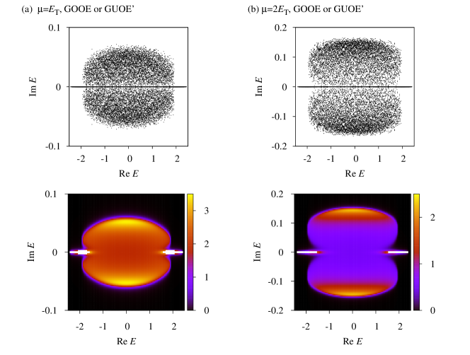
Figure 2: Eigenvalue distributions in the complex plane for the GOOE ensemble (representing an optical system without magneto-optical effects and uniform amplification or absorption), for $N/M=\alpha=0.2$, $T=1$ and (a) $\mu=0.1=E_{\mathrm{T}}$ as well as (b) $\mu=0.2=2E_{\mathrm{T}}$. The scatter plots in the top panels are obtained by numerical diagonalization of $20$ matrices $\mathcal{H}$ taken from the GOOE with $M=400$ and $N=80$. The results in the lower panels are obtained from the generalized Pastur equation (19), as described in the text. These results also apply to the GUOE^′.

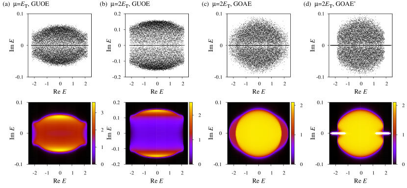
Figure 3: (a,b) Same as figure 2, but for the GUOE ensemble. (c,d) Analogous results for the GOAE and GOAE^′ ensembles, respectively, with $\mu=2E_{\mathrm{T}}$.

The lower panels in figure 2 illustrate the resulting eigenvalue distribution for the case of the GOOE and GUOE^′ ensembles, governed by (19), as density plots for $\alpha=0.2$ and $T=1$ ($\gamma=1$), for two different values of $\mu$. The top panels show the eigenvalues of $20$ random GOOE matrices with $M=400$, $N=80$. Figure 3 shows the corresponding results for the GUOE ensemble, as well as results for the GOAE and GOAE^′ ensembles for a single value of $\mu$, obtained from (20), (21) and (22), respectively. In all cases there is excellent agreement, which includes details such as the branches of the eigenvalue support extending along the real axis in the range $|\mathrm{Re}\,E|>2$, observed for the GOOE and GOAE^′ ensembles. (We also confirmed quantitative agreement by comparing histograms at fixed $\mathrm{Re}\,E$.)

The one feature which is not captured by the diagrammatic expansion is the visible accumulation of eigenvalues in the whole range $|\mathrm{Re}\,E|<2$ along the real axis. However, we find numerically that with the present scaling of parameters ($\mu/E_{\mathrm{T}}$ fixed independently of $M$), the fraction of these eigenvalues amongst all eigenvalues steadily decreases $\propto M^{-1/2}$ as $M$ increases, indicating that the real component of the spectrum indeed becomes negligible in the limit $M\to\infty$. This is consistent with the earlier prediction for the GOOE and the GOUE [19] that the transition to a complex spectrum happens for a characteristic value $\mu_{\mathrm{PT}}$ which is much less than $E_{\mathrm{T}}$ if $M$ is large. These features render the transition out of the reach of the described diagrammatic approach. In the following sections, we will first study the transition in detail based on direct numerical sampling and diagonalization of the random-matrix ensembles, and then extend the perturbative treatment of [19] to quantify the dependence of $\mu_{\mathrm{PT}}$ on $T$, $M$ and $N$.

4 Transition from a real to a complex spectrum

The transition from real to complex-conjugate pairs of eigenvalues can be quantified by considering the fraction $f_{\mathrm{c}}$ of eigenvalues which are complex; $f_{\mathrm{c}}=0$ indicates a fully real spectrum, while $f_{\mathrm{c}}=1$ if the spectrum is fully complex. We determine this fraction numerically as a function of the non-hermiticity parameter $\mu$, while keeping $T$, $M$ and $N$ fixed. In the Gaussian ensembles, the energy levels are taken only from the central region ${\rm Re}\,E\approx 0$ of the spectrum, where $\Delta_{0}\approx\pi/M$ is approximately constant. This eliminates the spectral edge effects observed in some of the eigenvalue distributions in the previous sections, and represents the typical physical conditions met in the short-wavelength limit of realistic resonators (where the effective level index is large, and the spectrum is not bounded from above). Furthermore, for $S_{\mathrm{X}}=\mathrm{O}$ (uniform absorption and amplification), we compare the results to the circular ensembles, as in these the mean level spacing is energy independent. (For $S_{\mathrm{X}}=\mathrm{A}$ the quantum maps are less convenient.)

Our eventual goal is to characterize the transition in the different ensembles by the coupling dependence of the critical scale

$$\mu_{\mathrm{PT}}=g(T)\mu_{0},$$ (25)

which we identify via $f_{\mathrm{c}}(\mu_{\mathrm{PT}})\sim 1/2$ (without requiring exact equality). The scale $\mu_{0}$ is chosen such that the function $g(T)$ does not depend on $M$ and $N$ if $M\gg N\gg 1$ (with possible exceptions for weak coupling $T<T_{\mathrm{O,A}}$, as specified below). By varying $M$ and $N$ independently we find that this scale depends on the symmetry $S_{\mathrm{X}}=\mathrm{O}$ or A, and can be suitably written as

$$\mu_{0}=\left\{\begin{array}[]{ll}\sqrt{N}\Delta/2\pi\equiv\mu_{\mathrm{O}},&\hbox{(OO, UO and UO${}^{\prime}$);}\\ \sqrt{M}\Delta/2\pi\equiv\mu_{\mathrm{A}},&\hbox{(OA, OA${}^{\prime}$).}\end{array}\right.$$ (26)

This being fixed, we set $M=200$ and $N=40$ and determine $f_{\mathrm{c}}(\mu)$ for various values of $T$ with $\mu$ measured in units of the appropriate $\mu_{0}$, as shown in figures 4–7, and focus the discussion on the ensemble-specific form of the scaling function $g(T)$ in (25).

In the GOOE and COOE (figure 4), we find that the transition becomes coupling-independent as soon as $T>T_{\mathrm{O}}$, where

$$T_{\mathrm{O}}\sim 1/N.$$ (27)

In this regime $g(T)\approx 1$; the slight $T$-dependence still observed in the plots are finite-size effects, which disappear if $M$ and $N$ are further increased. (However, in this limit $T_{\mathrm{O}}$ becomes very small, so that the behaviour for $T<T_{\mathrm{O}}$ would be difficult to illustrate; the chosen values of $M$ and $N$ thus constitute a suitable compromise.) In the GUOE and CUOE (figure 5), on the other hand, the transition displays coupling dependence throughout the whole range of $T$.

These results for OO and UO symmetry agree with the predictions in [19], which we systemize in the following section to develop a microscopic picture that also applies to the remaining ensembles considered here. The numerical results for these cases are as follows.

In the GUOE^′ and CUOE^′ (figure 6), the transition displays a similar coupling independence as in the GOOE and COOE, with $\mu_{\mathrm{PT}}$ (and thus $g(T)$) roughly scaled down by a factor of about $\sqrt{2}$.

In the GOAE and GOAE^′ (figure 7), the scale $\mu_{\mathrm{A}}$ applies. In both ensembles, there is almost no coupling dependence throughout the whole range of $T$, with exception of the weak-coupling regime $T\ll T_{\mathrm{A}}$ in the GOAE^′, which is now delineated by

$$T_{\mathrm{A}}\sim 1/N^{2}.$$ (28)

Interestingly, in this regime $g(T)$ decreases with increasing $T$, which amounts to an anomalous behaviour—the coupling between the resonators enhances the fragility of the real spectrum, in contrast to the usual situation where increasing the coupling furthers the balance of the non-hermitian effects in the system.

Note that in the limit $M=N/\alpha\to\infty$ studied in section 3, $\mu_{\mathrm{O,A}}/E_{\mathrm{T}}\to 0$ as well as $T_{\mathrm{O,A}}\to 0$.

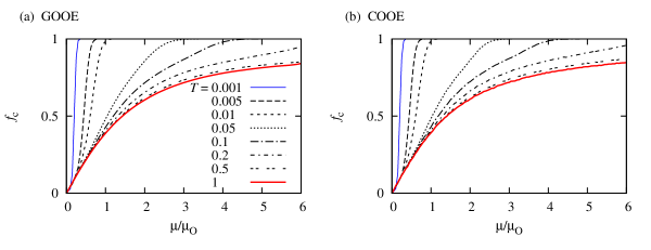
Figure 4: Average fraction $f_{\mathrm{c}}$ of complex eigenvalues as a function of the absorption rate $\mu$, scaled to $\mu_{\mathrm{O}}=\sqrt{N}\Delta/2\pi$. Panel (a) shows results for the GOOE around $\mathrm{Re}\,E=0$, while panel (b) shows results for the COOE, obtained in both cases by numerical sampling of the ensembles with $M=200$ and $N=40$. The different curves correspond to different transparencies $T$ of the interface between the amplifying and absorbing resonators. For $T>T_{\mathrm{O}}\sim 1/N$, the initial stages of the transition to a complex spectrum is coupling-independent.

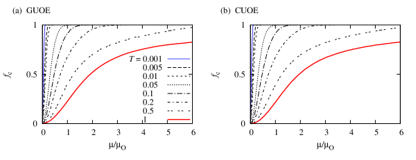
Figure 5: Same as figure 4, but for the GUOE (a) and CUOE (b). Here a clear dependence on $T$ persists throughout the entire range of this parameter.

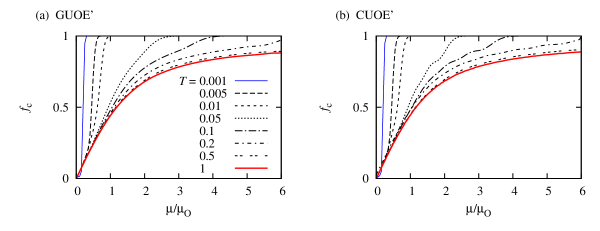
Figure 6: Same as figure 4, but for the GUOE^′ (left panel) and CUOE^′ (right panel). Again, a coupling-independent regime emerges for $T>T_{\mathrm{O}}\sim 1/N$.

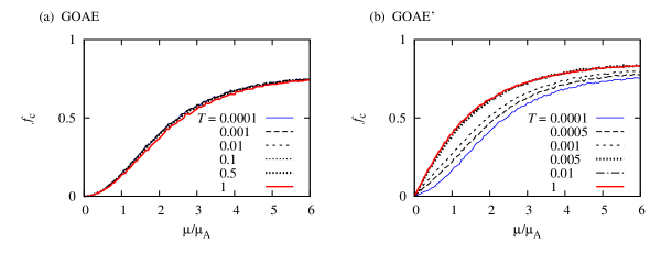
Figure 7: Same as figure 4, but for the GOAE (a) and the GOAE^′ (b), and with $\mu$ now given in units of $\mu_{\mathrm{A}}=\sqrt{M}\Delta/2\pi$. The transition is almost coupling independent, with exception of the weak-coupling regime $T<T_{\mathrm{A}}\sim 1/N^{2}$ of the GOAE^′, where the characteristic scale $\mu_{\mathrm{PT}}$ increases as $T\to 0$.

5 Relation to level spacing statistics

To explain the observations of the previous section, we now develop a microscopic picture of the transition from a real to complex spectrum. This is based on two ingredients, the level statistics in the hermitian limit $\mu=0$, and the interaction of the eigenvalues on the real axis as $\mu$ is increased. Focussing on these two ingredients is motivated by the fact that the formation of complex eigenvalues requires two real eigenvalues to coalesce. The required degree of nonhermiticity thus depends on the distance of the levels at $\mu=0$, and the typical size of the matrix elements which mix the levels. The ensembles studied here display different degrees of level repulsion and level mixing, which also depend on the coupling strength $T$, and our aim is to show that these characteristics are consistent with the coupling dependence of the complex fraction $f_{\mathrm{c}}$ reported in the previous section.

We start with some preliminary observations that justify to separate the problem of level spacing statistics at $\mu=0$ from the problem of level mixing at finite $\mu$. First, we note that at $\mu=0$, $T=0$, the system consists of two uncoupled passive resonators, which both have an identical real spectrum. In order to inspect how this degeneracy is lifted, we pass over to a $\mathcal{P}$-symmetric basis, $\mathcal{H}_{\cal P}=U\mathcal{H}U$, where $U=2^{-1/2}(\sigma_{x}+\sigma_{z})$ diagonalizes $\sigma_{x}$, which gives

$$\mathcal{H}_{\cal P}=\left(\begin{array}[]{cc}H+\Gamma&-i\mu\\ -i\mu&H-\Gamma\\ \end{array}\right)\quad\mbox{(GOOE and GUOE${}^{\prime}$)}$$ (31)

$$\mathcal{H}_{\cal P}=\left(\begin{array}[]{cc}\mathrm{Re}\,H+\Gamma&i\mathrm{Im}\,H-i\mu\\ i\mathrm{Im}\,H-i\mu&\mathrm{Re}\,H-\Gamma\\ \end{array}\right)\quad\mbox{(GUOE)}$$ (34)

$$\mathcal{H}_{\cal P}=\left(\begin{array}[]{cc}H+A+\Gamma&0\\ 0&H+A-\Gamma\\ \end{array}\right)\quad\mbox{(GOAE)}$$ (37)

$$\mathcal{H}_{\cal P}=\left(\begin{array}[]{cc}H+\Gamma&A\\ A&H-\Gamma\\ \end{array}\right)\quad\mbox{(GOAE${}^{\prime}$)}$$ (40)

In the hermitian limit $\mu=0$ (implying also $A=0$), all these transformed Hamiltonians are block diagonal, with exception of (34) for the GUOE. This is the case because in the other cases $\mathcal{P}$ is an exact symmetry; moreover, for the GOOE, GOAE, and GOAE^′, $\mathcal{T}$ and $\mathcal{T}^{\prime}$ hold separately if $\mu=0$ or $A=0$. These properties lead to different level statistics in the hermitian limit, which in all cases but for the GUOE involve the superposition of two non-interacting level sequences $E^{+}$ and $E^{-}$, obtained from $H+\Gamma$ and $H-\Gamma$, respectively. The two sequences are degenerate at $T=0$, but are modified by $\Gamma$, which perturbs the two sequences in different ways, and because of its positive definiteness also induces an approximately rigid shift.

In the non-hermitian case (finite $\mu$ or $A$) the $\mathcal{P}$ symmetry remains exact in the GOAE, while $\mathcal{T}^{\prime}$ symmetry remains exact in the GOOE and $\mathcal{T}$ symmetry remains exact in the GOAE and in the GOAE^′. These differences are reflected in the matrix elements that mix the level sequences. For this, we recall that in almost-degenerate perturbation theory, the effective Hamiltonian of two adjacent levels $E_{i}$ and $E_{j}$ is

$$\mathcal{H}_{2}=\left(\begin{array}[]{cc}E_{i}+V_{ii}&V_{ij}\\ V_{ji}&E_{j}+V_{jj}\\ \end{array}\right),$$ (41)

where $V$ is a generic perturbation. The perturbation theory is straightforward at small $T$, but as $T$ increases levels display exact or avoided crossings. One can then still base estimates by stipulating a typical spacing $\Delta$ of two adjacent levels at finite $T$, and restricting the perturbative analysis to the wavefunction overlap [19].

As a backdrop for the ensemble-dependent discussion of the details, we show in figures 8 and 9 numerically evaluated level-spacing statistics $P(s)$ at $\mu=0$, where $s$ is the distance between adjacent levels. In the Gaussian ensembles, we focus again on the bulk of the spectrum (close $\mathrm{Re}\,E\approx 0$); for $S_{\mathrm{X}}=\mathrm{O}$ these results are also compared with results from the circular ensembles (as before $M=200$ and $N=40$).

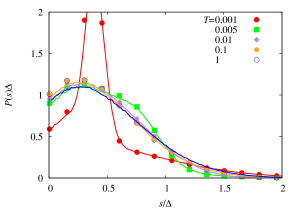
Figure 8: Level spacing distribution of real eigenvalues in the hermitian limit of the GOOE (curves) and COOE (points), obtained by numerical sampling of these ensembles with $M=200$ and $N=40$. These results also apply to the GOAE^′ and COAE^′.

In figure 8, $P(s)$ is shown for the GOOE and COOE. The data applies to the full spectrum of $\mathcal{H}$, thus, the superposition of the sequences $E^{+}$ and $E^{-}$ of $\mathcal{H}_{\mathcal{P}}$ at $\mu=0$ (with mean level spacing $\bar{s}=\Delta/2$), which is appropriate as these sequences become mixed by finite $\mu$. At small coupling $T<T_{\mathrm{O}}\sim 1/N$, the statistics is dominated by the closeness of levels which degenerate at $T=0$. Based on (41), one then finds $\mu_{\mathrm{PT}}\sim N\sqrt{T}\Delta/2\pi$, thus $g(T)\sim\sqrt{NT}\ll 1$. For $T>T_{\mathrm{O}}$, levels in the two sequences cross (giving $P(0)\approx 1/\Delta$), and the spacing statistics quickly converges to a coupling-independent form. At finite $\mu$, adjacent levels of the different sequences $E_{n}^{+}$ and $E_{m}^{-}$ with $|E_{n}^{+}-E_{m}^{-}|\sim\Delta$ are mixed by a matrix element of squared size $|\mu\langle\psi_{n}^{+}|\psi_{m}^{-}\rangle|^{2}\sim\mu^{2}/N$ [19], which becomes comparable to $\Delta^{2}$ at $\mu_{\mathrm{PT}}\sim\sqrt{N}\Delta/2\pi=\mu_{\mathrm{O}}$, up to factors of order unity because of the influence of the level fluctuations. This qualitatively explains the approximate coupling-independence of $f_{\mathrm{c}}(\mu)$, observed for this ensemble in the previous section (figure 4). One can interpolate between the weak-coupling and finite-coupling regimes by setting $g(T)\approx(1+1/NT)^{-1/2}$.

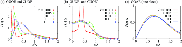
Figure 9: Same as figure 8, but for the GUOE and CUOE (left panel), the GUOE^′ and CUOE^′ (middle panel), and a single block $H+\Gamma$, corresponding to the levels that are mixed by finite $A$ in the GOAE (right panel)

The left panel of figure 9 shows the analogous result for the GUOE and CUOE. Here, finite $\Gamma$ also induces a mixing of the originally degenerate sequences $E^{+}$ and $E^{-}$, which results in a coupling-dependent level repulsion (with $P(0)=0$). This corresponds well to the persistent coupling dependence of $f_{\mathrm{c}}(\mu)$, observed in figure 5. Based on (41), one now finds $\mu_{\mathrm{PT}}\sim\sqrt{NT}\Delta/2\pi$ [19], thus $g(T)\sim\sqrt{T}$, which holds across the whole range of $T$, up to modifications of order unity, which we now can associate to the influence of the level statistics.

In the GUOE^′ and CUOE^′ (middle panel of figure 9), on the other hand, levels are again not mixed by finite $T$. Thus, a coupling-independent level statistics again emerges for $T>T_{\mathrm{O}}$, with is similar to the result for the GOOE/COOE (figure 8), with $P(0)=1/\Delta$. The modal value is shifted to slightly larger $s$, in accordance with the larger degree of level repulsion in the standard GUE/CUE [17]. This behaviour corresponds well to the approximate coupling-independence of $f_{\mathrm{c}}(\mu)$ in figure 6. We find in the perturbative treatment that $g(T)$ is the same as in the GOOE, up to a possible factor of order unity due to the small differences in the level spacing statistics.

In the GOAE, the superimposed level sequences display the same statistics as in the GOOE. However, $A$ does not mix these sequences; instead, eigenvalue coalescence must happen within a given sequence. Therefore, we consider the spacing within a fixed sequence, which is shown in the right panel of figure 9 (here the mean levels spacing is $\bar{s}=\Delta$). The result is almost indistinguishable from the standard Wigner distribution of the GOE (with $P(s)\propto s$ for small $s$) [17, 18], as the main effect of $\Gamma$ is a rigid shift; small deviations appear only for $T\approx 1$. This agrees well the corresponding behaviour of $f_{\mathrm{c}}(\mu)$ in figure 7(a). Perturbatively, the mixing is given by overlaps $a_{mn}=\langle\psi_{n}^{+}|A|\psi_{m}^{+}\rangle$ of size $\overline{a_{mn}^{2}}=\mu^{2}/M$, which must be of order $\Delta^{2}$ for eigenvalues to coalesce. Thus, we can write $\mu_{\mathrm{PT}}\approx\sqrt{M}\Delta/2\pi=\mu_{\mathrm{A}}$ (up to a factor of order unity), which is independent of $N$.

The data in figure 8 also applies to the GOAE^′, which shows a similar coupling independence, figure 7(b), as the GOOE and GUOE^′. The anomalous behaviour at small $T$ can be understood from the fact that in this regime eigenvalue coalescence predominantly occurs between levels $E_{n}^{+}$, $E_{n}^{-}$ of the two sequences that are degenerate at $T=A=0$. Thus, perturbatively their eigenvectors $\psi_{n}^{+}\approx\psi_{n}^{-}$ are identical, and the first-order coupling $\langle\psi_{n}^{-}|A|\psi_{n}^{+}\rangle=0$ because $A$ is antisymmetric (and $\psi_{n}^{\pm}$ is real). For $T>T_{\mathrm{A}}$, on the other hand, the coalescence is between originally non-degenerate levels of the two sequences, and $\mu_{\mathrm{PT}}\sim\sqrt{M}\Delta/2\pi=\mu_{\mathrm{A}}$ (up to a factor of order unity, and again independent of $N$), as in the GOAE.

6 Conclusions

In summary, motivated by recent optical realizations of non-hermitian $\mathcal{PT}$-symmetric quantum systems, we identified a number of symmetry classes which can be realized in optical resonators and differ by a choice between two generalized time reversal symmetries ($\mathcal{PT}$ or $\mathcal{PTT}^{\prime}$), as well as the absence or presence of magneto-optical effects in the hermitian and nonhermitian parts of the dynamics. Specifically we considered five scenarios, with symmetries termed OO, UO, UO^′, OA and OA^′.

Our analytical results reveal that in the short-wave limit, the fraction of real eigenvalues among all eigenvalues in the spectrum decays to zero at any classically finite amplification and absorption rate $\mu$. Based on numerical results, and an extension of the perturbative results in [19], we find that the amplification and absorption rate $\mu_{\mathrm{PT}}\approx\mu_{0}g(T)$ at which real eigenvalues turn complex is indeed characterized by a scale

$$\mu_{0}=\left\{\begin{array}[]{ll}\sqrt{N}\Delta/2\pi\equiv\mu_{\mathrm{O}},&\hbox{(OO, UO and UO${}^{\prime}$);}\\ \sqrt{M}\Delta/2\pi\equiv\mu_{\mathrm{A}},&\hbox{(OA, OA${}^{\prime}$),}\end{array}\right.$$ (42)

which is classically small but microscopically large. Furthermore, the scenarios differ in the dependence $g(T)$ on the coupling strength $T$ between the absorbing and amplifying components, which can be explained in terms of the level spacing statistics in the hermitian limit $\mu=0$, and distinct mechanisms of how these levels are then mixed when $\mu$ is finite. For UO symmetry, the transition is $T$-dependent over the whole range of this parameter. In the OO and UO^′ classes, a significant dependence is only observed for $T<T_{\mathrm{O}}\sim 1/N$, while the OA^′ symmetry class displays an anomalous dependence of the transition on the coupling strength in the range $T<T_{\mathrm{A}}\sim 1/N^{2}$. In the OA symmetry class, there is negligible coupling dependence over the whole range of $T$.

The introduced models possess a structure that respects the constraints imposed by characteristic energy and time scales, the physical nature of the amplification and absorption, and the accessible coupling strengths of a realistic (possibly semitransparent) interface. The classification of these models can be straightforwardly extended to include any symplectic, chiral, particle-hole like, or additional geometric symmetries, as previously discussed in hermitian situations [25, 26, 27, 32, 33, 34].

In this work we focussed on ensemble-specific spectral properties. However, as is generally the case in random-matrix theory, there are many quantities that are less ensemble-specific and should display a large degree of universality. The prime example is the spectral statistics of the complex eigenvalues in the bulk of the spectrum. If one is interested in such statistics, simpler models can be employed. For example, in scattering theory [31] the effective Hamiltonian has a semidefinite antihermitian part, but the bulk spectral statistics can be studied via the Ginibre ensemble with complex entries [35]. Analogously, the spectral constraints of $\mathcal{PT}$ or $\mathcal{PTT}^{\prime}$ symmetry are also obeyed by the real Ginibre ensemble, which has a much simpler matrix structure than our ensembles, and for which detailed rigorous results are available [36, 37, 38]. That this ensemble is a good model for other non-hermitian ensembles has been demonstrated, e.g., for the case of lattice QCD in [39]. Notably, in this ensemble, in the stipulated limit with fixed classical scales, the fraction of real eigenvalues decays as $1/\sqrt{M}$ [40].

An important constraint in the applicability range of any random-matrix ensemble is the requirement that many modes are well mixed by multiple scattering. This is not the case in (quasi) one dimensional $\mathcal{PT}$-symmetric disordered systems, where states are localized and the transition happens at much smaller values of $\mu$ [41, 42, 43]. Furthermore, even in wave-chaotic settings the multiple scattering can be suppressed by dynamical effects, which can lead to systematic corrections for the density of eigenvalues, as observed in [20] for the strongly amplified states in a quantum-chaotic system.

References

References

- [1] Bender, C M and Boettcher, S 1998 Real Spectra in Non-Hermitian Hamiltonians Having PT Symmetry Phys. Rev. Lett. 80, 5243–5246
- [2] Bender, C M 2007 Making sense of non-Hermitian Hamiltonians Rep. Prog. Phys. 70, 947–1018
- [3] Mostafazadeh, A 2010 Pseudo-Hermitian representation of quantum mechanics Int. J. Geom. Meth. Mod. Phys. 7, 1191–1306
- [4] Guo, A, Salamo, G J, Duchesne, D, Morandotti, R, Volatier-Ravat, M, Aimez, V, Siviloglou, G A and Christodoulides, D N 2009 Observation of PT-Symmetry Breaking in Complex Optical Potentials Phys. Rev. Lett. 103, 093902
- [5] Rüter, C E, Makris, K G, El-Ganainy, R, Christodoulides, D N, Segev, M and Kip, D 2010 Observation of parity-time symmetry in optics Nature Phys. 6, 192–195
- [6] El-Ganainy, R, Makris, K G, Christodoulides, D N and Musslimani, Z H 2007 Theory of coupled optical PT-symmetric structures Opt. Lett. 32, 2632–2634
- [7] Makris, K G, El-Ganainy, R, Christodoulides, D N and Musslimani, Z H 2008 Beam Dynamics in PT Symmetric Optical Lattices Phys. Rev. Lett. 100, 103904
- [8] Musslimani, Z H, Makris, K G, El-Ganainy, R and Christodoulides, D N 2008 Optical Solitons in PT Periodic Potentials Phys. Rev. Lett. 100, 030402
- [9] Longhi, S 2009 Bloch Oscillations in Complex Crystals with PT Symmetry Phys. Rev. Lett. 103, 123601
- [10] Ramezani, H, Kottos, T, El-Ganainy, R and Christodoulides, D N 2010 Unidirectional nonlinear PT-symmetric optical structures Phys. Rev. A 82, 043803
- [11] Longhi, S 2011 Invisibility in PT-symmetric complex crystals J. Phys. A: Math. Theor. 44, 485302
- [12] Lin, Z, Ramezani, H, Eichelkraut, T, Kottos, T, Cao, H and Christodoulides, D N 2011 Unidirectional Invisibility Induced by PT-Symmetric Periodic Structures Phys. Rev. Lett. 106, 213901
- [13] Schomerus, H 2010 Quantum Noise and Self-Sustained Radiation of PT-Symmetric Systems Phys. Rev. Lett. 104, 233601
- [14] Longhi, S 2010 PT-symmetric laser absorber Phys. Rev. A 82, 031801(R)
- [15] Chong, Y D, Ge, L and Stone, A D 2011 PT-Symmetry Breaking and Laser-Absorber Modes in Optical Scattering Systems Phys. Rev. Lett. 106, 093902
- [16] Yoo, G, Sim, H-S and Schomerus, H 2011 Quantum noise and mode nonorthogonality in non-Hermitian PT-symmetric optical resonators Phys. Rev. A 84, 063833
- [17] Mehta, M L 2004 Random Matrices, 3rd ed New York, NY: Elsevier
- [18] Haake, F 2010 Quantum signatures of chaos, 3rd ed Berlin: Springer
- [19] Schomerus, H 2011 Universal routes to spontaneous PT-symmetry breaking in non-Hermitian quantum systems Phys. Rev. A 83, 030101(R)
- [20] Birchall, C and Schomerus, H 2012 Fractal Weyl laws for amplified states in PT-symmetric resonators arXiv:1208.2259
- [21] Schomerus, H 2012 From scattering theory to complex wave dynamics in non-hermitian PT-symmetric resonators arXiv:1207.1454
- [22] Magnea, U 2008 Random matrices beyond the Cartan classification J. Phys. A: Math. Theor. 41, 045203
- [23] Akemann, G, Damgaard, P H, Osborn J C and Splittorff, K 2007 A new Chiral Two-Matrix Theory for Dirac Spectra with Imaginary Chemical Potential Nucl. Phys. B 766 34–67
- [24] Akemann, G 2011 Non-Hermitian extensions of Wishart random matrix ensembles Acta Physica Polonica B 42 901–921
- [25] Melsen, J A, Brouwer, P W, Frahm, K M and Beenakker, C W J 1996 Induced superconductivity distinguishes chaotic from integrable billiards Europhys. Lett. 35, 7.
- [26] Zirnbauer, M 1996 Riemannian symmetric superspaces and their origin in random-matrix theory J. Math. Phys. 37, 4986–5018
- [27] Altland, A and Zirnbauer, M R 1997 Nonstandard symmetry classes in mesoscopic normal-superconducting hybrid structures Phys. Rev. B 55, 1142–1161
- [28] Stoffregen, U, Stein, J, Stöckmann, H-J, Kuś, M and Haake, F 1995 Microwave Billiards with Broken Time Reversal Symmetry Phys. Rev. Lett. 74, 2666.
- [29] Janik, R A, Nowak, M A, Papp, G, Wambach, J and Zahed, I 1997 Non-Hermitian random matrix models: Free random variable approach Phys. Rev. E 55, 4100–4106
- [30] Janik, R A, Nowak, M A, Papp, G, and Zahed, I 1997 Non-hermitian random matrix models Nucl. Phys. B 501, 603–642
- [31] Fyodorov, Y V and Sommers, H-J 2003 Random matrices close to Hermitian or unitary: overview of methods and results J. Phys. A: Math. Gen. 36 3303–3347
- [32] Baranger, H U and Mello, P A 1996 Reflection symmetric ballistic microstructures: Quantum transport properties Phys. Rev. B 54, R14297
- [33] Whitney, R S, Schomerus, H and Kopp, M 2009 Semiclassical transport in nearly symmetric quantum dots. I. Symmetry breaking in the dot Phys. Rev. E 80, 056209
- [34] Whitney, R S, Schomerus, H and Kopp, M 2009 Semiclassical transport in nearly symmetric quantum dots. II. Symmetry breaking due to asymmetric leads Phys. Rev. E 80, 056210
- [35] Ginibre, J 1965 Statistical Ensembles of Complex, Quaternion, and Real Matrices J. Math. Phys. 6, 440–449
- [36] Sommers, H-J 2007 Symplectic structure of the real Ginibre ensemble J. Phys. A: Math. Theor. 40, F671–F676
- [37] Forrester, P J and Nagao, T 2007 Eigenvalue Statistics of the Real Ginibre Ensemble Phys. Rev. Lett. 99 050603
- [38] Borodin, A and Sinclair, C D, 2007 Correlation Functions of Ensembles of Asymmetric Real Matrices arXiv:0706.2670v2
- [39] Markum, H, Pullirsch, R and Wettig, T 1999 Non-Hermitian Random Matrix Theory and Lattice QCD with Chemical Potential Phys. Rev. Lett. 83, 484–487
- [40] Efetov, K B 1997 Directed Quantum Chaos Phys. Rev. Lett. 79, 491
- [41] Bendix, O, Fleishmann, R, Kottos, T and Shapiro, B 2009 Exponentially Fragile PT Symmetry in Lattices with Localized Eigenmodes Phys. Rev. Lett. 103, 030402
- [42] West, C T, Kottos, T and Prosen, T 2010 PT-Symmetric Wave Chaos Phys. Rev. Lett. 104, 054102
- [43] Scott, D D and Joglekar, Y N 2011 Degrees and signatures of broken PT symmetry in nonuniform lattices Phys. Rev. A 83, 050102(R)