Quantum Chaos and Quantum Computing Structures

Abstract

A system of quantum computing structures is introduced and proven capable of making emerge, on average, the orbits of classical bounded nonlinear maps on $\mathbb{C}$ through the iterative action of path-dependent quantum gates. The effects of emerging nonlinear dynamics and chaos upon the quantum averages of relevant observables and quantum probabilities are exemplified for a version of Chirikov’s standard map on $\mathbb{C}$. Both the individual orbits and ensemble properties are addressed so that the Poincaré map for Chirikov’s standard map, in the current quantum setting, is reinterpreted in terms of a quantum ensemble which is then formally introduced within the formalized system of quantum computing structures, in terms of quantum register machines, revealing three phases of quantum ensemble dynamics: the regular, the chaotic and an intermediate phase called complex quantum stochastic phase which shares similarities to the edge of chaos notion from classical cellular automata and classical random boolean networks’ evolutionary computation.

cgoncalves@iscsp.utl.pt

1 Quantum Chaos and Complex Systems Science

Complex quantum systems science, primarily concerned with complex quantum systems [6, 9, 10, 16, 17, 18], has grown in interdisciplinary applications to include quantum econophysics [14, 15, 19, 20], showing effective results in dealing with financial market turbulence and financial risk modelling [7, 8]. Such results open up the way for the growth of a quantum complex systems research program, which includes both complex quantum systems as well as other systems to which the quantum formalism, mathematically generalized from quantum computation theory, provides solutions that the classical formalism does not.

Given this recent growth, we can now speak of a quantum complex systems science (on purpose reversion of the first two words), that is, a branch of the complexity sciences dealing with both complex quantum systems and the generalization of the quantum formalism and methods to other areas of research dealing with complex systems in general. The current work is a contribution to such a research program, addressing emerging chaotic dynamics in qunat-based quantum computation [23].

By quantum chaos theory it is understood, here, the formal combination of quantum theory and chaos theory. Two lines of research have developed within quantum chaos theory: the first one has addressed quantum counterparts of classically chaotic systems [21], the second one has addressed chaotic quantization [1]. In the current work, we prove that qunat-based quantum computation can make emerge classical nonlinear dynamics and, in particular, chaotic orbits (section 2.). The present work is, therefore, developed from the combination of the first line of research on quantum chaos with quantum computation, showing that classically chaotic orbits can emerge from quantum computation.

In section 3., we address the example of a version of Chirikov’s standard map [4] on $\mathbb{C}$ that exemplifies chaotic dynamics emerging from quantum dynamics and the consequences for the underlying quantum system in regards to the quantum state dynamics and quantum averages.

In section 4., we address the ensemble representation and how, for a system of quantum registers, the Poincaré maps can be used as a visualization tool for emerging nonlinear dynamics in a system of $m$ quantum computing register machines. Three dynamical phases are identified in the ensemble quantum dynamics one of them, called complex quantum stochastic phase, is addressed in greater detail and linked to classical complex systems science’s notion of edge of chaos.

In section 5., the main consequences of the present work for quantum mechanics and quantum complex systems science are addressed.

2 Quantum Computing Structures, Chaos and Nonlinear Dynamics

Let a qunat bosonic quantum computing structure be defined as a triple $\left(\mathcal{H},\mathcal{A},\mathcal{U}\right)$, where $\mathcal{A}$ is an operator structure comprised of the bosonic creation and anihilation operators $a^{\dagger}$ and $a$, respectively, along with the commutator relations $\left[a,a^{\dagger}\right]=1$, $\mathcal{H}$ is the Hilbert space spanned by the basis of the number operator’s eigenstates $\hat{N}\left|n\right\rangle=n\left|n\right\rangle$, for $n=0,1,2,...$, $\mathcal{U}$ is the family of qunat quantum gates defined as the unitary operators on $\mathcal{H}$.

Now let $\mathcal{C}\subset\mathcal{H}$ be the collection of coherent states defined as the eigenstates of the anihilation operator, that is:

$$\mathcal{C}:=\left\{a\left|c\right\rangle=c\left|c\right\rangle:c\in\mathbb{C}\right\}$$ (1)

Define $Coh$ as the mathematical category [13] whose object set is $\mathcal{C}$ and morphisms are the unitary operators in $\hom(Coh)\subset\mathcal{U}$, satisfying the condition:

$$\hom(Coh):=\left\{U(c^{\prime},c)\in\mathcal{U}:U(c^{\prime},c)\left|c\right\rangle=\left|c^{\prime}\right\rangle\right\}$$ (2)

that is, each operator in $\mathcal{U}_{Coh}$ connects two, and only two, coherent states, unitarily transforming one into the other. Given the definition of $\hom(Coh)$ it immediately follows that any $U(c^{\prime},c)$ decomposes as the product of two optical displacement operators [6]: $U(c^{\prime},c)=D(c^{\prime})D(c)^{\dagger}$ (with $D(h):=\exp\left(ha^{\dagger}-h^{*}a\right)$). Defining composition operation as the product between the two unitary operators $U\left(c^{\prime\prime},c^{\prime}\right)\circ U\left(c^{\prime},c\right)=U\left(c^{\prime\prime},c^{\prime}\right)U\left(c^{\prime},c\right)$ it immediately follows, from the relation to the optical displacement operators, that the closure of $\hom(Coh)$ with respect to compostion and the associativity can be proven to be satisfied by $\hom(Coh)$. Defining identity morphic connection by $1_{c}=U(c,c)=D(c)D(c)^{\dagger}$, it follows that all of the properties of a category are satisfied by $Coh$, which can be proved from the optical displacement operator decomposition.

Now, a quantum computing basis of $Coh$ (not to be confused with the vector basis of the Hilbert space in $\left(\mathcal{H},\mathcal{A},\mathcal{U}\right)$) is defined as a subcategory $S\subseteq Coh$. Given a quantum computing basis $S$ of $Coh$ we state that a complex-valued function $F:X\mapsto Y$, with $X,\>Y\subseteq\mathbb{C}$, emerges from $S$ if, and only if, the following three conditions are met:

1. $X_{Q}\cup Y_{Q}\subseteq S$, for $X_{Q}:=\left\{\left|c\right\rangle\in\mathcal{C}:c\in X\right\}$, $Y_{Q}:=\left\{\left|c\right\rangle\in\mathcal{C}:c\in Y\right\}$, that is, the collection of coherent states corresponding to the elements of the domain of $F$ and the collection of coherent states corresponding to the elements of the codomain of $F$ are both in $S$;

2. There is a $\hom\left(S_{F}\right)\subseteq\hom\left(S\right)$ such that, for every $\left|c\right\rangle\in X_{Q}$, there is one, and only one, $U\left(c^{\prime},c\right)\in\hom\left(S_{F}\right)$ satisfying $U(c^{\prime},c)\left|c\right\rangle\in Y_{Q}$ and it is such that $c^{\prime}=F(c)$, that is, we can find a subcollection of morphisms which maps each coherent state $\left|c\right\rangle$ in $X_{Q}$ to one, and only one, coherent state in $Y_{Q}$, and this coherent state is the state corresponding to the complex number that is the image of $c$ in $Y$ under $F$.

We call the structure $Q_{F}:=\left(X_{Q}\cup Y_{Q},\hom\left(S_{F}\right)\right)$ the quantum generator of $F$ in $S$. The generator’s quantum computational pattern enacts a mathematical function through the unitary gate actions upon $X_{Q}$. Varela’s notion of enaction is the systemically proper notion to use in this case [22], quantum computation is about a systemic concrete, it takes place with systemic effects in the system’s quantum state, and, in this case, the function is not computed as an direct output of a quantum gate, it emerges out of the pattern of quantum gates and computations performed by a computing system, which leads to the notion of emergence of a function out of the quantum computation performed by a quantum computing basis, by taking the average of the anihilation operator, that is, we have the following matching between (a concrete) quantum computation and (an abstract) complex-valued function:

$$\begin{array}[]{ccc}\left|c\right\rangle\in X_{Q}&\overset{U(c^{\prime},c)}{\longrightarrow}&\left|c^{\prime}\right\rangle\in Y_{Q}\\ \downarrow&&\downarrow\\ \left\langle c|a|c\right\rangle=c\in X&\underset{F}{\longrightarrow}&\left\langle c^{\prime}|a|c^{\prime}\right\rangle=F(c)\in Y\end{array}$$ (3)

Thus, given the input $\left|c\right\rangle$ the quantum generator $Q_{F}$ unitarily transforms it in the output $\left|c^{\prime}\right\rangle=\left|F(c)\right\rangle$, this means that, evaluating, at the input, the quantum average of the anihiliation operator, we obtain $\left\langle c|a|c\right\rangle$ which coincides with $c$ because we are dealing with coherent states, on the other hand, and since we are dealing with coherent states, we obtain $\left\langle c^{\prime}|a|c^{\prime}\right\rangle=c^{\prime}$, the emergence of $F$ from the quantum computation implies, then, that $c^{\prime}=F(c)$.

In systemic terms, we are dealing with an emergence because the function is not the directing agent, indeed, this is not a top-down process, the quantum computation leads to a relation that can be synthesized by the function as identifiable in the relation between input $\left\langle c|a|c\right\rangle$ and output $\left\langle c^{\prime}|a|c^{\prime}\right\rangle$, for each $c$ in the domain of $F$, thus, the complex-valued function $F$ emerges from the quantum computation.

Theorem.

(Quantum Emergence of Complex-Valued Functions) Any complex-valued function $F:X\mapsto Y$, with $X,\>Y\subseteq\mathbb{C}$, can emerge from a quantum computing basis of $Coh$.

Proof.

From conditions (1) and (2), and from the definition of $Coh$, it follows that there is a one-to-one and onto correspondence between $\mathcal{C}$ (the collection of objects of $Coh$) and the complex numbers $\mathbb{C}$, this correspondence, defined as $\tau:\mathcal{C}\mapsto\mathbb{C}$, can be built through an operation of taking the quantum average of the anihilation operator, which leads to a corresponding complex number corresponding to the coherent state, that is:

$$\tau\left(\left|c\right\rangle\right):=\left\langle c\left|a\right|c\right\rangle=c$$ (4)

Now, any complex-valued function $F:X\mapsto Y$, with $X$, $Y\subseteq\mathbb{C}$ is such that, to each element of the domain $c\in X$, it associates one, and only one element in the codomain $Y$, let, then, $S$ be a subcategory of $Coh$ satisfying $\tau^{-1}(X)\cup\tau^{-1}(Y)\subseteq S$, we know that such a subcategory exists from the correspondence between $\mathcal{C}$ and $\mathbb{C}$. Let, also, the subcollection of morphisms $\hom\left(\tau^{-1}(X)\cup\tau^{-1}(Y)\right)\subseteq\hom\left(S\right)$ be such that for each $\left|c\right\rangle\in\tau^{-1}(X)$ there is one, and only one $U\left(c^{\prime},c\right)$ for $c^{\prime}\in\tau^{-1}(Y)$ and $c^{\prime}$ is such that $c^{\prime}=F(c)$, thus, the output in $\tau^{-1}(Y)$ of each object (coherent state) in $\tau^{-1}(X)$, under the quantum gates in $\hom\left(\tau^{-1}(X)\cup\tau^{-1}(Y)\right)$ matches the function $F$, this matching is in accordance with the following square:

$$\begin{array}[]{ccc}\left|c\right\rangle&\overset{U(c^{\prime},c)}{\longrightarrow}&\left|c^{\prime}\right\rangle\\ \tau\downarrow&&\downarrow\tau\\ c&\underset{F}{\longrightarrow}&c^{\prime}\end{array}$$ (5)

so that $F$ is locally isomorphic to each quantum computation under the structure $Q_{F}:=\left(\tau^{-1}(X)\cup\tau^{-1}(Y),\hom\left(\tau^{-1}(X)\cup\tau^{-1}(Y)\right)\right)$ which is, therefore, a quantum generator of $F$. We know that such a subcategory $S$ with a structure like $Q_{F}$ exists, since the object structure $\tau^{-1}(X)\cup\tau^{-1}(Y)$ exists in $Coh$, which follows directly from the correspondence between $\mathcal{C}$ and $\mathbb{C}$, and given that, for any pair of coherent states $\left|c\right\rangle$ and $\left|c^{\prime}\right\rangle$, there is a corresponding quantum gate in $\hom\left(Coh\right)$ such that $U(c^{\prime},c)\left|c\right\rangle=\left|c^{\prime}\right\rangle$, then, it follows that the morphisms that compose $\hom\left(\tau^{-1}(X)\cup\tau^{-1}(Y)\right)$, with the structure laid out above, also exist, therefore, we find that any complex-valued function can indeed emerge from a quantum computing basis of $Coh$. ∎

This theorem has a relevant computational consequence, in the following sense: while the quantum computing structure $\left(\mathcal{H},\mathcal{A},\mathcal{U}\right)$ works with a discrete (number operator) basis with corresponding eigenvalues expressed in natural numbers, it is capable of performing a computational jump to hypercomputation, being able to quantum computationally make emerge a function on a mathematical continuum within a quantized setting of basis states.

The immediate corollary of this theorem is that:

Corollary 1.

Any bounded nonlinear map on an complex interval $\mathbb{I}\subset\mathbb{C}$, $F:\mathbb{I}\mapsto\mathbb{I}$ can emerge from a quantum computing basis of $Coh$.

Not only can a bounded nonlinear map emerge from a quantum computing basis of $Coh$, but also its iterates:

Corollary 2.

Given any bounded nonlinear map on an complex interval $\mathbb{I}\subset\mathbb{C}$, $F:\mathbb{I}\mapsto\mathbb{I}$, each of its iterates $F^{s}$, with $s=1,2,...,$ being complex-valued functions can also emerge from a quantum computing basis of $Coh$.

From these results it, then, follows that classical nonlinear maps’ dynamics can also emerge from a quantum computing basis of $Coh$, a statement that can be placed in the form of a theorem:

Theorem.

(Emergent Classical Orbits) Let $F$ be a bounded complex-valued nonlinear map on an interval $\mathbb{I}\subset\mathbb{C}$, then, each orbit of $F$ in $\mathbb{I}$ can emerge from a quantum computing basis of $Coh$.

Proof.

Let $F$ be a bounded complex-valued nonlinear map on an interval $\mathbb{I}\subset\mathbb{C}$, From the quantum emergence of complex-valued functions theorem and corollary 1. we know that there is a quantum computing basis of $Coh$ from which this map can emerge, denote such a basis by $S$, by replacing $X$ and $Y$ by $\mathbb{I}$, in the the quantum emergence of complex-valued functions theorem’s proof, we arrive at the resulting quantum generator of $F$ in $S$: $\left(\tau^{-1}\left(\mathbb{I}\right),\textrm{hom}\left(\tau^{-1}\left(\mathbb{I}\right)\right)\right)$.

Now, let an orbit of $F$ in $\mathbb{I}$ be defined by a sequence $\left\{c_{s}\right\}_{s}$, $s=0,1,2,...$, with the following iterative scheme:

$$c_{s}=F\left(c_{s-1}\right)$$ (6)

then, from the structure of $\left(\tau^{-1}\left(\mathbb{I}\right),\textrm{hom}\left(\tau^{-1}\left(\mathbb{I}\right)\right)\right)$, we know that, for each such orbit, there is a corresponding sequence of coherent states $\left\{\left|c_{s}\right\rangle\right\}_{s}$, for $s=0,1,2,...$, obeying the scheme:

$$\left|c_{s}\right\rangle=U\left(F\left(c_{s-1}\right),c_{s-1}\right)\left|c_{s-1}\right\rangle$$ (7)

Each orbit of $F$ can, then, be addressed as the result from taking the average of the anihilation operator for a sequence of coherent states which, in turn, can be placed in isomorphic correspondence with the classical orbit under $\tau\left(\left|c_{s}\right\rangle\right)=\left\langle c_{s}\right|a\left|c_{s}\right\rangle=c_{s}$, that is:

$$\left\{\left|c_{s}\right\rangle\right\}_{s}\overset{\tau}{\longrightarrow}\left\{c_{s}\right\}_{s}$$ (8)

with the local connections:

$$\begin{array}[]{ccc}\left|c_{s-1}\right\rangle&\overset{U\left(c_{s},c_{s-1}\right)}{\longrightarrow}&\left|c_{s}\right\rangle\\ \tau\downarrow&&\downarrow\tau\\ c_{s-1}&\underset{F}{\longrightarrow}&c_{s}\end{array}$$ (9)

which allows us to conclude that each orbit of $F$ can emerge from a quantum computing basis of $Coh$, emerging from the coherent state unitary tansition in the form of a sequence of quantum averages of the anihilation operator (as per definition of $\tau$). ∎

In the last theorem, it follows that we are dealing with a form of path-dependent quantum computation, in the sense that each classical orbit emerges from a specific sequence of unitary operators actions on an initial condition $\left|c_{0}\right\rangle$, a sequence that matches the iterations of the classical map from the corresponding initial condition $\tau\left(\left|c_{0}\right\rangle\right)=c_{0}$.

If a bounded complex-valued nonlinear map on an interval $\mathbb{I\subset\mathbb{C}}$ is chaotic on $\mathbb{J\subseteq\mathbb{I}},$ then, under this last theorem, it follows that the chaotic dynamics can emerge from the quantum dynamics.

To each chaotic orbit there corresponds a specific sequence of coherent states such that the chaotic orbit emerges from the coherent state unitary transition in the form of a sequence of quantum averages of the anihilation operator. In turn, the sequence of Poisson number distribution of coherent states is such that the probability for each number state becomes expressed as a nonlinear function of a chaotic orbit:

$$P_{s}(n)=\left|\left\langle n|c_{s}\right\rangle\right|^{2}=\frac{\left|c_{s}\right|^{2n}}{n!}\exp\left(-\left|c_{s}\right|^{2}\right)$$ (10)

the quantum probabilities will thus also show chaotic fluctuations as the quantum computation proceeds. Furthermore, for initial coherent states with $\left|c_{0}\right\rangle$ and $\left|c_{0}^{\prime}\right\rangle$, whose corresponding anihilation operator eigenvalues are in a small neighborhood of each other, the resulting state sequences will diverge, with respect to their corresponding anihilation operator’s eigenvalues, in accordance with the sensitive dependence upon initial conditions that characterizes classical chaotic dynamics, this will also leave its mark upon the probabilities, which will also differ after a few quantum computations.

The quantum average of the number operator will also be a nonlinear function of a chaotic orbit, indeed, we have:

$$\left\langle\hat{N}\right\rangle=\left|c_{s}\right|^{2}=\left|F\left(c_{s-1}\right)\right|^{2}$$ (11)

We now illustrate this type of quantum computationally emergent chaos and its consequences to the sequence of number operator averages, for a version of Chirikov’s standard map on $\mathbb{C}$.

3 Chaos and Quantum Computation - Chirikov’s Standard Map on $\mathbb{C}$

Let $S$ be a subcategory of $Coh$, and $\left\{U\left(c_{s},c_{s-1}\right)\right\}_{s}$, for $s=1,2,...,$ be a sequence of qunat gates in $\hom\left(S\right)$, such that:

$$\left|c_{s}\right\rangle=U\left(F\left(c_{s-1}\right),c_{s-1}\right)\left|c_{s-1}\right\rangle$$ (12)

and, for the polar coordinate representation $c_{s-1}=r_{s-1}e^{i\phi_{s-1}}$, $F$ has the form:

$$F\left(r_{s-1}e^{i\phi_{s-1}}\right)=r_{s}e^{i\phi_{s}}$$ (13)

$$r_{s}=r_{s-1}+K\sin\phi_{s-1}$$ (14)

$$\phi_{s}=\phi_{s-1}+r_{s}$$ (15)

both equations (14) and (15) are defined modulo $2\pi$.

Given this structure, with an initially coherent state $\left|r_{0}e^{i\phi_{0}}\right\rangle$, with $r_{0}$ and $\phi_{0}$ both ranging between $0$ and $2\pi$, the sequence of qunat gates will act on the initial input leading to a sequence of state transitions that leads to a sequence of quantum averages of the anihilation operator coinciding with an orbit of a complex-valued nonlinear map with the same functional shape as Chirikov’s standard map, introduced by Chirikov in the study of the kicked rotator [4]. There are quantum mechanical consequences of this dynamics for observables of interest, in particular, in what regards the quantum average of the number operator. Taking the expected value of the number operator the following temporal dependence is found:

$$\left\langle\hat{N}\right\rangle_{s+1}=\left|c_{s+1}\right|^{2}=r_{s+1}^{2}=r_{s}^{2}+2r_{s}K\sin\phi_{s}+K^{2}\sin^{2}\phi_{s}$$ (16)

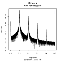
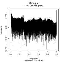
Figure 1: Spectrum estimates for $\left\langle\hat{N}\right\rangle_{s}$, from a Netlogo simulation of the system with $\left|c_{0}\right\rangle=\left|\frac{2\pi}{10}e^{i\frac{3\pi}{10}}\right\rangle$ and the following parameters: $K=0.01$ (left diagram), $K=1.4$ (right diagram). In both cases 10,000 of the first steps of the simulation were dropped, with 10,000 additional data points recorded for the case of $K=0.01$ (which was sufficient to capture the pattern), while 100,000 additional data points were recorded for the case of $K=1.4$ in order to capture more of the pattern.

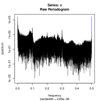
Figure 2: Spectrum estimates for $\left\langle\hat{N}\right\rangle_{s}$, from a Netlogo simulation of the system with $K=0.971635406$. The initial coherent state was set to $\left|c_{0}\right\rangle=\left|\frac{2\pi}{10}e^{i\frac{3\pi}{10}}\right\rangle$, 10,000 of the first steps of the simulation were dropped, with 100,000 additional data points recorded.

An example is shown in Fig.1, of a transition to chaotic dynamics for two different values of $K$ in terms of the power spectra for the orbits of the quantum average of the number operator for a fixed inicial condition. In the regular dynamics (Fig.1(left)) we can see several significant frequencies, marking an oscillatory behavior in the dynamics of $\left\langle\hat{N}\right\rangle_{s}$. As the parameter $K$ is increased (Fig.1(right)) the dynamics of $\left\langle\hat{N}\right\rangle_{s}$ shows the presence of stochastic behavior with a few frequency regions standing out. These frequency regions are more visible for $K$ near the critical parameter $K_{c}=0.971635406...$ above which the last KAM invariant torus is destroyed, for $K=0.971635406$, which is close to 9 decimal places of the critical parameter, the presence of a broadband spectrum of a stochastic signal shows not only a few frequency windows that stand out in the spectrum but, also, a few frequency spikes (Fig.2).

Chirikov [4] addressed such random motion in terms of the nonlinear dynamics of interactions of resonances, more specifically, the simultaneous effect on a nonlinear oscillator of several perturbations with different frequencies such that in the limiting case of very large overlapping resonant zones the system will show random motion, a process that, in the present case, due to the nonlinear path dependence of the quantum computation takes place in the sequence of phases and amplitudes of the anihilation operator’s eigenvalue orbit, leaving its markings in the number operator’s quantum averages’ sequence.

Besides the single orbit analysis, as we move on to consider the dynamics for different initial conditions, employing the Poincaré maps as visualization tools we reach, in the quantum setting, a quantum statistical description in terms of ensembles and start dealing with a complex quantum system undergoing path-dependent quantum computation making emerge different dynamical regimes with conceptual implications for the study of complex quantum systems. We, now, address this ensemble dynamics in terms of a (bosonic) quantum register machine computational structure.

4 Quantum Register Machine and Complex Quantum Systems’ Dynamics

The previous section’s results allow us to obtain a general picture of how dynamical stochasticity can emerge in the sequences of quantum averages in a quantum computation. The quantum setting, on the other hand, introduces a new perspective on the Poincaré map analysis of the classical standard map in terms of quantum statistical ensembles, which we now address.

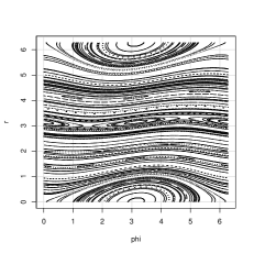
(a)

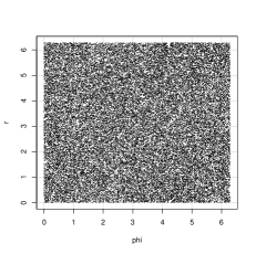
(b)

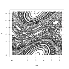
(c)

Figure 3: Quantum register machines’ dynamics with $m=120$ registers representing a coherent state ensemble simulated in Netlogo, with 400 iteration steps recorded after 10,000 initial steps, and: (a) $K=0.3$; (b) $K=7$; (c) $K=1.1$.

If one looks at the Poincaré maps of Fig.3, within the quantum setting, one may see that each of these is actually depicting the anihilation operator eigenvalue orbit for an ensemble of 120 bosonic oscillators, each undergoing a local unitary evolution, this type of parallel quantum computation, generalized to $m$-bosonic oscillators can be addressed by a $m$-entry quantum register machine, formalized from the single qunat bosonic quantum computing structures.

Indeed, given the triple $\left(\mathcal{H},\mathcal{A},\mathcal{U}\right)$, introduced in section 1., then, define the $m$-entry quantum register machine by the tensor product structure $\left(\mathcal{H}^{m},\mathcal{A}^{m},\mathcal{U}^{m}\right)=\bigotimes_{j=1}^{m}\left(\mathcal{H}_{j},\mathcal{A}_{j},\mathcal{U}_{j}\right)$, such that:

• Each $\left(\mathcal{H}_{j},\mathcal{A}_{j},\mathcal{U}_{j}\right):=\left(\mathcal{H},\mathcal{A},\mathcal{U}\right)$, that is, each triple in the tensor product is a labeled copy of a qunat bosonic quantum computing structure;

• $\mathcal{H}^{m}:=\bigotimes_{j=1}^{m}\mathcal{H}_{j}$ is a tensor-product of $m$ copies of the same Hilbert space;

• $\mathcal{A}^{m}:=\left\{a_{i}:i=1,2,...,m\right\}\cup\left\{a_{j}^{\dagger}:j=1,2,...,m\right\}$, where the creation and anihilation operators obey the bosonic commutation relations $\left[a_{i},a_{j}\right]=0$, $\left[a_{i}^{\dagger},a_{j}^{\dagger}\right]=0$ and $\left[a_{i},a_{j}^{\dagger}\right]=\delta_{i,j}$;

• $\mathcal{U}^{m}$ is the family of unitary operators on $\mathcal{H}^{m}$.

In this case, the creation and anihilation operators can act on the corresponding bosonic oscillator without affecting the rest, which is in accordance with the fact that we are dealing with ensembles that have a field-like computational behavior.

Given the above assumptions it follows that the number operators commute $\left[\hat{N}_{i},\hat{N}_{j}\right]=0$ for $i\neq j$, and the basis for the Hilbert space $\mathcal{H}^{m}$ is given by $\left\{\left|n_{1},n_{2},...,n_{m}\right\rangle:n_{j}\in\mathbb{N}_{0},j=1,2,...,m\right\}$. The registers are assumed to be sequential, much like it takes place in a Turing machine, this means that the matching of a quantum ensemble of bosonic oscillators to a register machine is unique up to a permutation of registers, the fact that one works with a particular register sequence, means that any results regarding the quantum ensemble, specifically obtained for a quantum register machine in which the labeling is irrelevant, can be generalized for all of the other permutations of registers.

Now, given a configuration of registers we can define the $\mathcal{C}_{m}\subset\mathcal{H}_{m}$ to be the collection of $m$-coherent states on $\mathcal{H}_{m}$ defined as:

$$\mathcal{C}_{m}:=\left\{\left|c(1),c(2),...,c(m)\right\rangle:c(j)\in\mathbb{C},\>j=1,2,...,m\right\}$$ (17)

that is, each register in $\mathcal{C}_{m}$ corresponds to a bosonic oscillator in a coherent state. We can, thus, define the $m$-coherent states category $Coh^{m}$ as the product category of $m$ copies of $Coh$ and such that each projection functor is labeled by the corresponding register, that is:

$$\begin{array}[]{ccccc}Coh_{i}&\overset{i}{\longleftarrow}&Coh^{m}&\overset{j}{\longrightarrow}&Coh_{j}\end{array}$$ (18)

$$Coh_{i}\overset{id_{Coh_{i}}}{\longrightarrow}Coh_{j}$$ (19)

where $id_{Coh_{i}}$ is the identify functor of $Coh_{i}$. From the (18) and (19), it follows that the product category is also indexing each copy of $Coh$ to a register, so that we have:

$$\left|c(1),c(2),...,c(m)\right\rangle\overset{j}{\longrightarrow}\left|c(j)\right\rangle$$ (20)

Since $Coh^{m}$ is a product category, the morphisms of $Coh^{m}$ must conserve the local morphic connections of each component category, that is:

$$U\left(c^{\prime}(j),c(j)\right)\left|...,c(j),...\right\rangle=\left|...,c^{\prime}(j),...\right\rangle$$ (21)

which means that the unitary change of the $j$-th coherent state to another coherent state in nothing alters the other registers’ configuration.

For the Chirikov map, we, then, have the following quantum iterative transition rule:

$$\prod_{j=1}^{m}U\left(F_{Chirikov}\left(c_{s}(j)\right),c_{s}(j)\right)\left|c_{s}(1),c_{s}(2),...,c_{s}(m)\right\rangle$$ (22)

The Poincaré map for Chirikov’s standard map becomes, in this case, a visual representation of this dynamics of each of the ensemble elements with respect to the corresponding anihilation operator eigenvalue in polar representation, thus, for chaotic orbits, even if $\left|c_{0}(1),c_{0}(2),...,c_{0}(m)\right\rangle$ begins with coherent states very close to each other, in terms of the corresponding anihilation operators’ eigenvalues, the sensitive dependence upon initial conditions will, then, lead to a divergence between the corresponding anihilation operators’ eigenvalues, for each element of the ensemble.

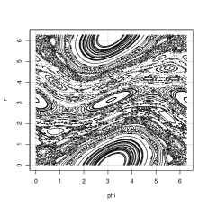
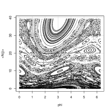
Figure 4: Complex quantum stochastic phase, for $K=0.97163541$, simulated in Netlogo, for an ensemble of size $m=120$, with 400 iteration steps recorded after 10,000 initial steps. On the left is the ensemble dynamics resulting for the quantum register machines computation, on the right is the corresponding number operator quantum average dynamics for the same simulation.

For values of $K$ sufficiently high to destroy some of the KAM tori, but not high enough, the dynamics will combine elements of regularity with randomness, becoming an exemplary picture of complexity in its interweaving of regularity and randomness (Fig.3(c), Fig.4(left)).

We can find, in the quantum register’s dynamics, a quantum computational example of the three phases of complex systems’ distributed computing dynamics, previously identified within classical approaches to evolutionary computation: a regular phase (Fig.3(a)), a chaotic phase (Fig.3(b)), and an intermediate phase (Fig.3(c), Fig.4(left)).

The chaotic phase takes hold after the $K>K_{c}$, when the last KAM invariant torus has been destroyed, thus, for $K=7$ (Fig.3(b)), we find the system in a fully chaotic phase, no regular dynamical structures present. For low $K$ the system shows a predominantly regular dynamical motion (Fig.3(a)). For $K$ above or below $K_{c}$, but neither too below nor too above, we find the system in the intermediate phase with regular and chaotic dynamics (Fig.3(b), Fig.4(left)).

The degree of dominance of chaotic elements in the quantum ensemble versus the regular elements is dependent upon the value of $K$, this intermediate phase can be called complex quantum stochastic phase, in classical complex systems science it has been called edge of chaos [5, 11, 12].

In the current case, the complex quantum stochastic phase allows one to link the notion of edge of chaos, found in classical computing examples of cellular automata [5, 12] and random boolean networks [11], to the quantum register dynamics’ phase transition to chaos, where the critical line $K_{c}$ plays the role of a reference marker around which we find the intermediate stages of the complex quantum stochastic phase.

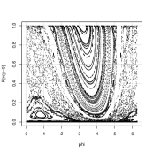
Figure 5: Ensemble ground-state quantum probabilities’ dynamics, for $K=0.979$, simulated in Netlogo, for $m=120$ quantum registers, with 400 iteration steps recorded after 10,000 initial steps.

An example of the complex quantum stochastic phase is shown in Fig.4(left), for $K$ above but very close to $K_{c}$, for an ensemble of 120 elements. The consequences of this phase for the dynamics of the quantum averages of each of the $\hat{N}_{j}$ number operators, plotted as a function of the corresponding phases $\phi_{j}$, for each register, is shown in Fig.4(right). Thus, the quantum computing, by making emerge a classical dynamics, leads to a pattern of regular dynamics, intermixed with randomness at the level of the quantum average occupation numbers of each register, leading to a basic example of complex quantum field dynamics (if the register indices are made to correspond to different quantum field modes) emerging from parallel path-dependent quantum computation. Such a complex quantum field dynamics can also be seen for the dynamics of the probabilities, for each “mode”, of finding zero particles in that “mode”, that is, the quantum probabilties $P_{s}\left[n\left(j\right)=0\right]$ dynamics for each quantum register, as shown in Fig.5 for $K=0.979$.

A striking feature, observable in Fig.5, is the fact that the quantum computation dynamics drives some of the registers (field modes) to chaotic dynamics that very nearly approach zero quanta states$\left|...,n(j)=0,...\right\rangle$ with probabilities close to $1$, which is consistent with an almost “spontaneous collapse” of the corresponding register’s quantum bosonic oscillator coherent quantum state to one of the Hilbert space basis eigenstates.

5 Conclusion

Classical chaotic dynamics is source of stochastic behavior, emergent from the nonlinear system’s deterministic dynamics, so that, even in the absence of environmental noise, the system behaves randomly, demanding a statistical description [16]. In quantum systems, chaos leads to an even greater diversity of dynamical behaviors, for instance, as addressed in [2], dissipative quantum chaos in a quantum system can lead to delocalization of wave packets induced by the instability of chaotic dynamics as well as to localization due to dissipation, the transition from localization to delocalization taking place when the dissipation time $\frac{1}{\gamma}$ ($\gamma$ being the dissipation rate) becomes larger than the Ehrenfest time $t_{E}\sim\frac{\left|\ln\hbar\right|}{\lambda}$, a similar “localization/collapse” phenomenon also takes place with respect to the ground-state energy eigenstates of bosonic oscillators, in the present article’s example, on the other hand, as addressed in [3], quantum dynamics can also suppresses chaos by conserving invariant tori that would otherwise be destroyed.

In the current work, a source of chaotic dynamics in quantum systems is addressed in terms of quantum computing structures. Sequences of quantum gates can operate upon an initial input state producing a sequence of quantum states in which both quantum probabilities as well as quantum averages fluctuate randomly and show dynamical instability as an emergent result from the system’s quantum computation, thus, unitary evolution, taking place in a path-dependent iterative way, can lead to chaotic orbits at the quantum state level, affecting both probabilities as well as quantum averages.

Dynamical stochasticity in quantum computing systems is, therefore, possible leading to dynamical instability of eigenvalues with the usual sensitive dependence upon initial conditions characterizing chaotic dynamics, to this is added the fact that quantum averages and quantum probabilities can become mathematically expressed as nonlinear functions of chaotic maps.

On the other hand, once we pass from the orbit-based picture to the ensemble picture, the Poincaré maps can become visual representations of the quantum ensemble’s state transition, leading us directly to a complex quantum systems’ approach. The field-like behavior of parallel quantum computation allows one to theoretically show that a quantum field may make emerge complex dynamics already exemplifying at that which is the most fundamental level of nature the three dynamical phases addressed in complex systems science: the regular, the chaotic and the complex in-between regime that intermixes randomness and regularity.

For complex quantum systems with chaotic dynamics, this intermixed regime, takes place as an intermixture between chaotic dynamics in the quantum states’ orbits and regular dynamics, that is, a complex intermixture between quantum dynamical stochasticity and regularity, which explains the notion of complex quantum stochastic phase.

These results, generalized by the quantum computing formalism, may help quantum econophysics address major puzzles, for both economics and finance, such as: the emergence of continuous state-like dynamics (including chaotic dynamics) in discrete (quantized) variables [8]. Quantum chaos theory is, thus, a fruitful basis for expanding both complex quantum systems science and quantum econophysics within the growing framework of a quantum complex systems science.

Figures

References

- [1] Beck, C. (2002). “Spatio-Temporal Chaos and Vacuum Fluctuations of Quantized Fields”. World Scientific, Singapore.
- [2] Carlo, G.; Benenti, G. and Shepelyansky, D.L. (2005). “Dissipative quantum chaos: transition from wave packet collapse to explosion”. Phys. Rev. Lett. 95, 164101.
- [3] Casetti, L.; Gatto, R. and Modugno, M. (1997). “Chaos in effective classical and quantum dynamics”. Phys.Rev. E57 (1998) 1223-1226.
- [4] Chirikov, B.V. ([1969], 1971). “Research Concerning the Theory of Non-linear Resonance and Stochasticity”. Report 267, Nuclear Physics Institute of the Siberian Section of the USSR Academy of Sciences, Novosibirsk. CERN Translation.
- [5] Crutchfield, J. P. and Young, K. (1990). “Computation at the Onset of Chaos”, in Entropy, Complexity, and the Physics of Information, Zurek, W. (Ed.), SFI Studies in the Sciences of Complexity, VIII, Addison-Wesley, Reading, USA, 223–269.
- [6] Gardiner, C.W. and Zoller (2004). “Quantum Noise - A Handbook of Markovian and Non-Markovian Quantum Stochastic Methods with Applications to Quantum Optics”. Springer, Germany.
- [7] Gonçalves, C.P. (2012). “Financial Turbulence, Business Cycles and Intrinsic Time in an Artificial Economy”. Algorithmic Finance (2012), 1:2, 141-156.
- [8] Gonçalves, C.P. (2012). “Chaos and Nonlinear Dynamics in a Quantum Artificial Economy”. arXiv:1202.6647v1 [nlin.CD].
- [9] Haake, F. (2010). “Quantum Signatures of Chaos”. Springer, Germany.
- [10] Haken, H. (1985). “Towards a Quantum Synergetics: Pattern Formation in Quantum Systems far from Thermal Equilibrium”. Phys. Scr. 32 274.
- [11] Kauffman, S.A. (1993). “The Origins of Order: Self-Organization and Selection in Evolution. Oxford University Press, USA.
- [12] Langton, C. (1990). “Computation at the edge of chaos”. Physica D, 42, 1990.
- [13] Mac Lane, S. (1971). “Categories for the Working Mathematician”. Springer, USA.
- [14] Piotrowski, E.W. and Sladkowski, J. (2002). “Quantum Market Games”. Physica A, 2002, Vol.312, 208-216.
- [15] Piotrowski, E.W. and Sladkowski, J. (2008). “Quantum auctions: Facts and myths”. Physica A, Vol. 387, 15, 3949-3953.
- [16] Prigogine, I. (1997). “The End of Certainty: Time, Chaos, and the New Laws of Nature”. The Free Press, USA.
- [17] Prigogine, I. (2003). “Is Future Given?”. World Scientific Publishing Co., Singapore.
- [18] Reichl, L.E., (2004). “The Transition to Chaos - Conservative Classical Systems and Quantum Manifestations”. Springer-Verlag, USA.
- [19] Saptsin, V. and Soloviev, V. (2009). “Relativistic quantum econophysics - new paradigms in complex systems modelling”. arXiv:0907.1142v1 [physics.soc-ph].
- [20] Saptsin, V. and Soloviev, V. (2011). “Heisenberg uncertainty principle and economic analogues of basic physical quantities”. arXiv:1111.5289v1 [physics.gen-ph].
- [21] Stöckmann, H.-J. (2000). “Quantum Chaos - an introduction”. Cambridge University Press, UK.
- [22] Varela, F. (1997). “Invitation aux sciences cognitives”. Seuil, France.
- [23] Zimand, M. (2004). “Computational Complexity: A Quantitative Perspective”. Elsevier. The Netherlands.