Knots in lattice homology

Abstract.

Assume that $\Gamma_{v_{0}}$ is a tree with vertex set $\mathrm{Vert}(\Gamma_{v_{0}})=\{v_{0},v_{1},\ldots,v_{n}\}$, and with an integral framing (weight) attached to each vertex except $v_{0}$. Assume furthermore that the intersection matrix of $G=\Gamma_{v_{0}}-\{v_{0}\}$ is negative definite. We define a filtration on the chain complex computing the lattice homology of $G$ and show how to use this information in computing lattice homology groups of a negative definite graph we get by attaching some framing to $v_{0}$. As a simple application we produce families of graphs which have arbitrarily many bad vertices for which the lattice homology groups are shown to be isomorphic to the corresponding Heegaard Floer homology groups.

1. Introduction

It is an eminent problem in low dimensional topology to find simple computational schemes for the recently defined invariants (e.g. Heegaard Floer and Monopole Floer homologies) of 3- and 4-manifolds. In particular, the minus-version $\rm{HF}^{-}$ of Heegaard Floer homology (defined over the polynomial ring $\mathbb{F}[U]$, where $\mathbb{F}$ denotes either $\mathbb{Z}$ or the field $\mathbb{Z}/2\mathbb{Z}$ of two elements) is of central importance. In [8] a computational scheme for the $\rm{HF}^{-}$ groups was presented, which is rather hard to implement in practice. This result was preceded by a more practical way of determining these invariants for those 3-manifolds which can be presented as boundary of a plumbing of spheres along a negative definite tree which has at most one bad vertex [21]. The idea of [21] was subsequently extended by Némethi [9], and in [10] a new invariant, lattice homology was proposed. It has been conjectured that lattice homology determines the Heegaard Floer groups when the underlying 3-manifold is given by a negative definite plumbing of spheres along a tree. Common features (eg. the existence of surgery exact triangles) have been verified for the two theories (in [19] for the Heegaard Floer setting, while in [2, 12] for lattice homology), and the existence of a spectral sequence connecting the two theories has been found [17]. For further related results see [11, 13].

In the present work we extend these similarities by introducing filtrations on lattice homologies induced by vertices, mimicking the ideas of knot Floer homologies developed in the Heegaard Floer context in [22, 26]. This information then (just as in the Heegaard Floer context) can be conveniently used to determine the lattice homology of the graph when the distinguished vertex is equipped with some framing (corresponding to the surgery formulae in Heegaard Floer theory, cf. [24]).

In more concrete terms, suppose that $\Gamma_{v_{0}}$ is a given tree (or forest), with each vertex $v$ in $\mathrm{Vert}(\Gamma_{v_{0}})-v_{0}$ equipped with a framing (or weight) $m_{v}\in\mathbb{Z}$. Let $G$ denote the tree (or forest) we get by deleting $v_{0}$ and the edges emanating from it. Suppose that $G$ is negative definite. We will define the master complex ${\mathbb{MCF}}^{\infty}(\Gamma_{v_{0}})$ of $\Gamma_{v_{0}}$, which is a filtration on the chain complex defining the lattice homology of $G$ together with a specific map, and will show

Theorem 1.1.

The master complex ${\mathbb{MCF}}^{\infty}(\Gamma_{v_{0}})$ determines the lattice homology of all negative definite framed trees (or forests) we get from $\Gamma_{v_{0}}$ by attaching framings to $v_{0}$.

By identifying the filtered chain homotopy type of the resulting master complex with the knot Floer homology of the corresponding knot in the plumbed 3-manifold, this method allows us to show that certain graphs have identical lattice and Heegaard Floer homologies. A connected sum formula then enables us to extend this method to further graphs, including some with arbitrarily many bad vertices. As an example, we show

Theorem 1.2.

Consider the plumbing graph of Figure 1 on $3n+1$ vertices, with the framing of $v_{0}$ an integer at most $-6n-1$. Then the lattice homology of the graph is isomorphic to the Heegaard Floer homology $\rm{HF}^{-}$ of the 3-manifold defined by the plumbing.

Remark 1.3.

Notice that the graph of Figure 1 on $3n+1$ vertices (after we attach a framing $-m\leq-6n-1$ to the central vertex $v_{0}$) has $n$ bad vertices. The case of $n=2$ in the theorem was already proved by Némethi, cf. [10, Example 4.4.1], see also [13] for related results. For a more general result along similar lines, see [18].

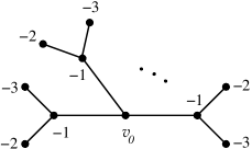
Figure 1. The plumbing diagram of the $n$-fold connected sum of the (right-handed) trefoil knot in $S^{3}$. The valency of the central vertex $v_{0}$ is assumed to be $n\in{\mathbb{N}}$, and each edge emanating from $v_{0}$ connects it to a vertex with framing $(-1)$. Furthermore these $(-1)$-vertices are connected to a $(-2)$- and a $(-3)$-framed leaf of the graph. Regarding $v_{0}$ as a circle in the plumbed 3-manifold defined by the rest of the graph, it can be identified with the $n$-fold connected sum of the trefoil knot in $S^{3}$.

As an application of the connected sum formula, in an Appendix we give an alternative proof of the following result of Némethi.

Theorem 1.4.

[10, Proposition 3.4.2] Suppose that the two negative definite plumbing trees (or forests) $G_{1}$ and $G_{2}$ define diffeomorphic 3-manifolds $Y_{G_{1}}$ and $Y_{G_{2}}$. Then the lattice homology ${\mathbb{HF}}^{-}(G_{1})$ of $G_{1}$ is isomorphic to the lattice homology ${\mathbb{HF}}^{-}(G_{2})$ of $G_{2}$. In other words, the lattice homology is an invariant of the 3-manifold defined by the plumbing graph.

The paper is organized as follows. In Section 2 we review the basics of lattice homology for negative definte graphs. In Sections 3 and 4 we introduce the knot filtration on the lattice chain complex of the background graph, describe the master complex and verify the connected sum formula. In Section 5 we show how to apply this information to determine the lattice homology of graphs we get by attaching various framings to the distinguished point $v_{0}$. In Section 6 we determine the knot filtration in one specific example, and verify Theorem 1.2. Finally in Section 7 we give a proof of Theorem 1.4 (another proof appeared in [12]), and in Section 8 we reprove a further result of Némethi [10] stating that lattice homology is finitely generated as an $\mathbb{F}[U]$-module.

Notation

Suppose that $\Gamma$ is a tree (or forest), and $G$ is the same graph equipped with framings, i.e. we attach integers to the vertices of $\Gamma$. The plumbing of disk bundles over spheres defined by $G$ will be denoted by $X_{G}$, and its boundary 3-manifold is $Y_{G}$. Let $M_{G}$ denote the incidence matrix associated to $G$ (with framings in the diagonal). This matrix presents the intersection form of $X_{G}$ in the basis provided by the vertices of the plumbing graph.

Suppose that $\Gamma_{v_{0}}$ is a plumbing tree (or forest) with a distinguished vertex $v_{0}$ which is left unframed (but all other vertices of $\Gamma_{v_{0}}$ are framed). Let $G$ denote the plumbing graph we get by deleting the vertex $v_{0}$ (and all the edges adjacent to it). We will always assume that the plumbing trees/forests we work with are negative definite.

Remark 1.5.

We can regard the unknot defined by $v_{0}$ in the plumbing picture as a (not necessarily trivial) knot in the plumbed 3-manifold $Y_{G}$.

Recall that for a negative definite tree (or forest) $G$ on the vertex set $\mathrm{Vert}(G)$ the vertex $v\in\mathrm{Vert}(G)$ is a bad vertex if $m_{v}+d_{v}>0$, where $m_{v}$ denotes the framing attached to $v$ while $d_{v}$ is the valency or degree of $v$ (the number of edges emanating from $v$). A vertex is good if it is not bad, that is, $m_{v}+d_{v}\leq 0$.

Acknowledgements: PSO was supported by NSF grant number DMS-0804121. AS was supported by OTKA NK81203, by the ERC Grant LDTBud, by Lendület program and by the Institute for Advanced Study. ZSz was supported by NSF grants DMS-0603940, DMS-0704053 and DMS-1006006.

2. Review of lattice homology

Lattice homology has been introduced by Némethi in [10] (cf. also [11, 12, 13]). In this section we review the basic notions and concepts of this theory. Our main purpose is to set up notations which will be used in the rest of the paper.

Following [10], for a given negative definite plumbing tree $G$ we define a $\mathbb{Z}$-graded combinatorial chain complex $({\mathbb{CF}}^{\infty}(G),\partial)$ (and then a subcomplex $({\mathbb{CF}}^{-}(G),\partial)$ of it), which is a module over the ring of Laurent polynomials $\mathbb{F}[U^{-1},U]$ (and over the polynomial ring $\mathbb{F}[U]$, respectively), where we assume for simplicity that $\mathbb{F}={\mathbb{Z}}/{2}{\mathbb{Z}}$.

Define $Char(G)$ as the set of characteristic cohomology elements of $H^{2}(X_{G};\mathbb{Z})$, that is,

$$Char(G)=\{K\colon H_{2}(X_{G};\mathbb{Z})\to\mathbb{Z}\mid K(x)\equiv x\cdot x\pmod{2}\}.$$

The lattice chain complex ${\mathbb{CF}}^{\infty}(G)$ is freely generated over $\mathbb{F}[U^{-1},U]$ by the product $\mathrm{Char}(G)\times{\mathbb{P}}(\mathrm{Vert}(G))$, that is, by elements $[K,E]$ where $K\in\mathrm{Char}(G)\subset H^{2}(X_{G};\mathbb{Z})$ and $E\subset\mathrm{Vert}(G)$. We introduce a $\mathbb{Z}$-grading on this complex, called the $\delta$-grading, which is defined on the generator $[K,E]$ as the number of elements in $E$. To define the boundary map of the chain complex, we proceed as follows. Given a subset $I\subset E$, we define the $G$-weight $f([K,I])$ as the quantity

(2.1) $$2f([K,I])=\left(\sum_{v\in I}K(v)\right)+\left(\sum_{v\in I}v\right)\cdot\left(\sum_{v\in I}v\right).$$

Remark 2.1.

Using the fact that $G$ is negative definite, the integer $f([K,I])$ can be easily shown to be equal to

$$\frac{1}{8}\left((K+\sum_{v\in I}2v^{*})^{2}-K^{2}\right),$$

where $v^{*}\in H^{2}(X_{G},Y_{G};\mathbb{Z})$ denotes the Poincaré dual of the class $v\in H_{2}(X_{G};\mathbb{Z})$ corresponding to the vertex $v\in\mathrm{Vert}(G)$. This form of $f(K,I)$ immediately implies, for example, the following useful identity: if $I\subset E$ then

(2.2) $$f([K,I])-f([-K-\sum_{u\in E}2u^{*},E-I])=f([K,E]).$$

We define the minimal $G$-weight $g([K,E])$ of $[K,E]$ by the formula

$$g([K,E])=\min\{f([K,I])\mid{I\subset E}\}.$$

The quantities $A_{v}([K,E])$ and $B_{v}([K,E])$ are defined as follows:

$$A_{v}([K,E])=g([K,E-v]) B_{v}([K,E])=\min\{f([K,I])\mid{v\in I\subset E}\}.$$ and

A simple argument shows that

(2.3) $$B_{v}([K,E])=\left(\frac{K(v)+v^{2}}{2}\right)+g([K+2v^{*},E-v]).$$

It follows trivially from the definition that

$$\min\{A_{v}([K,E]),B_{v}([K,E])\}=g([K,E]).$$

Now we define the boundary map $\partial\colon{\mathbb{CF}}^{\infty}(G)\to{\mathbb{CF}}^{\infty}(G)$ by the formula:

$${\partial[K,E]}=\sum_{v\in E}U^{a_{v}[K,E]}\otimes[K,E-v]+\sum_{v\in E}U^{b_{v}[K,E]}\otimes[K+2v^{*},E-v],$$

where

$$a_{v}[K,E]=A_{v}([K,E])-g([K,E]) b_{v}[K,E]=B_{v}([K,E])-g([K,E]).$$ and

(Extend this map $U$-equivariantly to the terms $U^{j}\otimes[K,E]$ and then linearly to ${\mathbb{CF}}^{\infty}(G)$.) Notice that $a_{v}[K,E],b_{v}[K,E]$ are both nonnegative integers and $\min\{a_{v}[K,E],b_{v}[K,E]\}=0$ follows directly form the definitions. It is obvious that the boundary map decreases the $\delta$-grading by one. Furthermore, it is a simple exercise to show that

Lemma 2.2.

The map $\partial$ is a boundary map, that is, $\partial^{2}=0$.

Proof.

The proof boils down to matching the exponents of the $U$-factors in front of various terms in $\partial^{2}[K,E]$ for a given generator $[K,E]$. This idea leads us to four equations to check. One of them, for example, relates the two $U$-powers in front of the two appearances $[K,E-v_{1}-v_{2}]$ in $\partial^{2}[K,E]$. We claim that

(2.4) $$a_{v_{1}}[K,E]+a_{v_{2}}[K,E-v_{1}]=a_{v_{2}}[K,E]+a_{v_{1}}[K,E-v_{2}]$$

holds, therefore (over $\mathbb{F}$) the two terms cancel each other. Writing out the definitions of the terms in (2.4) we get

$$g([K,E-v_{1}])-g([K,E])+g([K,E-v_{1}-v_{2}])-g([K,E-v_{1}])=$$

$$=g([K,E-v_{2}])-g([K,E])+g([K,E-v_{1}-v_{2}])-g([K,E-v_{2}]),$$

which trivially holds. The remaing three cases to check are:

(2.5) $$a_{v_{1}}[K,E]+b_{v_{2}}[K,E-v_{1}]=b_{v_{2}}[K,E]+a_{v_{1}}[K+2v_{2}^{*},E-v_{2}],$$

$$b_{v_{1}}[K,E]+a_{v_{2}}[K+2v_{1}^{*},E-v_{1}]=a_{v_{2}}[K,E]+b_{v_{1}}[K,E-v_{2}],$$

and finally

$$b_{v_{1}}[K,E]+b_{v_{2}}[K+2v_{1}^{*},E-v_{1}]=b_{v_{2}}[K,E]+b_{v_{1}}[K+2v_{2}^{*},E-v_{2}].$$

Using the definition of $B_{v}$ given in (2.3), the equations reduce to similar equalities as in the first case. ∎

Remark 2.3.

In [10] the theory is set up over $\mathbb{Z}$; for simplicity in the present paper we use the coefficients from the field $\mathbb{F}=\mathbb{Z}/2\mathbb{Z}$ of two elements.

2.1. Connected sums

Suppose that the plumbing forest $G$ is the union of $G_{1}$ and $G_{2}$, with no edges connecting any vertex of $G_{1}$ to any vertex of $G_{2}$. (In other words, $G_{1}$ and $G_{2}$ are both unions of components of $G$.) It is a simple topological fact that in this case $Y_{G}$ decomposes as the connected sum of the two 3-manifolds $Y_{G_{1}}$ and $Y_{G_{2}}$. Correspondingly, the $\mathbb{F}[U^{-1},U]$-module ${\mathbb{CF}}^{\infty}(G)$ decomposes as the tensor product

(2.6) $${\mathbb{CF}}^{\infty}(G)\cong{\mathbb{CF}}^{\infty}(G_{1})\otimes_{\mathbb{F}[U^{-1},U]}{\mathbb{CF}}^{\infty}(G_{2}),$$

and the definition of the boundary map $\partial$ shows that this decomposition holds on the chain complex level as well.

2.2. Spin^c structures and the $J$-map

Define an equivalence relation for the generators of the chain complex ${\mathbb{CF}}^{\infty}(G)$ as follows: we say that $[K,E]$ and $[K^{\prime},E^{\prime}]$ are equivalent if $K-K^{\prime}\in 2H^{2}(X_{G},Y_{G};\mathbb{Z})$. Obviously, the boundary map respects this equivalence relation, hence the chain complex splits according to this relation.

It is easy to see that (since $X_{G}$ is simply connected) a characteristic cohomology class $K\in H^{2}(X_{G};\mathbb{Z})$ uniquely determines a spin^c structure on $X_{G}$. By restricting this structure to the boundary 3-manifold $Y_{G}$ we conclude that $K$ naturally induces a spin^c structure $\mathbf{s}_{K}$ on $Y_{G}$. Two classes $K,K^{\prime}$ induce the same spin^c structure on $Y_{G}$ if and only if they are equivalent in the above sense (that is, $K-K^{\prime}\in 2H^{2}(X_{G},Y_{G};\mathbb{Z})$). Therefore the splitting of the chain complex ${\mathbb{CF}}^{\infty}(G)$ described above is parametrized by the spin^c structures of $Y_{G}$:

$${\mathbb{CF}}^{\infty}(G)=\sum_{\mathbf{s}\in Spin^{c}(Y_{G})}{\mathbb{CF}}^{\infty}(G,\mathbf{s}),$$

where ${\mathbb{CF}}^{\infty}(G,\mathbf{s})$ is spanned by those pairs $[K,E]$ for which $\mathbf{s}_{K}=\mathbf{s}$.

Consider the map

$$J[K,E]=[-K-\sum_{v\in E}2v^{*},E]$$

and extend it $U$-equivariantly (and linearly) to ${\mathbb{CF}}^{\infty}(G)$. Obviously $J$ provides an involution on ${\mathbb{CF}}^{\infty}(G)$, and a simple calculation shows the following:

Lemma 2.4.

The $J$-map is a chain map, that is, $J\circ\partial=\partial\circ J$.

Proof.

The two compositions can be easily determined as

$$(J\circ\partial)[K,E]=\sum_{v\in E}\left(U^{a_{v}[K,E]}\otimes[-K-\sum_{u\in E-v}2u^{*},E-v]\right)+$$

$$\sum_{v\in E}\left(U^{b_{v}[K,E]}\otimes[-K-\sum_{u\in E}2u^{*},E-v]\right)$$

and

$$(\partial\circ J)[K,E]=\sum_{v\in E}\left(U^{a_{v}[-K-\sum_{u\in E}2u^{*},E]}\otimes[-K-\sum_{u\in E}2u^{*},E-v]\right)+$$

$$+\sum_{v\in E}\left(U^{b_{v}[-K-\sum_{u\in E}2u^{*},E]}\otimes[-K-\sum_{u\in E-v}2u^{*},E-v]\right).$$

The fact that $J$ is a chain map, then follows from the two identities

(2.7) $$a_{v}[K,E]=b_{v}[-K-\sum_{u\in E}2u^{*},E]\qquad{\mbox{and}}\qquad a_{v}[-K-\sum_{u\in E}2u^{*},E]=b_{v}[K,E].$$

In turn, these identities easily follow from the identity of  (2.2), concluding the proof of the lemma. ∎

The $J$-map obviously respects the splitting of ${\mathbb{CF}}^{\infty}(G)$ according to spin^c structures. In fact, the spin^c structures represented by $K$ and $-K$ are ’conjugate’ to each other as spin^c structures on $Y_{G}$ (cf. [19]), inducing the spin^c structures $\mathbf{s},{\overline{\mathbf{s}}}\in$Spin${}^{c}(Y_{G})$, respectively. The $J$-map therefore is just the manifestation of the conjugation involution of spin^c structures on the chain complex level. Indeed, $J$ provides an isomorphism between the two subcomplexes ${\mathbb{CF}}^{\infty}(G,\mathbf{s})$ and ${\mathbb{CF}}^{\infty}(G,{\overline{\mathbf{s}}})$.

2.3. Gradings

The lattice chain complex ${\mathbb{CF}}^{\infty}(G)$ admits a Maslov grading: for a generator $[K,E]$ and $j\in{\mathbb{Z}}$ define ${\rm{gr}}(U^{j}\otimes[K,E])$ by the formula:

$${\rm{gr}}(U^{j}\otimes[K,E])=-2j+2g([K,E])+|E|+\frac{1}{4}(K^{2}+|\mathrm{Vert}(G)|).$$

Recall that $K^{2}$ is defined as the square of $nK$ divided by $n^{2}$, where $nK\in H^{2}(X_{G},Y_{G};\mathbb{Z})$, hence it admits a cup square. (Here we use the fact that $G$ is negative definite, hence $\det M_{G}\neq 0$, so the restriction of any cohomology class from $X_{G}$ to its boundary $Y_{G}$ is torsion.) We expect ${\rm{gr}}(U^{j}\otimes[K,E])$ to be a rational number rather than an integer.

Lemma 2.5.

The boundary map decreases the Maslov grading by one.

Proof.

We proceed separately for the two types of components of the boundary map. After obvious simplifications we get that

$${\rm{gr}}(U^{j}\otimes[K,E])-{\rm{gr}}(U^{j}\cdot U^{a_{v}[K,e]}\otimes[K,E-v])=$$

$$2g([K,E])+|E|+2a_{v}[K,E]-2g([K,E-v])-|E-v|,$$

which, according to the definition of $a_{v}[K,E]$, is equal to 1. Similarly,

$${\rm{gr}}(U^{j}\otimes[K,E])-{\rm{gr}}(U^{j}\cdot U^{b_{v}[K,e]}\otimes[K+2v^{*},E-v])=1$$

follows from the same simplifications and Equation (2.3). ∎

It is not hard to see that the $J$-map preserves the Maslov grading. Indeed,

$${\rm{gr}}([K,E])-{\rm{gr}}(J[K,E])={\rm{gr}}([K,E])-{\rm{gr}}([-K-\sum_{v\in E}2v^{*},E])=$$

$$=2g([K,E])-2g([-K-\sum_{v\in E}2v^{*},E])+\frac{1}{4}(K^{2}-(-K-\sum_{v\in E}2v^{*})^{2}).$$

Using the idenity of (2.2) and the alternative definition of $f(K,E)$, it follows that the above difference is equal to zero.

Recall that the cardinality $|E|$ for a generator $[K,E]$ of ${\mathbb{CF}}^{-}(G)$ gives the $\delta$-grading, which decomposes each ${\mathbb{CF}}^{-}(G,\mathbf{s})$ as

$${\mathbb{CF}}^{-}(G,\mathbf{s})=\oplus_{k=0}^{n}{\mathbb{CF}}^{-}_{k}(G,\mathbf{s}),$$

where $n=|\mathrm{Vert}(G)|$. It is easy to see that the differential $\partial$ decreases $\delta$-grading by one.

2.4. Definition of the lattice homology

We define the lattice homology groups as follows. Consider $({{{\mathbb{CF}}^{\infty}}}(G),\partial)$, and let $({{{\mathbb{CF}}^{-}}}(G),\partial)$ denote the subcomplex generated by those generators $U^{j}\otimes[K,E]$ for which $j\geq 0$ (and equipped with the differential restricted to the subspace). Setting $U=0$ in this subcomplex we get the complex $({{\widehat{\mathbb{CF}}}}(G),{\widehat{\partial}})$. Obviously all these chain complexes split according to spin^c structures and admit a Maslov grading, $\delta$-grading and a $J$-map.

Definition 2.6.

Let us define the lattice homology ${\mathbb{HF}}^{\infty}(G)$ as the homology of the chain complex $({{{\mathbb{CF}}^{\infty}}}(G),\partial)$. The homology of the subcomplex ${{{\mathbb{CF}}^{-}}}(G)$ (with the boundary map $\partial$ restricted to it) will be denoted by ${\mathbb{HF}}^{-}(G)$, while the homology of $({{\widehat{\mathbb{CF}}}}(G),{\widehat{\partial}})$ is $\widehat{\mathbb{HF}}(G)$.

Since the chain complex ${\mathbb{CF}}^{-}(G)$ (and similarly, ${\mathbb{CF}}^{\infty}(G)$ and $\widehat{\mathbb{CF}}(G)$) splits according to spin^c structures, so does the homology, giving the decomposition

$${\mathbb{HF}}^{-}(G)=\oplus_{\mathbf{s}\in{\rm{Spin}}^{c}(Y_{G})}{\mathbb{HF}}^{-}(G,\mathbf{s}).$$

The $\delta$-grading then decomposes ${\mathbb{HF}}^{-}(G,\mathbf{s})$ further as

$${\mathbb{HF}}^{-}(G,\mathbf{s})=\oplus_{k=0}^{n}{\mathbb{HF}}^{-}_{k}(G,\mathbf{s}),$$

where $n=|\mathrm{Vert}(G)|$. The Maslov grading provides an additional ${\mathbb{Q}}$-grading on ${\mathbb{HF}}^{-}(G,\mathbf{s})$, but we reserve the subscript ${\mathbb{HF}}^{-}_{k}(G,\mathbf{s})$ for the $\delta$-grading.

Remark 2.7.

The embedding $i\colon{\mathbb{CF}}^{-}(G)\to{\mathbb{CF}}^{\infty}(G)$ can be used to define a quotient complex ${\mathbb{CF}}^{+}(G)$ (with the differential inherited from this construction) which fits into the short exact sequence

$$0\to{\mathbb{CF}}^{-}(G)\to{\mathbb{CF}}^{\infty}(G)\to{\mathbb{CF}}^{+}(G)\to 0.$$

The homology of this quotient complex will be denoted by ${\mathbb{HF}}^{+}(G)$. The same splittings as before (according to spin^c structures, the $\delta$-grading and Maslov grading) apply to this theory is well. The short exact sequence above then induces a long exact sequence on the various homologies.

In a similar manner, ${\mathbb{CF}}^{-}(G)$ and $\widehat{\mathbb{CF}}(G)$ can be also connected by a short exact sequence:

$$0\to{\mathbb{CF}}^{-}(G)\stackrel{{\scriptstyle U}}{{\to}}{\mathbb{CF}}^{-}(G)\to\widehat{\mathbb{CF}}(G)\to 0,$$

where the first map is multiplication by $U$. This short exact sequence then induces a long exact sequence on homologies connecting ${\mathbb{HF}}^{-}(G)$ and $\widehat{\mathbb{HF}}(G)$:

$$\ldots\to{\mathbb{HF}}^{-}_{q}(G)\stackrel{{\scriptstyle U}}{{\to}}{\mathbb{HF}}^{-}_{q}(G)\to\widehat{\mathbb{HF}}_{q}(G)\to{\mathbb{HF}}^{-}_{q-1}\to\ldots$$

2.5. The structure of ${\mathbb{HF}}^{-}(G)$

The homology group ${\mathbb{HF}}^{-}(G)$ is obviously an $\mathbb{F}[U]$-module. In the next result we describe an algebraic property these particular modules satisfy.

Theorem 2.8.

(Némethi, [10]) Suppose that $G$ is a negative definite plumbing tree and $\mathbf{s}$ is a spin^c structure on $Y_{G}$. Then the homology ${\mathbb{HF}}^{-}(G,\mathbf{s})$ is a finitely generated $\mathbb{F}[U]$-module of the form

$${\mathbb{HF}}^{-}(G,\mathbf{s})=\mathbb{F}[U]\oplus\bigoplus_{i}A_{i},$$

where the modules $A_{i}$ are cyclic modules of the form $\mathbb{F}[U]/(U^{n})$. Furthermore the $\mathbb{F}[U]$-factor is in ${\mathbb{HF}}^{-}_{0}(G,\mathbf{s})$.

The proof of the fact that ${\mathbb{HF}}^{-}(G,\mathbf{s})$ is finitely generated (as an $\mathbb{F}[U]$-module) is deferred until Section 8. Here we show how the previous discussion and this finite generation implies the rest of the structure theorem.

Since any finitely generated $\mathbb{F}[U]$-module is the direct sum of cyclic $\mathbb{F}[U]$-modules, in verifying Theorem 2.8 we need to show that

• the $U$-torsion parts of ${\mathbb{HF}}^{-}(G,\mathbf{s})$ are all of the form $\mathbb{F}[U]/(U^{n})$ and

• there is a single non-torsion module $\mathbb{F}[U]$ in ${\mathbb{HF}}^{-}(G,\mathbf{s})$, and it lives in $\delta$-degree 0.

The first claim follows easily from the existence of a Maslov grading and the fact that multiplication by $U$ drops this grading by $-2$: these facts imply that the ideal $I$ in $A_{i}=\mathbb{F}[U]/I$ should be generated by a homogeneous polynomial, implying that $I=(U^{n})$ for some $n$.

For the second claim we define a further chain complex $(\overline{\mathbb{CF}}(G),{\overline{\partial}})$ associated to $G$ by setting $U=1$ in the chain complex ${{{\mathbb{CF}}^{-}}}(G)$ (or in ${\mathbb{CF}}^{\infty}(G,\mathbf{s})$). Then $\overline{\mathbb{CF}}(G)$ is generated by the pairs $[K,E]\in\mathrm{Char}(G)\times{\mathbb{P}}(\mathrm{Vert}(G))$ over $\mathbb{F}$ (just like $\widehat{\mathbb{CF}}(G)$ is), but the boundary map ${\overline{\partial}}$ is radically different from ${\widehat{\partial}}$. While in ${\widehat{\partial}}$ we allow nontrivial boundary if and only if $a_{v}$ (or $b_{v}$) is equal to 0, in ${\overline{\partial}}$ the information captured by $a_{v}$ and $b_{v}$ is completely lost. Therefore it is not surprising that

Lemma 2.9.

For a fixed spin^c structure $\mathbf{s}$ the homology $\overline{\mathbb{HF}}(G,\mathbf{s})$ of $\overline{\mathbb{CF}}(G,\mathbf{s})$ is isomorphic to $\mathbb{F}$, and $\overline{\mathbb{HF}}(G,\mathbf{s})=\overline{\mathbb{HF}}_{0}(G,\mathbf{s})$.

Proof.

By considering the set of pairs $[K,E]$ with spin^c structure $\mathbf{s}_{K}=\mathbf{s}$, the corresponding hypercubes

$$\{K+\sum_{v_{i}\in E}2t_{i}v_{i}^{*}|t_{i}\in[0,1]\}$$

(when viewed $H^{*}(X_{G};\mathbb{Z})$ as subset of $H^{*}(X_{G};\mathbb{R})\cong\mathbb{R}^{n}$) provide a $CW$-decomposition of ${\mathbb{R}}^{n}$. It follows from the definition that $H_{*}(\overline{\mathbb{CF}}(G,\mathbf{s}),{\overline{\partial}})$ simply computes the $CW$-homology of ${\mathbb{R}}^{n}$, which is equal (with $\mathbb{F}$-coefficients) to $\mathbb{F}$ in degree 0. (Despite its simplicity, the $U=1$ theory turns out to be useful in particular explicit computations.) ∎

Proof of Theorem 2.8, assuming the finiteness claim.

Suppose that ${\mathbb{HF}}^{-}(G,\mathbf{s})$ is a finitely generated $\mathbb{F}[U]$-module. We will appeal to the Universal Coefficient Theorem: notice that $\mathbb{F}$ is an $\mathbb{F}[U]$-module by defining the action of the polynomial $p(U)=\sum p_{i}U^{i}$ as multiplication by $\sum p_{i}$. Then

$$0\to{\mathbb{HF}}^{-}_{q}(G,\mathbf{s})\otimes_{\mathbb{F}[U]}\mathbb{F}\to\overline{\mathbb{HF}}_{q}(G,\mathbf{s})\to Tor({\mathbb{HF}}^{-}_{q-1}(G,\mathbf{s}),\mathbb{F})\to 0$$

proves the claim by the previos computation of $\overline{\mathbb{HF}}(G,\mathbf{s})$ and the facts that $Tor(\mathbb{F}[U],\mathbb{F})=Tor(\mathbb{F}[U]/U^{n},\mathbb{F})=0$ and that $\mathbb{F}[U]/(U^{n})\otimes_{\mathbb{F}[U]}\mathbb{F}=0$, while $\mathbb{F}[U]\otimes_{\mathbb{F}[U]}\mathbb{F}=\mathbb{F}$. ∎

Corollary 2.10.

The $\mathbb{F}[U^{-1},U]$-module ${\mathbb{HF}}^{\infty}(G,\mathbf{s})={\mathbb{HF}}^{\infty}_{0}(G,\mathbf{s})$ is isomorphic to $\mathbb{F}[U^{-1},U]$.

Proof.

By the Universal Coefficient Theorem we get that there is a short exact sequence

$$0\to{\mathbb{HF}}^{-}_{q}(G,\mathbf{s})\otimes_{\mathbb{F}[U]}\mathbb{F}[U^{-1},U]\to{\mathbb{HF}}^{\infty}_{q}(G,\mathbf{s})\to Tor({\mathbb{HF}}^{-}_{q-1}(G,\mathbf{s}),\mathbb{F}[U^{-1},U])\to 0.$$

Since $Tor(\mathbb{F}[U],\mathbb{F}[U^{-1},U])=Tor(\mathbb{F}[U]/(U^{n}),\mathbb{F}[U^{-1},U])=0$ and $(\mathbb{F}[U]/(U^{n}))\otimes_{\mathbb{F}[U]}\mathbb{F}[U^{-1},U]=0$, while $\mathbb{F}[U]\otimes_{\mathbb{F}[U]}\mathbb{F}[U^{-1},U]=\mathbb{F}[U^{-1},U]$, the claim obviously follows. By Lemma 2.9 we get that the (single) $\mathbb{F}[U]$-factor is in ${\mathbb{HF}}^{-}_{0}(G,\mathbf{s})$, we get that ${\mathbb{HF}}^{\infty}(G,\mathbf{s})={\mathbb{HF}}^{\infty}_{0}(G,\mathbf{s})$. ∎

Definition 2.11.

Let ${\mathbb{HF}}^{-}_{red}(G,\mathbf{s})\subseteq{\mathbb{HF}}^{-}(G,\mathbf{s})$ denote the kernel of the map $i_{*}$ induced by the embedding $i\colon{\mathbb{CF}}^{-}(G,\mathbf{s})\to{\mathbb{CF}}^{\infty}(G,\mathbf{s})$. This group is finite dimensional as a vector space over $\mathbb{F}$ and is called the reduced lattice homology of $(G,\mathbf{s})$.

2.6. Examples

We conclude this section by working out a simple example which will be useful in our later discussions.

Example 2.12.

Suppose that the tree $G$ has a single vertex $v$ with framing $-1$. The chain complex ${\mathbb{CF}}^{\infty}(G)$ is generated over $\mathbb{F}[U^{-1},U]$ by the elements

$$\{[2n+1,\{v\}],[2n+1,\emptyset]\mid n\in\mathbb{Z}\},$$

where a characteristic vector on $G$ is denoted by its value $2n+1$ on $v$. The boundary map on $[2n+1,\emptyset]=[2n+1]$ is given by $\partial[2n+1]=0$ and by

$$\partial[2n+1,\{v\}]=\left\{\begin{array}[]{ll}[2n+1]+U^{n}\otimes[2n-1]&{\text{if $n\geq 0$}}\\ U^{-n}\otimes[2n+1]+[2n-1]&{\text{if $n<0$}}.\end{array}\right.$$

These formulae also describe the chain complexes ${\mathbb{CF}}^{-}(G)$ and $\widehat{\mathbb{CF}}(G)$ (generated over $\mathbb{F}[U]$ and over $\mathbb{F}$). Let us consider the map $F$ from ${\mathbb{CF}}^{\infty}(G)$ to the subcomplex $\mathbb{F}[U^{-1},U]\langle[-1]\rangle\subseteq{\mathbb{CF}}^{\infty}(G)$ generated by the element $[-1]$, defined as

$$F([2n+1,E])=\left\{\begin{array}[]{ll}0&{\text{if $E=\{v\}$}}\\ U^{\frac{1}{2}n(n+1)}\otimes[-1]&{\text{if $E=\emptyset$}}\end{array}\right.$$

This map provides a chain homotopy equivalence between ${\mathbb{CF}}^{\infty}(G)$ and $\mathbb{F}[U^{-1},U]$ (the latter equipped with the differential $\partial=0$), as shown by the chain homotopy

$$H([2n+1,E])=\left\{\begin{array}[]{ll}0&{\text{if $E=\{v\}$ or $n=-1$}}\\ \sum_{i=0}^{n}U^{s_{i}}\otimes[2(n-i)+1,v]&{\text{if $E=\emptyset$ and $n\geq 0$}}\\ \sum_{i=0}^{-n-2}U^{r_{i}}\otimes[2(n+i+1)+1,v]&{\text{if $E=\emptyset$ and $n<-1$}}\\ \end{array}\right.$$

where $s_{0}=0$ and $s_{i}=s_{i-1}+b_{v}[2(n-i-1)-1,v]=\frac{1}{2}i(2n+1-i)$, $r_{0}=0$ and $r_{i}=r_{i-1}+a_{v}[2(n+i)+1,v]=-\frac{1}{2}i(2n+1+i)$. In conclusion, the homology ${\mathbb{HF}}^{\infty}(G)$ (and similarly ${\mathbb{HF}}^{-}(G)$ and $\widehat{\mathbb{HF}}(G)$) is generated by the class of $[-1]$ over $\mathbb{F}[U^{-1},U]$ (and over $\mathbb{F}[U]$ and $\mathbb{F}$, respectively). In particular, ${\mathbb{HF}}^{-}_{i}(G)=0$ for $i>0$.

Remark 2.13.

A similar computation shows that the lattice homology ${\mathbb{HF}}^{-}(G_{k})$ of the graph $G_{k}$ we get by considering a linear chain of $k$ vertices of framing $(-2)$ and a final one with framing $(-1)$ (cf. Figure 2) is also isomorphic to $\mathbb{F}[U]$ (and to $\mathbb{F}$ in the $\widehat{\mathbb{CF}}$-theory). The above example discusses the case $k=0$ of this family. We will provide details of the computation for further $k$’s in Section 7.

Figure 2. The plumbing tree $G_{k}$. The graph has $k+1$ vertices, the left-most admitting framing $(-1)$ while all the others have framing $(-2)$. It is easy to see that the corresponding 3-manifold is $S^{3}$.

Recall that for the disjoint union $G=G_{1}\cup G_{2}$ of two trees/forests the chain complex of $G$ (and therefore the lattice homology of $G$) splits as the tensor product of the lattice homologies of $G_{1}$ and $G_{2}$ (over the coefficient ring of the chosen theory). As a quick corollary we get

Corollary 2.14.

Suppose that $G=G_{1}\cup G_{2}$ where $G_{2}$ is the graph encountered in Example 2.12. Then ${\mathbb{HF}}^{-}(G)\cong{\mathbb{HF}}^{-}(G_{1})$. (Similar statements hold for the other versions of the theory.)

Proof.

By the connected sum formula (Equation (2.6)), and by the computation in Example 2.12 we get that

$${\mathbb{HF}}^{-}(G)\cong{\mathbb{HF}}^{-}(G_{1})\otimes_{\mathbb{F}[U]}{\mathbb{HF}}^{-}(G_{2})\cong{\mathbb{HF}}^{-}(G_{1})\otimes_{\mathbb{F}[U]}{\mathbb{F}[U]}\cong{\mathbb{HF}}^{-}(G_{1}).$$

verifying the statement. ∎

3. The knot filtration on lattice homology

Denote the vertices of the tree $\Gamma_{v_{0}}$ by $V=\mathrm{Vert}(\Gamma_{v_{0}})=\{v_{0},v_{1},\ldots,v_{n}\}$. Assume that each $v_{j}$ with $j>0$ is equipped with a framing $m_{j}\in\mathbb{Z}$, but leave the vertex $v_{0}$ unframed. In the following we will assume that $G=\Gamma_{v_{0}}-v_{0}$ is negative definite. The reason for this assumption is that for more general graphs lattice homology provides groups isomorphic to the corresponding Heegaard Floer homology groups only after completion; in particular after allowing infinite sums in the chain complex. For such elements, however, the definition of any filtration requires more care. To avoid these technical difficulties, here we restrict ourselves to the negative definite case.

For a framing $m_{0}\in\mathbb{Z}$ on $v_{0}$ denote the framed graph we get from $\Gamma_{v_{0}}$ by $G_{v_{0}}=G_{m_{0}}(v_{0})$. (We will always assume that $m_{0}$ is chosen in such a way that $G_{m_{0}}(v_{0})$ is also negative definite.) Let $\Sigma\in H_{2}(X_{G_{v_{0}}};{\mathbb{Q}})$ be a homology class satisfying:

(3.1) $$\Sigma=v_{0}+\sum_{j=1}^{n}a_{j}\cdot v_{j}\quad(\text{where~{}}a_{j}\in{\mathbb{Q}}),\quad{\mbox{and}}\quad v_{j}\cdot\Sigma=0\quad(\text{for all~{}}j>0).$$

Notice that since $G=\Gamma_{v_{0}}-v_{0}$ is assumed to be negative definite, the class $\Sigma$ exists and is unique. In the next two section we will follow the convention that characteristic classes on $G$ and subsets of $V-\{v_{0}\}$ will be denoted by $K$ and $E$ respectively, while the characteristic classes on $G_{v_{0}}$ and subsets of $V$ will be denoted by $L$ and $H$, resp.

Lemma 3.1.

Let us fix a generator $[K,E]\in\mathrm{Char}(G)\times{\mathbb{P}}(V-v_{0})$ of the lattice chain complex ${\mathbb{CF}}^{\infty}(G)$ of $G$. There is a unique element $L=L_{[K,E]}\in\mathrm{Char}(G_{v_{0}})$ with the properties that for $H_{E}=E\cup\{v_{0}\}$

• $L|_{G}=K$ and

• $a_{v_{0}}[L,H_{E}]=b_{v_{0}}[L,H_{E}]=0$.

Proof.

The equality $a_{v_{0}}[L,H_{E}]=b_{v_{0}}[L,H_{E}]$ is, by definition, equivalent to $A_{v_{0}}([L,H_{E}])=B_{v_{0}}([L,H_{E}])$. By its definition $A_{v_{0}}([L,H_{E}])=g([K,E])$ is independent of $L(v_{0})$ (and of the framing $m_{0}=v_{0}^{2}$ of $v_{0}$), while since $K(v_{j})=L(v_{j})$ for $j>0$, by Equation 2.3

$$2B_{v_{0}}([L,H_{E}])=L(v_{0})+v_{0}^{2}+2g([K+2v_{0}^{*},E]).$$

The identity $2A_{v_{0}}([L,H_{E}])=2B_{v_{0}}([L,H_{E}])$ then uniquely specifies $L(v_{0})$:

$$L(v_{0}) =-v_{0}^{2}+2g([K,E])-2g([K+2v_{0}^{*},E])$$

$$=-v_{0}^{2}+\min_{I\subset E}\left(\sum_{v\in I}K(v)+(\sum_{v\in I}v)^{2}\right)-\min_{I\subset E}\left(\sum_{v\in I}K(v)+(\sum_{v\in I}v)^{2}+2v_{0}\cdot(\sum_{v\in I}v)\right).$$

Since $K$ is characteristic, both minima are even, and therefore $L(v_{0})\equiv v_{0}^{2}\mod 2$, implying that $L$ is also characteristic. ∎

Definition 3.2.

We define the Alexander grading $A([K,E])$ of a generator $[K,E]$ of ${\mathbb{CF}}^{\infty}(G)$ by the formula

$$A([K,E])=\frac{1}{2}(L(\Sigma)+\Sigma^{2})\in{\mathbb{Q}},$$

where $L=L_{[K,E]}$ is the extension of $K$ found in Lemma 3.1 and $\Sigma$ is the (rational) homology element in $H_{*}(X_{G_{v_{0}}};{\mathbb{Q}})$ associated to $v_{0}$ in Equation (3.1). (In the above formula we regard $L\in H^{2}(X_{G_{v_{0}}};\mathbb{Z})$ as a cohomology class with rational coefficients.) Notice that since $v_{j}\cdot\Sigma=0$ for all $j>0$, the above expression is equal to $\frac{1}{2}(L(\Sigma)+v_{0}\cdot\Sigma)$.

We extend this grading to expressions of the form $U^{j}\otimes[K,E]$ with $j\in\mathbb{Z}$ by

$$A(U^{j}\otimes[K,E])=-j+A([K,E]).$$

In the definition above we fixed a framing $m_{0}$ on $v_{0}$, and it is easy to see that both the values of $L(v_{0})$ and of $\Sigma^{2}=v_{0}\cdot\Sigma$ depend on this choice.

Lemma 3.3.

The value $A([K,E])$ is independent of the choice of the framing $m_{0}=v_{0}^{2}$ of $v_{0}$.

Proof.

By the identities of Lemma 3.1 it is readily visible that $L(v_{0})$ (and hence $L(\Sigma)$) changes by $-1$ if $v_{0}^{2}$ is replaced by $v_{0}^{2}+1$. Since $\Sigma^{2}$ changes exactly as $v_{0}^{2}$ does, the sum $L(v_{0})+\Sigma^{2}$ (and hence $\frac{1}{2}(L(\Sigma)+\Sigma^{2})$) does not depend on the chosen framing $v_{0}^{2}$ on $v_{0}$. ∎

Since $\Sigma$ is not an integral homology class, there is no reason to expect that $A([K,E])$ is an integer in general. On the other hand, it is easy to see that if $K,K^{\prime}$ represent the same spin^c structure then $A([K,E])-A([K^{\prime},E^{\prime}])$ is an integer: if $K^{\prime}=K+2y^{*}$ (with $y\in H_{2}(X_{G};\mathbb{Z})$) then

$$A([K,E])-A([K^{\prime},E^{\prime}])=\frac{1}{2}(L_{[K,E]}-L_{[K^{\prime},E^{\prime}]})(v_{0})\in\mathbb{Z}$$

since $y\cdot\Sigma=0$ and both $L_{[K,E]}$ and $L_{[K^{\prime},E^{\prime}]}$ are characteristic cohomology classes.

Definition 3.4.

For each spin^c structure $\mathbf{s}$ of $G$ there is a rational number $i_{\mathbf{s}}\in[0,1)$ with the property that mod 1 the Alexander grading $A([K,E])$ for a pair $[K,E]$ with $\mathbf{s}_{K}=\mathbf{s}$ is congruent to $i_{\mathbf{s}}$.

Definition 3.5.

The Alexander grading $A$ of generators naturally defines a filtration $\{{\mathcal{F}}_{i}\}$ on the chain complex ${\mathbb{CF}}^{\infty}(G)$ (which we will still denote by $A$ and will call the Alexander filtration) as follows: an element $x\in{\mathbb{CF}}^{\infty}(G)$ is in ${\mathcal{F}}_{i}$ if every component of $x$ (when written in the $\mathbb{F}$-basis $U^{j}\otimes[K,E]$) has Alexander grading at most $i$. Intersecting the above filtration with the subcomplex ${\mathbb{CF}}^{-}(G)$ we get the Alexander filtration $A$ on ${\mathbb{CF}}^{-}(G)$. Similarly, the definition provides Alexander filtrations on the chain complexes $\widehat{\mathbb{CF}}(G)$ and ${\mathbb{CF}}^{+}(G)$.

Equipped with the Alexander filtration, now $({\mathbb{CF}}^{\infty}(G),\partial)$ is a filtered chain complex, as the next lemma shows.

Lemma 3.6.

The chain complex ${\mathbb{CF}}^{\infty}(G)$ (and similarly, ${\mathbb{CF}}^{-}(G)$ and $\widehat{\mathbb{CF}}(G)$) equipped with the Alexander filtration $A$ is a filtered chain complex, that is, if $x\in{\mathcal{F}}_{i}$ then $\partial x\in{\mathcal{F}}_{i}$.

Proof.

We need to show that for a generator $[K,E]$ the inequality $A(\partial[K,E])\leq A([K,E])$ holds. Recall that $\partial[K,E]$ is the sum of two types of elements. In the following we will deal with these two types separately, and verify a slightly stronger statement for these components.

Let us first consider the component of the boundary of the shape of $U^{a_{v}[K,E]}\otimes[K,E-v]$ for some $v\in E$. We claim that in this case

(3.2) $$A([K,E])-A(U^{a_{v}[K,E]}\otimes[K,E-v])=a_{v}[K+2v_{0}^{*},E]$$

holds, obviously implying that the Alexander grading of this boundary component is not greater than that of $[K,E]$. To verify the identity of (3.2), write $\Sigma$ as $v_{0}+\sum_{j=1}^{n}a_{j}\cdot v_{j}$, and note that twice the left-hand-side of Equation (3.2) is equal to

$$K(\sum_{j=1}^{n}a_{j}\cdot v_{j})+L_{[K,E]}(v_{0})+\Sigma^{2}+2g([K,E-v])-2g([K,E])-K(\sum_{j=1}^{n}a_{j}\cdot v_{j})-L_{[K,E-v]}(v_{0})-\Sigma^{2},$$

which, after the simple cancellations and the extensions found in Lemma 3.1 is equal to

$$2g([K,E])-2g([K+2v_{0}^{*},E])+2g([K,E-v])-2g([K,E])-2g([K,E-v])+2g([K+2v_{0}^{*},E-v].$$

After further cancellations, this expression gives $2a_{v}[K+2v_{0}^{*},E]$, verifying Equation (3.2). Since $a_{v}\geq 0$, Equation (3.2) concludes the argument in this case.

Next we compare the Alexander grading of the term $U^{b_{v}[K,E]}\otimes[K+2v^{*},E-v]$ to $A([K,E])$. Now we claim that

(3.3) $$A([K,E])-A(U^{b_{v}[K,E]}\otimes[K+2v^{*},E-v])=b_{v}[K+2v_{0}^{*},E].$$

As before, after substituting the defining formulae into the terms of twice the left-hand-side of (3.3) we get

$$K(\sum_{j=1}^{n}a_{j}\cdot v_{j})+L_{[K,E]}(v_{0})+\Sigma^{2}+2B_{v}[K,E]-2g([K,E])-$$

$$-(K+2v^{*})(\sum_{j=1}^{n}a_{j}\cdot v_{j})-L_{[K+2v^{*},E-v]}(v_{0})-\Sigma^{2}.$$

From the fact that $v^{*}(\Sigma)=0$ we get that $2v^{*}(\sum_{j=1}^{n}a_{j}\cdot v_{j})=-2v\cdot v_{0}$, hence by considering the form of $B_{v}$ given in (2.3) we get that this term is equal to

$$2g([K,E])-2g([K+2v_{0}^{*},E])+2g([K+2v^{*},E-v])+K(v)+v^{2}+2v\cdot v_{0}-2g([K,E])-$$

$$-2g([K+2v^{*},E-v])+2g([K+2v^{*}+2v_{0}^{*},E-v]),$$

and this expression is obviously equal to $2b_{v}[K+2v_{0}^{*},E]$. Once again, since $b_{v}\geq 0$, the statement of the lemma follows. ∎

Definition 3.7.

We define the filtered chain complex $({\mathbb{CF}}^{\infty}(G),\partial,A)$ (and similarly $({\mathbb{CF}}^{-}(G),\partial,A)$ and $(\widehat{\mathbb{CF}}(G),\partial,A)$) the filtered lattice chain complex of the vertex $v_{0}$ in the graph $\Gamma_{v_{0}}$.

Remark 3.8.

Recall that the chain complex ${\mathbb{CF}}^{-}(G)$ splits according to the spin^c structures of the 3-manifold $Y_{G}$. By intersecting the Alexander filtration with the subcomplexes ${\mathbb{CF}}^{-}(G,\mathbf{s})$ for every spin^c structure $\mathbf{s}$, we get a splitting of the filtered chain complex according to spin^c structures as well. The same remark applies to the ${\mathbb{CF}}^{\infty}$ and $\widehat{\mathbb{CF}}$ theories.

Definition 3.9.

The knot lattice homology ${\mathbb{HFK}}^{-}(\Gamma_{v_{0}})$ (and ${\mathbb{HFK}}^{\infty}(\Gamma_{v_{0}}),\widehat{\mathbb{HFK}}(\Gamma_{v_{0}})$) of $v_{0}$ in the graph $\Gamma_{v_{0}}$ is defined as the homology of the graded object associated to the filtered chain complex $({\mathbb{CF}}^{-}(G),\partial,A)$ (and of $({\mathbb{CF}}^{\infty}(G),\partial,A)$, $(\widehat{\mathbb{CF}}(G),{\widehat{\partial}},A)$ respectively). As before, the groups ${\mathbb{HFK}}^{-}(\Gamma_{v_{0}})$ (and similarly ${\mathbb{HFK}}^{\infty}(\Gamma_{v_{0}})$ and $\widehat{\mathbb{HFK}}(\Gamma_{v_{0}})$) split according to the spin^c structures of $Y_{G}$, giving rise to the groups ${\mathbb{HFK}}^{-}(\Gamma_{v_{0}},\mathbf{s})$ for $\mathbf{s}\in$Spin${}^{c}(Y_{G})$.

Let us fix a spin^c structure $\mathbf{s}$ on $Y_{G}$. The group ${\mathbb{HFK}}^{-}(\Gamma_{v_{0}},\mathbf{s})$ then splits according to the Alexander gradings as

$$\oplus_{a}{\mathbb{HFK}}^{-}(\Gamma_{v_{0}},\mathbf{s},a),$$

and the components ${\mathbb{HFK}}^{-}(\Gamma_{v_{0}},\mathbf{s},a)$ are further graded by the absolute $\delta$-grading (originated from the cardinality of the set $E$ for a generator $[K,E]$) and by the Maslov grading.

The relation between the Alexander filtration and the $J$-map is given by the following formula:

Lemma 3.10.

$A(J[K,E]))=-A([K-2v_{0}^{*},E])$.

Proof.

Recall that $J[K,E]=[-K-\sum_{v\in E}2v^{*},E]$. With the extension $L$ of $-K-\sum_{v\in E}2v^{*}$ given by Lemma 3.1 (with the convention that $v_{0}^{2}=0$) we have that

$$2A(J[K,E])=(-K-\sum_{v\in E}2v^{*})(\Sigma-v_{0})+L(v_{0})+\Sigma^{2}.$$

Since $v^{*}(\Sigma)=0$, by the definition of $L(v_{0})$ and the identity of Remark 2.1 this expression is equal to

$$-K(\Sigma-v_{0})+2v_{0}\cdot(\sum_{v\in E}v)+\Sigma^{2}+2g[K,E]-2f[K,E]-2g[K-2v_{0}^{*},E]+2f[K-2v_{0}^{*},E].$$

With the same argument the identity

$$2A([K-2v_{0}^{*},E])=K(\Sigma-v_{0})-2v_{0}^{*}(\Sigma-v_{0})+L^{\prime}(v_{0})+\Sigma^{2}=$$

$$=K(\Sigma-v_{0})-\Sigma^{2}+2g[K-2v_{0}^{*},E]-2g[K,E]$$

follows (since $v_{0}\cdot\Sigma=\Sigma^{2}$ and $v_{0}^{2}=0$). Now the identity of the lemma follows from the observation that $f[K,E]-f[K-2v_{0}^{*},E]-v_{0}\cdot(\sum_{v\in E}v)=0$. ∎

Define $J_{v_{0}}\colon{\mathbb{CF}}^{\infty}(G)\to{\mathbb{CF}}^{\infty}(G)$ by the formula

$$[K,E]\mapsto[-K-\sum_{u\in E}2u^{*}-2v_{0}^{*},E],$$

on a generator $[K,E]$ and extend $U$-equivariantly and linearly to ${\mathbb{CF}}^{\infty}(G)$. It is easy to see that $J_{v_{0}}^{2}=Id$. The result of the previous lemma can be restated as

$$A(J_{v_{0}}[K,E])=-A[K,E].$$

This map is similar to the $J$-map, but takes the vertex $v_{0}$ into special account. For the next statement recall from Definition 3.4 the quantity $i_{\mathbf{s}}$ associated to a spin^c structure $\mathbf{s}$ on $G$.

Lemma 3.11.

The map sending the generator $[K,E]\in{\mathbb{CF}}^{\infty}(G,\mathbf{s})$ to $U^{i_{\mathbf{s}}-A([K,E])}J_{v_{0}}[K,E]$ is a chain map.

Proof.

We show first that the application of the above map to $U^{a_{v}[K,E]}\otimes[K,E-v]$ for some $v\in E$ is equal to

$$U^{i_{\mathbf{s}}-A([K,E])}\cdot U^{b_{v}[-K-\sum_{u\in E}2u^{*}-2v_{0}^{*},E]}\otimes[-K-\sum_{u\in E}2u^{*}-2v_{0}^{*}+2v^{*},E-v].$$

The identification of $J_{v_{0}}(U^{a_{v}[K,E]}\otimes[K,E])$ with the above term easily follows from the observation that

(3.4) $$a_{v}[K,E]+i_{\mathbf{s}}-A([K,E-v])=i_{\mathbf{s}}-A([K,E])+b_{v}[-K-\sum_{u\in E}2u^{*}-2v_{0}^{*}].$$

Equation (3.4), however, is a direct consequence of the equality $b_{v}[-K-\sum_{u\in E}2u^{*}-2v_{0}^{*}]=a_{v}[K+2v_{0}^{*},E]$ and the definitions of the terms describing the Alexander gradings. A similar computation shows the identity for the other type of boundary components (involving the terms of the shape $U^{b_{v}[K,E]}\otimes[K+2v^{*},E-v]$), concluding the proof. ∎

Examples 3.12.

Two examples of the filtered chain complexes associated to certain graphs can be determined as follows.

• Consider first the graph $\Gamma_{v_{0}}$ with two vertices $\{v_{0},v\}$, connected by a single edge, and with $(-1)$ as the framing of $v$. The chain complex of $G=\Gamma_{v_{0}}-v_{0}$ has been determined in Example 2.12. A straightforward calculation shows that $A([2n+1])=n+1$ and

  $$A([2n+1,\{v\}])=\left\{\begin{array}[]{ll}n+1&{\text{if $n\geq 0$}}\\ n&{\text{if $n<0$}}.\end{array}\right.$$

  This formula then describes the Alexander filtration on ${\mathbb{CF}}^{-}(G)$. (Recall that $A(U^{i}\otimes[K,E])=-j+A([K,E])$.) It is easy to see that the chain homotopy encountered in Example 2.12 respects this Alexander filtation, hence the filtered lattice chain complex $({\mathbb{CF}}^{\infty}(G),A)$ is filtered chain homotopic to $\mathbb{F}[U^{-1},U]$, generated by the element $g$ in filtration level 0. In conclusion, $\widehat{\mathbb{HFK}}(\Gamma_{v_{0}})$ and ${\mathbb{HFK}}^{-}(\Gamma_{v_{0}})$ are both generated by the element $[-1]$ (over $\mathbb{F}$ and $\mathbb{F}[U]$, respectively), and the Alexander and Maslov gradings of the generator are both equal to $0$.

• In the second example consider the graph $\Gamma^{\prime}_{v_{0}}$ on the same two vertices $\{v_{0},v\}$, now with no edges at all. (That is, $\Gamma^{\prime}_{v_{0}}$ is given from $\Gamma_{v_{0}}$ by erasing the single edge of $\Gamma_{v_{0}}$.) The background graph $G$ (and hence the chain complex ${\mathbb{CF}}^{-}(G)$) is obviously the same as in the first example, but the Alexander grading $A^{\prime}$ is much simpler now: $A^{\prime}([2n+1])=A^{\prime}([2n+1,\{v\}])=0$ for all $n\in\mathbb{Z}$. Once again, the chain homotopy of Example 2.12 is a filtered chain homotopy, hence we can apply it to determine the filtered lattice chain complex of $\Gamma_{v_{0}}^{\prime}$, concluding that $({\mathbb{CF}}^{\infty}(G),A^{\prime})$ is filtered chain homotopic to $\mathbb{F}[U^{-1},U]$ with the generator in Alexander grading $0$. Once again ${\mathbb{HFK}}^{-}(\Gamma_{v_{0}}^{\prime})$ is generated by $[-1]$.

In conclusion, the filtered chain complexes of the two examples are filtered chain homotopic to each other.

Remark 3.13.

Let $\Gamma^{k}_{v_{0}}$ be constructed from $G_{k}$ of Remark 2.13 by attaching to it the vertex $v_{0}$ together with the edge connecting $v_{0}$ and the single $(-1)$-framed vertex. Minor modifications of the argument above identifies the filtered lattice chain complex of $\Gamma^{k}_{v_{0}}$ with $\mathbb{F}[U^{-1},U]$ (with the generator having Alexander grading 0). We will return to this example in Section 7.

4. The master complex and the connected sum formula

As we will see in the next section, the filtered chain complexes defined in the previous section (together with certain maps, to be discussed below) contain all the relevant information we need for calculating the lattice homologies of graphs we get by attaching various framings to $v_{0}$. The Alexander filtration $A$ on ${\mathbb{CF}}^{\infty}(G)$ can be enhanced to a double filtration by considering the double grading

(4.1) $$U^{j}\otimes[K,E]\mapsto(-j,A(U^{j}\otimes[K,E])).$$

In fact, this doubly filtered chain complex determines (and is determined by) the filtered chain complex $({\mathbb{CF}}^{-}(G),A)$. Notice that multiplication by $U$ decreases Maslov grading by 2, $-j$ by 1 and Alexander grading by 1.

In describing the further structures we need, it is slightly more convenient to work with ${\mathbb{CF}}^{\infty}(G)$, and therefore we will consider the doubly filtered chain complex above. In the following we will find it convenient to equip ${\mathbb{CF}}^{\infty}(G)$ with the following map.

Definition 4.1.

The map $N\colon{\mathbb{CF}}^{\infty}(G)\to{\mathbb{CF}}^{\infty}(G)$ is defined by the formula

(4.2) $$N(U^{j}\otimes[K,E])=U^{i_{s_{K}}-A[K,E]+j}\otimes[K+2v_{0}^{*},E].$$

Notice that $N$ does not preserve the spin^c structure of a given element. Indeed, if $\mathbf{s}_{v_{0}}$ denotes the spin^c structure we get by twisting $\mathbf{s}$ with $v_{0}^{*}$ (and hence we get $c_{1}(\mathbf{s}_{v_{0}^{*}})=c_{1}(\mathbf{s})+2v_{0}^{*}$) then $N$ maps ${\mathbb{CF}}^{\infty}(G,\mathbf{s})$ to ${\mathbb{CF}}^{\infty}(G,\mathbf{s}_{v_{0}})$. In fact, by choosing another rational number $r$ (with $r\equiv i_{\mathbf{s}_{K}}\mod 1$) instead of $i_{\mathbf{s}_{K}}$ in the above formula, we get only multiples of $N$ (multiplied by appropiate monoms of $U$).

Lemma 4.2.

The map $N$ is a chain map, and provides an isomorphism between the chain complex ${\mathbb{CF}}^{\infty}(G,\mathbf{s})$ and ${\mathbb{CF}}^{\infty}(G,\mathbf{s}_{v_{0}^{*}})$.

Proof.

The fact that $N$ is a chain map follows from the identities

(4.3) $$a_{v}[K,E]-A([K,E-v])=a_{v}[K+2v_{0}^{*},E]-A([K,E])$$

and

(4.4) $$b_{v}[K,E]-A([K+2v^{*},E-v])=b_{v}[K+2v_{0}^{*},E]-A([K,E]).$$

These identities follow easily from the definitions of the terms. To show that $N$ is an isomorphism, let the spin^c structure $\mathbf{s}_{-v_{0}^{*}}$ the denoted by $\mathbf{t}$ and consider the map

$$M(U^{j}\otimes[K,E])=U^{A([K-2v_{0}^{*},E])+j-i_{\mathbf{t}}}\otimes[K-2v_{0}^{*},E].$$

$M$ is also a chain map (as the identities similar to (4.3) and (4.4) show), and $M$ and $N$ are inverse maps. It follows therefore that $N$ is an isomorphism between chain complexes. ∎

Notice that $N$ can be written as the composition of the $J$-map with the map $U^{i_{\mathbf{s}}-A([K,E])}J_{v_{0}}[K,E]$ considered in Lemma 3.11.

Definition 4.3.

Suppose that for $i=1,2$ the triples $(C_{i},A_{i},j_{i})$ are doubly filtered chain complexes and $N_{i}\colon C_{i}\to C_{i}$ are given maps. Then the map $f\colon C_{1}\to C_{2}$ is an equivalence of these structures if $f$ is a (doubly) filtered chain homotopy equivalence commuting with $N_{i}$, that is, $f\circ N_{1}=N_{2}\circ f$.

With this definition at hand, now we can define the master complex of $\Gamma_{v_{0}}$ as follows.

Definition 4.4.

Suppose that $\Gamma_{v_{0}}$ is given. Consider ${\mathbb{CF}}^{\infty}(G)$ with the double filtration $(-j,A)$ as above, together with the map $N$ defined in Definition 4.1. The equivalence class of the resulting structure is the master complex of $\Gamma_{v_{0}}$.

As a simple example, a model for the master complex for each of the two cases in Example 3.12 can be easily determined: regarding the map $U^{j}\otimes[K,E]\mapsto(-j,A(U^{j}\otimes[K,E]))$ as a map into the plane, (a representative of) the master complex will have a ${\mathbb{Z}}_{2}$ term for each coordinate $(i,i)$, and all other terms (and all differentials) are zero. In addition, the map $N$ in this model is equal to the identity. (Note that in this case the background 3-manifold is diffeomorphic to $S^{3}$, hence admits a unique spin^c structure.) In short, the master complex for both cases in Example 3.12 is $\mathbb{F}[U^{-1},U]$, with the Alexander grading of $U^{j}$ being equal to $j$ and with $N=id$.

Obviously, by fixing a spin^c structure $\mathbf{s}\in Spin^{c}(Y_{G})$ we can consider the part ${\mathbb{MCF}}^{\infty}(\Gamma_{v_{0}},\mathbf{s})$ of the master complex generated by those elements $U^{j}\otimes[K,E]$ which satisfy the constraint $\mathbf{s}_{K}=\mathbf{s}$. As we noted earlier, $N$ maps components of the master complex corresponding to various spin^c structures into each other.

4.1. The connected sum formula

Suppose that $\Gamma_{v_{0}}$ and $\Gamma^{\prime}_{w_{0}}$ are two graphs with distinguished vertices $v_{0},w_{0}$. Their connected sum is defined in the following:

Definition 4.5.

Let $\Gamma_{v_{0}}$ and $\Gamma^{\prime}_{w_{0}}$ be two graphs with distinguished vertices $v_{0}$ and $w_{0}$. Their connected sum is the graph obtained by taking the disjoint union of $\Gamma_{v_{0}}$ and $\Gamma^{\prime}_{w_{0}}$, and then identifying the distinguished vertices $v_{0}=w_{0}$. The resulting graph

$$\Delta_{(v_{0}=w_{0})}=\Gamma_{v_{0}}\#_{(v_{0}=w_{0})}\Gamma^{\prime}_{w_{0}}$$

(which will be a tree/forest provided both $\Gamma_{v_{0}}$ and $\Gamma^{\prime}_{w_{0}}$ were trees/forests) has a distinguished vertex $v_{0}=w_{0}$.

Remark 4.6.

Notice that this construction gives the connected sum of the two knots specified by $v_{0}$ and $w_{0}$ in the two 3-manifolds $Y_{G}$ and $Y_{G^{\prime}}$.

Recall that for the disjoint graphs $G=\Gamma_{v_{0}}-v_{0}$ and $G^{\prime}=\Gamma^{\prime}_{w_{0}}-w_{0}$ the chain complex ${\mathbb{CF}}^{\infty}(G\cup G^{\prime})$ of their connected sum is simply the tensor product of ${\mathbb{CF}}^{\infty}(G)$ and ${\mathbb{CF}}^{\infty}(G^{\prime})$ (over $\mathbb{F}[U^{-1},U]$). We will denote the Alexander grading/filtration on ${\mathbb{CF}}^{\infty}(G)$ by $A_{v_{0}}$ and on ${\mathbb{CF}}^{\infty}(G^{\prime})$ by $A_{w_{0}}$.

Theorem 4.7.

For the Alexander grading $A_{\#}$ of the generator $[K_{1},E_{1}]\otimes[K_{2},E_{2}]\in{\mathbb{CF}}^{\infty}(G\cup G^{\prime})$ induced by the distinguished vertex $v_{0}=w_{0}$ in $\Delta_{(v_{0}=w_{0})}$ we have that

$$A_{\#}([K_{1},E_{1}]\otimes[K_{2},E_{2}])=A_{v_{0}}([K_{1},E_{1}])+A_{w_{0}}([K_{2},E_{2}]).$$

Proof.

For simplicity fix $v_{0}^{2}=w_{0}^{2}=0$ and consider $\Sigma_{v_{0}}$ and $\Sigma_{w_{0}}$ on the respective sides of the connected sum. By the calculation from Lemma 3.1 it follows that for the extensions $L_{i}$ of $K_{i}$ over the distinguished points $v_{0},w_{0}$, and extension $L$ over $v_{0}=w_{0}$ we have

$$L_{E_{1}\cup E_{2}}(v_{0}=w_{0})=(L_{1})_{E_{1}}(v_{0})+(L_{2})_{E_{2}}(w_{0}).$$

Since $\Sigma^{2}_{v_{0}=w_{0}}=(\Sigma_{v_{0}}+\Sigma_{w_{0}})^{2}=\Sigma^{2}_{v_{0}}+\Sigma^{2}_{w_{0}}$, the above equality shows that both terms of the defining equation of the Alexander grading are additive, concluding the result. ∎

As a corollary, we can now show that

Theorem 4.8.

The master complexes of $\Gamma_{v_{0}}$ and $\Gamma^{\prime}_{w_{0}}$ determine the master complex of the connected sum $\Delta_{(v_{0}=w_{0})}$.

Proof.

As we saw above, the chain complexes for $\Gamma_{v_{0}}$ and $\Gamma^{\prime}_{w_{0}}$ determine the chain complex of $\Delta_{(v_{0}=w_{0})}$ by taking their tensor product. This identity immediately shows that the $j$-filtration on the result is determined by the $j$-filtrations on the components. The content of Theorem 4.7 is that the Alexander filtration on the connected sum is also determined by the Alexander filtrations of the pieces. Finally, the map $N$ is built from the maps $J$ and $J_{v_{0}}$, which simply add for the connected sum, implying the result. A minor adjustment is needed in the last step: if $i_{\mathbf{s}}$ and $i_{\mathbf{s}^{\prime}}$ are the rational numbers determined by Definition 3.4 for the spin^c structures $\mathbf{s}$ and $\mathbf{s}^{\prime}$, then for $\mathbf{s}\#\mathbf{s}^{\prime}$ we take either their sum (if it is in $[0,1)$) or $i_{\mathbf{s}}+i_{\mathbf{s}^{\prime}}-1$. ∎

As a simple application of this formula, consider a graph $\Gamma_{v_{0}}$ and associate to it two further graphs as follows. Both graphs are obtained by adding a further element $e$ to $\mathrm{Vert}(\Gamma_{v_{0}})$, equipped with the framing $(-1)$. We can proceed in the following two ways:

1. Construct $\Gamma_{v_{0}}^{+}$ by adding an edge connecting $e$ and $v_{0}$ to $\Gamma_{v_{0}}$.

2. Define $\Gamma_{v_{0}}^{d}$ by simply adding $e$ (with the fixed framing $(-1)$) without adding any extra edge.

For a pictorial presentation of the two graphs, see Figure 3. It is easy to see that $\Gamma_{v_{0}}^{+}$ is the connected sum of $\Gamma_{v_{0}}$ and the first example in 3.12, while $\Gamma_{v_{0}}^{d}$ is the connected sum of $\Gamma_{v_{0}}$ and the second example of 3.12. Since the master complexes of the two graphs of Example 3.12 coincide, we conclude that

Corollary 4.9.

The master complexes ${\mathbb{MCF}}^{\infty}(\Gamma^{+}_{v_{0}})$ and ${\mathbb{MCF}}^{\infty}(\Gamma^{d}_{v_{0}})$ are equal. In fact, both master complexes are equal to ${\mathbb{MCF}}^{\infty}(\Gamma_{v_{0}})$.

Proof.

Both master complexes are the tensor product (over $\mathbb{F}[U^{-1},U]$) of the master complex of $\Gamma_{v_{0}}$ and of $\mathbb{F}[U^{-1},U]$, concluding the argument. ∎

Figure 3. The two graphs $\Gamma_{v_{0}}^{+}$ (on the left) and $\Gamma_{v_{0}}^{d}$ (on the right) derived from a given graph $\Gamma_{v_{0}}$. The framing of $e$ is $(-1)$ in both cases, and $v_{0}$ is the distinguished vertex (hence admits no framing and is denoted by a hollow circle) in both graphs.

5. Surgery along knots

A formula for computing the lattice homology for the graph $G_{v_{0}}$ (we get from $\Gamma_{v_{0}}$ by attaching appropriate framing to $v_{0}$) can be derived from the knowledge of the master complex of $\Gamma_{v_{0}}$, according to the following result:

Theorem 5.1.

The master complex ${\mathbb{MCF}}^{\infty}(\Gamma_{v_{0}})$ of $\Gamma_{v_{0}}$ determines the lattice homology of the result of the graph obtained by marking $v_{0}$ with any integer $m_{0}\in\mathbb{Z}$, for which the resulting graph is negative definite.

In order to verify this result, first we describe the chain complex computing lattice homology as a mapping cone of related objects. As before, consider the tree $\Gamma_{v_{0}}$ in which each vertex except $v_{0}$ is equipped with a framing. The plumbing graph $G$ is then given by deleting $v_{0}$ from $\Gamma_{v_{0}}$. Let $G_{v_{0}}=G_{n}(v_{0})$ denote the plumbing graph we get from $\Gamma_{v_{0}}$ by attaching the framing $n\in\mathbb{Z}$ to $v_{0}$. Suppose that for the chosen $n$ the graph $G_{v_{0}}$ is negative definite. Our immediate aim is to present the chain complex ${\mathbb{CF}}^{-}(G_{v_{0}})$ as a mapping cone of related objects. These related objects then will be reinterpreted in terms of the master complex ${\mathbb{MCF}}^{\infty}(\Gamma_{v_{0}})$.

Consider the two-step filtration on ${\mathbb{CF}}^{-}(G_{v_{0}})$ where the filtration level of $U^{j}\otimes[L,H]$ is 1 or 0 according to whether $v_{0}$ is in $H$ or $v_{0}$ is not in $H$. Denoting the elements with filtration at most 0 by ${\mathbb{B}}$, we get a short exact sequence

$$0\longrightarrow{\mathbb{B}}\longrightarrow{\mathbb{CF}}^{-}(G_{v_{0}})\longrightarrow{\mathbb{D}}\longrightarrow 0.$$

Explicitly, ${\mathbb{B}}$ is generated by pairs $[L,H]$ with $v_{0}\not\in H$, while a nontrivial element in ${\mathbb{D}}$ can be represented by (linear combinations of) terms $U^{j}\otimes[L,H]$ where $v_{0}\in H$. Indeed, the quotient complex ${\mathbb{D}}$ can be identified with the complex $({\mathbb{T}},\partial_{\mathbb{T}})$, where ${\mathbb{T}}$ is generated over $\mathbb{F}[U]$ by those elements $[L,H]$ of $\mathrm{Char}(G)\times{\mathbb{P}}(V)$ for which $v_{0}\in H$, and

$${\partial_{\mathbb{T}}[L,H]}=\sum_{v\in H-v_{0}}U^{a_{v}[L,H]}\otimes[L,H-v]+\sum_{v\in H-v_{0}}U^{b_{v}[L,H]}\otimes[L+2v^{*},H-v].$$

Notice that there are two obvious maps $\partial_{1},\partial_{2}\colon{\mathbb{T}}\to{\mathbb{B}}$: For a generator $[L,H]$ of ${\mathbb{T}}$ (with $v_{0}\in H$) consider

(5.1) $$\partial_{1}[L,H]=U^{a_{v_{0}}[L,H]}\otimes[L,H-v_{0}],\qquad\partial_{2}[L,H]=U^{b_{v_{0}}[L,H]}\otimes[L+2v_{0}^{*},H-v_{0}].$$

It follows from $\partial^{2}=0$ that both maps $\partial_{1},\partial_{2}\colon{\mathbb{T}}\to{\mathbb{B}}$ are chain maps. It is easy to see that

Lemma 5.2.

The mapping cone of $({\mathbb{T}},{\mathbb{B}},\partial_{1}+\partial_{2})$, is chain homotopic to the chain complex ${\mathbb{CF}}^{-}(G_{n}(v_{0}))$ computing the lattice homology ${\mathbb{HF}}^{-}(G_{n}(v_{0}))$ of the result of $n$-surgery on $v_{0}$. ∎

Next we identify the above terms using the Alexander filtration on ${\mathbb{CF}}^{\infty}(G)$ induced by $v_{0}$. We will use the class $\Sigma$ characterized in Equation (3.1).

Definition 5.3.

Consider the subcomplex $B_{i}\subset{\mathbb{B}}\subset{\mathbb{CF}}^{-}(G_{v_{0}})$ generated by $[L,H]$ where $\frac{1}{2}(L(\Sigma)+\Sigma^{2})=i\in{\mathbb{Q}}$. (Recall that since $[L,H]$ is in ${\mathbb{B}}$, the set $H$ does not contain $v_{0}$. Also, as before, we regard $L\in H^{2}(X_{G_{v_{0}}};\mathbb{Z})$ as a cohomology class with rational coefficients.) Since $v_{j}^{*}(\Sigma)=v_{j}\cdot\Sigma=0$ for all $j\neq 0$, it follows that $B_{i}$ is, indeed, a subcomplex of ${\mathbb{B}}$ for any rational $i$, and obviously $\oplus_{i\in{\mathbb{Q}}}B_{i}={\mathbb{B}}$.

Proposition 5.4.

There is an isomorphism $\varphi\colon B_{i}\to B_{i+1}$.

Proof.

Define the map $\varphi$ by sending a generator $[L,H]$ of $B_{i}$ to $[L^{\prime},H]$ where

$$L^{\prime}(v_{j})=\left\{\begin{array}[]{ll}L(v_{0})+2&{\text{if $j=0$}}\\ L(v_{j})&{\text{if $j\neq 0$}}.\end{array}\right.$$

Since $v_{0}\not\in H$, it follows that $f([L,H])=f([L^{\prime},H])$ (where $f$ is defined in Equation (2.1)), hence the resulting map is an isomorphism between the chain complexes $B_{i}$ and $B_{i+1}$. ∎

Proposition 5.5.

The sum $B=\bigoplus_{0\leq i<1}B_{i}$ is isomorphic to ${\mathbb{CF}}^{-}(G)$.

Proof.

Consider the map $F^{\prime}\colon B\to{\mathbb{CF}}^{-}(G)$ induced by the forgetful map $F^{\prime}$ defined as $[L,H]\mapsto[L|_{G},H]$. It is easy to see that (since $H$ does not contain $v_{0}$) the map $F^{\prime}$ is a chain map. Indeed, $F^{\prime}$ is an isomorphism: one needs to check only that every element $[L|_{G},H]$ admits a unique lift to $[L,H]\in B_{i}$ with $0\leq i<1$. The condition $\frac{1}{2}(L(\Sigma)+\Sigma^{2})=\frac{1}{2}L(v_{0})+\frac{1}{2}(L|_{G})(\Sigma-v_{0})+\frac{1}{2}\Sigma^{2}\in[0,1)$ uniquely characterizes the value of $\frac{1}{2}L(v_{0})$ by the fact that $L(v_{0})\equiv v_{0}^{2}\mod 2$. ∎

Remark 5.6.

Obviously, the same argument shows that $\bigoplus_{r\leq i<r+1}B_{i}$ is isomorphic to ${\mathbb{CF}}^{-}(G)$.

The above statement admits a spin^c-refined version as follows. Notice first that if we fix a spin^c structure $\mathbf{t}$ on the 3-manifold $Y_{G_{v_{0}}}$ we get after the surgery and also fix $i$, then there is a unique spin^c structure $\mathbf{s}$ on $Y_{G}$ induced by $(\mathbf{t},i)$. Indeed, if the cohomology class $L$ satisfies $\mathbf{s}_{L}=\mathbf{t}$ and $\frac{1}{2}(L(\Sigma)+\Sigma^{2})=i$, and $L^{\prime}$ is another representative of $\mathbf{t}$, then

$$L^{\prime}=L+\sum_{i=0}^{n}2n_{i}v_{i}^{*}.$$

In order for $L^{\prime}$ to be also in $B_{i}$, however, the coefficient $n_{0}$ of $v_{0}^{*}$ in the above sum must be equal to zero, hence $L|_{G}$ and $L^{\prime}|_{G}$ represent the same spin^c structure on $Y_{G}$. We will denote this restriction by $(\mathbf{t},i)|_{G}$. Then the above isomorphism $F^{\prime}$ provides

Lemma 5.7.

Let $B_{i}(\mathbf{t})$ be the subcomplex of $B_{i}$ generated by those pairs for which $L$ represents the spin^c structure $\mathbf{t}$. The map $F^{\prime}$ provides an isomorphism between $B_{i}(\mathbf{t})$ and ${\mathbb{CF}}^{-}(G,(\mathbf{t},i)|_{G})$.

Proof.

By the above discussion it is clear that $F^{\prime}$ maps $B_{i}(\mathbf{t})$ to ${\mathbb{CF}}^{-}(G,(\mathbf{t},i)|_{G})$. The map is injective, hence to show the isomorphism we only need to verify that $F^{\prime}$ is onto. Obviously $L(\Sigma)+\Sigma^{2}=2i$ and $L|_{G}=K$ determines $L(v_{0})$, and it is not hard to see that for the resulting cohomology class $\mathbf{s}_{L}=\mathbf{t}$. ∎

In conlcusion, the complexes ${\mathbb{B}}$, $B_{i}(\mathbf{t})$ and $B=\oplus_{i\in[0,1)}B_{i}$ can be recovered from ${\mathbb{CF}}^{-}(G)$, and hence from the master complex.

The complex ${\mathbb{T}}$ also admits a decomposition into $\oplus_{i\in{\mathbb{Q}}}T_{i}$ where the generator $[L,H]$ with $v_{0}\in H$ belongs to $T_{i}$ if $\frac{1}{2}(L(\Sigma)+\Sigma^{2})=i\in{\mathbb{Q}}$. Notice that the map $\partial_{1}$ defined in (5.1) maps $T_{i}$ into $B_{i}\subset{\mathbb{B}}$, while when we apply $\partial_{2}$ to $T_{i}$, we get a map pointing to $B_{i+v_{0}^{*}(\Sigma)}\subset{\mathbb{B}}$.

Recall that in the definitions of $B_{i}$ and $T_{i}$ we used the fixed framing attached to the vertex $v_{0}$. In the following we show that the result will be actually independent of this choice. To formulate the result, suppose that for the fixed framing $v_{0}^{2}n$ the complex ${\mathbb{B}}={\mathbb{B}}(n)$ splits as $\oplus_{i}B_{i}(n)$ (and similarly, ${\mathbb{T}}={\mathbb{T}}(n)$ splits as $\oplus_{i}T_{i}(n)$) .

Lemma 5.8.

The chain complexes $B_{i}(n)$ and $B_{i}(n+1)$ (and similarly $T_{i}(n)$ and $T_{i}(n+1)$) are isomorphic.

Proof.

Consider the map $t\colon B_{i}(n)\to B_{i}(n+1)$ (and similarly $t^{\prime}\colon T_{i}(n)\to T_{i}(n+1)$) which sends the generator $[L,H]$ to $[L^{\prime},H]$ where $L^{\prime}(v_{j})=L(v_{j})$ for all $j>0$ and $L^{\prime}(v_{0})=L(v_{0})-1$. Notice that by changing the framing on $v_{0}$ from $n$ to $n+1$ we increase $\Sigma^{2}$ by 1. Since $L^{\prime}(\Sigma)=L(\Sigma)-1$, and the above map $t$ is invertible, the claim follows. Since the function $f$ we used in the definition of the boundary map takes the same value for $[L,H]$ as for $[L^{\prime},H]$, the maps $t$ and $t^{\prime}$ are, indeed, chain maps between the chain complexes. ∎

Our next goal is to reformulate ${\mathbb{T}}$ (and its splitting as $\oplus_{i\in{\mathbb{Q}}}T_{i}$) in terms of the master complex ${\mathbb{MCF}}^{\infty}(\Gamma_{v_{0}})$. As before, recall that for a spin^c structure $\mathbf{t}$ on $Y_{G_{v_{0}}}$ and $i$ we have a restricted spin^c structure $\mathbf{s}=(\mathbf{t},i)|_{G}$ on $Y_{G}$. Consider the subcomplex $S_{i}(\mathbf{s})=S_{i}((\mathbf{t},i)|_{G})\subset{\mathbb{CF}}^{\infty}(G,\mathbf{s})$ generated by the elements

$$\{U^{j}\otimes[K,E]\in{\mathbb{CF}}^{-}(G,\mathbf{s})\mid-j\leq 0,A(U^{j}\otimes[K,E])\leq i\}.$$

Lemma 5.9.

For a spin^c structure $\mathbf{t}$ the chain complex $T_{i}(\mathbf{t})$ and the subcomplex $S_{i}((\mathbf{t},i)|_{G})$ are isomorphic as chain complexes.

Proof.

Define the map $F=F^{\mathbf{t}}_{i}\colon T_{i}(\mathbf{t})\to S_{i}((\mathbf{t},i)|_{G})$ on the generator $[L,H]$ by the formula

$$F([L,H])=U^{a_{v_{0}}[L,H]}\otimes[L|_{G},H-v_{0}].$$

The exponent of $U$ in this expression is obviously nonnegative and the spin^c structure of the image is equal to $(\mathbf{t},i)|_{G}$. Therefore, in order to show that $F([L,H])\in S_{i}((\mathbf{t},i)|_{G})$, we need only to verify that

(5.2) $$A(F([L,H]))\leq i=\frac{1}{2}(L(\Sigma)+\Sigma^{2}).$$

In fact, we claim that

(5.3) $$\frac{1}{2}(L(\Sigma)+\Sigma^{2})-A(U^{a_{v_{0}}([L,H])}\otimes[L|_{G},H-v_{0}])=b_{v_{0}}[L,H].$$

By substituting the definitions of the various terms in the left hand side of this equation (after multiplying it by 2), and applying the obvious simplifications we get

$$L(v_{0})+2g([L,H-v_{0}]-2g([L,H])+v_{0}^{2}-2g([L|_{G},H-v_{0}])+2g([L|_{G}+2v_{0}^{*},H-v_{0}]).$$

Since $g([L|_{G},H-v_{0}])=g([L,H-v_{0}])$, this expression is clearly equal to $2b_{v_{0}}[L,H]$, concluding the argument. Since $b_{v_{0}}[L,H]$ is nonnegative, Equation (5.3) immediately implies the inequality of (5.2).

Finally, a simple argument shows that $F$ is a chain map: The two necessary identities

$$a_{v_{0}}[L,H]+a_{v}[L|_{G},H-v_{0}]=a_{v}[L,H]+a_{v_{0}}[L,H-v]$$

and

$$a_{v_{0}}[L,H]+b_{v}[L|_{G},H-v_{0}]=b_{v}[L,H]+a_{v_{0}}[L+2v^{*},H-v]$$

are reformulations of Equations (2.4) and (2.5) (together with the observation that $f(L|_{G},I)=f(L,I)$ once $v_{0}\not\in I$).

Next we show that $F$ is an isomorphism. For $[K,E]$ on $G$ there is a unique extension $[L,H]$ on $G_{v_{0}}$ with $[L|_{G},H-v_{0}]=[K,E]$ and $\frac{1}{2}(L(\Sigma)+\Sigma^{2})=i$, hence the injectivity of $F$ easily follows. To show that $F$ is onto, fix an element $U^{j}\otimes[K,E]\in S_{i}((\mathbf{t},i)|_{G})$ and consider $[L,H]\in T_{i}(\mathbf{t})$ with $F([L,H])=U^{a_{v_{0}}[L,H]}\otimes[K,E]$. If $a_{v_{0}}[L,H]=0$ then $U^{j}\otimes[L,H]$ maps to $U^{j}\otimes[K,E]$ under $F$. In case $a_{v_{0}}[L,H]>0$ then $b_{v_{0}}[L,H]=0$ and so by the identity of (5.3) we get that $A(U^{a_{v_{0}}[L,H]}\otimes[K,E])=i$. Therefore $A(U^{j}\otimes[K,E])\leq i$ implies that $j\geq a_{v_{0}}[L,H]$, hence $U^{j-a_{v_{0}}[L,H]}\otimes[L,H]$ is in $T_{i}(\mathbf{t})$ and maps under $F$ to $U^{j}\otimes[K,E]$, concluding the proof. ∎

The subcomplexes of ${\mathbb{T}}$ admit a certain symmetry, induced by the $J$-map.

Lemma 5.10.

The $J$-map induces an isomorphism $J_{i}$ between the chain complexes $T_{i}$ and $T_{-i}$. This isomorphism intertwines the maps $\partial_{1}$ and $\partial_{2}$; more precisely $\partial_{2}$ on $T_{i}$ is equal to $J_{i}^{-1}\circ\partial_{1}\circ J_{i}$ (and $\partial_{1}$ on $T_{i}$ is equal to $J_{i}^{-1}\circ\partial_{2}\circ J_{i}$).

Proof.

Recall the definition $J[L,H]=[-L-\sum_{v\in H}2v^{*},H]$ of the $J$-map on the chain complex ${\mathbb{CF}}^{-}(G_{v_{0}})$. Applying it to the complex $T_{i}$, we claim that we get a chain complex isomorphism $J_{i}\colon T_{i}\to T_{-i}$: from the fact $(-L-\sum_{v\in H}2v^{*})(\Sigma)=-L(\Sigma)-2v_{0}\cdot\Sigma$ (since $v_{0}\in H$ and for all other $v_{i}$ we have that $v_{i}\cdot\Sigma=0$) together with the observation that $\Sigma^{2}=v_{0}\cdot\Sigma$, it follows that

$$\frac{1}{2}((-L-\sum_{v\in H}2v^{*})(\Sigma)+\Sigma^{2})=\frac{1}{2}(-L(\Sigma)-\Sigma^{2})=-\frac{1}{2}(L(\Sigma)+\Sigma^{2}).$$

This equation shows that $J_{i}$ maps $T_{i}$ to $T_{-i}$. The claim $\partial_{2}=J_{i}^{-1}\circ\partial_{1}\circ J_{i}$ (where $\partial_{2}$ is taken on $T_{i}$ while $\partial_{1}$ on $T_{-i}$) then simply follows from the identities of (2.7) in Lemma 2.4. ∎

The same idea as above shows that

Lemma 5.11.

The restriction of $J$ to $B_{i}$ provides an isomorphism $B_{i}\to B_{-i+v_{0}^{*}(\Sigma)}$ of chain complexes.

Proof.

Indeed, if $v_{0}\not\in H$, then $(-L-\sum_{v\in H}2v^{*})(\Sigma)=-L(\Sigma)$, hence

$$\frac{1}{2}((-L-\sum_{v\in H}2v^{*})(\Sigma)+\Sigma^{2})=\frac{1}{2}(-L(\Sigma)+\Sigma^{2})=-\frac{1}{2}(L(\Sigma)+\Sigma^{2})+\Sigma^{2},$$

and $\Sigma^{2}=v_{0}^{*}(\Sigma)$. ∎

Next we identify the two maps $\partial_{1}$ and $\partial_{2}$ of the mapping cone $({\mathbb{T}},{\mathbb{B}},\partial_{1}+\partial_{2})$ in the filtered lattice chain complex context. Notice that $S_{i}(\mathbf{s})$ is naturally a subcomplex of ${\mathbb{CF}}^{-}(G,\mathbf{s})$; let the inclusion $S_{i}(\mathbf{s})\subset{\mathbb{CF}}^{-}(G,\mathbf{s})$ be denoted by $\eta_{1}$. It is obvious from the definitions that for the maps $F^{\prime},F$ of Proposition 5.5 and Lemma 5.9

$$F^{\prime}(\partial_{1}[L,H])=\eta_{1}(F([L,H])).$$

The subcomplex $S_{i}(\mathbf{s})$ admits a further natural embedding into the complex $V_{i}(\mathbf{s})$ which is generated in ${\mathbb{CF}}^{\infty}(G,\mathbf{s})$ by the elements $\{U^{j}\otimes[K,E]\mid A(U^{j}\otimes[K,E])\leq i\}$. ($V_{i}(\mathbf{s})$ is the subcomplex of ${\mathbb{CF}}^{\infty}(G,\mathbf{s})$ when we regard this latter as an $\mathbb{F}[U]$-module.) Recall that $s_{v_{0}}$ denotes the spin^c structure we get from $\mathbf{s}$ by twisting it with $v_{0}^{*}$.

Proposition 5.12.

The subcomplex $V_{i}(\mathbf{s})$ is isomorphic to ${\mathbb{CF}}^{-}(G,\mathbf{s}_{v_{0}})$.

Proof.

Consider the map $U^{i-i_{\mathbf{s}}}N$ from Definition 4.1 mapping from ${\mathbb{CF}}^{\infty}(G,\mathbf{s})$ to ${\mathbb{CF}}^{\infty}(G,\mathbf{s}_{v_{0}})$. It is easy to see that this map provides an isomorphism between $V_{i}(\mathbf{s})$ and ${\mathbb{CF}}^{-}(G,\mathbf{s}_{v_{0}})$, since

$$j(U^{i-i_{\mathbf{s}}}\otimes N(U^{k}\otimes[K,E]))=i+k-A([K,E])$$

is nonnegative if and only if $i\geq-k+A([K,E])=A(U^{k}\otimes[K,E])$. ∎

Define now $\eta_{2}\colon S_{i}(\mathbf{s})\to{\mathbb{CF}}^{-}(G,\mathbf{s}_{v_{0}})$ as the composition of the embedding $S_{i}(\mathbf{s})\to V_{i}(\mathbf{s})$ with the map $U^{i-i_{\mathbf{s}}}N$. With this definition in place the identity

$$\eta_{2}\circ F=F^{\prime}\circ\partial_{2}$$

easily follows:

$$(\eta_{2}\circ F)[L,H]=U^{a_{v_{0}}[L,H]+i-A([L|_{G},H-v_{0}])}\otimes[L|_{G}+2v_{0}^{*},H-v_{0}],$$

$$(F^{\prime}\circ\partial_{2})[L,H]=U^{b_{v_{0}}[L,H]}[L+2v_{0}^{*}|_{G},H-v_{0}],$$

and the two right-hand-side terms are equal by the identity of (5.3). Now we are in the position to turn to the proof of the main result of this section, Theorem 5.1.

Proof of Theorem 5.1.

Fix the framing $n$ of $v_{0}$ in such a way that $G_{v_{0}}=G_{n}(v_{0})$ is a negative definite plumbing graph. Fix a spin^c structure $\mathbf{t}$ on $Y_{G_{v_{o}}}$. Our goal is now to determine the chain complex ${\mathbb{CF}}^{-}(G_{v_{0}},\mathbf{t})$ from the master complex of $\Gamma_{v_{0}}$. As we discussed earlier in this section, it is sufficient to recover the subcomplexes $T_{i}(\mathbf{t})$, $B_{i}(\mathbf{t})$ (for $i\in\{q+n\cdot\Sigma^{2}\mid n\in{\mathbb{N}}\}$ for an appropriate $q\in{\mathbb{Q}}$) and the maps $\partial_{1}\colon T_{i}(\mathbf{t})\to B_{i}(\mathbf{t})$ and $\partial_{2}\colon T_{i}(\mathbf{t})\to B_{i+v_{0}^{*}(\Sigma)}(\mathbf{t})$.

Identify $T_{i}(\mathbf{t})$ with the subcomplex $S_{i}((\mathbf{t},i)|_{G})$ and $B_{i}(\mathbf{t})$ with ${\mathbb{CF}}^{-}(G,(\mathbf{t},i)|_{G})$ (both as subcomplexes of ${\mathbb{CF}}^{\infty}(G,(\mathbf{t},i)|_{G})$) by the maps $F$ and $F^{\prime}$. As we showed earlier, the natural embedding of $S_{i}((\mathbf{t},i)|_{G})\subset{\mathbb{CF}}^{-}(G,(\mathbf{t},i)|_{G})$ can play the role of $\partial_{1}$, while the embedding $S_{i}((\mathbf{t},i)|_{G})\to V_{i}((\mathbf{t},i)|_{G})$ composed with $U^{i-i_{(\mathbf{t},i)|_{G}}}N$ plays the role of $\partial_{2}$ in this model. These subcomplexes and maps are all determined by ${\mathbb{CF}}^{\infty}(G)$, the two filtrations and the map $N$ on it. Since by its definition the master complex of $\Gamma_{v_{0}}$ equals this collection of data, the theorem is proved. ∎

5.1. Computation of the master complex

When computing the homology ${\mathbb{HF}}^{-}(G_{n}(v_{0}))$ from $(\oplus S_{i},\oplus_{k\in\mathbb{Z}}{\mathbb{CF}}^{-}(G),\eta_{1},\eta_{2})$ we can first take the homologies $H_{*}(S_{i})$ and ${\mathbb{HF}}^{-}(G)$ and consider the maps $H_{*}(\eta_{1})$ and $H_{*}(\eta_{2})$ induced by $\eta_{1},\eta_{2}$ on these smaller complexes. This method provides more manageable chain complexes to work with, but it also loses some information: the resulting homology will be isomorphic to the homology of the original mapping cone only as a vector space over $\mathbb{F}$, and not necessarily as a module over the ring $\mathbb{F}[U]$. Nevertheless, sometimes this partial information can be applied very conveniently.

As an example, we show how to recover (in favorable situations) the knot lattice homology $\widehat{\mathbb{HFK}}(\Gamma_{v_{0}})$ from the homologies of $S_{i}$. Let us consider the following iterated mapping cone. First consider the mapping cones $C_{i}$ of $(S_{i},S_{i+1},\psi_{i})$ for $i=n,n-1$, and then consider the mapping cone $D(n)$ of $(C_{n},C_{n-1},(\phi_{i+1},\phi_{i}))$. (For a schematic picture of the chain complex, see Figure 4.) In the next lemma we will still need to use the complexes $S_{i}$ rather than their homologies.

Figure 4. The iterated mapping cone $D(n)$ on the $S_{i}$’s. The maps are defined as $\phi_{i},\psi_{i}$ with appropriate choices of $i$ on the left, and the homomorphisms induced by these maps on the right. When taking homologies first, we might need to encounter a nontrivial map indicated by the dashed arrow.

Lemma 5.13.

The homology $H_{*}(D(n))$ is isomorphic to $\widehat{\mathbb{HFK}}(\Gamma_{v_{0}},n)$.

Proof.

Factoring $S_{n+1}$ with the image of $\psi_{n}\colon S_{n}\to S_{n+1}$ we compute the homology of the horizontal strip in the master complex with $A=n+1$ and nonnegative $U$-power (i.e., $j\geq 0$). Similarly, with the help of $\psi_{n-1}\colon S_{n-1}\to S_{n}$ we get the homology of the horizontal strip with $A=n$ and nonnegative $U$-power. The iterated mapping cone in the statement maps the upper strip into the lower one by multiplying it by $U$, localizing the computation to one coordinate with $A=n$ and vanishing $U$-power. The homology of this complex is by definition the knot lattice homology $\widehat{\mathbb{HFK}}(\Gamma_{v_{0}},n)$. ∎

Unfortunately, if we first take the homologies of the complexes $S_{i}$ and then form the mapping cones in the above discussion, we might get different homology. The reason is that when taking homologies of the $S_{i}$ we might need to consider a diagonal map, as indicated by the dashed arrow of Figure 4. Under favorable circumstances, however, the diagonal map can be determined to be zero, and in those cases $\widehat{\mathbb{HFK}}(\Gamma_{v_{0}})$ can be computed from the homologies of $S_{i}$ (and the maps induced by $\phi_{i},\psi_{i}$ on these homologies). From the knowledge of $\widehat{\mathbb{HFK}}(\Gamma_{v_{0}},n)$ we can recover the nontrivial groups in the master complex: multiplication by $U^{n}$ simply translates $\widehat{\mathbb{HFK}}(\Gamma_{v_{0}})$ (located on the $y$-axis) with the vectors $(n,n)$ ($n\in\mathbb{Z}$). In some special cases appropriate ad hoc arguments help us to reconstruct the differentials and the map $N$ on the master complex (which do not follow from the computation of $\widehat{\mathbb{HFK}}(\Gamma_{v_{0}})$), getting ${\mathbb{MCF}}^{\infty}(\Gamma_{v_{0}})$ back from $H_{*}(S_{i})$ and the maps $H_{*}(\Psi_{i})$ and $H_{*}(\Phi_{i})$.

Remember also that first taking the homology and then the mapping cone causes some information loss: the result will coincide with the homology of the mapping cone as a vector space over $\mathbb{F}$, but not necessarily as an $\mathbb{F}[U]$-module. The vector space underlying the $\mathbb{F}[U]$-module ${\mathbb{HF}}^{-}$ is already an interesting invariant of the graph. The module structure can be reconstructed by considering the mapping cones with coefficient rings $\mathbb{F}[U]/(U^{n})$ for every $n\in{\mathbb{N}}$, cf. [17, Lemma 4.12].

6. An example: the right-handed trefoil knot

In this section we give an explicit computation of the filtered lattice chain complex (introduced in Section 3) for the right-handed trefoil knot in $S^{3}$. It is a standard fact that this knot can be given by the plumbing diagram $\Gamma_{v_{0}}$ of Figure 5. Notice that in this example the background manifold is diffeomorphic to $S^{3}$, hence admits a unique spin^c structure, and therefore we do not need to record it. (Related explicit computations can be found in [13].)

Figure 5. The plumbing tree $\Gamma_{v_{0}}$ describing the right-handed trefoil knot in $S^{3}$. Interpreting the graph as a plumbing tree, the repeated blow-down of the $(-1)$-, $(-2)$- and $(-3)$-framed vertices turn the circle corresponding to $v_{0}$ into the right-handed trefoil knot.

Using the results of [9, 10] first we will determine $H_{*}(T_{i})$ and $H_{*}(B)$ when the framing $v_{0}^{2}=-7$ is fixed on $v_{0}$.

Proposition 6.1.

Suppose that $\Gamma_{v_{0}}$ is given by the diagram of Figure 5. Then $H_{*}(B)\cong\mathbb{F}[U]$.

Proof.

The graph $G=\Gamma_{v_{0}}-v_{0}$ is negative definite with one bad vertex, hence the result of [10] (cf. also [9]) applies and shows that the lattice homology of it is isomorphic to the Heegaard Floer homology of the 3-manifold $Y_{G}$ defined by the plumbing. Since $G$ presents $S^{3}$ as a 3-manifold and $H_{*}(B)\cong{\mathbb{HF}}^{-}(G)$, the claim follows. ∎

Consequently the lattice homology group ${\mathbb{HF}}^{-}(G)={\mathbb{HF}}^{-}_{0}(G)\cong H_{*}(B)$ is generated by a single element, and it has to be a linear combination of elements of the form $[K,E]$ with $E=\emptyset$ (since the entire homology of a negative definite graph with at most one bad vertex is supported in this level). The generator has Maslov grading 0, which by the definition of the grading means that $\frac{1}{4}(K^{2}+3)=0$, i.e. $K^{2}=-3$. There are exactly $8$ such cohomology classes on $G$, and it is easy to verify that these are all homologous to each other (when thought of as cycles in lattice homology), so any one of them can represent the generator of ${\mathbb{HF}}^{-}(G)=\mathbb{F}[U]$. By denoting the vertex of $G$ with framing $-i$ by $v_{i}$ ($i=1,2,3$), we define the vector $K$ as

(6.1) $$(K(v_{1}),K(v_{2}),K(v_{3}))=(-1,0,1).$$

Simple calculation shows that $K^{2}=-3$, hence $[K,\emptyset]$ generates ${\mathbb{HF}}^{-}(G)$. We will need one further computational fact for the group ${\mathbb{HF}}^{-}(G)$:

Lemma 6.2.

The element $[K^{\prime},\emptyset]\in{\mathbb{CF}}^{-}(G)$ given by $(K^{\prime}(v_{1}),K^{\prime}(v_{2}),K^{\prime}(v_{3}))=(1,0,1)$ is homologous to $U\otimes[K,\emptyset]$, where $K$ is given by (6.1) above.

Proof.

Consider the element

$$x=[(1,0,1),\{v_{1}\}]+[(-1,2,3),\{v_{3}\}]+[(1,2,-3),\{v_{1}\}]+[(-1,4,-1),\{v_{2}\}].$$

It is an easy computation to show that $\partial x=[(1,0,1),\emptyset]+U\otimes[(1,0,-1),\emptyset]$. Since both $[K,\emptyset]$ and $[(1,0,-1),\emptyset]$ generate ${\mathbb{HF}}^{-}(G)$, the proof is complete. ∎

Before calculating $H_{*}(T_{i})$, we determine the maps $H_{*}(\partial_{1}),H_{*}(\partial_{2})\colon H_{*}(T_{i})\to H_{*}(B)$ on certain elements. To this end, for $j\in\mathbb{Z}$ consider the elements $L_{j}\in H^{2}(X_{G_{v_{0}}};\mathbb{Z})$ (with framing $v_{0}^{2}=-7$ attached to $v_{0}$) defined as

$$(L_{j}(v_{1}),L_{j}(v_{2}),L_{j}(v_{3}),L_{j}(v_{0}))=(-1,0,1,2j+1).$$

Since $\Sigma=v_{0}+6v_{1}+3v_{2}+2v_{3}$, by the choice $v_{0}^{2}=-7$ we get $\Sigma^{2}=-1$. This implies that $\frac{1}{2}(L_{j}(\Sigma)+\Sigma^{2})=j-2$, hence the element $[L_{j},\{v_{0}\}]$ is in $T_{j-2}$. Simple calculation shows that

$$a_{v_{0}}[L_{j},\{v_{0}\}]=\left\{\begin{array}[]{ll}0&{\text{if $j-3\geq 0$}}\\ -(j-3)&{\text{if $j-3<0$}}.\end{array}\right.$$

$$b_{v_{0}}[L_{j},\{v_{0}\}]=\left\{\begin{array}[]{ll}j-3&{\text{if $j-3\geq 0$}}\\ 0&{\text{if $j-3<0$}}.\end{array}\right.$$

With notations $a_{j}=a_{v_{0}}([L_{j},\{v_{0}\}])$ and $b_{j}=b_{v_{0}}([L_{j},\{v_{0}\}])$ we conclude that (with the conventions for $K$ and $K^{\prime}$ above, and with the identification of $B$ with ${\mathbb{CF}}^{-}(G)$)

$$\partial_{1}[L_{j},\{v_{0}\}]=U^{a_{j}}\otimes K\quad{\mbox{and}}\quad\partial_{2}[L_{j},\{v_{0}\}]=U^{b_{j}}\otimes K^{\prime},$$

and the latter element (according to Lemma 6.2) is homologous to $U^{b_{j}+1}\otimes K$. This shows that for $j\geq 3$ the homology class of $H_{*}(T_{j-2})$ represented by the element $[L_{j},\{v_{0}\}]$ maps under $(\partial_{1},\partial_{2})$ to $((-1,0,1),U^{j-2}\otimes(-1,0,1))\in{\mathbb{HF}}^{-}(G)\times{\mathbb{HF}}^{-}(G)$. Applying the $J$-symmetry we can then determine the $(\partial_{1},\partial_{2})$-image of $J[L_{j},\{v_{0}\}]\in T_{2-j}$ ($j\geq 3$) as well. (Notice that although $J[L_{j},\{v_{0}\}]$ and $[L_{-j+4},\{v_{0}\}]$ are both elements of $T_{-(j-2)}$, they are not necessarily homologous.) For $j=2$ the class $[L_{2},\{v_{0}\}]\in T_{0}$ maps to $(U\otimes(-1,0,1),U\otimes(-1,0,1))$. Now we are in the position to determine the homologies $H_{*}(T_{i})$, as well as the maps on them. Notice first that since $G$ represents $S^{3}$, the Alexander gradings are all integer valued, hence we have a nontrivial complex $T_{i}$ for each $i\in\mathbb{Z}$.

Proposition 6.3.

The homology $H_{*}(T_{i})$ is isomorphic to $\mathbb{F}[U]$.

Proof.

Notice first that $H_{*}(T_{i})$ cannot have any nontrivial $U$-torsion: since $\partial_{1},\partial_{2}$ map to $H_{*}(B)=\mathbb{F}[U]$, such part of the homology stays in the kernel of $\partial_{1}$ and $\partial_{2}$, hence would give nontrivial homology in ${\mathbb{HF}}^{-}_{1}(G_{v_{0}})$ (supported in $|E|=1$). This, however, contradicts the fact that for negative definite graphs with at most one bad vertex we have that ${\mathbb{HF}}^{-}_{1}(G_{v_{0}})=0$ [21, 10]. If $i>0$ and $H_{*}(T_{i})$ is not cyclic, then (by the $J$-symmetry) the same applies to $H_{*}(T_{-i})$. Consider the surgery coefficient $n$ with the property that $\partial_{2}$ on $T_{i}$ and $\partial_{1}$ on $T_{-i}$ point to the same $B$. Then $H_{*}(T_{i})\oplus H_{*}(T_{-i})\to H_{*}(B)\oplus H_{*}(B)\oplus H_{*}(B)$ will have nontrivial kernel, once again producing nontrivial elements in ${\mathbb{HF}}^{-}_{1}(G_{n}(v_{0}))$, a group which vanishes for any (negative enough) surgery on $v_{0}$. For the same reason, $H_{*}(T_{0})$ can have at most two generators, and if it has two generators, then the two maps $\partial_{1}$ and $\partial_{2}$ have different elements in their kernel. Suppose that $H_{*}(T_{0})$ is not cyclic. In this case (for the choice $v_{0}^{2}=-7$) the $U=1$ homology can be easily computed and shown to be zero, contradicting the fact that in the single spin^c structure on $Y_{G_{-7}(v_{0})}$ this homology is equal to $\mathbb{F}$. This last argument then implies that $H_{*}(T_{0})=\mathbb{F}[U]$ and concludes the proof of the proposition. ∎

Now our earlier computations of the maps show that for $i>0$ the map $\partial_{1}$ maps $[L_{i+2},\{v_{0}\}]\in T_{i}$ into the generator of ${\mathbb{HF}}^{-}(G)$, hence $[L_{i+2},\{v_{0}\}]$ generates $H_{*}(T_{i})$. Furthermore, this reasoning shows that $\partial_{1}$ is an isomorphism and the map $\partial_{2}\colon H_{*}(T_{i})\to{\mathbb{HF}}^{-}(G)$ is multiplication by $U^{i}$. By the $J$-symmetry this computation also determines the maps $\partial_{1},\partial_{2}$ on all $H_{*}(T_{i})$ with $i\neq 0$. On $T_{0}$ the situation is slightly more complicated: both maps $\partial_{1},\partial_{2}$ take $[L_{2},\{v_{0}\}]$ to $U$-times the generator of ${\mathbb{HF}}^{-}(G)$. This can happen in two ways. Either $[L_{2},\{v_{0}\}]$ generates $H_{*}(T_{0})$ (and the maps $\partial_{1},\partial_{2}$ are both multiplications by $U$), or the cycle $[L_{2},\{v_{0}\}]$ is homologous to one of the form $U\otimes g$, where $g$ an be represented by a sum of generators (of the form $[L^{\prime},\{v_{0}\}]$), each of Maslov grading two greater than the Maslov grading of $[L_{2},\{v_{0}\}]$. Thus, our aim is to show that there are no generators in the requisite Maslov grading.

Specifically, we have that

$${{\rm{gr}}}[L_{2},\{v_{0}\}]=-1;$$

while

$${\rm{gr}}[K,\{v_{0}\}]=2g[K,\{v_{0}\}]+1+\frac{1}{4}(K^{2}+4);$$

which in turn can be $1$ only if $K^{2}=-4$ and $g[K,\{v_{0}\}]=0$; $K^{2}=-4$ implies that $K(v_{0})\leq 5$, while $g[K,\{v_{0}\}]=0$ implies that $K(v_{0})\geq 7$, a contradiction.

We have thus identified the mapping cone $(\oplus_{i}H_{*}(T_{i}),\oplus_{k\in\mathbb{Z}}H_{*}(B),H_{*}(\partial_{1}+\partial_{2}))$. For a schematic picture of the maps, see Figure 6.

Figure 6. The schematic diagram of the homology groups of $H_{*}(T_{i})$, of $H_{*}(B)$ and the maps between them. All homologies are isomorphic to $\mathbb{F}[U]$, and the maps are all multiplication by some power of $U$ (as indicated in the diagram). The sequence of homologies continue in both directions to $\pm\infty$.

We are now ready to describe the master complex of $\Gamma_{v_{0}}$. We start by determining the groups on the line $j=0$ — equivalently, we compute $\widehat{\mathbb{HFK}}(\Gamma_{v_{0}})$. For this computation, the formula of Lemma 5.13 turns out to be rather useful. Indeed, since $H_{*}(T_{i})=\mathbb{F}[U]$, there is no diagonal map in the mapping cone of Figure 4.

The map $H_{*}(\Psi_{i})\colon H_{*}(T_{i})\to H_{*}(T_{i+1})$ can be determined from the fact that composing it with the map $H_{*}(T_{i+1})\to H_{*}(B)$ we get $H_{*}(T_{i})\to H_{*}(B)$. Since $\partial_{1}\colon H_{*}(T_{i})\to H_{*}(B)$ is an isomorphism for $i\geq 1$, so are all the maps $H_{*}(\Psi_{i})$. Using the same principle for $i=0$ (and noticing that $H_{*}(T_{0})\to H_{*}(B)$ is multiplication by $U$) we get that $H_{*}(\Psi_{0})$ is also multiplication by $U$. Repeating the same argument it follows that $H_{*}(\Psi_{-1})$ is an isomorphism, while $H_{*}(\Psi_{i})$ is multiplication by $U$ for all $i\leq-2$. The iterated mapping cone construction of Lemma 5.13 shows that the group $\widehat{\mathbb{HFK}}(\Gamma_{v_{0}},n)$ vanishes if the two maps $H_{*}(\Psi_{n})$ and $H_{*}(\Psi_{n-1})$ are the same, and the group $\widehat{\mathbb{HFK}}(\Gamma_{v_{0}},n)$ is isomorphic to $\mathbb{F}$ is the two maps above differ. (For similar computations see [18].) The computation of the maps $H_{*}(\Psi_{i})$ above shows that

Lemma 6.4.

For $\Gamma_{v_{0}}$ given by Figure 5 the knot lattice group $\widehat{\mathbb{HFK}}(\Gamma_{v_{0}},n)$ is isomorphic to $\mathbb{F}$ for $n=-1,0,1$ and vanishes otherwise. ∎

Indeed, with the convention used in Equation 6.1, the group $\widehat{\mathbb{HFK}}(\Gamma_{v_{0}},1)$ can be represented by

$$x_{1}=[(-1,0,1),\emptyset],$$

while the group $\widehat{\mathbb{HFK}}(\Gamma_{v_{0}},-1)$ by

$$x_{-1}=[(-1,0,-1),\emptyset].$$

It is straightforward to determine the Alexander gradings of these elements, and requires only a little more work to show that these two generators are not boundaries of elements of the same Alexander grading. A quick computation gives that the Maslov grading of $x_{1}$ is 0, while the Maslov grading of $x_{-1}$ is $-2$. Since the homology of the elements with $j=0$ gives $\mathbb{F}$ in Maslov grading 0 (as the $\widehat{\mathbb{HF}}$-invariant of $S^{3}$), we conclude that the generator $x_{0}$ of the group $\widehat{\mathbb{HFK}}(\Gamma_{v_{0}},0)=\mathbb{F}$ must be of Maslov grading $-1$. Furthermore, $x_{-1}$ is one of the components of $\partial x_{0}$.

Similarly, since the homology along the line $A=0$ is also $\mathbb{F}$ (supported in Maslov grading 0), it is generated by $U^{-1}\otimes x_{-1}$ and therefore there is a nontrivial map from $x_{0}$ to $U\otimes x_{1}$. Furthermore, this picture is translated by multiplications by all powers of $U$, providing nontrivial maps on the master complex. There is no more nontrivial map by simple Maslov grading argument. The filtered chain complex ${\mathbb{CF}}^{\infty}(\Gamma_{v_{0}})$ is then described by Figure 7. (By convention, a solid dot symbolizes $\mathbb{F}$, while an arrow stands for a nontrivial map between the two 1-dimensional vector spaces.)

Figure 7. The schematic diagram of the master complex ${\mathbb{MCF}}^{\infty}(\Gamma_{v_{0}})$. As usual, nontrivial groups are denoted by dots, while nontrivial maps between them are symbolized by arrows.

Furthermore, as the map $N$ is $U$-equivariant, it is equal to the identity. Comparing this result with [24] we get that

Proposition 6.5.

The master complex of $\Gamma_{v_{0}}$ determined above is filtered chain homotopic to the master complex of the right-handed trefoil knot in Heegaard Floer homology (as it is given in [22]). Consequently the filtered lattice chain complex of the right-handed trefoil (given by Figure 5) is filtered chain homotopy equivalent to the filtered knot Floer chain complex of the same knot. ∎

Remarks 6.6.

• Essentially the same argument extends to the family of graphs $\{\Gamma_{v_{0}}(n)\mid n\in{\mathbb{N}}\}$ we get by modifying the graph $\Gamma_{v_{0}}$ of Figure 5 by attaching a string of $(n-1)$ vertices, each with framing $(-2)$ to the $(-3)$-framed vertex of $\Gamma_{v_{0}}$. The resulting knot can be easily shown to be the $(2,2n+1)$ torus knot. A straightforward adaptation of the argument above provides an identifications of the filtered chain homotopy types of the master complexes (in lattice homology) of these knots with the master complexes in knot Floer homology.

• An even simpler computation along the same lines provides the master complex of the graph $\Gamma^{k}_{v_{0}}$ introduced in Remark 3.13: the complex is isomorphic to $\mathbb{F}[U^{-1},U]$, and the Alexander grading of $U^{j}$ is simply $j$. (This computation should not be suprising at all: the knots given by $\Gamma^{k}_{v_{0}}$ are all unknots in $S^{3}$.) In the computation of the master complex ${\mathbb{MCF}}^{\infty}(\Gamma^{k}_{v_{0}})$ of $\Gamma^{k}_{v_{0}}$ the graphs after surgery on $v_{0}$ are all linear, with the single $(-1)$ as bad vertex, and so the lattice homologies ${\mathbb{HF}}^{\infty}(\Gamma^{k}_{v_{0}})$ are isomorphic to $\mathbb{F}[U^{-1},U]$ (in the unique spin^c structure). Obviously, since the background 3-manifold in all the above examples is $S^{3}$, the map $N$ on ${\mathbb{CF}}^{\infty}(G)$ must be the identity.

As an application, consider the connected sum of $n$ trefoil knots. (For a plumbing diagram, see Figure 1.)

Proof of Theorem 1.2.

According to Proposition 6.5, together with the connected sum formula for lattice homology and the Künneth formula for knot Floer homology, we get that the two filtered chain complexes for $v_{0}$ in Figure 1 (the filtered lattice chain complex and the knot Floer chain complex) are filtered chain homotopic to each other. (See Figure 8 for the master complex we get in the $n=2$ case.)

Figure 8. The master complex for the knot $T\#T$ (where $T$ is the right-handed trefoil knot).

Equip the vertex $v_{0}$ of Figure 1 with framing $m_{0}\leq-6n-1$. Then the corresponding 3-manifold is $(m_{0}+6n)$-surgery on the $n$-fold connected sum of trefoil knots in $S^{3}$. Since the master complex determines the chain complex of the surgery in the same manner in the two theories, the lattice homology of this graph is isomorphic to the Heegaard Floer homology of the corresponding 3-manifold. ∎

Remark 6.7.

Notice that this graph has exactly $n$ bad vertices, therefore the above result provides further evidence to the conjectured isomorphism of lattice and Heegaard Floer homologies. (For related results also see [13].) More generally, the identification of the master complexes of knots in $S^{3}$ (in fact in any $Y_{G}$ which is an $L$-space) is given in [18].

7. Appendix: The proof of invariance

Using the filtered chain complexes for various graphs, in this Appendix we will give a proof of the result of Némethi quoted in Theorem 1.4. According to a classical result of Neumann [14], the two 3-manifolds $Y_{G_{1}}$ and $Y_{G_{2}}$ (associated to negative definite plumbing forests $G_{1},G_{2}$) are diffeomorphic if and only if the plumbing forests $G_{1}$ and $G_{2}$ can be connected by a finite sequence of blow-ups and blow-downs. Note that since $G_{1},G_{2}$ are trees/forests, there are three types of blow-ups:

• we can take the disjoint union of our graph with the graph with a single $(-1)$-framed vertex $e$, with no edges emanating from it;

• we can blow up a vertex $v$, introducing a new leaf $e$ of the graph with framing $(-1)$ connected only to $v$, while dropping the framing of $v$ by one, or

• we can blow-up an edge connecting vertices $v_{1},v_{2}$, where the new vertex $e$ will have valency two and framing $(-1)$, while the framings of $v_{1},v_{2}$ will drop by one. Also, $v_{1}$ and $v_{2}$ are no longer connected, but both are connected to $e$.

Correspondingly, we can blow down only those vertices, which have framing $(-1)$ and valency at most two, providing the three cases above (when the valency is zero, one or two).

The first case (of a disjoint vertex with framing $(-1)$) has been considered in Corollary 2.14, and was shown not to change the lattice homology. Next we turn to the invariance under the blow-up of a vertex. Suppose now that $G$ is a given graph with vertex $v_{0}$. Construct $G^{\prime}$ by adding a new vertex $e$ with framing $(-1)$ to $G$, connect $e$ to the vertex $v_{0}\in\mathrm{Vert}(G)$ and change the framing of $v_{0}$ from $m_{0}$ to $m_{0}-1$.

Theorem 7.1 ([10]).

The lattice homologies ${\mathbb{HF}}^{-}(G)$ and ${\mathbb{HF}}^{-}(G^{\prime})$ of the graphs $G$ and $G^{\prime}$ are isomorphic. Consequently lattice homology is invariant under blowing up a vertex.

Proof.

We start by constructing auxiliary graphs for the proof. Let the graph $G^{\prime\prime}$ be defined by simply adding a new vertex $e$ to $G$ with framing $(-1)$, without adding any new edge (or change the framing of $v_{0}$). By dropping the framing of $v_{0}$ from $G,G^{\prime},G^{\prime\prime}$ we get the three graphs $\Gamma_{v_{0}},\Gamma_{v_{0}}^{\prime}$ and $\Gamma_{v_{0}}^{\prime\prime}$. Obviously, $\Gamma_{v_{0}}^{\prime}$ is the connected sum of $\Gamma_{v_{0}}$ with the first graph of Example 3.12, while $\Gamma_{v_{0}}^{\prime\prime}$ is the connected sum of $\Gamma_{v_{0}}$ with the second graph in Example 3.12. This fact implies then that $\Gamma^{\prime}_{v_{0}}$ can be identified with the graph $\Gamma_{v_{0}}^{+}$ and $\Gamma^{\prime\prime}_{v_{0}}$ with $\Gamma_{v_{0}}^{d}$ of Corollary 4.9. According to the corollary, therefore the master complexes of $\Gamma_{v_{0}}^{\prime}$ and of $\Gamma_{v_{0}}^{\prime\prime}$ coincide. This means that we can easily relate the surgeries on $v_{0}$ in $\Gamma_{v_{0}}^{\prime}$ and in $\Gamma_{v_{0}}^{\prime\prime}$. In fact, all the complexes $T_{i}$ and $B$ appearing in the corresponding mapping cones are identical, but there is a difference between the maps $\partial_{2}$ on $T_{i}$. To see the difference, notice that if $\Sigma^{\prime}$ (and $\Sigma^{\prime\prime}$) denotes the homology class of $\Gamma_{v_{0}}^{\prime}$ (and $\Gamma_{v_{0}}^{\prime\prime}$, resp.) we fixed by Equation 3.1 to define the Alexander filtration, then the new vertex $e$ is with multiplicity 0 in $\Sigma^{\prime\prime}$ (since its multiplicity is simply $-e\cdot\Sigma^{\prime\prime}$), while it is with multiplicity 1 in $\Sigma^{\prime}$. Therefore $v_{0}^{*}(\Sigma^{\prime})=v_{0}^{*}(\Sigma^{\prime\prime})+1$, hence the map $\partial_{2}^{\prime\prime}$ for $\Gamma_{v_{0}}^{\prime\prime}$ from $T_{i}$ points to the same $B_{j}$ as the map $\partial_{2}^{\prime}$ for $\Gamma_{v_{0}}^{\prime}$ if the framing fixed on $v_{0}$ in $\Gamma_{v_{0}}^{\prime}$ is one less than the framing of $v_{0}$ in $\Gamma_{v_{0}}^{\prime\prime}$. Consequently, for framing $m_{0}-1$ on $v_{0}\in\Gamma_{v_{0}}^{\prime}$ and $m_{0}$ on $v_{0}\in\Gamma_{v_{0}}^{\prime\prime}$ the two mapping cones coincide, providing an isomorphism of the corresponding homologies. Now after performing the surgery on $v_{0}$ in $\Gamma_{v_{0}}^{\prime\prime}$, by Corollary 2.14 we can simply remove the disjoint vertex $e$, concluding the proof of the theorem. ∎

Remarks 7.2.

• A simple adaptation of the above argument shows that if we blow up a vertex once, and then blow up the new edge, the lattice homology remains unchanged. Indeed, the argument proceeds along the same line, with the modification that instead of taking the connected sum of $\Gamma_{v_{0}}$ with the first graph of Example 3.12, we use $\Gamma^{1}_{v_{0}}$ of Remark 3.13. (The computation of the master complex of this graph is outlined in Remark 6.6.) When applying the surgery formula, we need to keep track of the homology class $\Sigma$ used in the definition of the Alexander filtration exactly as it is discussed above.

• Notice that by the repeated application of the above procedure, we can turn the vertex $v$ into a good vertex without chaning the lattice homology of the graph (on the price of introducing many $(-1)$-framed vertices with valency two): each time we apply the double blow-up on $v$ we increase its valency by one, while decrease its framing by two. In fact, by considering $\Gamma^{k}_{v_{0}}$ of Remark 3.13 for $k\geq 0$, the same argument shows that the repeated blow-up of the edge connecting $v$ and the $(-1)$-framed new vertex does not change the lattice homology. Nevertheless, the value of the framing $m_{v}$ of $v$ drops by $k$ while the valency $d_{v}$ increases by 1, hence for $k$ large enough the vertex $v$ will become a good vertex (while the $(-1)$-framed vertex next to it will be a bad vertex). We will apply this trick in our forthcoming arguments.

The verification of the fact that the blow-up of an edges does not change lattice homolgy requires a much longer preparation. The idea of the proof is that we consider one end of the edge we are about to blow up, drop its framing and try to compare its filtered lattice chain complex before and after the blow-up. The graph (with this distinguished vertex) is the connected sum of two of its subgraphs, one of which is not affected by the blow-up, while the other changes by blowing up the edge connecting the distiguished vertex to the rest of the graph. In order to show that the master complexes of the graphs before and after this blow-up are filtered chain homotopic, we will reprove Theorem 7.1 by describing an explicit chain homotopy equivalence of the background lattice homologies, which (after suitable adjustments) will indeed respect the Alexander filtrations.

We start with the definition of a contraction map in a general situation, and we will turn to the description of the chain homotopy equivalences and the filtrations after that. Consider therefore a plumbing graph $G$ and a vertex $v$. Let the framing $v^{2}=m_{v}$ be denoted by $-k$. In the next theorem we will assume that the vertex $v$ is good, that is, its framing $m_{v}$ and its valency $d_{v}$ satisfy $d_{v}+m_{v}\leq 0$. We will use this condition through the following result:

Lemma 7.3.

Suppose that $v$ is a good vertex of $G$ with $v^{2}=-k$. Then for any generator $[K,E]$ with $v\in E$ we have that

• $a_{v}[K,E]=0$ once $K(v)\geq-v^{2}=k$ and

• $b_{v}[K,E]=0$ once $K(v)\leq v^{2}=-k$.

Proof.

Recall that $A_{v}[K,E]=\min\{f(K,I)\mid I\subset E-v\}$ while $B_{v}[K,E]=\min\{f(K,J)\mid v\in J\subset E\}=\min\{f(K,I)+\frac{1}{2}(v^{2}+K(v)+2{\rm{deg}}_{I}v)\mid I\subset E-v\}$, where ${\rm{deg}}_{I}v$ denotes the number of vertices in $I$ connected to $v$. Since ${\rm{deg}}_{I}v\geq 0$ for all $I$, if $v^{2}+K(v)\geq 0$ then $A_{v}\leq B_{v}$, and hence $a_{v}[K,E]=0$. If $K(v)\leq v^{2}$, then $v^{2}+K(v)+2{\rm{deg}}_{I}v\leq 2v^{2}+2{\rm{deg}}_{E}v=2(m_{v}+d_{v})$. Since $v$ is a good vertex, this expression is nonpositive, implying that $A_{v}\geq B_{v}$, which then means that $b_{v}[K,E]=0$. ∎

Remark 7.4.

For the classes $[K,E]$ with $K(v)\in(-k,k)$ the question of which of $a_{v}$ and $b_{v}$ is zero, is much more complicated. For example, if $G$ is a tree on 3 vertices $\{v,v_{1},v_{2}\}$, with the two leaves $\{v_{1},v_{2}\}$ of framing $(-2)$ and the third vertex $v$ of framing $(-4)$ and $K$ is $0$ on the leaves and 2 on $v$, then $b_{v}[K,v]=0$ while $b_{v}[K,\{v,v_{1},v_{2}\}]=1$.

Suppose now that $[K,E]$ is given, and assume that the good vertex $v$ is not in $E$. The above lemma implies that for the unique value $i_{0}=i_{K,v}$ with the property that $(K+2i_{0}v^{*})(v)\in[-k,k)$, we have that $a_{v}[K+2iv^{*},E\cup v]=0$ once $i>i_{0}$ and $b_{v}[K+2iv^{*},E\cup v]=0$ once $i<i_{0}$. Also, one of $a_{v}[K+2i_{0}v^{*},E\cup v]$ and $b_{v}[K+2i_{0}v^{*},E\cup v]$ is equal to zero.

Definition 7.5.

The generator $[K,E]$ is of type-$a$ if $a_{v}[K+2i_{0}v^{*},E\cup v]=0$ and of type-$b$ if $a_{v}[K+2i_{0}v^{*},E\cup v]>0$. Let $T=T_{[K,E]}$ be equal to 1 if $[K,E]$ is of type-$b$ and $-1$ if it is of type-$a$.

Consider the map $H_{0}\colon{\mathbb{CF}}^{-}(G)\to{\mathbb{CF}}^{-}(G)$ defined as

$$H_{0}[K,E]=\left\{\begin{array}[]{ll}0&{\text{if $v\in E$ or $(T-2)k\leq K(v)<Tk$}}\\ \\ {[K,E\cup v]}&{\text{if $v\not\in E$ and $K(v)\geq Tk$}}\\ \\ {[K-2v^{*},E\cup v]}&{\text{if $v\not\in E$ and $K(v)<(T-2)k$}}\\ \end{array}\right.$$

Lemma 7.6.

The Maslov grading of $H_{0}[K,E]$ (if this term is not zero) is equal to ${\rm{gr}}([K,E])+1$.

Proof.

By considering $\partial_{v}H_{0}[K,E]$ (where $\partial_{v}$ denotes the components of $\partial$ when we delete $v$ from the set), we see that the component with vanishing $U$-power is exactly $[K,E]$, hence the claim follows from the fact that $\partial$ drops Maslov grading by one. ∎

Definition 7.7.

Define the map $C_{0}\colon{\mathbb{CF}}^{-}(G)\to{\mathbb{CF}}^{-}(G)$ by

$$C_{0}[(K,p),E]=[(K,p),E]+\partial\circ H_{0}[(K,p),E]+H_{0}\circ\partial[(K,p),E].$$

Notice that for each $[K,E]$ there is $N=N_{[K,E]}$ with the property that the $N^{th}$ iterate of $C_{0}$ stabilizes; i.e. writing $C_{0}^{n}[K,E]=\overbrace{n}{C_{0}\circ\dots\circ C_{0}}[K,E]$, we have that $C_{0}^{N}[K,E]=C_{0}^{N+1}[K,E]$. Thus, it makes sense to talk about the infinite iterate $C_{0}^{\infty}$. We call this stabilized map $C_{v}=C^{\infty}_{0}$ the contraction map.

Notice that both $C_{0}$ and $C_{v}$ preserve the Maslov grading (in the sense that if $C_{v}[K,E]\neq 0$ then its Maslov grading is equal to the Maslov grading of $[K,E]$).

Theorem 7.8.

For a good vertex $v$ the contraction map $C=C_{v}$ satisfies $C[K,E]=0$ if $v\in E$.

Proof.

Consider the map $H=H_{v}\colon{\mathbb{CF}}^{-}(G)\to{\mathbb{CF}}^{-}(G)$ defined as

$$H[K,E]=\left\{\begin{array}[]{ll}0&{\text{if $v\in E$ or $(T-2)k\leq K(v)<Tk$}}\\ \\ \sum_{i=0}^{t-1}U^{s_{i}}\otimes[K+2iv^{*},E\cup v]&{\text{if $v\not\in E$ and $K(v)=q+2tk$}}\\ &{\text{with $q\in[(T-2)k,Tk),t>0$}}\\ \\ \sum_{i=0}^{-t-1}U^{r_{i}}\otimes[K-2(i+1)v^{*},E\cup v]&{\text{if $v\not\in E$ and $K(v)=q+2tk$}}\\ &{\text{with $q\in[(T-2)k,Tk),t<0$}}\end{array}\right.$$

where $s_{0}=1,s_{i+1}=s_{i}+b_{v}[K+2iv^{*},E\cup v]$ and $r_{0}=0,r_{i+1}=r_{i}+a_{v}[K-2(i+1)v^{*},E\cup v]$.

It is easy to see that $C[K,E]=[K,E]+\partial\circ H[K,E]+H\circ\partial[K,E]$. If $v\in E$, then the middle term of this expression is obviously zero. Suppose first that $K(v)=q+2tk$ (with $q\in[(T-2)k,Tk)$) and $t$ is positive. Then we need to consider only those parts of $\partial[K,E]$ where the set $E-w$ does not contain $v$ (since for $v\in E-w$ the map $H$ will annihilate the term anyhow), implying that

(7.1) $$H(\partial[K,E])=\sum_{i=0}^{t-1}U^{s_{i}}[K+2iv^{*},E]+U^{b_{v}[K,E]}\sum_{i=0}^{t-2}U^{s_{i}^{\prime}}[K+2v^{*}+2iv^{*},E].$$

(Notice that $a_{v}[K,E]=0$ in this case, and also the second summation goes for one less term, since $t$ for $K+2v^{*}$ is one less than for $K$.) It is clear that terms come in pairs and since they have equal Maslov gradings, the $U$-powers necessarily match up. (The actual identities here can be checked by direct and sometimes lengthy computations; since the principle based on Maslov gradings is much shorter, we will not provide those explicite formulae here.) The term corresponding to $i=0$ in the first sum has no counterpart, hence the sum of (7.1) reduces to $[K,E]$, therefore $C[K,E]=0$ follows at once. The exact same computation for $K(v)=q+2tk$ with $t\leq 0$ (after similar cancellations) provides $C[K,E]=0$ in this case as well. ∎

Example 7.9.

We consider the following special case: suppose that $v=e$ is a leaf of the graph with $e^{2}=-1$. Since this vertex is good, the previous results apply. The value of $C_{e}$ can be determined provided we compute the types of all the elements appearing in this computation. It is hard to give a closed formula, therefore we will just outline the computation and highlight the important features of the resulting expressions. Recall that $C_{e}=Id+\partial\circ H_{e}+H_{e}\circ\partial$. Suppose that $(K,p,j)$ is a characteristic cohomology class, where $j$ is the value on $e$, $p$ is the value on the unique vertex $v$ connected to $e$ and $K$ is the restriction of the class to $G-v-e$. In computing the value $C_{e}[(K,p,j),E]$, we start with determining the boundary of $H_{e}[(K,p,j,),E]$. The terms in $\partial(H_{e}[(K,p,j),E])$ are of two types: for two terms the set will be equal to $E$ (when we take $\partial_{e}$) while for all the others the set will be of the shape $E-w\cup e$ for some $w\in E$. The first type of contribution equals either $[(K,p,j),E]+U^{x}[(K,p+j+1,-1),E]$ or $[(K,p,j),E]+U^{y}[(K,p+j+3,-3),E]$ (depending on whether $[(K,p,j),E]$ is of type-$b$ or of type-$a$). Here the $U$-powers are determined by the requirement that the Maslov gradings of the terms are equal to the Maslov grading of $[(K,p,j),E]$ (and we do not describe their actual values here explicitly).

The further terms involve sets of the form $E-w\cup e$. We need to distinguish two cases, depending on whether $e$ and $w$ are connected or not. Suppose first that $w$ is not connected to $e$. Then each such term appears once in $\partial_{w}\circ H$ and once in $H\circ\partial_{w}$, and the terms cancel if the type of the element is the same as the type of $[(K,p,j),E]$ and do not cancel otherwise. The case when $w$ is connected to $e$ is slightly different, since in computing $H\circ\partial_{w}$ a further term appears (since in one component of $\partial_{w}$ the value of the cohomology class on $e$ becomes higher). These terms will be analyzed in detail in the proof of Proposition 7.16.

In particular, since the type of $[(K,p,j)+2w^{*},E]$ is the same as the type of $[(K,p+j+1,-1)+2w^{*},E]=[(K,p,j)+2w^{*}+2ne^{*},E]$ (with $j=2n-1$), it follows that

(7.2) $$C_{e}[(K,p,j),E]=C_{e}[(K,p+j+1,-1),E].$$

After these preparations we return to relating the lattice homology of a graph and its blow-up. We will reexamine the blow-up of a vertex — the filtered version of the resulting identity will be used in the proof of the invariance under the blow-up of an edge.

Suppose that $G$ is a given framed graph containing the vertex $v$, and $G^{\prime}$ is given by blowing up $v$. As before, the new vertex introduced by the blow-up will be denoted by $e$. Recall that the framing of $v$ in $G^{\prime}$ is one less than its framing in $G$. In the following we write characteristic vectors for $G^{\prime}$ as triples $(K,p,j)$, where $K$ denotes the restriction of the characteristic vector to the subspace spanned by the subgraph $G-v=G^{\prime}-\{e,v\}\subset G^{\prime}$, $p$ denotes the value of the characteristic vector on the distinguished vertex $v$, and $j$ denotes the value on the new vertex $e$. Similarly, characteristic vectors on $G$ will be denoted by $(K,p)$, where $p$ is the value on $v$ and $K$ is the restriction to $G-v$.

We define the “blow-down” map $P\colon{\mathbb{CF}}^{-}(G^{\prime})\longrightarrow{\mathbb{CF}}^{-}(G)$ by the formula

$$P[(K,p,j),E]=\left\{\begin{array}[]{ll}U^{s}\otimes[(K,p+j),E]&{\text{if $e\not\in E$}}\\ 0&{\text{if $e\in E$,}}\end{array}\right.$$

where $s=g[(K,p+j),E]-g[(K,p,j),E]+\frac{j^{2}-1}{8}.$ The value of $s$ is taken to ensure that the Maslov grading of $P[(K,p,j),E])$ is equal to the Maslov grading of $[(K,p,j),E]$. Since for any subset $E$ not containing $e$ the inequality $f([(K,p+j),I])\geq f([(K,p,j),I])-\frac{j^{2}-1}{8}$ holds for $I\subset E$, it follows that $s\geq 0$.

Lemma 7.10.

The blow-down map $P$ is a chain map.

Proof.

We wish to prove

(7.3) $$\partial\circ P[(K,p,j),E]=P\circ\partial^{\prime}[(K,p,j),E].$$

First, we consider the case where $e\in E$. In this case the left hand side is zero, while

$$P\circ\partial^{\prime}[(K,p,j),E] = P(U^{a_{e}[(K,p,j),E]}\otimes[(K,p,j),E-e])$$

$$+P(U^{b_{e}[(K,p,j),E]}\otimes[(K,p+2,j-2),E-e])$$

$$= U^{d_{1}}\otimes[(K,p+j),E-e]+U^{d_{2}}[(K,p+j),E-e],$$

for some appropriately chosen $d_{1}$ and $d_{2}$. By the equality of Maslov gradings the two expressions are equal, and hence the terms obviously cancel.

Next, suppose that $e\not\in E$. Observe that

$$P\circ\partial^{\prime}[(K,p,j),E]=$$

$$\sum_{w\in E}U^{c_{1}(w)}\otimes[(K,p+j),E-w]+U^{d_{1}(w)}\otimes[(K,p+j)+2w^{*},E-w],$$

and

$$\partial\circ P[(K,p,j),E]=$$

$$\sum_{w\in E}U^{c_{2}(w)}\otimes[(K,p+j),E-w]+U^{d_{2}(w)}\otimes[(K,p+j)+2w^{*},E-w],$$

Once again, the argument based on Maslov gradings shows that $c_{1}(w)=c_{2}(w)$ and $d_{1}(w)=d_{2}(w)$, completing the verification of Equation (7.3), hence concluding the proof of the lemma. ∎

Define the “blow-up” map $R\colon{\mathbb{CF}}^{-}(G)\longrightarrow{\mathbb{CF}}^{-}(G^{\prime})$ by the formula

$$R([(K,p),E])=C_{e}([K,p+1,-1),E]).$$

Since $e\not\in E$, we have that $g[(K,p+1,-1),E]=g[(K,p),E]$, implying that the Maslov grading of $R[(K,p),E]$ (if this term is not zero) is equal to the Maslov grading of $[K,E]$.

Lemma 7.11.

The map $R$ is a chain map.

Proof.

Let us first consider the map $Q\colon{\mathbb{CF}}^{-}(G)\to{\mathbb{CF}}^{-}(G^{\prime})$ given by the formula

$$Q([(K,p),E])=\left\{\begin{array}[]{ll}{[(K,p+1,-1),E]}&{\text{if $v\not\in E$}}\\ {[(K,p+1,-1),E]}+\\ +U^{r}\otimes[(K,p+1,-1)+2v^{*},(E-v)\cup e]&{\text{if $v\in E$,}}\end{array}\right.$$

where $r=b_{v}[(K,p+1,-1),E\cup e]\geq 0$. The map $Q$ preserves the Maslov gradings: For the first term we appeal to the observation that when $e\not\in E$ then $g[(K,p+1,-1),E]=g[(K,p),E]$. For the second term the exponent $r$ can be shown to be equal to $B_{v}[(K,p+1,-1),E\cup e]-g[(K,p),E]$, since $B_{v}[(K,p+1,-1),E\cup e]=\min\{f((K,p+1,-1),I)\mid v\in I\subset E\cup e\}$ and $g[(K,p+1,-1),E]=g[(K,p),E]$. Now the difference of the Maslov gradings of $[(K,p),E]$ and of $[(K,p+1,-1)+2v^{*},(E-v)\cup E]$ can be easily identified with twice the above difference, concluding the argument.

Notice that $R=C_{e}\circ Q$ (since $C_{e}$ maps the term with set containing $e$ to zero). Since $C_{e}$ is a chain map, we only need to verify that $Q$ is a chain map. As in (7.3), we need to verify that

(7.4) $$Q\circ\partial[(K,p),E]=\partial^{\prime}\circ Q[(K,p),E].$$

Consider first the components of the boundary with set equal to $E-w$ for some $w\in E$ distinct from $v$. On both sides these elements are of the form $[(K,p),E-w]$ and $[(K,p)+2w^{*},E-w]$ (multiplied with some $U$-powers). Since the terms coincide, and the Maslov gradings are equal, the $U$-powers should be equal as well, verifying the equation for such terms. The above argument verifies the required identity of (7.4) in the case $v\not\in E$.

Assume now that $v\in E$ and consider $Q(\partial_{v}[(K,p),E])$. We claim that it is equal to

(7.5) $$(\partial_{v}+\partial_{e})([(K,p+1,-1),E]+U^{r}\otimes[(K,p+1,-1)+2v^{*},(E-v)\cup e]).$$

Indeed, $\partial_{v}([(K,p),E]=U^{a_{v}[(K,p),E]}[(K,p),E-v]+U^{b_{v}[(K,p),E]}[(K,p)+2v^{*},E-v]$, and its $Q$-image is simply

$$U^{a_{v}[(K,p),E]}[(K,p+1,-1),E-v]+U^{b_{v}[(K,p),E]}[(K+2v^{*},p+2(v^{2})+1,-1),E-v].$$

Now writing out (7.5) we get four terms:

$$U^{a_{1}}[(K,p+1,-1),E-v]+U^{b_{1}}[(K,p+1,-1)+2v^{*},E-v]+$$

$$+U^{a_{2}}[(K,p+1,-1)+2v^{*},E-v]+U^{b_{2}}[(K,p+1,-1)+2v^{*}+2e^{*},E-v].$$

(As usual, we did not specify the actual $U$-powers, which are dictated by the fact that the maps preserve the Maslov gradings.) The second and the third term cancel each other, while the first and the fourth are equal to the terms appearing in $Q(\partial_{v}[(K,p),E])$. (In comparing the fourth term above to the second term in $Q(\partial_{v}[(K,p),E])$ one needs to take the change of $v^{2}$ into account.) This last observation then concludes the proof of the lemma. ∎

Theorem 7.12.

$P$ and $R$ are chain homotopy equivalences.

Proof.

First we examine the composition $P\circ R$. We claim that since $g[(K,p+1,-1),E]=g[(K,p),E]$, we have that $P\circ R=\operatorname{Id}$. Indeed, applying $P$ to $C_{e}[(K,p+1,-1),E]$, all terms with set containing $e$ will be mapped to zero, while the remaining single term is either $P[(K,p+1,-1),E]$ or $P[(K,p+3,-3),E]$ (with some $U$-power in front). In both cases the image is $[(K,p),E]$ (multiplied with some power of $U$). Since the maps preserve the Maslov grading, the power of $U$ is equal to zero, hence $P\circ R$ is equal to the identity.

Regarding the composition $R\circ P$, we claim that $R\circ P=C_{e}$. If $e\in E$ then both $P$ and $C_{e}$ vanish, hence the equality holds. The identity then simply follows from the observation of (7.2) that $C_{e}[(K,p,j),E]=C_{e}[(K,p+j+1,-1),E]$ and from the fact that $P,R$ and $C_{e}$ all preserve Maslov gradings. Now $H=H_{e}$ furnishes the required chain homotopy between $R\circ P$ and the identity. ∎

Notice that the chain homotopies found in Theorem 7.12 provide a further proof of Theorem 7.1. Now, however, we would like to consider two new graphs (with unframed vertices in them): let $\Gamma_{v_{0}}$ be the graph we get from $G$ by attaching a new vertex $v_{0}$ and a new edge connecting $v$ and $v_{0}$ to it. Similarly, $\Gamma_{v_{0}^{\prime}}^{\prime}$ is constructed from $G^{\prime}$ by adding a new vertex $v_{0}^{\prime}$ and an edge connecting $v_{0}^{\prime}$ and $e$. (Alternatively, $\Gamma^{\prime}_{v_{0}^{\prime}}$ can be given by blowing up the egde of $\Gamma_{v_{0}}$ connecting $v$ and $v_{0}$.) Our next goal is to prove

Theorem 7.13.

Suppose that $v$ is a good vertex of $G$, that is, for the framing $m_{v}$ and valency $d_{v}$ of $v$ we have $m_{v}+d_{v}\leq 0$. Then the filtered lattice chain complex $({\mathbb{CF}}^{-}(G),A_{v_{0}})$ of $\Gamma_{v_{0}}$ is filtered chain homotopic to the filtered lattice chain complex $({\mathbb{CF}}^{-}(G^{\prime}),A_{v_{0}^{\prime}})$ of $\Gamma_{v_{0}^{\prime}}^{\prime}$.

Before turning to the proof of this result, we show that (compositions of) the maps introduced earlier are, in fact, filtered maps.

Proposition 7.14.

Suppose that $v$ is a good vertex of a plumbing graph $G=\Gamma_{v_{0}}-v_{0}$ and $v_{0}$ is connected only to $v$. Then the map $C_{v}$ is a filtered chain map, which is filtered chain homotopic to the identity.

Proof.

We will show that the map $C_{0}$ is a filtered chain map, chain homotopic to the identity — obviously by iteration both statements of the proposition follow from this result. In turn, to show the statement for $C_{0}$, we only need to show that the homotopy $H_{0}$ respects the Alexander filtration. We claim that the Alexander gradings of $[K,E]$ (with $v\not\in E$) and $H_{0}[K,E]$ (when this latter term is nonzero) are equal.

Assume therefore that $v\not\in E$ and $K(v)\geq k$. In this case by Lemma 7.3 both $a_{v}[K,E\cup v]$ and $a_{v}[K+2v_{0}^{*},E\cup v]$ are zero. The first fact is used in the definition of the contraction, while the second one shows (by Lemma 3.6) that the difference of the Alexander gradings of $[K,E]$ and of $[K,E\cup v]$ is zero, concluding the argument in this case. Similarly, if $[K,E]$ satisfies $K(v)<-k$ then $(K+2v_{0}^{*})(v)\leq-k$, hence again both $b_{v}[K,E\cup v]$ and $b_{v}[K+2v^{*}_{0},E\cup v]$ vanish, providing the same conclusion.

Assume now that $K(v)\in[-k,k)$. First we show that if $[K,E]$ is of type-$a$ (that is, $a_{v}[K,E\cup v]=0$) then the extension $L_{[K,E\cup v]}$ (provided by Lemma 3.1) on $v_{0}$ vanishes. Indeed, $a_{v}[K,E\cup v]=0$ means that the minimum $g[K,E\cup v]$ is attained by a set $I\subset E\cup v$ which does not contain $v$. For this set $f(K,I)=f(K+2v_{0}^{*},I)$ (since $v$ is the only vertex connected to $v_{0}$), therefore $g[K,E\cup v]=g[K+2v_{0}^{*},E\cup v]$, implying that the extension $L_{[K,E\cup v]}$ is zero. This fact then shows that $A([K,E])=A([K,E\cup v])=A(H_{0}[K,E])$.

Suppose now that $a_{v}[K,E\cup v]>0$ (that is, $[K,E]$ is of type-$b$). Then obviously $b_{v}[K,E\cup v]=0$ and we wish to show that $A[K+2v^{*},E]=A[K,E\cup v]$. First we show that $A[K,E\cup v]=A[K,E]-1$. Indeed, the parts of the definition of the Alexander grading involving $K$ and $\Sigma$ are the same for both. The extension $L_{[K,E]}(v_{0})$ is obviously zero since $v\not\in E$, hence we only need to check that $L_{[K,E\cup v]}=-2$. The assumption $a_{v}[K,E\cup v]>0$ then implies that if $f(K,I)=g[K,E\cup v]$ for some $I\subset E\cup v$ then $v\in I$. Therefore $g[K+2v_{0}^{*},E\cup v]=g[K,E\cup v]+1$, hence the claim follows. Now our computation will be complete once we show that $A([K+2v^{*},E])=A([K,E])-1$ once $v\not\in E$. This equation easily follows from the fact that the extension $L$ in both cases vanishes on $v_{0}$, while $(K+2v^{*})(\Sigma-v_{0})=K(\Sigma-v_{0})+2v^{*}(\Sigma)-2v\cdot v_{0}=K(\Sigma-v_{0})-2$. ∎

Proposition 7.15.

The map $C\circ P$ is a filtered chain map.

Proof.

Obviously both maps are chain maps, hence we only need to show that the composition of the two maps does not increase the Alexander filtartions. If $e$ or $v$ is in $E$, then the composition maps $[K,E]$ to zero. Hence we only need to deal with those generators $[K,E]$ for which $e,v\not\in E$. We claim that for those elements $P$ does not increase the Alexander grading. (Since $C$ is a filtered map, this implies that so is $C\circ P$.) Since $e,v\not\in E$, it follows that $P[(K,p,j),E]=U^{s}\otimes[(K,p+j),E]$, where (again, by $e,v\not\in E$) the term $s$ is equal to $\frac{j^{2}-1}{8}$. Since the extensions $L(v_{0})$ in both cases are equal to 0 (with the choice $v_{0}^{2}=0$), the inequality

$$A[(K,p,j),E]\geq-s+A[(K,p+j),E]$$

is equivalent to $j+1\geq-\frac{j^{2}-1}{4}$, which obviously holds for every odd integer $j$. ∎

Proposition 7.16.

The map $R$ is a filtered chain map.

Proof.

Once again, we already showed that $R$ is a chain map, hence we only need to verify that it respects the Alexander filtrations: we need to compare the Alexander grading of $[(K,p),E]$ and of $C_{e}[(K,p+1,-1),E]$. Before giving the details of the argument, notice that if $\Sigma=v_{0}+a_{v}\cdot v+\sum_{j=1}^{n}a_{j}\cdot v_{j}$ is the homology class used in the definition of $A$ in $G$ (cf. Equation 3.1), then in $G^{\prime}$ the corresponding element is $\Sigma^{\prime}=v^{\prime}_{0}+(1+a_{v})\cdot e+a_{v}\cdot v+\sum_{j=1}^{n}a_{j}\cdot v_{j}$. Consequently $(\Sigma^{\prime})^{2}=\Sigma^{2}+1$.

By its definition, $L_{[(K,p),E]}(v_{0})$ is either 0 or $-2$. When $L_{[(K,p),E]}(v_{0})=0$ , the proof of the claim is rather simple: in fact, $A([(K,p+1,-1),E])\leq A[(K,p),E])$, since the values $(K,p)(\Sigma-v_{0})+\Sigma^{2}$ and $(K,p,j)(\Sigma^{\prime}-v_{0})+(\Sigma^{\prime})^{2}$ coincide, we add 0 to the first and the nonpositive term $L_{[(K,p,j),E]}(v_{0}^{\prime})$ to the second term.

Suppose now that $L_{[(K,p),E]}(v_{0})=-2$. By its definition this means that

$$g[(K,p),E]<g[(K,p+2),E],$$

therefore the set $I$ with $f(K,I)=g[(K,p),E]$ contains $v$ (and, in particular, $E$ should contain $v$). We know that $g[(K,p),E]=g[(K,p+1,-1),E]$, but since $I$ (on which the minimum is taken) contains $v$, we further deduce that $g[(K,p+1,-1),E]=g[(K,p+1,-1),E\cup e]$, or equivalently $a_{e}[(K,p+1,-1),E\cup e]=0$. This then means that $[(K,p+1,-1),E]$ is of type-$a$, hence the image $C_{e}[(K,p+1,-1),E]$ has $[(K,p+3,-3),E]$ as the component having $E$ as the set. Since $A[(K,p+3,-3),E]=A[(K,p+1,-1),E]-1=A[(K,p),E]$ (this last equality holding because $L_{[(K,p),E]}(v_{0})=-2$), we see that this component of $R[(K,p),E]$ has Alexander grading at most the Alexander grading of $[(K,p),E]$.

We still need to examine the further components of $C_{e}[(K,p+1,-1),E]$. These terms are all of the form $[L,E-w\cup e]$ for some $w\in E$. Assume first that $w\neq v$, that is, $w$ and $e$ is not connected by an edge. These terms come from the parts of $C_{e}$ given by

$$\partial_{w}[(K,p+1,-1),E\cup e]\quad{\mbox{and}}\quad H\circ\partial_{w}[(K,p+1,-1),E].$$

The contributions of these terms depend on the fact whether $[(K,p+1,-1),E-w]$ (and similarly, $[(K,p+1,-1)+2w^{*},E-w]$) is of type-$a$ or of type-$b$. If the term is of type-$a$, then the contributions cancel. On the other hand, if the element $[(K,p+1,-1),E-w]$ is of type-$b$, then we will have a contribution of the form $U^{a_{w}}[(K,p+1,-1),E-w\cup e]$ in $C_{e}$. Since it is of type-$b$, when computing $g([(K,p+1,-1),E-w\cup e]$ the minimum is taken on a set $I\subset E-w\cup e$ containing $e$. This means that the value of the extension $L$ on $v_{0}^{\prime}$ is $-2$ in this case, ultimately showing that the Alexander grading of this term is not greater than $A[(K,p),E]$. The same argument works for the terms of the shape $U^{b}[(K,p+1,-1)+2w^{*},E-w\cup e]$.

When $w=v$, a further term appears. The argument of showing the decrease of the Alexander grading proceeds roughly as it is explained above. In particular, $\partial_{v}[(K,p+1,-1),E\cup e]=U^{a}[(K,p+1,-1),E\cup e-v]+U^{b}[(K,p+1,-1)+2v^{*},E\cup e-v]$, while similar terms appear as $H(U^{a^{\prime}}[(K,p+1,-1),E-v])$ and $H(U^{b^{\prime}}[(K,p+1,-1)+2v^{*},E-v])$. The actual values of these two terms depend on the types of the generators. If $[(K,p+1,-1),E-v]$ is of type-$a$, then its $H$-image cancels $U^{a}[(K,p+1-1),E\cup e-v]$. If, however, $[(K,p+1,-1),E-v]$ is of type-$b$, that is, $a_{e}[(K,p+1,-1),E\cup e-v]>0$, then $U^{a}[(K,p+1-1),E\cup e-v]$ survives. In this case the extension of the cohomology class to $v_{0}$ is $-2$, since the property $a_{e}[(K,p+1,-1),E\cup e-v]>0$ shows that the minimum giving $g[(K,p+1,-1),E\cup e-v]$ is taken on a set which contains $e$. We also need to address the possible cancellation of the terms involving the cohomology classes of the form $(K,p+1,-1)+2v^{*}$. If $[(K,p+1,-1)+2v^{*},E-v]$ is of type-$b$, then these terms cancel. On the other hand, if this generator is of type-$a$, then we see a new phenomenon, since in this case its $H$-image involves two terms, one of them being cancelled by the relevant part of $\partial_{v}[(K,p+1,-1),E\cup e]$, but the other one must be delt with.

Hence we need to examine the term $U^{x}[(K,p+1,-1)+2v^{*}+2e^{*},E\cup e-v]$ where $x=b_{v}[(K,p+1,-1),E]+b_{e}[(K,p+1,-1)+2v^{*},E\cup e]$ in the case when $a_{e}[(K,p+1,-1)+2v^{*}+2e^{*},E\cup e-v]=0$. In this case, however, the Alexander grading is clearly not more than $A([(K,p),E]$: by evaluating $(K,p+1,-1)+2v^{*}+2e*$ on $\Sigma^{\prime}-v_{0}$ we get $(K,p)(\Sigma-v_{0})-2$ (from $2e^{*}(-v_{0})$), hence the $-2$ appearing in the Alexander grading of $[(K,p),E]$ is compensated by this $-2$, eventually showing that $R$ does not increase the Alexander grading. This last observation concludes the proof. ∎

Proof of Theorem 7.13.

The maps $R$ and $C\circ P$ provide the homotopy equivalences. Since by Propositions 7.15 and 7.16 these maps respect the Alexander filtrations, we only need to show that the two compositions are filtered chain homotopic to the respective identities. Since $P\circ R$ is the identity map and $C$ is filtered chain homotopic to the identity, it follows that $C\circ P\circ R=C$ has this property.

The filtered chain homotopy between $R\circ C\circ P$ and $\operatorname{Id}$ can be constructed as follows:

$$R\circ C\circ P=R\circ(Id+\partial\circ H+H\circ\partial)\circ P=R\circ P+\partial\circ(RHP)+(RHP)\circ\partial.$$

Since $R\circ P$ is equal to $C_{e}$, and $C_{e}$ is filtered chain homotopic to the identity, we only need to check that the composition $RHP=R\circ H\circ P$ is a filtered map. If $v$ or $e$ is in $E$, then the image of this triple composition on $[K,E]$ is zero. Otherwise $P$ is a filtered map on the elements $[K,E]$ with $v\not\in E$ (as it was shown in the proof of Proposition 7.15) . The map $H$ also respects the Alexander filtration, and so does $R$ (as we showed in Proposition 7.16), concluding the proof. ∎

Now we are in the position of proving that lattice homology of a negative definite tree $G$ remains unchanged when we blow up an edge $D$ of $G$. Let $G^{\prime}$ denote the graph we get by blowing up the edge $D$.

Theorem 7.17.

The lattice homologies ${\mathbb{HF}}^{-}(G)$ and ${\mathbb{HF}}^{-}(G^{\prime})$ are isomorphic.

Proof.

Suppose that after deleting the edge $D$ (connecting the vertices $v,w_{0}\in\mathrm{Vert}(G)$), the graph $G$ falls into two components $G^{1}$ and $G^{2}$, where $G^{1}$ contains $v$ while $G^{2}$ contains $w_{0}$. Suppose first that the edge $D$ connects two vertices such that at least one of them is good, so we can assume that $v$ is a good vertex. Define $\Gamma_{w_{0}}$ by deleting the framing of $w_{0}$ in $G^{2}$. The graph $\Gamma_{v_{0}}$ is defined by attaching a new vertex $v_{0}$ to $G^{1}$, together with an edge connecting $v$ and $v_{0}$. (The framing of $v$ in this graph is the same as its framing in $G$.) Finally, we construct $\Gamma_{v_{0}^{\prime}}^{\prime}$ from $G^{1}$ as follows: we add two vertices ($e$ and $v_{0}^{\prime}$) to it, together with an edge connecting $v$ and $e$ and a further edge connecting $e$ and $v_{0}^{\prime}$. At the same time, we change the framing of $v$ to one less than it had in $G$, and attach the framing $(-1)$ to $e$. See Figure 9.

Figure 9. Starting with the graph $G$ and the edge $D$ connecting vertices $v$ and $w_{0}$ we construct three further graphs. The framing of $v$ in $\Gamma_{v_{0}}$ is the same as in $G$ (while the vertex $v_{0}$ admits no framing). The framing of $v$ in $\Gamma_{v_{0}^{\prime}}^{\prime}$ is one less than its framing in $G$, and $e$ is decorated by $(-1)$. The hollow circles refer to vertices which do not admit framings, hence symbolize knots in the background 3-manifolds.

It is easy to see that the connected sum of $\Gamma_{w_{0}}$ and $\Gamma_{v_{0}}$, together with the appropriate framing on $v_{0}=w_{0}$ restores the graph $G$, while if we take the connected sum of $\Gamma_{w_{0}}$ and $\Gamma_{v_{0}^{\prime}}^{\prime}$ (and attach framing one less to $v_{0}^{\prime}$ than above) then we get the graph $G^{\prime}$ which is constructed from $G$ by blowing up the edge $D$.

Let $\Delta_{w_{0}}$ denote the graph we get by taking the connected sum of $\Gamma_{v_{0}}$ and $\Gamma_{w_{0}}$. Similarly, $\Delta^{\prime}_{w_{0}}$ is defined as the connected sum of $\Gamma_{v_{0}^{\prime}}^{\prime}$ and $\Gamma_{w_{0}}$. By Theorem 7.13 the filtered lattice chain complexes of $\Gamma_{v_{0}}$ and of $\Gamma_{v_{0}^{\prime}}^{\prime}$ are filtered chain homotopic, hence by the connected sum formula the filtered lattice chain complexes of $\Delta_{w_{0}}$ and $\Delta^{\prime}_{w_{0}}$ are filtered chain homotopic. As in the proof of Theorem 7.1, we notice that the homology classes $\Sigma$ and $\Sigma^{\prime}$ (used in the definitions of the Alexander filtrations for $\Delta_{w_{0}}$ and $\Delta^{\prime}_{w_{0}}$) are slightly different, with the property that $w_{0}^{*}(\Sigma)=w_{0}^{*}(\Sigma^{\prime})+1$. As in the proof of Theorem 7.1, this identity and the homotopy equivalence of the filtered lattice chain complexes of $\Delta_{w_{0}}$ and $\Delta^{\prime}_{w_{0}}$ imply that the lattice homology of a graph we get by attaching any (negative enough) framing to $w_{0}$ in $\Delta_{w_{0}}$ is isomorphic to the lattice homology of the graph we get from $\Delta^{\prime}_{w_{0}}$ by attaching to $w_{0}$ a framing one less. This exactly verifies the statement of the theorem under the hypothesis that $v$ is a good vertex.

The general case can be reduced to the above situation by first blowing up the vertex $v$, and then blowing up the new egde, and repeating this two-step procedure until $v$ will be a good vertex of the resulting graph. According to Remark 7.2 the procedure does not change the lattice homology, while the above argument shows that it remains unchanged when we blow up the edge $D$. Finally the application of Remark 7.2 again shows that we can blow back down the blow-ups we used to turn $v$ into a good vertex. This final step then concludes the proof of the theorem. ∎

Proof of Theorem 1.4.

Suppose that $G_{1}$ and $G_{2}$ are two negative definite plumbing graphs with the property that the associated 3-manifolds $Y_{G_{1}}$ and $Y_{G_{2}}$ are diffeomorphic. By [14] this implies that $G_{2}$ can be given from $G_{1}$ by a sequence of blowing up vertices, edges and adding disjoint $(-1)$-framed vertices, and the inverses of these operations. Corollary 2.14 and Theorems 7.1 and 7.17 show that lattice homology is invariant under these moves, implying the existence of the claimed isomorphism between ${\mathbb{HF}}^{-}(G_{1})$ and ${\mathbb{HF}}^{-}(G_{2})$. ∎

8. Appendix: finitely generated subcomplexes

In this section we show that the lattice homology ${\mathbb{HF}}^{-}(G,\mathbf{s})$ of a negative definite graph $G$ (with a fixed spin^c structure $\mathbf{s}$) is finitely generated as an $\mathbb{F}[U]$-module. (Once again, this result was already verified by Némethi in [10].) This finiteness result will easily follow from the corresponding result for $\widehat{\mathbb{HF}}(G,\mathbf{s})$:

Theorem 8.1.

Suppose that $G$ is a negative definite plumbing graph and $\mathbf{s}$ is a given spin^c structure on $Y_{G}$. Then the homology group $\widehat{\mathbb{HF}}(G,\mathbf{s})$ is a finite dimensional $\mathbb{F}$-vector space.

Corollary 8.2.

The lattice homology ${\mathbb{HF}}^{-}(G,\mathbf{s})$ of a negative definite plumbing graph $G$ (equipped with a spin^c structure $\mathbf{s}$) is a finitely generated $\mathbb{F}[U]$-module.

Notice that the above corollary completes the proof of Theorem 2.8.

Proof of Corollary 8.2.

Recall that there is a short exact sequence

$$0\to{\mathbb{CF}}^{-}_{q+2}(G,\mathbf{s})\stackrel{{\scriptstyle\cdot U}}{{\to}}{\mathbb{CF}}^{-}_{q}(G,\mathbf{s})\to\widehat{\mathbb{CF}}_{q}(G,\mathbf{s})\to 0,$$

where the first map is multiplication by $U$ and which induces a long exact sequence on the corresponding homologies. (The lower indices now indicate Maslov gradings.) Since by Theorem 8.1 the group $\widehat{\mathbb{HF}}(G,\mathbf{s})$ is finitely generated over $\mathbb{F}$, for $q$ sufficiently negative we have that $\widehat{\mathbb{HF}}_{p}(G,\mathbf{s})=0$ for all $p\leq q$. By exactness this implies that multiplication by $U$ provides an isomorphism once $q$ is sufficiently negative. Phrased differently, for $q$ negative enough, each element $y$ of ${\mathbb{HF}}^{-}_{q}(G,\mathbf{s})$ can be written as $y=Ux$ for some $x\in{\mathbb{HF}}^{-}_{q+2}(G,\mathbf{s})$. Since $G$ is negative definite, it is not hard to see from the definition of the Maslov grading that there is a constant $k_{G}$ such that each generator $[K,E]$ of ${\mathbb{CF}}^{-}(G)$ admits Maslov grading ${\rm{gr}}[K,E]$ at most $k_{G}$. Therefore ${\mathbb{HF}}^{-}(G,\mathbf{s})$ can be generated (over $\mathbb{F}[U]$) by those elements which have Maslov grading between $q$ and $k_{G}$ (where these constants are chosen based on the discussion above). Since $G$ is negative definite, there are finitely many generators $U^{j}\otimes[K,E]$ of ${\mathbb{CF}}^{-}(G,\mathbf{s})$ with Maslov grading between $q$ and $k_{G}$, the claim of the corollary follows. ∎

In preparing for the proof of Theorem 8.1, we verify a weaker version of Lemma 7.3, which now holds for any vertex.

Lemma 8.3.

Suppose that $G$ is a negative definite plumbing graph and $v$ is one of its vertices. Then there are integers $m,n$ such that for a generator $[K,E]$ of ${\mathbb{CF}}^{-}(G,\mathbf{s})$

• $K(v)\geq n$ implies $a_{v}[K,E]=0$ and $b_{v}[K,E]>0$, and

• $K(v)\leq m$ implies $b_{v}[K,E]=0$ and $a_{v}[K,E]>0$.

Proof.

The same argument as given for Lemma 7.3 applies: if we take $K(v)$ large enough then we get $A_{v}<B_{v}$ and hence the first claim follows, while for $K(v)$ negative enough we get $A_{v}>B_{v}$. Notice that since there are only finitely many subsets $E$, we can assume that the chosen $m,n$ depend only on $v$ and the conclusion of the lemma applies for all $[K,E]$. ∎

Fix a vertex $v$ and, similarly to $H_{0}$ of Section 7, define $H^{v}_{0}\colon\widehat{\mathbb{CF}}(G,\mathbf{s})\to\widehat{\mathbb{CF}}(G,\mathbf{s})$ as

$$H_{0}^{v}[K,E]=\left\{\begin{array}[]{ll}0&{\text{if $v\in E$ or $m<K(v)<n$}}\\ \\ {[K,E\cup v]}&{\text{if $v\not\in E$ and $K(v)\geq n$}}\\ \\ {[K-2v^{*},E\cup v]}&{\text{if $v\not\in E$ and $K(v)\leq m$}}\\ \end{array}\right.$$

Consider $C^{v}_{0}=Id+\partial\circ H_{0}^{v}+H^{v}_{0}\circ\partial$. It is easy to see that $C_{0}^{v}$ preserves the Maslov grading of an element, and by its definition it is chain homotopic to the identity, hence its image is a subcomplex which is chain homotopy equivalent to the original chain complex.

Definition 8.4.

Let $B_{v}(N)$ denote the vector subspace of $\widehat{\mathbb{CF}}(G,\mathbf{s})$ spanned by the generators $[K,E]$ which satisfy $|K(v)|\leq N$. Let $B(N)$ denote the vector subspace generated by $[K,E]$ with the property that $|K(v_{i})|\leq N$ holds for all $v_{i}\in\mathrm{Vert}(G)$.

Lemma 8.5.

For a given vertex $v$ there is an $N$ such that the image $C_{0}^{v}[K,E]$ is contained by $B_{v}(N)$.

Proof.

We start by describing the image $C_{0}^{v}[K,E]$. Assume first that $v\in E$. Then $H_{0}^{v}[K,E]=0$ and hence $C_{0}^{v}[K,E]=[K,E]+H_{0}^{v}\circ\partial[K,E]$. The second term is a sum of various terms originating from taking the boundary of $[K,E]$ with respect to elements $w\in E$. If $w\neq v$, then $v\in E-w$ and hence these terms will be annihilated by $H_{0}^{v}$. Therefore we need to examine only $H_{0}^{v}[K,E-v]$ (or $H^{v}_{0}[K+2v^{*},E-v])$ depending on whether $a_{v}[K,E]=0$ or $b_{v}[K,E]=0$ (or both)). For $K(v)\geq n$ or $K(v)\leq m$ the last term is equal to $[K,E]$, hence in this case $C_{0}^{v}[K,E]=0$. If $K(v)\in(m,n)$ then the last term is either 0 or (if $(K+2v^{*})<m$) it is equal to $[K,E]$, implying that in this case the value $C_{0}^{v}[K,E]$ is either 0 or equals $[K,E]$.

Suppose now that $v\not\in E$. Consider first the case when $K(v)\geq n$. Then $(H_{0}^{v}\circ\partial+\partial\circ H_{0}^{v})[K,E]$ has a number of terms (of the form $[K,E-w\cup v]$ and $[K+2w^{*},E-w\cup v]$) which cancel each other, and the only remaining term will be equal to $[K,E]$. (In the cancellation we rely on the argument that the $U$-powers in front of the various terms should match up by Maslov grading reasons.) Adding this term to $[K,E]$ we conclude $C_{0}^{v}[K,E]=0$ is this case. Suppose now that $K(v)\leq m$. This implies that $H_{0}^{v}[K,E]=[K-2v^{*},E\cup v]$. The computation of $H_{0}^{v}\circ\partial$ on $[K,E]$ is slightly more complicated: if $K(v)\leq m-2$ then $K+2w^{*}$ still takes value $\leq m$ on $v$ (implying $C_{0}^{v}[K,E]=0$), but for $K(v)=m$ the value $(K+2w^{*})(v)=m+2$, hence $H_{0}^{v}$ maps this term to 0, and so $C[K,E]$ will have coordinates (besides $[K,E]$) of the form $[K-2v^{*}+2w^{*},E-w\cup v]$. By choosing $N$ appropriately, these terms will be in $B_{v}(N)$. Finally, if $K(v)\in(m,n)$, then the claim $C_{0}^{v}[K,E]\in B_{v}(N)$ follows trivially from the definitions. ∎

Proof of Theorem 8.1.

Fix an order $\{v_{1},\ldots,v_{n}\}$ on the vertex set $\mathrm{Vert}(G)$ of $G$ and consider the map $C=C_{0}^{v_{n}}\circ\cdots\circ C_{0}^{v_{1}}$. All these maps are chain homotopic to the identity, hence the image of $C$ is a subcomplex of $\widehat{\mathbb{CF}}(G,\mathbf{s})$ which has homology isomorphic to $\widehat{\mathbb{HF}}(G,\mathbf{s})$. By the repeated application Lemma 8.5 it follows that there is $N$ with the property that $C(\widehat{\mathbb{CF}}(G,\mathbf{s}))\subset B(N)$, and since $B(N)$ is obviously a finite dimensional vector space over $\mathbb{F}$, the statement follows at once. ∎

References

- [1] V. Colin, P. Ghiggini and K. Honda, HF = ECH via open book decompositions: a summary, arXiv:1103.1290
- [2] J. Greene, A surgery triangle for lattice cohomology, arXiv:0810.0862
- [3] P. Kronheimer and T. Mrowka, Monopoles and three-manifolds, New Mathematical Monographs 10, Cambridge University Press, Cambridge, 2007.
- [4] C. Kutluhan, Y.-J. Lee and C. Taubes, HF=HM I : Heegaard Floer homology and Seiberg–Witten Floer homology, arXiv:1007.1979
- [5] C. Manolescu and P. Ozsváth, Heegaard Floer homology and integer surgeries on links, arXiv:1011.1317
- [6] C. Manolescu, P. Ozsváth and S. Sarkar, A combinatorial description of knot Floer homology, Ann. of Math. 169 (2009), 633–660.
- [7] C. Manolescu, P. Ozsváth, Z. Szabó and D. Thurston, On combinatorial link Floer homology, Geom. Topol. 11 (2007), 2339–2412.
- [8] C. Manolescu, P. Ozsváth and D. Thurston, Grid diagrams and Heegaard Floer invariants, arXiv:0910.0078
- [9] A. Némethi, On the Ozsváth-Szabó invariant of negative definite plumbed 3-manifolds, Geom. Topol. 9 (2005) 991–1042.
- [10] A. Némethi, Lattice cohomology of normal surface singularities, Publ. RIMS. Kyoto Univ. 44 (2008), 507–543.
- [11] A. Némethi, Some properties of the lattice cohomology, to appear in the Proceedings of the ‘Geometry Conference’ meeting, organized at Yamagata University, Japan, September 2010.
- [12] A. Némethi, Two exact sequences for lattice cohomology, Proceedings of the conference organized to honor H. Moscovici’s 65th birthday, Contemporary Math. 546 (2011), 249–269.
- [13] A. Némethi and F. Román, The lattice cohomology of , to appear in the Proceedings of the ‘Recent Trends on Zeta Functions in Algebra and Geometry’, 2010 Mallorca (Spain), Contemporary Mathematics.
- [14] W. Neumann, A calculus for plumbing applied to the topology of complex surface singularities and degenerating complex curves, Trans. Amer. Math. Soc. 268 (1981), 299–344.
- [15] P. Ozsváth, A. Stipsicz and Z. Szabó, A combinatorial description of the version of Heegaard Floer homology, Int. Math. Res. Notices (2011) Vol. 2011, 5412–5448.
- [16] P. Ozsváth, A. Stipsicz and Z. Szabó, Combinatorial Heegaard Floer homology and nice Heegaard diagrams, Adv. in Math, to appear, arXiv:0912.0830
- [17] P. Ozsváth, A. Stipsicz and Z. Szabó, A spectral sequence on lattice homology, arXiv:1206.1654
- [18] P. Ozsváth, A. Stipsicz and Z. Szabó, Knot lattice homology in -spaces, arXiv:1207.3889
- [19] P. Ozsváth and Z. Szabó, Holomorphic disks and topological invariants for closed three-manifolds, Ann. of Math. 159 (2004), 1027–1158.
- [20] P. Ozsváth and Z. Szabó, Holomorphic disks and three–manifold invariants: properties and applications, Ann. of Math. 159 (2004), 1159–1245.
- [21] P. Ozsváth and Z. Szabó, On the Floer homology of plumbed three-manifolds, Geom. Topol. 7 (2003), 185–224.
- [22] P. Ozsváth and Z. Szabó, Holomorphic disks and knot invariants, Adv. Math. 186 (2004), 58–116.
- [23] P. Ozsváth and Z. Szabó, Holomorphic disks, link invariants and the multi-variable Alexander polynomial, Algebr. Geom. Topol. 8 (2008), 615–692.
- [24] P. Ozsváth and Z. Szabó, Knot Floer homology and integer surgeries, Algebr. Geom. Topol. 8 (2008), 101–153.
- [25] P. Ozsváth and Z. Szabó, Knot Floer homology and rational surgeries, Algebr. Geom. Topol. 11 (2011), 1–68.
- [26] J. Rasmussen, Floer homology and knot complements, math.GT/0306378, PhD Thesis, Harvard University, 2003.
- [27] S. Sarkar and J. Wang, An algorithm for computing some Heegaard Floer homologies, Ann. Math. 171 (2010), 1213–1236.
- [28] C. Taubes, Embedded contact homology and Seiberg-Witten Floer cohomology I, arXiv:0811.3985