Nonequilibrium thermodynamics of circulation regimes in optically-thin, dry atmospheres

Abstract

An extensive analysis of an optically-thin, dry atmosphere at different values of the thermal Rossby number $\mathcal{R}o$ and of the Taylor number $\mathcal{F}_{f}$ is performed with a general circulation model by varying the rotation rate $\Omega$ and the surface drag $\tau$ in a wide parametric range. By using nonequilibrium thermodynamics diagnostics such as material entropy production, efficiency, meridional heat transport and kinetic energy dissipation we characterize in a new way the different circulation regimes. Baroclinic circulations feature high mechanical dissipation, meridional heat transport, material entropy production and are fairly efficient in converting heat into mechanical work. The thermal dissipation associated with the sensible heat flux is found to depend mainly on the surface properties, almost independent from the rotation rate and very low for quasi-barotropic circulations and regimes approaching equatorial super-rotation. Slowly rotating, axisymmetric circulations have the highest meridional heat transport. At high rotation rates and intermediate-high drag, atmospheric circulations are zonostrohic with very low mechanical dissipation, meridional heat transport and efficiency. When $\tau$ is interpreted as a tunable parameter associated with the turbulent boundary layer transfer of momentum and sensible heat, our results confirm the possibility of using the Maximum Entropy Production Principle as a tuning guideline in the range of values of $\Omega$. This study suggests the effectiveness of using fundamental nonequilibrium thermodynamics for investigating the properties of planetary atmospheres and extends our knowledge of the thermodynamics of the atmospheric circulation regimes.

1 Introduction

In the last two decades, more than 700 planets outside the solar system (exoplanets) have been discovered (Udry and Santos, 2007), and the Kepler Space Telescope has recently located over 2,000 exoplanet candidates (Borucki et al., 2011). The study of exoplanets and their climates is in its early stage and it is quickly developing (Seager and Deming, 2010). Observational data are still poor and difficult to obtain, particularly for those planets – super-Earths (Charbonneau et al., 2009) – that might be capable of sustaining liquid water and thus potentially suitable for life. Nevertheless, the discovery of exoplanets is extending the scope of planetary sciences towards the study of the so-called “exoclimates”(Heng, 2012; Burrows et al., 1997; Heng et al., 2011a; Showman et al., 2009; Joshi, 2003; Merlis and Schneider, 2010; Lewis et al., 2010; Pierrehumbert, 2010; Thrastarson and Cho, 2011; Rauscher and Menou, 2012; Dobbs-Dixon et al., 2012). Exoplanets and their atmospheres are in general capable of supporting a broad set of circulation regimes since they are characterized by a range of physical (atmospheric composition, rotation rate, dimension, surface) and orbital (obliquity, eccentricity, distance from the parental star, spectral type of the parental star, presence or not of phase locking) parameters even wider than that of Solar System planets (Williams and Pollard, 2002). Planetary science aims at predicting and classifying in a concise but comprehensive way exoclimates once the main orbital and physical parameters are known.

Recently Read (2011) noted that the large variety of circulation regimes may be better understood by adopting the fluid-dynamical method of similarity, i.e. by defining a set of dimensionless numbers that fully characterise the planetary circulations. Two climate states that share the same set of dimensionless numbers are dynamically equivalent and so the statistical properties of one can be mapped onto those of the other. Obviously the set of parameters is fairly large, and one of the main objectives of planetary science is to understand what is the minimal number of dimensionless parameters needed to define virtually equivalent circulations (Wang, 2012; Showman et al., 2010). In this study we focus on the impact of two parameters, the rotation rate $\Omega$ and on the surface turbulent exchange rate $\tau$, on the atmospheric circulation of an Earth-like dry atmosphere. The choice of such parameters naturally leads to the definition of two dimensionless numbers, the thermal Rossby number $\mathcal{R}o$ and the Taylor (frictional) number $\mathcal{F}_{f}$ (Read, 2011).

Over the last three decades, the effect of the planetary rotation on atmospheric circulation has been investigated in some details with the aid of general circulation models (Hunt, 1979; Williams, 1988a, b; Navarra and Boccaletti, 2002; Genio and Suozzo, 1987; Geisler et al., 1983; Read, 2011; Vallis and Farneti, 2009). Variations in the value of $\Omega$ impacts directly the size of the baroclinic waves and the extent of the Hadley cell, which are the main features of the large-scale Earth atmospheric circulation. The size of the baroclinic disturbances, being proportional to the Rossby deformation radius (Eady, 1949), scales as $1/\Omega$. The latitudinal extent of the Hadley cell also scales as $1/\Omega$ (Held and Hou, 1980). Numerical simulations of slowly rotating Earth-like planets and of Solar System planets like Venus and Titan (Clancy et al., 2007; Hourdin et al., 1995) have shown the presence of one poleward-extended Hadley cell in each hemisphere and the weakening or complete disappearing of the midlatitude baroclinic disturbances. On the other hand, at fast rotation rates the emergence of multiple cells in the meridional circulation and multiple jets in the zonal circulation has been observed both in numerical simulations (Williams, 1988a, 1978) and observations (e.g. Jupiter).

The dynamical effects of the solid lower boundary of terrestrial planets on the atmospheric circulation is also quite important in order to understand planetary circulations and has not been fully addressed yet (Showman et al., 2010). The characteristics of the surface have been recognised as a key factor in shaping Earth’s atmospheric circulation (James, 1994; James and Gray, 1986), although this topic has received less attention than that related to $\Omega$. The surface of a terrestrial planet, due to its roughness, affects the turbulent flow within the planetary boundary and thus the exchange of momentum and energy between the surface and the atmosphere (Arya, 1988). It has been shown (James and Gray, 1986; James, 1987; Kleidon et al., 2003) that the reduction of the surface drag leads to strong horizontal barotropic shears in the zonal mean flow. By using a two-level quasi-geostrophic model, James (1987) showed that the growth rate of the most unstable baroclinic modes is reduced considerably by the strong horizontal wind shears. This is related to the general fact that the linearised baroclinic instability equations obey the Squire’s theorem (Kundu and Cohen, 2004). The role of drag has received some attention in the exoplanets context (Rauscher and Menou, 2012) but, to the authors’ knowledge, has not been systematically investigated so far for rotation rates which are different from the Earth’s. In this study we investigate the combined effect of rotation speed and surface roughness on the dynamics, linking it to the nonequilibrium thermodynamics of the system.

Thermodynamics provide a way for characterizing concisely a complex physical system, bringing together comprehensive but minimal physical information. The atmosphere of a planet is an example of a nonequilibrium system (Gallavotti, 2006; DeGroot and Mazur, 1984; Kleidon, 2009), and its general circulation redistributes energy in order to compensate for the radiative differential heating between hot and cold regions. The atmospheric circulation therefore is fuelled by the conversion of available potential energy due to large temperature gradients into kinetic energy. The atmosphere, in other terms, produces mechanical work, acting as a heat engine (Lorenz, 1967; Peixoto et al., 1991; Johnson, 2000; Lucarini, 2009). It seems therefore natural to adopt nonequilibrium thermodynamics as a general framework for studying exoclimates. Such an approach has been, for example, applied in Lucarini et al. (2010) and Boschi et al. (2012) for studying the bistability of an Earth-like planet. Furthermore, thermodynamical disequilibrium drives a variety of irreversible processes, from frictional dissipation to chemical reactions. The irreversibility of climatic processes is quantified by the material entropy production (Goody, 2000; Kleidon and Lorenz, 2005; Kleidon, 2009). The interest in studying climate material entropy production largely stemmed from the proposal of the maximum entropy production principle (MEPP) by Paltridge (Paltridge, 1975, 1978, 2001), who suggested that the climate adjusts in such a way as to maximize the material entropy production. In its weak form, the MEPP suggests to use the entropy production as a target function to be maximized when tuning an empirical or uncertain parameter of a model (Kleidon et al., 2003; Kunz et al., 2008). Whereas the theoretical foundations of MEPP are still unclear (Dewar, 2005; Grinstein and Linsker, 2007; Goody, 2007), such a conjecture has also been proposed as a way to estimate the meridional heat transport of other planets, such as Mars and Titan (Lorenz et al., 2001; Jupp and Cox, 2010) and potentially to exoplanets too, and has stimulated the re-examination of climatic dissipative processes (Peixoto et al., 1991; Goody, 2000; Pauluis and Held, 2002a, b; Kleidon and Lorenz, 2005; Fraedrich and Lunkeit, 2008; Pascale et al., 2011a).

In this study we perform a large ensemble of numerical simulations with an Earth-like general circulation model for many different values of $\Omega$ and $\tau$ in order to compute the dissipative properties $\zeta$ (where $\zeta$ is any dissipative function, e.g. material entropy production) of circulations of dry atmospheres at different thermal Rossby and Taylor numbers, $\zeta(\mathcal{R}o,\mathcal{F}_{f})$. We relate, for the first time, the properties of $\zeta(\mathcal{R}o,\mathcal{F}_{f})$ to the different circulation regimes and extend our knowledge on the global thermodynamic properties of rotating fluids. We anticipate that particular regimes (e.g. baroclinic, zonostrophic, super-rotation) are effectively characterized in terms of their thermodynamic properties. We conclude with a brief analysis of how effectively the MEPP can be used to infer the optimal value for an uncertain or empirical parameter, in this case exactly the time scale controlling the exchange of momentum and energy between free atmosphere and the surface.

The paper is organized as follows, In Section 2 we will shortly discuss the dimensionless parameters relvant for this study. In Section 3 the model and the experimental setup are presented. The characterization of different dynamical regimes is the subject of Section 4 whereas in Section 5 the thermodynamical properties of the circulation regimes are analysed. In Section 6 the main conclusions are summarized.

2 Parametric range of general circulations and dimensionless numbers

The role of the rotation rate in planetary circulations has been first investigated in laboratory experiments with a thermally driven rotating annulus (Hide, 1953, 1969; Hide and Mason, 1975; Read et al., 1998; Read, 2001; Wordsworth et al., 2008; Hide, 2010). The system consists of a fluid confined between coaxial cylinders maintained at two different temperatures and rotating at an angular velocity $\Omega$. When the basic parameters $\Omega$ and $\Delta T$ (temperature difference between the inner and outer cylinder) are varied, a wide variety of flow patterns is observed. Different dynamical regimes can be identified if results are grouped with respect to two dimensionless parameters, the thermal Rossby number:

$$\mathcal{R}o=\frac{g\alpha D\Delta T}{\Omega^{2}L^{2}},$$ (1)

and the Taylor number:

$$\mathcal{T}a=\frac{4\Omega^{2}L^{5}}{\nu^{2}D},$$ (2)

in which $L$ is the channel width, $D$ its depth, $\nu$ the kinematic viscosity of the fluid, $\alpha$ its volumetric expansion coefficient, and $g$ the gravitational acceleration.

Read (2011) has extended the definition of the thermal Rossby number and of the Taylor number to the case of atmospheric circulations. The analogous of the thermal Rossby number is defined as:

$$\mathcal{R}o=\frac{R\Delta\theta_{h}}{\Omega^{2}a^{2}},$$ (3)

where $a$ is the planet’s radius, $R$ the specific gas constant and $\Delta\theta_{h}$ the horizontal (potential) temperature contrast between equator and poles. A difference between the definitions in eq. (1) and eq. (3) is that $\Delta\theta_{h}$ is not fixed externally but rather determined by the circulation itself. In the following we will take $\Delta\theta_{h}=\Delta\theta_{hE}$, as done for example in Mitchell and Vallis (2010), where $\theta_{hE}$ is the radiative-convective equilibrium potential temperature, since this is externally determined by the incoming stellar radiative energy and thus a more objective quantity to describe the horizontal differential driver for the circulation. A Taylor number can be defined analogously to the case of the rotating annulus as:

$$\mathcal{F}_{f}=4\Omega^{2}\tau^{2}_{f}$$ (4)

in which $\tau_{f}$ is the typical timescale for kinetic energy dissipation. We note that $\mathcal{F}_{f}\propto(\tau_{f}/\tau_{rot})^{2}$ , where $\tau_{rot}=2\pi/\Omega$, i.e. $\mathcal{F}_{f}$ is proportional to the ratio of (the squares of) the typical timescales associated with turbulent dissipation of kinetic energy and rotation. For planets with a solid core, $\tau_{f}$ is the surface drag timescale and is in general determined by the characteristics of the surface. The use of (3) and (4) has been proved to be very useful in classifying atmospheric circulation (Wang, 2012).

3 Model and experimental setup

3.1 The Planet Simulator

Numerical simulations have been performed with the Planet Simulator (PlaSim), a general circulation model of intermediate complexity (Fraedrich et al., 2005). The model is freely available at www.mi.uni-hamburg.de/plasim. PlaSim is a fast running model and it is therefore suitable for large-ensemble numerical experiments. Moreover, a full set of thermodynamic diagnostics is available, thus making it well suited for this work (Fraedrich and Lunkeit, 2008; Lucarini et al., 2010).

The atmospheric dynamic core uses the primitive equations, which are solved using a spectral transform method (Eliasen et al., 1970; Orszag, 1970). Interaction between radiation and atmosphere is dealt with using simple but realistic longwave (Sasamori, 1968) and shortwave (Lacis and Hansen, 1974) radiative schemes. In particular the incoming solar flux $F_{SW}^{toa}$ at the top of the atmosphere (TOA) is

$$F_{SW}^{toa}=S_{0}\cos Z$$ (5)

where $S_{0}$ is the solar constant ($1365$ W m^-2) and $Z$ the zenith angle, which is in general a function on the latitude, time of the year and time of the day, and it is computed following Berger (1978). All simulations have been performed with orbital parameter – obliquity, eccentricity, distance from the Sun, typical of Earth. Other sub-grid scale parametrisations include interactive clouds (Stephens, 1978; Stephens et al., 1982; Slingo and Slingo, 1991), moist (Kuo, 1965, 1974) and dry convection, large scale precipitation, boundary layer fluxes and vertical and horizontal diffusion (Louis, 1979; Louis et al., 1981; Laursen and Eliasen, 1989). More information can be found in PlaSim reference manual, freely available at www.mi.uni-hamburg.de/Downloads-un.245.0.html.

In all simulations the lower boundary is a flat surface with prescribed albedo and heat capacity (see Table 1). This is implemented with a shallow energy-conserving slab-ocean model with an areal heat capacity ($C_{slab}=10^{7}$ J K^-1 m^-2) comparable to that chosen in Frierson et al. (2006) and Heng et al. (2011b). In this way we avoid fixed surface temperature and have a simple but energetically consistent climate model. The surface temperature evolves in time according to $C_{slab}\dot{T}_{s}=F_{SW}^{surf}+F_{LW}^{-}=\sigma T_{s}^{4}-F_{T}$ ($F_{SW}^{surf}$ net solar radiation at the surface, $F_{LW}^{-}$ downward longwave radiation at the surface, $F_{T}$ surface sensible heat flux). We set the depth of the mixed layer to $5$ m in order to have an areal heat capacity ($C_{slab}=10^{7}$ J K^-1 m^-2) comparable to that chosen in Frierson et al. (2006) and Heng et al. (2011b). We have checked our result at $C_{slab}=10^{8}$ J K^-1 m^-2 too, finding little effects on the circulations and on the global thermodynamical properties. Simulations are performed at T42 spectral resolution ($2.8^{\circ}\times 2.8^{\circ}$) with ten levels (T42/10LEV in the following).

In this study we consider dry atmospheres. Dry atmospheres are relevant for planetary (e.g. Mars) and paleoclimatological (e.g. Snowball Earth) studies and, moreover, allow us to avoid the role of phase transitions associated with condensing substances, simplifying the problem and making neater the connection between dynamics and thermodynamics of the system. Such configuration is obtained by switching off the surface evaporation module and starting from a dry atmospheric condition. Water vapour is consequently not inserted within the atmosphere, which remains dry for all timesteps.

3.2 The strength of the turbulent surface exchanges

In order to have a wide and controlled variation in $\mathcal{F}_{f}$ (Eq. 4), we simplify the representation of the surface fluxes. In PlaSim the temperature tendency of the first atmospheric layer (of thickness $dz$) due to the turbulent sensible heat flux, $(\partial T/\partial t)_{shf}$, is computed as:

$$\left(\frac{\partial T}{\partial t}\right)_{shf}=-\frac{F_{T}}{\rho c_{p}dz}=\frac{\gamma_{h}|\mathbf{u}|}{dz}(T_{s}-\xi T)=\frac{T_{s}-\xi T}{\tau_{h}(\mathbf{x},t)},$$ (6)

in which $F_{T}=\gamma_{h}|\mathbf{u}|(T_{s}-\xi T)$ is the surface sensible heat flux, $\gamma_{h}=(k/\ln(z/z_{0}))^{2}f(Ri,z_{0})$ is the heat transfer coefficients ($z$ is height from the surface, $k$ is the von-Karman parameter, $z_{0}$ is the surface roughness, and $f$ is an empirical function dependent on stability (as expressed by the Richardson number $Ri$) and surface roughness), $\xi$ is the Exner factor (for more details see Louis, 1979; Lunkeit et al., 2010). The parameter $\tau_{h}$ has time dimension and in a standard run is a function of space and time, $\tau_{h}(x,,y,z,t)=dz/(\gamma_{h}(x,y,t)|\mathbf{u}(x,y,t)|)$ but remains of the same order of magnitude. Since we are interested in variations of orders of magnitude in $\tau_{h}$, we substitute the locally computed $\tau_{h}$ with a fixed (in space and time) time scale $\tau_{h}$ as:

$$\left(\frac{\partial T}{\partial t}\right)_{shf}=-\frac{\xi T-T_{s}}{\tau_{h}}.$$ (7)

Similarly to eq. (6), for the wind tendency due to the surface stress, $(\partial\mathbf{u}/\partial t)_{stress}$, we have:

$$\left(\frac{\partial\mathbf{u}}{\partial t}\right)_{stress}=-\frac{\mathbf{u}}{\tau_{m}(\mathbf{x},t)}.$$ (8)

with $\tau_{m}(x,y,z,t)=dz/(\gamma_{m}(x,y,t)|\mathbf{u}(x,y,t)|)$ and the drag coefficient $\gamma_{D}$ defined similarly to $\gamma_{h}$. Again we substitute the locally compute $\tau_{m}(\mathbf{x},t)$ with a fixed (in space and time) drag timescale $\tau_{m}$ (Rayleigh friction timescale). Generally the drag and heat transfer coefficients $\gamma_{D}$ and $\gamma_{h}$ – and therefore the time constants $\tau_{m}$ and $\tau_{h}$ – have similar magnitude. This is particularly true in the case of neutral flows, for which $\gamma_{D}=\gamma_{h}$ is indeed a very good approximation (Arya, 1988; Louis, 1979). For non-neutral flows, $\gamma_{h}$ and $\gamma_{D}$ are different but still of the same order of magnitude, as can be seen in Fig. 11.6 of Arya (1988). On the base of this and since in this study we are going to explore a wide parametric range, we assume for the sake of simplicity:

$$\tau_{m}=\tau_{h}=\tau.$$ (9)

Experiments are performed for $\Omega^{*}=\Omega/\Omega_{E}=1/10$, $1/5$, $1/2$, $1$, $2$, $4$, $8$, where $\Omega_{E}$ is the Earth rotation rate. For each value of $\Omega^{*}$ we run the model with $\tau=2700$, $3600$, $10800$, $21600$, $43200$, $86400$, $(86400\times 3)$ , $(86400\times 10)$, $(86400\times 30)$, $(864000\times 100)$, $(864000\times 500)$ seconds, that is from $45$ minutes (model timestep for $\Omega/\Omega_{E}\leq 1$ ) to $500$ days. Simulations with very large $\tau$ are representative of an atmosphere with no solid lower boundary (James, 1994; Menou and Rauscher, 2009; Heng et al., 2011b).

Let us note that as $\Omega$ increases, the typical size of the baroclinic disturbances $L_{c}$ decreases as (Eady, 1949)

$$L_{c}=2.4\pi L_{R},$$ (10)

with the Rossby deformation radius $L_{R}=NH/f$ (James, 1994; Williams, 1988a), $N$ the buoyancy frequency, $H$ the height scale and $f=2\Omega\sin\varphi$ the Coriolis parameter. For our dry-atmosphere simulations an order-of-magnitude estimate at the midlatitudes for $\Omega^{*}=8$ leads to $\Delta\theta\approx 110$ K, $\overline{\theta}\approx 240$ K (see, e.g., Fig.3(h)), $\Delta z=9$ km, $N\approx(g/\overline{\theta}(\Delta\theta/\Delta z))^{1/2}\approx 2\times 10^{-2}$ s^-1 and therefore to $L_{R}\sim 200$ Km. This implies that T42 simulations (spatial resolution about $250$ Km) should be able to capture at least the largest eddies at $\Omega^{*}=8$ and more than adequate for $\Omega^{*}\leq 4$.

4 Circulation regimes at different $\mathcal{R}o$ and $\mathcal{F}_{f}$

The diagram in Fig. 1 shows the dimensionless space ($\mathcal{F}_{f}$,$\mathcal{R}o$). The over-plotted bullet points represent numerical experiments performed at $\Omega^{*}=0.1$ (circles, denoted as “slow rotation”), $\Omega^{*}=1$ (squares, “intermediate rotation”) and $\Omega^{*}=8$ (triangles, “fast rotation”) for strong, intermediate and weak drag condition ($\tau$ equal to $45$ minutes, $1$ day and $500$ days respectively) whose mean meridional and zonal circulations are shown in Fig. 2 and Fig. 3 and delimit the portion of the ($\mathcal{F}_{f}$,$\mathcal{R}o$) space covered by the numerical simulation performed in this study. We have over-plotted the corresponding values of $\Omega^{*}$ (horizontal dot-dashed lines) and $\tau$ (dotted lines) in order to highlight the connection between the dimensionless numbers and the physical parameters $\Omega^{*}$ and $\tau$. Note that $\Omega^{*}$ and $\mathcal{R}o$ as well as $\tau$ and $\mathcal{F}_{f}$ point in opposite directions. In order to help to set the stage for the reader to understand the results in the following and make it easier to interpret the montage of figures (3) and (2), we anticipate the main characteristics of the simulated circulations:

• At high thermal Rossby number ($\mathcal{R}o\geq 8$), the decrease of the surface drag controls the transition from counter- to super-rotating (SR in Fig.1) equatorial flow. Super-rotation is approached for $\mathcal{F}_{f}\geq 10^{4}$;

• At intermediate rotation speed ($1\leq\mathcal{R}o\leq 0.01$), strong drag ($\mathcal{F}_{f}\leq 10$) is associated with axisymmetric circulations (AR in Fig. 1). The decrease of $\tau$ leads to the appearance of the indirect Ferrel cell for $10\leq\mathcal{F}_{f}\leq 10^{5}$ characterized by baroclinic activity (BC in Fig.1); further decrease of the surface drag ($\mathcal{F}_{f}\geq 10^{5}$) leads to the emergence of a barotropic flow (BT in Fig.1) characterised by a large reduction in the vertical shears of the zonal wind and the the complete disappearing of the Ferrel cell;

• For fast rotations ($\mathcal{R}o\leq 10^{-3}$) the increase the of Taylor frictional number ($\mathcal{F}_{f}>10^{4}$) leads to the appearance of a multi-jet, zonostrophic flow (ZN in Fig. 1) for $\mathcal{F}_{f}>10^{3}$ ($\tau>6$ hours)

Boundaries between the different regimes are schematically sketched in Fig. 1. In the following we give a detailed description of the different regimes.

4.1 Slow rotation ($\mathcal{R}o=8$)

Fig. 2(a), 2(b), 2(c) and Fig. 3(a), 3(b), 3(c) show the slow rotation rate ($\mathcal{R}o=8$). Such circulations are dominated by one Hadley cell in each hemisphere which extends northward up to the poles (this regime is denoted AS in the Fig.1). This is a general consequence of the conservation of angular momentum and in agreement with the theory of the Hadley circulation of Held and Hou (1980). The temperature features almost no latitudinal dependence, especially in the middle atmosphere. This is typical of slowly rotating planets (Williams, 1988a; Navarra and Boccaletti, 2002), and is due to the strong Hadley cell circulation. It is interesting to note the effect of the surface drag on shaping the Hadley circulation. By comparing Fig. 2(e) to Fig. 2(b) ($\mathcal{R}o,10^{-1}\rightarrow 8$; $\mathcal{F}_{f}$, $10^{3}\rightarrow 10$) and Fig.2(c) to Fig.2(f) ($\mathcal{R}o,10^{-1}\rightarrow 8$; $\mathcal{F}_{f}$, $10^{7}\rightarrow 10^{5}$) we note a decrease of the counter-rotating westward upper-level equatorial jet approaching the beginning of the equatorial super-rotation (for example compare Fig 2(c) to Fig. 13 of Heng and Vogt, 2011). Equatorial super-rotation is indeed expected to take place when $\mathcal{R}o\gg 1$ (Mitchell and Vallis, 2010). Therefore simulations with $\Omega^{*}<1/10$ and moderate or high drag are needed in order to obtain fully super-rotating atmospheric circulations (as is the case, for example, for Venus to Titan).

4.2 Intermediate rotation ($\mathcal{R}o=0.08$)

In the medium rotation case ($\mathcal{R}o=0.08$), we have atmospheric circulations characterized by strong eastward zonal jets at about $50-60^{\circ}$ and by a thermally direct (Hadley) and indirect (Ferrel) meridional cell (Fig. 2 (d,e,f) and Fig. 3 (d,e,f)). The general circulation is considerably affected by the different surface properties. In particular we note that at large $\mathcal{F}_{f}$, the flow develops strong barotropic horizontal shears, as first discussed by James and Gray (1986). Note that, as we are considering a dry optically-thin atmosphere, none of the three circulations shown in Fig. (2(d)-2(f)) is close to the one we observe on Earth (e.g. Peixoto and Oort (1992)) but rather similar to that of Mars (Lewis et al., 2010).

The effect of the surface drag is particularly evident in the meridional circulation, which is largely modified by the surface properties. A clear thermally direct-indirect cell structure emerges in the intermediate cases $\mathcal{F}_{f}\sim 10^{2}$ ($\tau\sim 1$ day), with the boundaries of the Hadley cell at about $40^{\circ}$. The intensity and the extent of the indirect cell is greatly reduced in the high drag ($\mathcal{F}_{f}\leq 10^{-1}$) case, when the baroclinic waves are largely suppressed and the flow tend to become axisymmetric. The Ferrel cell is instead completely suppressed in the low drag ($\mathcal{F}_{f}\geq 10^{5}$) case, where the flow becomes barotropic. The large impact of the surface properties on the meridional circulation is related to their impact on the baroclinic disturbances (James and Gray, 1986), which normally develop at the edge of the thermally direct (Hadley) and indirect (Ferrel) cells. The Ferrel cell is related to the presence of eddy momentum convergence, a key ingredient of baroclinic disturbances (Holton, 2004), and its disappearance points out the suppression or weakening of the midlatitude disturbances. In the presence of weak surface drag, zonal winds tend to have high values at the surface which remain fairly constant with height but change sign at the midlatitudes from westward to eastward going from the equator to the poles (e.g. Fig. 2(f)) thus generating a strong horizontal shear. Such strong horizontal shears inhibit the growth of baroclinic waves, as demonstrated in (James, 1987). On the other hand, with a surface characterized by a high drag, baroclinicity is suppressed too, because the system frictional dissipation is too high and kinetic energy is rapidly extracted not giving eddies the chance to grow and develop (Kleidon et al., 2003).

Let us also note in Fig. 3 the presence of shallow cells embedded close to the surface embedded in a larger one. This is a characteristic of optically-thin atmospheres of rocky planets in which the solid lower boundary with low thermal inertia respond very quickly to diurnal and seasonal solar heating (Caballero et al., 2008). Similar features are indeed observed in Mars circulation (see e.g. figure 2 of Lewis et al., 2010). Such shallow cells disappears in fact in the additional runs we have performs at $C_{slab}=10^{8}$ J K^-1 m^-2 (not shown) and have very little effect on the thermodynamic properties we are going to discuss in the following sections.

4.3 Fast rotation ($\mathcal{R}o=10^{-3}$)

Finally, in the fast rotation runs ($\mathcal{R}o=10^{-3}$) we observe multiple jets (Fig. 2(g)-(i)) and multiple meridional cells (Fig. 3(g)-(i)) in agreement with previous studies (Hunt, 1979; Williams, 1988a) and with the scaling of the Rossby deformation radius (eq. 10). The decrease of $L_{R}$ with the rotation rate makes baroclinic waves less and less efficient in the poleward heat transporting process and reduction of the meridional temperature contrast. The temperature field in fact shows larger contrast in the meridional and vertical profile, and the thermal structures tend to be in radiative-convective equilibrium. The effect of $\tau$ is mainly observed in the zonal wind profiles (Fig. 2 (g,h,i)) and in the meridional stream function (Fig. 3(g,h,i)). Multi-jet, zonostrophic flow (Wang, 2012) emerges as the surface drag decreases for $\mathcal{F}_{f}>10^{3}$, as can be seen in Fig. 3(i).

5 Thermodynamic analysis

5.1 Thermodynamic diagnostics

The general circulation is the result of the conversion of the available potential energy generated by radiative differential heating into mechanical work (winds), as first shown by Lorenz (1955, 1960, 1967). For an atmosphere in a statistical steady state, the rate of generation of available potential energy, $G$, the rate of conversion into kinetic energy, $W$, and the rate of dissipation of kinetic energy through the turbulent cascade (and ultimately via viscous dissipation), $D$, have to be equal when averaged over long time periods (e.g. a year or longer), $\overline{G}=\overline{W}=\overline{D}$ ($\overline{(\cdot)}$ denotes the time mean). They are therefore equivalent ways of measuring the strength of the Lorenz energy cycle (Lorenz, 1955).

The energy cycle introduced by Lorenz has been set onto a thermodynamic framework through the consideration of the effective Carnot engine describing the ability of the atmosphere to perform work (Johnson, 2000; Adams and Rennó, 2005; Lucarini, 2009). The atmosphere is seen as a heat engine which generates mechanical work at average rate $\overline{W}$ from the differential heating due to radiative and material (e.g. latent heat release) diabatic processes. If $\dot{Q}^{+}$ and $\dot{Q}^{-}$ are the local positive and negative diabatic heating rate (i.e. $\dot{Q}^{+}=\dot{Q}$ where $\dot{Q}>0$ and $\dot{Q}^{+}=0$ where $\dot{Q}<0$ and similarly for $\dot{Q}^{-}$) with

$$\Phi^{\pm}=\int\dot{Q}^{\pm}\rho dV,$$ (11)

we have that $\overline{\Phi^{+}}+\overline{\Phi^{-}}=\overline{W}\geq 0$. Moreover, one can define an efficiency $\eta$:

$$\eta=\frac{\overline{\Phi^{+}}+\overline{\Phi^{-}}}{\overline{\Phi^{+}}}$$ (12)

which gives us an indication about the capability of the general circulation of generating kinetic energy given the net heating input $\Phi^{+}$. From Eq. (7) it follows that

$$\overline{W}=\eta\overline{\Phi^{+}}$$ (13)

in full analogy with the definition of efficiency of a heat engine (Fermi, 1956). Such a quantity has been proved to be particularly relevant in marking the climatic shifts between the present day climates and the Snowball Earth (Lucarini et al., 2010; Boschi et al., 2012)

Dissipation, and therefore irreversibility, is ubiquitous in planetary atmospheres and, more generally, in nonequilibrium systems. The kinetic energy of the atmospheric flow is ultimately transferred through a turbulent cascade to smaller scales where it is then dissipated into heat by friction due to viscosity. Thermal dissipation due to sensible heat fluxes between the surface and lower atmosphere is another irreversible process which may take place in planetary atmospheres. Planets whose atmospheres allow phase transitions of one or more of their chemical substances (e.g. water on Earth or methane on Titan) also experience further irreversible processes as evaporation/condensation and diffusion (Goody, 2000; Pauluis and Held, 2002b). Irreversible processes are associated with a positive-defined material entropy production (Peixoto et al., 1991; DeGroot and Mazur, 1984; Kondepudi and Prigogine, 1998; Fraedrich and Lunkeit, 2008; Kleidon, 2009). General discussions about the entropy budget of the climate system and about how to estimate it from climate models can be found in Peixoto et al. (1991), Goody (2000), Kleidon and Lorenz (2005), Kleidon (2009), Pascale et al. (2011a), Pascale et al. (2011b), Lucarini et al. (2011). For a climate with a dry atmosphere the material entropy production is due to two kinds of processes: dissipation of kinetic energy and sensible heat fluxes. If $\epsilon^{2}$ is the local rate of kinetic energy dissipation such that $D=\int\epsilon^{2}\rho dV$, the entropy production associated with it reads:

$$\dot{S}_{kediss}=\int\frac{\epsilon^{2}}{T}\rho dV.$$ (14)

In PlaSim the dissipation of kinetic energy is due to: (i) turbulent stresses in the surface boundary layer (which accounts for more than $50\%$ of the overall dissipation) and, gravity wave drag, implemented as a Rayleigh friction at the highest level with a timescale of $50$ days, which we define as $D_{phys}$. Such contribution to the total mechanical dissipation is diagnosed in the model as $1/2\int\rho dz(\mathbf{v}^{2}_{a}-\mathbf{v}^{2}_{b})$ where $\mathbf{v}_{b}$ and $\mathbf{v}_{a}$ is the velocity before and after the application of the boundary layer scheme and Rayleigh friction; (ii) numerical dissipation due to numerical diffusion of momentum (Johnson, 1997), which we call $D_{num}$. More precisely, in PlaSim horizontal diffusion is implemented by a $8$th order hyperdiffusion term applied to the vertical component of the relative vorticity $\zeta=\mathbf{k}\cdot(\nabla\times\mathbf{v})$ and horizontal wind divergence $\delta=\nabla_{h}\cdot\mathbf{v}$, $\kappa\nabla^{8}(\zeta,\delta)$, where $\kappa$ is a coefficient of numerical diffusion – the prognostic equations for the horizontal velocity are transformed into equations for $\zeta$ and $\delta$, for more details on PlaSim dynamical core see Lunkeit et al. (2010) –. Although it is hard to interpret $D_{num}$ as representative of small scale dissipative processes (Jablonowski and Williamson, 2011) – the hyperdiffusion schemes do not usually match the symmetry requirements of the stress tensor needed to ensure the conservation of the angular momentum (Becker, 2001) – these contributions are produced by the model and will be taken into account in order to be consistent with the model itself (Johnson, 1997; Egger, 1999; Woollings and Thuburn, 2006). The total dissipation of kinetic energy of the model is therefore $D=D_{phys}+D_{num}$.

Sensible heat in PlaSim is associated with turbulent surface fluxes $F_{T}$ driven by the temperature difference existing between the lowermost part of the atmosphere and the surface and with numerical vertical and horizontal diffusion (of the same kind of that used for momentum) and dry convection. The material entropy production associated with $F_{T}$ is:

$$\dot{S}_{F}=\int F_{T}\left(\frac{1}{T_{a}}-\frac{1}{T_{S}}\right)dA,$$ (15)

where $T_{a}$ is the temperature of the first atmospheric level (where $F_{T}$ is absorbed thus heating it) and $T_{S}$ the surface temperature. The material entropy production associated therefore to sensible heat is the sum of the material entropy production due to surface turbulent fluxes, $\dot{S}_{sens}$ and to the other sources of sensible heat (diffusion and dry convection), $\dot{S}_{sens}$, and it reads

$$\dot{S}_{sens}=\dot{S}_{F}+\dot{S}_{diff}.$$ (16)

The total material entropy production of the system is therefore:

$$\dot{S}_{mat}=\dot{S}_{kediss}+\dot{S}_{sens}.$$ (17)

The ratio

$$\alpha=\dot{S}_{sens}/\dot{S}_{kediss}$$ (18)

is a measure of the degree of irreversibility of the system, which is zero if all the production of entropy is due to the unavoidable dissipation of the mechanical energy (Lucarini et al., 2010). The parameter $\alpha$ introduced above is related to the Bejan number $\mathcal{B}e$ as $\mathcal{B}e=\alpha+1$ (Paoletti et al., 1989). Systems with large $\alpha$ are instead characterized by high thermal dissipation relatively to the mechanical viscous dissipation and therefore by a higher degree of irreversibility.

5.2 Dissipative properties of circulation regimes

In this section we analyse the dissipative properties of the different circulations described in Sec. 4 as the parameters $\Omega$ and $\tau$, and consequently $\mathcal{R}o$ and $\mathcal{F}_{f}$, are varied. Sensitivity studies of dissipative properties have been proposed first by Kunz et al. (2008) and then used extensively in Pascale et al. (2011b) and Boschi et al. (2012) as an insightful way to assess the models’ tuning and their thermodynamical properties. In the following, we plot quantities in the ($\Omega^{*}$, $\tau$) plane for practical purposes, and we overplot the values of $\log_{10}\mathcal{R}o$ and $\log_{10}\mathcal{F}_{f}$ (Fig. 4 to Fig. 11).

Kinetic energy dissipation and meridional heat transport

In Fig. 4, the results of the numerical simulations show that for $10^{-2}<\mathcal{R}o<1$ and $1<\mathcal{F}_{f}<10^{3}$ there is the highest total dissipation of kinetic energy, $D$. We observe a non-trivial dependence on $\Omega$ and $\tau$. The most intense dissipation is centered around $\mathcal{R}o\approx 0.1$ and $\mathcal{F}_{f}\approx 10^{2}$ ($\tau=12$ hours and $\Omega^{*}=1$), with $D\approx 0.45$ W m^-2. This is mainly associated with the dissipation of kinetic energy in the boundary layer, as can be seen in Fig. 5 where $D_{phys}$ is shown. On the base of the discussion in Section 4, we can speculate that at low values of $\Omega$, the baroclinic eddies become larger than the size of the exoplanet (see equation (10) and related discussion) and thus do not develop; at high values of $\Omega$ they become too small, convert inefficiently available potential energy into kinetic energy (Hunt, 1979), and dissipate quickly. Furthermore, the surface properties have a dramatic impact on the circulation, as shown also by James and Gray (1986), because the growth rate of the most unstable baroclinic waves is strongly inhibited by horizontal shears (James, 1987) observed, for example, in Fig. 2(e). This explains the drop of $D$ at high $\mathcal{F}_{f}$ and intermediate $\mathcal{R}o$. On the other hand, strong drag leads to kinetic energy extraction early in the development of baroclinic eddies. Therefore, the optimal situation is expected for intermediate values of $\Omega$ and surface drag. Our results are in agreement with those of Kleidon et al. (2003, 2006), who considered the case $\Omega^{*}=1$ only.

Moving on to fastly rotating planets, there is a significant decrease of $D$ at low thermal Rossby number ($\mathcal{R}o<10^{-2}$) for any value of $\mathcal{F}_{f}$ (zonostrophic flow, ZN). The strength of the Lorenz energy cycle therefore tends to become more insensitive to the surface properties. Interestingly, also circulations of slowly rotating planets with low drag ($\mathcal{R}o>1$, $\mathcal{F}_{f}>10^{4}$, corresponding with the super-rotation regime, see Fig.1) have very weak kinetic energy dissipation. The dissipation rate remains high for slow rotation and for strong drag ($\mathcal{F}_{f}\leq 0.1$, $\mathcal{R}o\geq 10$, AS circulations, Fig.1). This is consistent with the fact that in the low rotation, axisymmetric circulations, baroclinicity is mostly absent, and the dissipation of kinetic energy is simply related to the strength of the surface drag, which extracts kinetic energy from the mean flow, thus causing very weak winds near the surface.

The meridional heat transport (Peixoto et al., 1991) is in general a very important quantity in planetary atmospheres (Lorenz et al., 2001) and it is associated with the radiative imbalance between high and low temperature regions. The zonal mean of the meridional heat transport $T(\vartheta)$ is worked out at each latitude $\vartheta$ by integrating the longitudinally averaged top-of-the-atmosphere (TOA) radiation budget (Lucarini and Ragone, 2011). A scalar index, $MHT$, of the meridional heat transport is then defined as half of the difference of the values of the poleward heat transport in the two hemispheres at $30^{\circ}$ latitude,

$$MHT=1/2(Tr(\pi/3)-Tr(-\pi/3)).$$ (19)

$MHT$ thus represents the net heat flowing out of the equatorial region through zonal walls placed at $30^{\circ}$.

Overall we observe that the meridional heat transport increases with $\mathcal{R}o$, in agreement with the results found in Vallis and Farneti (2009). This general feature is due to the inefficiency of the too small baroclinic eddies at high $\Omega$ in transporting heat (eq. 10).

Furthermore, it evident that for intermediate rotation rates ($1/5\leq\Omega^{*}\leq 2$) $MHT$ peaks at $\tau\approx 1$ day ($\approx 1$ PW), that is in the region of baroclinic circulations (Fig. 1 and 1), coinciding with the maximum in dissipation (Fig. 4). It is well known in fact that midlatitude eddies constitute a very important mechanism of meridional heat transport(Lorenz, 1967; James, 1994). This is also clear from the zonal mean of the transient eddy flux $\overline{v^{\prime}T^{\prime}}$ (not shown), which reaches the highest values $\approx 8$ K ms^-1 at $900$ hPa and $50$ N/S for the values of $\tau$ maximizing $D$, compared to $0.5$ K ms^-1 for $\tau=45$ min (at $700$ hPa and $60$ N/S) and $4$ K ms^-1 for $\tau=500$ days (at $1000$ hPa and $50$ N/S). Just for the sake of comparison, let us note that for earth’s circulation $\overline{v^{\prime}T^{\prime}}|_{max}\approx$ 15 K m s^-1 at $850$ hPa and $50$ N/S (e.g. James, 1994). In the slow rotation region ($\mathcal{R}o\approx 10$) we have the largest heat transport ($\approx 1.5$ PW) at high drag ($\tau$ of few hours), which may be explained by lower wind velocities in the lower branch of the Hadley cell (equatorwards motion).

Efficiency and material entropy production

The efficiency diagram (Fig. 7) shows that the highest value of $\eta$ lay in the intermediate rotation range with values of $\approx 3\%$ in correspondence of the baroclinic and axisymmetric circulations. At low rotations, the high-drag circulations ($\mathcal{F}_{f}<1$) are the most efficient. Interestingly, we note that circulations tending toward equatorial super-rotation have a quite substantial drop in efficiency which reduces to $\approx 1\%$. At low $\mathcal{R}o$ the thermodynamic efficiency drops below $1\%$ because of the drastic drop in $D$ associated with the weakening of the Lorenz energy cycle, therefore zonostrophic flows are very inefficient circulation regimes in terms of converting heat into mechanical work. Let us note that although we are dealing with a dry atmosphere, and therefore very different from a moist one (in which the magnitude of the heat losses and gain is much higher, for example the latent heat gives a positive heating contribution of $\sim 80$ W m^-2), $\eta$ has comparable values (see e.g. Lucarini et al., 2010) and does not generally exceeds $3\%$.

The material entropy production terms (eq. (14, 16 and 17)) are shown in Fig. 8-10. Fig. 8 shows the contribution due to thermal dissipation $\dot{S}_{sens}$ (15). This is dominated by $\dot{S}_{F}$, which accounts for almost $2/3$ of $\dot{S}_{sens}$ and is almost independent from $\mathcal{R}o$, having its highest values for $\tau\sim 3$ days. Such a pattern is explained by a trade-off mechanism between the sensible heat flux, which decreases with $\tau$ independently at any $\mathcal{R}o$ (not shown), and the temperature difference between the surface and the near-surface atmosphere, which increases with $\tau$ since, due to eq. (7), surface and atmospheres tend to be more decoupled. The entropy production associated with the dissipation of kinetic energy, $\dot{S}_{kediss}$ (Fig. 9) closely follows the pattern of $D$ (Fig. 4) as evident from its own definition (eq. (14)).

The total material entropy production (17) is the sum of the two, so its properties are determined mainly by $\dot{S}_{sens}$ which is generally larger than $\dot{S}_{kediss}$ ($\sim 1-2$ times in the at low-intermediate rotation rates, as can be seen in Fig. 11 where the irreversibility parameter $\alpha$ is shown, and up to $10$ times for fast rotating planets). The region of highest material entropy production ($\approx 3.5$ mW m^-2 K^-1) is observed for $0.1\leq\mathcal{R}o\leq 0.01$ and $10^{2}\leq\mathcal{F}_{f}\leq 10^{3}$, and generally the whole region of the diagram in Fig. 1 with $0.5\,\textrm{day}\leq\tau\leq 5$ days have large material entropy production. Overall, the material entropy production tends to be fairly low ($\approx 1.5$ mW m^-2 K^-1) for fast rotation speeds (e.g. $\mathcal{R}o\sim 10^{-3}$) where we have very low values of $\dot{S}_{sense}$ and lower values of $\dot{S}_{kediss}$. Let us note that the portion of the diagram corresponding to super-rotating fluids (SR in Fig. 1) is characterized by very low mechanical and thermal dissipation and therefore very low material entropy production. In this respect super-rotating flows are quite interesting since such circulations are also characterized by very low efficiency. In other terms they seem to have a behavior close to inviscid, non-dissipative fluids (for which $D=0$ and $\dot{S}_{sens}=0$ by definition). Mitchell and Vallis (2010) also pointed out some peculiar dynamical properties of super-rotating flows, as for example the fact that the equatorial, strong eastwards jet, once established, do not need eddy-forcing to be maintained. Interestingly, these results make clear that there is no obvious correspondence between the presence of large amount of kinetic energy in the atmosphere and the presence of an intense Lorenz energy cycle to support its generation. This matter has been hotly debated in a rather different scientific context, where the possibility of extracting massive amounts of energy from the atmospheric circulation by wind turbines is discussed (Miller et al., 2011).

A schematic diagram summarising the main thermodynamical properties discussed so far for the different circulation regimes is shown in Fig. 1:

• Baroclinic regime (BC): high $D$, high $\eta$, relatively high $MHT$;

• Super-rotation (SR): low $D$, low $\eta$, low $\dot{S}_{mat}$;

• Zonostrophic flow (ZN): low $D$, low $MHT$, low $\eta$;

• Axisymmetric flow (AS): high $MHT$ and $D$ for $\mathcal{R}o>1$, high $\eta$ for $1<\mathcal{R}o<0.1$, low $D$, $MHT$ and $\eta$ for $\mathcal{R}o<0.01$.

5.3 Implications for the Maximum Entropy Production Principle

In this section we briefly describe our results in the context of the Maximum Entropy Production Principle (MEPP, Paltridge, 1975, 1978, 2001), as this conjecture has gained some momentum also in the planetary science community (Lorenz et al., 2001; Taylor, 2010). MEPP has been used as a closure condition for climatic toy-models (Lorenz et al., 2001) or simple energy balance climate models (e.g. Paltridge, 1975) in order to determine dynamical quantities as the meridional heat transport. A further, possible application was shown by Kleidon et al. (2003) and Kunz et al. (2008), who suggested to use MEPP as a guide for tuning sub-grid motion parameters of PUMA, an atmospheric general circulation models (Fraedrich et al., 2005). For example, let us consider the Rayleigh drag constant $\tau$ (eq. 6 and following discussion) depends on the drag coefficient $\gamma_{h}$ which in turn depends on both surface roughness and dynamical quantities. Therefore different values of $\tau$ can be thought of associated with either different surface properties (as done in the rest of the paper) or to different strengths of the turbulent transfer in the planetary boundary layer. Following the second interpretation, Kleidon et al. (2003) showed that the value of $\tau$ giving the most realistic atmospheric state was that maximizing the entropy production of the system. However, one major criticism that MEPP has encountered is that it does not take into account the effects of the rotation speed (Rodgers, 1976; Goody, 2007; Jupp and Cox, 2010). This was related to the criticisms on whether one could use MEPP to infer the meridional energy transport. In this study we are in a position to have a broader look on the results of Kleidon et al. (2003) since a more detailed diagnostics for the dissipative properties and a larger dynamical range for atmospheric circulations are available. Of course our aim is not, and we do not claim, to prove or disprove MEPP, for which a rigorous demonstration is still missing (Dewar, 2005; Grinstein and Linsker, 2007).

In order to test MEPP, we perform control runs in which the full boundary layer scheme (Louis, 1979; Louis et al., 1981) is employed without the simplification of Sect. 3.2 (so $\tau$ is not prescribed but dynamically determined depending on the winds and vertical stability). In the following we shall refer to them and to quantities evaluated for such simulations with the label “BLS” (boundary layer scheme). In BLS simulations the drag coefficient is consistently determined at each timestep and each grid-point according to the Monin-Obukhov theory (e.g. Arya, 1988) and not prescribed as a constant parameter. Since this set up employes a more refined and realistic representation of the boundary layer physics, we consider it as our “reality” towards which comparing simulations in which the rougher, tunable $\tau$-scheme is used. Zonal means of the BLS simulations are shown in Fig. 13 – cross sections of temperature and zonal winds – and in Fig.14 – meridional stremfunctions – for simulations for $\Omega^{*}=1/10,1,8$ respectively. For each $\Omega^{*}$, we consider $\tau$ as a tunable parameter and select the value $\tau_{max}(\Omega^{*})$ maximising $\dot{S}_{mat}$ (which can be easily visualized in Fig. 10). Furthermore, we take into account also $\dot{S}_{kediss}$ (Fig. 9), so that we can be informative also on the maximum dissipation principle (Lorenz, 1967; Ozawa et al., 2003; Schulman, 1977; Pascale et al., 2011b). We denote with $\tilde{\tau}_{max}(\Omega^{*})$ the values of $\tau$ maximising $\dot{S}_{kediss}$. As can be seen in Fig. 9-10, $\tau_{max}$ and $\tilde{\tau}_{max}$ differ mostly for $\Omega^{*}\leq 1/2$ (where the maximum dissipation steady states occur for $\tau$ of few hours) whereas they are mostly the same ($1$ day) for $\Omega^{*}>2$ days ($\tau\approx 1$ day).

In Fig. 12 and 12 we compare $\dot{S}_{mat}(\Omega^{*};\tau_{max})$ and $\dot{S}_{kediss}(\Omega^{*};\tau_{max})$ (dashed line) with $\dot{S}_{mat}^{BLS}(\Omega^{*})$ and $\dot{S}^{BLS}_{kediss}(\Omega^{*})$ respectively (continuous lines). On the same diagrams we also show the same quantities for $\tau=0.1\,\tau_{max}(\Omega^{*})$ (dotted line) and $\tau=10\,\tau_{max}(\Omega^{*})$ (dotted-dashed line) in order to provide an indication of the sensitivity of $\dot{S}_{mat}$ and $\dot{S}_{kediss}$ with respect to $\tau_{max}$. The MEPP estimate of $\dot{S}_{mat}$ slightly overestimate the values obtained in controls runs ($\leq 5\%$) but, impressively, captures fairly well the dependence on $\Omega^{*}$. Similarly, the values of $\dot{S}_{kediss}$ obtained for $\tau_{max}$ compare relatively well with the ones obtained in the controls runs. Circulations corresponding to $\tau_{max}$ are indeed fairly similar to BLS circulations, as can be seen by comparing Fig. 13(a,b,c) with Fig. 2(b,e,h) and Fig. 14(a,b,c) with Fig. 3(b,e,h).

When the values of $\tilde{\tau}_{max}(\Omega^{*})$ associated with the maximum of $\dot{S}_{kediss}$ is instead taken into account (Fig. 12-12), we observe that $\dot{S}_{mat}(\Omega^{*},\tilde{\tau}_{max})$ provides again a quite good estimate of $\dot{S}_{mat}^{BLS}$, with a slight underestimate ($\approx 9\%$) for $\Omega^{*}<1/2$, due to the fact that for such values of the rotation rate $\tilde{\tau}_{max}$ bends towards smaller $\tau$ where $\dot{S}_{mat}$ tends to decrease (Fig. 10). More unsatisfactory is $\dot{S}_{kediss}(\Omega^{*},\tilde{\tau}_{max})$ again for $\Omega^{*}<1/2$, with a difference of about $16\%$ with respect to $\dot{S}_{kediss}^{BLS}$.

In the end, both maximum entropy production and maximum dissipation principle provide fairly reasonable estimates of $\dot{S}_{kediss}^{BLS}$ and $\dot{S}_{mat}^{BLS}$, with the maximum entropy production one having better skills at low $\Omega^{*}$. The quasi-equivalence of the the two methods is due to the fact that, for such simulations, both $\dot{S}_{mat}$ and $\dot{S}_{kediss}$ have their maxima in the $(\Omega^{*},\tau)$ almost in the same regions. These results seem to confirm, in a relatively large range of dynamical regimes, the possibility of using MEPP in its weak form, as a a guide for tuning sub grid parameters associated with turbulent motions, as indicated by Kleidon et al. (2003).

6 Conclusions

Stimulated by the ongoing development of exoplanet sciences, in this study we have investigated the nonequilibrium thermodynamic properties (kinetic energy dissipation, material entropy production, efficiency, meridional heat transport) of optically-thin, non-condensing planetary atmospheres at different values of the thermal Rossby number $\mathcal{R}o$ and the Taylor number $\mathcal{F}_{f}$ through a systematic variation of the rotation rate $\Omega$ and surface drag time constant $\tau$. The most relevant achievement of this study has been the characterization of the nonequilbrium properties of the different circulation regimes (axisymmetric, super-rotation, baroclinic, barotropic, zonostrophic) obtained with numerical simulations with some interesting connection to the Maximum Entropy Production Principle (MEPP).

Slowly rotating planets ($\mathcal{R}o>1$) circulation are mostly Hadley cell-dominated but tend to equator; super-rotation for $\mathcal{F}_{f}>10^{5}$. For intermediate rotation rates ($1<\mathcal{R}o<0.01$) an axisymmetric ($\mathcal{F}_{f}<10$), baroclinic ($10<\mathcal{F}_{f}<10^{5}$) and barotropic ($\mathcal{F}_{f}>10^{5}$) regime are found. At high rotation rates ($\mathcal{R}o<0.01$) circulations are characterized by multiple jets (zonostrophic) for $\mathcal{F}_{f}>10^{4}$.

The baroclinic regime has high values of $D$ and $MHT$ since midlatitude baroclinic waves provide a very effective way to convert available potential energy into mechanical kinetic energy and transport energy from low to high latitudes. Such mechanism is inhibited by strong barotropic shears characterizing the barotropic regime and therefore both $D$ and $MHT$ experience lower values. The axisymmetric regime has different thermodynamic properties depending on the value of $\mathcal{R}o$ at which it is realised. For $\mathcal{R}o>1$, a very intense Hadley cell develops associated with high $MHT$ and $D$; for $1<\mathcal{R}o<0.1$ such quantities are weaker but circulations are more efficient in converting heat into mechanical work (high $\eta$); at faster rotation speeds ($\mathcal{R}o<0.01$) a dramatic drop in $D$, $MHT$ and $\eta$ is observed. A very interesting case is that of circulation approaching equatorial super-rotation ($\mathcal{R}o\leq 10$, $\mathcal{F}_{f}>10^{5}$), for which low $D$, low $\eta$, low $\dot{S}_{mat}$ occurs, thus showing a behavior close to inviscid, non-dissipative fluids (for which $D=0$ and $\dot{S}_{sens}=0$ by definition). Zonostrophic flows low, typical of fast rotating, low surface drag planets, have a very weak atmospheric energy cycle (low $D$), are very inefficient in converting potential energy into work and have very low meridional heat transport $MHT$, therefore showing a temperaure profile close to the radiative-convective equilibrium (which by definition has $MHT=0$).

The thermal dissipation $\dot{S}_{sens}$ is instead fairly insensitive to $\mathcal{R}o$ and is determined mainly by the timeconstant $\tau$, due to a trade-off mechanism between the temperature difference and the heat flux.

Moreover, we have shown that the possibility of applying MEPP in its weak form, e.g. as a tool for providing guidance in tuning subgrid scale, seems to work relatively well in the range of values of the rotation rate considered in this study, thus extending the results obtained by Kleidon et al. (2003) when considering the terrestrial rotation rate only. Interestingly, there is broad agreement between what prescribed by applying MEPP and the maximum dissipation principle.

This is a first preliminary study for a special case of dry atmosphere. The presence of the hydrological cycle has a huge effect on the circulation and on the energetics and would be definitely worth investigating. Another issue is the role of the surface heat capacity, which would also deserve a systematic investigation. Furthermore, thermodynamic and dynamical properties of slowly rotating planets, e.g. from $\Omega^{*}=1/10$ up to phase-locked planets, are still poorly known and would deserve more investigation too.

Aknowledgments

The authors thank S. Ehrenreich, K. Fraedrich, N. Iro, E. Kirk, J. Lloyd, F. Lunkeit, R. Plant and P. Read for their helpful and useful comments. This work was supported by the EU-FP7 ERC grant NAMASTE. SP, VL, FR and RB acknowledge the support of CLISAP. We thank the two anonymous referees for their insightful comments which lead to a significant improvement of the manuscript.

Table 1: Parameters and symbols list

parameter/symbol	explanation	value
$\Omega_{E}$	Earth’s rotation rate	$7.29\cdot 10^{-5}$ rad-1
$c_{d}$	specific heat of dry air	1004 J kg-1K-1
$c_{pw}$	specific heat of mixed layer model	$4180$ J kg-1K-1
$g$	gravitational acceleration	$9.81$ m s-2
$\rho_{w}$	ocean water density	$1030$ kg m3
$h_{ml}$	mixed layer depth	$5$ m
$C_{slab}$	slab-ocean areal heat capacity	$10^{-7}$ J K-1 m-2
$\alpha_{s}$	surface albedo	0.2
$S_{0}$	solar constant	$1365$ W m-2
$a$	planet’s radius	$6300$ km
$\mathcal{R}o$	thermal Rossby number
$\mathcal{F}_{f}$	“frictional” Taylor number
$ASR$	absorbed stellar radiation at TOA
$OLR$	outgoing long wave radiation at TOA
$F_{T}$	surface sensible heat flux
$F_{SW}^{toa}$
$F_{SW}^{surf}$
$F_{LW}^{-}$
$\gamma_{h}$	heat transfer coefficient
$\gamma_{D}$	drag coefficient
$MHT$	meridional heat transport index
$L_{R}$	Rossby deformation radius
$N$	buoyancy frequency
$\alpha$	irreversibility parameter

Figures’ captions

• Figure 1
  1 Schematic diagram of the ($\mathcal{F}_{f}$, $\mathcal{R}o$) parametric space spanned in this study. Overplotted are the values of $\Omega^{*}$ (dashed-dotted) and $\tau$ (dotted). We have schematically scketched the boundaries between different circulation regimes found for dry PlaSim on the base of the circulations (AS, axisymmetric; BC, baroclinic; BT, barotropic; ZN, zonostrophic; SR, super-rotation). Circles, pentagons and triangles represent the simulations performed with $\Omega^{*}=0.1,1,8$ respectively (see Fig.3 and 2). 1 The same regime diagram is summarizing schematically the properties of kinetic energy dissipation (continuos line, high and low D), meridional energy transport (dotted-dashed line, high MHT), thermal material entropy production (dotted line, high and low $\dot{S}_{sense}$), efficiency (dashed line, high and low $\eta$).

• Figure 2
  Zonal winds and temperature for $\Omega^{*}=1/10$ ($\tau=2700s$ (a), $1$ day (b), $500$ days (c)), $\Omega^{*}=1$ ($\tau=2700s$ (d), $1$ days (e), $500$ days (f)), $\Omega^{*}=8$ ($\tau=2700s$ (g), $1$ days (h), $500$ days (i)).

• Figure 3
  As in Fig.3 but for the meridional mass streamfunction (units 10⁹ Kg s^-1).

• Figure 4
  Total kinetic energy dissipation; overplotted (as in all the following plots) are the values of $\log_{10}\mathcal{R}o$ (dashed) and $\log_{10}\mathcal{F}_{f}$ (dotted).

• Figure 5
  Contribution to the total kinetic energy dissipation due to parametrizations representing boundary layer stresses and gravity wave drag, $D_{phys}$.

• Figure 6
  Atmospheric meridional energy transport index $MHT$.

• Figure 7
  Carnot efficiency $\eta$.

• Figure 8
  Entropy production associated with surface sensible heat flux. Units in $10^{-3}$ W m^-2 K^-1.

• Figure 9
  Material entropy production associated with dissipation of kinetic energy. Units in $10^{-3}$ W m^-2 K^-1.

• Figure 10
  Total material entropy production. Units in $10^{-3}$ W m^-2 K^-1.

• Figure 11
  Irreversibility parameter $\alpha$.

• Figure 12
  $\dot{S}_{mat}$ (12) and $\dot{S}_{kediss}$ (12) for the control runs BLS (continuous line), for $\tau_{max}(\Omega^{*})$ maximizing $\dot{S}_{mat}$ (dashed) and for $\tau=0.1\,\tau_{max}$ (dotted) and $\tau=10\,\tau_{max}$ (dotted-dashed) days. 12-12 Same as in Fig. 12 and 12 but for $\tilde{\tau}_{max}$ maximising $\dot{S}_{kediss}$.

• Figure 13
  Zonal winds and temperature for $\Omega^{*}=1/10$ (a), $\Omega^{*}=1$ (b) and $\Omega^{*}=8$ for the BLS simulations.

• Figure 14
  Meridional streamfunction for $\Omega^{*}=1/10$ (a), $\Omega^{*}=1$ (b) and $\Omega^{*}=8$ for the BLS simulations.

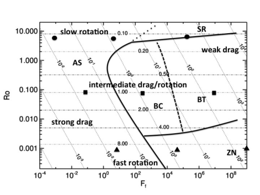
Figure 1:

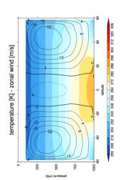
(a) $\mathcal{F}_{f}=1.5\times 10^{-3}$, $\mathcal{R}o=8$

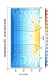
(b) $\mathcal{F}_{f}=1$, $\mathcal{R}o=8$

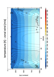
(c) $\mathcal{F}_{f}=4\times 10^{5}$, $\mathcal{R}o=8$

(d) $\mathcal{F}_{f}=10^{-1}$, $\mathcal{R}o=0.08$

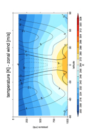
(e) $\mathcal{F}_{f}=10^{2}$, $\mathcal{R}o=0.08$

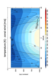
(f) $\mathcal{F}_{f}=4\times 10^{5}$, $\mathcal{R}o=0.08$

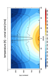
(g) $\mathcal{F}_{f}=10$, $\mathcal{R}o=10^{-3}$

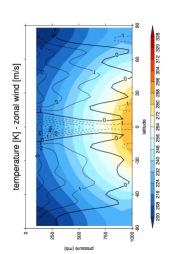
(h) $\mathcal{F}_{f}=10^{4}$, $\mathcal{R}o=10^{-3}$

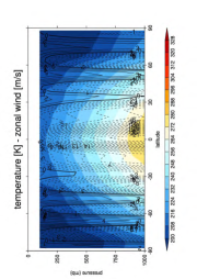
(i) $\mathcal{F}_{f}=10^{9}$, $\mathcal{R}o=10^{-3}$

Figure 2:

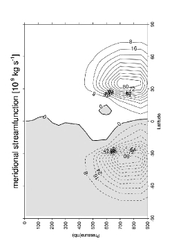
(a) $\mathcal{F}_{f}=1.5\times 10^{-3}$, $\mathcal{R}o=8$

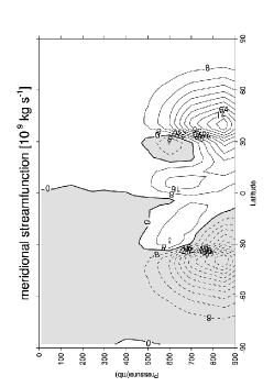
(b) $\mathcal{F}_{f}=1$, $\mathcal{R}o=8$

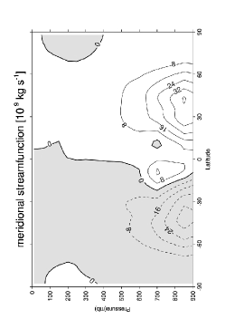
(c) $\mathcal{F}_{f}=4\times 10^{5}$, $\mathcal{R}o=8$

(d) $\mathcal{F}_{f}=10^{-1}$, $\mathcal{R}o=0.08$

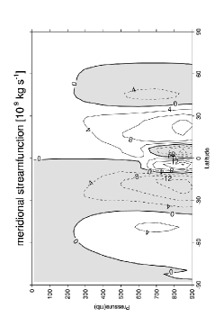
(e) $\mathcal{F}_{f}=10^{2}$, $\mathcal{R}o=0.08$

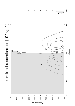
(f) $\mathcal{F}_{f}=4\times 10^{5}$, $\mathcal{R}o=0.08$

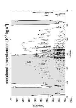
(g) $\mathcal{F}_{f}=10$, $\mathcal{R}o=10^{-3}$

(h) $\mathcal{F}_{f}=10^{4}$, $\mathcal{R}o=10^{-3}$

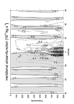
(i) $\mathcal{F}_{f}=10^{9}$, $\mathcal{R}o=10^{-3}$

Figure 3:

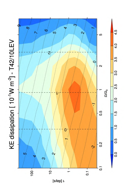
Figure 4:

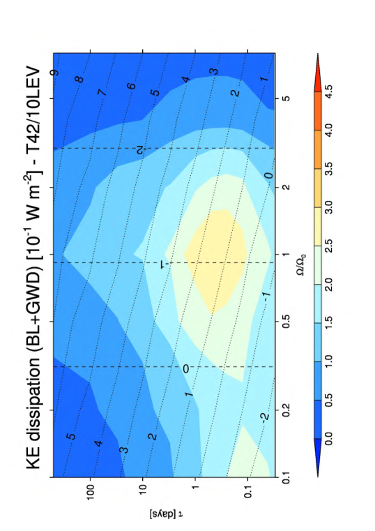
Figure 5:

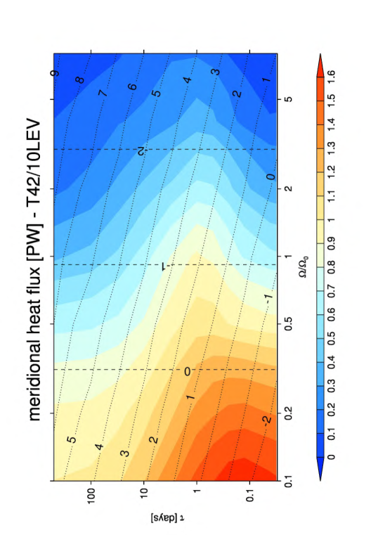
Figure 6:

Figure 7:

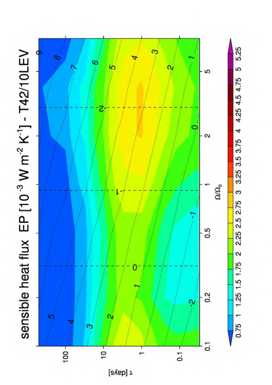
Figure 8:

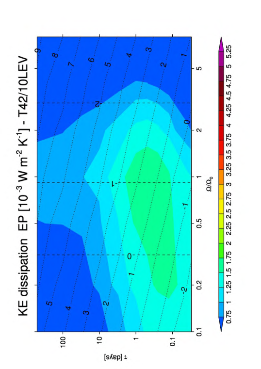
Figure 9:

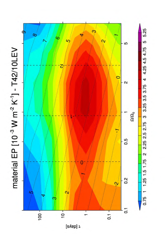
Figure 10:

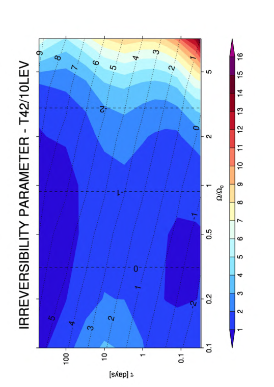
Figure 11:

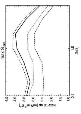
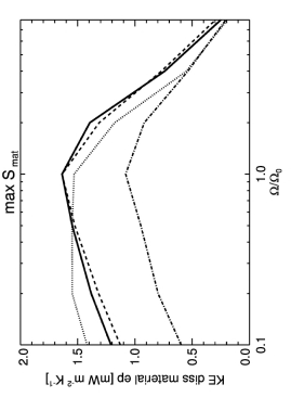
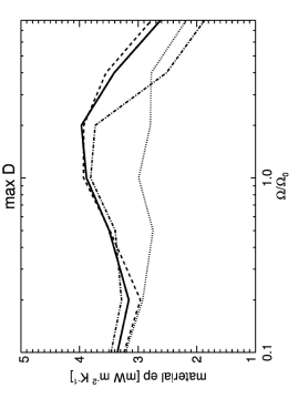
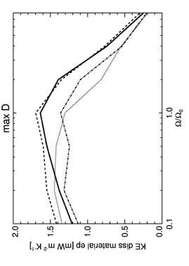
Figure 12:

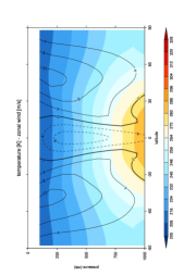
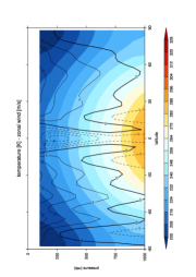
Figure 13:

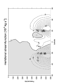
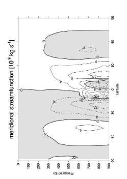
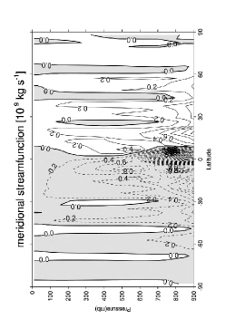
Figure 14:

References

- Burrows et al. (1997) Burrows, A. et al., 1997. A nongray theory of extrasolar giant planets and brown dwarfs. The Astrophysical Journal 491, 856–875.
- Arya (1988) Arya, S. P., 1988. Introduction to Micrometeorology. Accademic Press.
- Donohe and Battisti (2012) Donohoe, A. and Battisti D. S., 2012. What determines meridional heat transport in climate models? Journal of Climate 25, 3832 – 3850.
- Becker (2001) Becker, E., 2001. Symmetric stress tensor formulation of horizontal momentum diffusion in a global model of atmospheric circulation. Journal of Atmospheric Sciences 58, 269–282.
- Berger (1978) Berger, A., 1978. Long-term variations of daily insolation and quaternary climatic change. J. Atmos. Sci. 35, 2362-2367
- Bonfils and coauthors (2012) Bonfils, X. et al., 2012. The HARPS search for southern extra-solar planets XXXI. the m-dwarf sample. Astronomy and Astrophysics, in press.
- Borucki et al. (2011) Boruck, W. and coauthors, 2011. Characteristics of Planetary Candidates Observed by Kepler. II. Analysis of the First Four Months of Data The Astrophisical Journal 736, 19.
- Boschi et al. (2012) Boschi, R., Lucarini, V., Pascale, S., 2012. Bistability of the climate around the habitable zone: a thermodynamic investigation. http://arxiv.org/abs/1207.1254.
- Budyko (1969) Budyko, M. I., 1969. The effect of solar radiation variations on the climate of the Earth. Tellus 5, 611-619.
- Caballero et al. (2008) Caballero et al., 2008. Axisymmetric, nearly inviscid circulations in non-condensing radiative-convective atmospheres. Quarterly Journal of the Royal Meteorological Society 134, 1269–1285.
- Charbonneau et al. (2009) Charbonneau et al., 2009. A super-Earth transiting a nearby low-mass star. Nature 462, 891–894.
- Clancy et al. (2007) Clancy et al., 2007. Dynamics of the venus upper atmosphere: global-temporal distribution of winds, temperature, and CO at the Venus mesopause. Bull. Am. Astron. Soc. 39, 539.
- Dahms et al. (2012) Dahms, E., Lunkeit, F., Fraedrich, K., 2012. Low-frequency climate variability of an aquaplanet. J. Clim, submitted.
- DeGroot and Mazur (1984) DeGroot, S., Mazur, P., 1984. Non-equilibrium thermodynamics. Dover.
- Dewar (2005) Dewar, R. C., 2005. Maximum entropy production and the fluctuation theorem. Journal of Physics A 38, L371–L381.
- Dobbs-Dixon et al. (2012) Dobbs-Dixon, I., Agol, E., and Burrows, A., 2012. The Impact of Circumplantary Jets on Transit Spectra and Timing Offsets for Hot Jupiters. The Astrophisical Journal 751, 87
- Dvorak (2008) Dvorak, R., 2008. Extrasolar Planets. Wiley-VHC.
- Eady (1949) Eady, E., 1949. Long waves and cyclone waves. Tellus 1, 33–52.
- Egger (1999) Egger, J., 1999. Numerical generation of entropies. Monthly Weather Review 127, 2211–2216.
- Eliasen et al. (1970) Eliasen, E., Machenhauer, B., Rasmussen, E., 1970. On a numerical method for integration of the hydrodynamical equations with a spectral representation of the horizontal fields. Report no. 2, Inst. of Theor. Met., University of Copenhagen.
- Fermi (1956) Fermi, E., 1956. Thermodynamics. Dover.
- Fraedrich et al. (2005) Fraedrich, K., Jansen, H., Kirk, E., Luksch, U., Lunkeit, F., 2005. The planet simulator: towards a user friendly model. Meteorologische Zeitschrift 14 (3), 299–304.
- Fraedrich and Lunkeit (2008) Fraedrich, K., Lunkeit, F., 2008. Diagnosing the entropy budget of a climate model. Tellus A 60 (5), 921–931.
- Fraedrich et al. (2005) Fraedrich, K., E. Kirk, U. Luksch, and F. Lunkeit, 2005. The Portable University Model of the Atmosphere (PUMA): Storm track dynamics and low frequency variability. Meteorol. Zeitschrift 14, 735-745.
- Frierson et al. (2006) Frierson, D. M. W., Held I. M., Zurita-Gotor, P., 2006. A gray-radiation aquaplanet moist GCM. Part I: static stability and eddy scale. J. Atmos. Sci. 63, 2548–2566
- Gallavotti (2006) Gallavotti, G., 2006. Encyclopedia of mathematical physics. Elsevier, Ch. Nonequilibrium statistical mechanics (stationary): overview, pp. 530–539.
- Geisler et al. (1983) Geisler, J. E., Pitcher, E. J., Malone, R. C., 1983. Rotating-fluid experiments with an atmospheric general circulation model. Journal of Geophysical Research 88 (C14), 9706–9716.
- Genio and Suozzo (1987) Genio, A. D., Suozzo, R., 1987. A comparative study of rapidly and slowly rotating regimes in a terrestrial general circulation model. J. Atmos. Sci. 44, 973–986.
- Goody (2000) Goody, R., 2000. Sources and sinks of climate entropy. Quarterly Journal of the Royal Meteorological Society 126, 1953–1970.
- Goody (2007) Goody, R., 2007. Maximum entropy production in climate theory. Journal of the Atmospheric Sciences 64, 2735–2739.
- Grinstein and Linsker (2007) Grinstein, G., Linsker, R., 2007. Comments on a derivation and application of the maximum entropy production principle. J. Phys A 40, 9717–9720.
- Held and Hou (1980) Held, I. M., Hou, A. Y., 1980. Nonlinear axially symmetric circulations in a nearly inviscid atmosphere. Journal of Atmospheric Sciences 37, 515–533.
- Heng (2012) Heng, K., 2012. The study of climates of alien worlds. American Scientist 100 (4), 334–341, arXiv: 1206.3640
- Heng et al. (2011a) Heng, K., Frierson, D. M., Phillipps, P. J., 2011a. Atmospheric circulation of tidally locked exoplanets: II dual-band radiative transfer and convective adjustment. Monthly Notices of the Royal Astronomical Society 420, 2669–2696.
- Heng et al. (2011b) Heng, K., Menou, K., Phillips, P. J., 2011b. Atmospheric circulation of tidally locked exoplanets: a suite of benchmark tests for dynamical solvers. Monthly Notices of the Royal Astronomical Society 413, 2380–2402.
- Heng and Vogt (2011) Heng, K. and Vogt, S. S., 2011. Gliese 581g as a scaled-up version of Earth: atmospheric circulation simulations. Mon. Not. R. Astron. Soc. 415, 2145.
- Hide (1953) Hide, R., 1953. Some experiments on thermal convection in a rotating liquid. Q. J. R. Meteorol. Soc. 79, 161.
- Hide (1969) Hide, R., 1969. Some laboratory experiments on free thermal convection in a rotating fluid subject to a horizontal temperature gradient and their relation to the theory of the global atmosphric circulation. Corby, G.A. (Ed.), The Global Circulation of the Atmosphere, Royal Meteorological Society, London, 196–221.
- Hide (2010) Hide, R., 2010. A path of discovery in geophysics fluid dynamics. Astronomy and Geophysics 51 (4), 16–23.
- Hide and Mason (1975) Hide, R., Mason, P., 1975. Some experiments on thermal convection in a rotating liquid. Adv. Phys. 24, 47–99.
- Holton (2004) Holton, J., R., 2004. An introduction to Dynamic Meteorology. Elsevier Academic Press.
- Hourdin et al. (1995) Hourdin, F., O. et al. 1995. Numerical simulations of the general circulations of the atmosphere of Titan. Icarus 117, 358–374.
- Hunt (1979) Hunt, B., 1979. The influence of the earth’s rotation rate on the general circulation of the atmosphere. J. Atmos. Sci. 36, 1392–1408.
- Jablonowski and Williamson (2011) Jablonowski, C., Williamson, D., 2011. Numerical techniques for global atmospheric models. Springer, Ch. The pros and cons of diffusion, filters and fixers in atmospheric general circulation models, pp. 381–493.
- James (1994) James, I., 1994. Introduction to Circulating Atmosphere. Cambridge University Press.
- James and Gray (1986) James, I., Gray, L., 1986. Concerning the effect of surface drag on the circulation of a baroclinic planetary atmosphere. Quart. J. R. Met. Soc. 112, 1231–1250.
- James (1987) James, I. N., 1987. Suppression of baroclinic instability in horizontal sheared flows. Journal of Atmospheric Sciences 44 (24), 3710–3720.
- Johnson (1997) Johnson, D., 1997. ”General coldness of climate” and the second law: Implications for modelling the earth system. Journal of Climate 10, 2826–2846.
- Johnson (2000) Johnson, D. R., 2000. General Circulation Model Development: Past, Present and Future. Accademic Press, New York, Ch. Entropy, the Lorenz Energy Cycle and Climate, pp. 659–720.
- Joshi (2003) Joshi, M. M., 2003. Climate model studies of synchronously rotating planets Astrobiology 3(2), 415-27, PMID 14577888
- Jupp and Cox (2010) Jupp, T., Cox, P., 2010. MEP and planetary climates: insights from a two-box climate model containing atmospheric dynamics. Philosophical Transactions of the Royal Society B 365, 1355–1365.
- Kleidon (2009) Kleidon, A., 2009. Nonequilibrium thermodynamics and maximum entropy production in the earth system. Naturwissenschaften 96, 653–677.
- Kleidon et al. (2006) Kleidon, A., Fraedrich, K., Kirk, E., Lunkeit, F., 2006. Maximum entropy production and the strenght of boundary layer exchange in an atmospheric general circulation model. Geophysical Research Letters 33, doi:10.1029/2005GL025373.
- Kleidon et al. (2003) Kleidon, A., Fraedrich, K., Kunz, T., Lunkeit, F., 2003. The atmospheric circulation and the states of maximum entropy production. Geophysical Research Letters 30 (23), doi:10.1029/2003GL018363.
- Kleidon and Lorenz (2005) Kleidon, A., Lorenz, R., 2005. Non-equilibrium Thermodynamics and the Production of Entropy. Understanding Complex Systems. Springer, Berlin.
- Kondepudi and Prigogine (1998) Kondepudi, D., Prigogine, I., 1998. Modern Thermodynamics: From Heat Engines to Dissipative Structure. John Wiley, Hoboken, N.J.
- Kundu and Cohen (2004) Kundu, P., Cohen, I. M., 2004. Fluid Mechanics. Accademic Press.
- Kunz et al. (2008) Kunz, T., Fraedrich, K., Kirk, E., 2008. Optimisation of simplified GCMs using circulation indices and maximum entropy production. Climate Dynamics 30, 803–813.
- Kuo (1965) Kuo, H., 1965. On formation and intensification of tropical cyclones through latent heat release by cumulus convection. J. Atmos. Sci. 22, 40–63.
- Kuo (1974) Kuo, H., 1974. Further studies of the parametrisation of the influence of cumulus convection on large-scale flow. J. Atmos. Sci. 31, 1232–1240.
- Lacis and Hansen (1974) Lacis, A., Hansen, K., 1974. A parametrisation for the absorption of solar radiation in the earth’s atmosphere. J. Atmos. Sci. 31, 118–133.
- Laursen and Eliasen (1989) Laursen, L., Eliasen, E., 1989. On the effect of the damping mechanisms in an atmospheric general circulation model. Tellus 41A, 385–400.
- Lewis et al. (2010) Lewis N. K. et al., 2010. Atmospheric circulation of eccentric hot neptune GJ436b. The Astrophisical Journal 720, 344, doi:10.1088/0004-637X/720/1/344.
- Lorenz (1955) Lorenz, E., 1955. Available potential energy and the maintenance of the general circulation. Tellus 7, 271–281.
- Lorenz (1960) Lorenz, E., 1960. Generation of available potential energy and the intensity of the general circulation. Pergamon, Tarrytown, N.Y.
- Lorenz (1967) Lorenz, E., 1967. The nature and theory of the general circulation of the atmosphere. Vol. 218.TP.115. World Meteorological Organization.
- Lorenz et al. (2001) Lorenz, R., Lunine, J., Withers, P., McKay, C., 2001. Titan, Mars and Earth: Entropy production by latitudinal heat transport. Geophysical Research Letters 28 (3), 415–418.
- Louis (1979) Louis, J., 1979. A parametric model of vertical eddy fluxes in the atmosphere. Bound. Layer Meteorol., 187–202.
- Louis et al. (1981) Louis, J., Tiedke, M., Geleyn, J., 1981. A short history of the pbl parametrisation at ecmwf. Proceedings of the ECMWF Workshop on Planetary Boundary Layer Parametrization, 59–80.
- Lucarini (2009) Lucarini, V., 2009. Thermodynamic efficiency and entropy production in the climate system. Physical Review E 80, 021118, doi:10.1103/PhysRevE.80.02118.
- Lucarini (2012) Lucarini, V., 2012. Modelling complexity: the case of climate science. arXiv:1106.1265v1 [physics.hist-ph]; in press, Proceedings of the Conference ”Models, Simulation and the Reduction of Complexity”, De Gruyter Verlag, Hamburg.
- Lucarini and Ragone (2011) Lucarini, V., Ragone, F., 2011. Energetics of Climate Models: Net Energy Balance and Meridional Enthalpy Transport. Reviews of Geophysics 49, RG1001, doi:10.1029/2009RG000323.
- Lucarini et al. (2010) Lucarini, V., Fraedrich, K., Lunkeit, F., 2010. Thermodynamic analysis of snowball earth hysteresis experiment: efficiency, entropy production and irreversibility. Quarterly Journal of Royal Meteorological Society 136, 1–11.
- Lucarini et al. (2011) Lucarini, V., Fraedrich, K., Ragone, F., 2011. New results on the thermodynamic properties of the climate. Journal of the Atmospheric Sciences 68, 2438–2458.
- Lunkeit et al. (2010) Lunkeit, F., Borth, H., Böttinger, M., Fraedrich, K., Jansen, H., Kirk, E., Kleidon, A., Luksch, U., Paiewonsky, P., Schubert, S., Sielmann, S., Wan, H., 2010. Planet simulator, reference manual (version 16). Tech. rep., University of Hamburg, www.mi.uni-hamburg.de/Downloads-un.245.0.html.
- Menou and Rauscher (2009) Menou, K., Rauscher, E., 2009. Atmospheric circulations of hot jupiters: a shallow three dimensional model. The Astrophysical Journal 700, 887–897.
- Merlis and Schneider (2010) Merlis, T. M. and Schneider, T., 2010. Atmospheric dynamics of Earth-like tidally locked aquaplanets. Journal of Advances in Modeling Earth Systems, 2 (13), 17 pp.
- Miller et al. (2011) Miller L. M., Gans F., Kleidon A., 2011. Jet stream wind power as a renewable energy resource: little power, big impacts. Earth Syst. Dynam. 2, 201-212.
- Mitchell and Vallis (2010) Mitchell, J. L. and Vallis, G. K., 2010. The transition to superrotation in terrestrial atmospheres. Journal of Geophysical Research, 115 E12008, doi:10.1029/2010JE003587.
- Navarra and Boccaletti (2002) Navarra, A., Boccaletti, C., 2002. Numerical general circulation experiments of sensitivity to earth rotation rate. Climate Dynamics 19, 467–483.
- Orszag (1970) Orszag, S., 1970. Transform method for the calculation of vector coupled sums. J. Atmos. Sci., 890–895.
- Ozawa et al. (2003) Ozawa H, Ohmura A, Lorenz R. D., Pujol T., (2003). The second law of thermodynamics and the global climate system: A review of the maximum entropy production principle. Reviews of Geophysics 41 1018, 2003 (doi: 10.1029/2002RG000113)
- Paltridge (1975) Paltridge, G. W., 1975. Global dynamics and climate-a system of minimum entropy exchange. Quarterly Journal of the Royal Meteorological Society 101, 475–484.
- Paltridge (1978) Paltridge, G. W., 1978. The steady state format of global climate. Quarterly Journal of Royal Meteorological Society 104, 927–945.
- Paltridge (2001) Paltridge, G. W., 2001. A physical basis for a maximum of thermodynamic dissipation of the climate system. Quarterly Journal of the Royal Meteorological Society 127, 305–313.
- Paoletti et al. (1989) Paoletti, S., Rispoli, F., Sciubba, E., 1989. Calculation of exergetic losses in compact heat exchanger passages. ASME AES 10 (2), 21–29.
- Pascale et al. (2011a) Pascale, S., Gregory, J., Ambaum, M., Tailleux, R., 2011a. Climate entropy budget of the HadCM3 atmosphere-ocean general circulation model and FAMOUS, its low-resolution version. Climate Dynamics 36 (5-6), 1189–1206.
- Pascale et al. (2011b) Pascale, S., Gregory, J., Ambaum, M., Tailleux, R., 2011b. A parametric sensitivity study of entropy production and kinetic energy dissipation using the FAMOUS AOGCM. Climate Dynamics, doi 10.1007/s00382–011–0996–2.
- Pauluis and Held (2002a) Pauluis, O., Held, M., 2002a. Entropy budget of an atmosphere in radiative-convective equilibrium. Part I: Maximum work and frictional dissipation. Journal of the Atmospheric Sciences 59, 125–139.
- Pauluis and Held (2002b) Pauluis, O., Held, M., 2002b. Entropy budget of an atmosphere in radiative-convective equilibrium. Part II: Latent heat transport and moist processes. Journal of the Atmospheric Sciences 59, 140–149.
- Peixoto et al. (1991) Peixoto, J., Oort, A., de Almeida, M., Tomé, A., 1991. Entropy budget of the atmosphere. Journal of Geophysical Research 96, 10981–10988.
- Peixoto and Oort (1992) Peixoto, J. P., Oort, A., 1992. Physics of the Climate. Springer-Verlag, New York.
- Pierrehumbert (2010) Pierrehumbert, R. T., A Palette of Climates for Gliese 581g. The Astrophysical Journal Letters 726 (1), L8.
- Rauscher and Menou (2012) Rauscher E. and Menou, K., 2012. The role of drag in the energetics of strongly forced exoplanets. The Astrophisical Journal 745, 78 doi:10.1088/0004-637X/745/1/78
- Read (2001) Read, P., 2001. Transition to geostrophic turbulence in the laboratory, and as a paradigm in atmospheres. Surveys Geophys. 22, 231–249.
- Read (2011) Read, P., 2011. Dynamic and circulation regimes of terrestrial planets. Planetary and space sciences 59, 900–914.
- Read et al. (1998) Read, P., Collins, M., Früh, W.-G., Lewis, S., Lovegrove, A., 1998. Wave interactions and baroclinic chaos: a paradigm for long timescale variability in planetary atmospheres. Chaos Solitons Fractals 9, 1221–1227.
- Adams and Rennó (2005) Adams, D., K., Rennó, N., O., 2005. Thermodynamic efficiencies of an idealized global climate model. Climate Dynamics 25, 801–813.
- Rodgers (1976) Rodgers, C., 1976. Minimum entropy exchange principle-reply. Quarterly Journal of Royal Meteorological Society 102, 455–457.
- Sasamori (1968) Sasamori, T., 1968. The radiative cooling calculation for application to general circulation experiments. J. Appl. Meteorol. 7, 721–729.
- Schulman (1977) Schulman, L. L., 1977. A theoretical study of the efficiency of the general circulation, J. Atmos. Sci., 34, 559 580.
- Seager and Deming (2010) Seager, S. and Deming, D., 2010. Exoplanet atmospheres. Annual Review of Astronomy and Astrophysics. 48, 631–672.
- Sellers (1969) Sellers, W. D. 1969.A global climatic model based on the energy balance of the Earth-Atmosphere system. J. Appl. Meteor. 8, 392-400.
- Showman et al. (2010) Showman, A., Cho, J.-K., Menou, K., 2010. Atmospheric Circulation of Exoplanets. Invited review for the book ”Exoplanets”. S. Seager Eds., Univ. Arizona Press, pp 471-516.
- Showman et al. (2009) Showman, A. P., Fortney, J. J., Lian, Y., Marley, M. S., Freedman, R. S., Knutson, H. A., Charbonneau, D., 2009. Atmospheric circulation of hot jupiters: Coupled radiative-dynamical general circulation model simulations of HD 189733b and HD 209458b. The Astrophysical Journal 699, 564–584.
- Slingo and Slingo (1991) Slingo, A., Slingo, J., 1991. Response of the national center for atmospheric research community climate model to improvements in the representation of clouds. J. Geophys. Res. 96, 341–357.
- Stephens (1978) Stephens, G., 1978. Radiation profiles in extended water clouds. II: parametrization schemes. J. Atmos. Sci. 35, 2123–2132.
- Stephens et al. (1982) Stephens, G., Ackermann, S., Smith, E., 1982. A shortwave parametrization scheme. J. Atmos. Sci. 41, 687–690.
- Taylor (2010) Taylor, F., 2010. Planetary atmospheres. Oxford University Press.
- Thrastarson and Cho (2011) Thrastarson H. T. and Cho J. Y-K. (2011) Relaxation Time and Dissipation Interaction in Hot Planet Atmospheric Flow Simulations. The Astrophisical Journal 729, 117.
- Udry and Santos (2007) Udry, S., Santos, N. C., 2007. Statistical properties of exoplanets. Annual Review of Astronomy and Astrophysics 45, 397–439
- Valencia et al. (2007) Valencia, V., Sasselov, D. D., O’Connell, R., 2007. Radius and structure models of the first super-earth planet. The Astrophysical Journal 656 (1), 545–551.
- Vallis (2006) Vallis, G. K., 2006. Atmospheric and Oceanic Fluid Dynamics. Cambridge University Press.
- Vallis and Farneti (2009) Vallis, G. K., Farneti, R., 2009. Meridional energy transport in the coupled atmosphere-ocean system: scaling and numerical experiments. Quarterly Journal of Royal Meteorological Society 135, 1643–1660.
- Wang (2012) Wang, Y. and Read, P., 2012. Diversity of planetary atmospheric circulations and climates in a simplified general circulation model. Proceedings IAU Symposium No. 293, 2012
- Williams and Pollard (2002) Williams, D., Pollard, D., 2002. Earth-like worlds on eccentric orbits: excursions beyond the habitable zone. International Journal of Astrobiology 1 (1), 61–69.
- Williams and Pollard (2003) Williams, D., Pollard, D., 2003. Extraordinary climates of Earth-like planets: three-dimensional climate simulations at extreme obliquity. International Journal of Astrobiology 2 (1), 1–19.
- Williams (1988a) Williams, G., P., 1988a. The dynamical range of global circulations - I. Climate Dynamics 2, 205–260.
- Williams (1988b) Williams, G. P., 1988b. The dynamical range of global circulations - II. Climate Dynamics 3, 45–84.
- Williams (1978) Williams, G., P., 1978. Planetary circulation. I: Barotropic representation of jovian and terrestrial turbulence. J. Atmos. Sci. 35, 1399–1426.
- Woollings and Thuburn (2006) Woollings, T., Thuburn, J., 2006. Entropy sources in a dynamical core atmosphere model. Quarterly Journal of the Royal Meteorological Society 132, 43–59.
- Wordsworth et al. (2011) Wordsworth, R., Forget, F., Selsis, F., Millour, E., Charnay, B., Madeleine, J.-B., 2011. Gliese 581d is the First Discovered Terrestrial-mass Exoplanet in the Habitable Zone. The Astrophysical Journal Letters 733, Issue 2, doi: 10.1088/2041–8205/733/2/L48.
- Wordsworth et al. (2008) Wordsworth, R., Read, P., Yamazaki, Y., 2008. Turbulence, waves and jets in a differential heated rotating annulus experiment. Phys. Fluids 20, 126602, doi:10.1063/1.2990042.