The Australia Telescope Large Area Survey: Spectroscopic Catalogue and Radio Luminosity Functions

Abstract

The Australia Telescope Large Area Survey (ATLAS) has surveyed seven square degrees of sky around the Chandra Deep Field South (CDFS) and the European Large Area ISO Survey - South 1 (ELAIS-S1) fields at 1.4 GHz. ATLAS aims to reach a uniform sensitivity of $10\,\mu$Jy beam^-1 rms over the entire region with data release 1 currently reaching $\sim 30\,\mu$Jy beam^-1 rms. Here we present 466 new spectroscopic redshifts for radio sources in ATLAS as part of our optical follow-up program. Of the 466 radio sources with new spectroscopic redshifts, 142 have star-forming optical spectra, 282 show evidence for AGN in their optical spectra, 10 have stellar spectra and 32 have spectra revealing redshifts, but with insufficient features to classify. We compare our spectroscopic classifications with two mid-infrared diagnostics and find them to be in broad agreement. We also construct the radio luminosity function for star-forming galaxies to z $=0.5$ and for AGN to z $=0.8$. The radio luminosity function for star-forming galaxies appears to be in good agreement with previous studies. The radio luminosity function for AGN appears higher than previous studies of the local AGN radio luminosity function. We explore the possibility of evolution, cosmic variance and classification techniques affecting the AGN radio luminosity function. ATLAS is a pathfinder for the forthcoming EMU survey and the data presented in this paper will be used to guide EMU’s survey design and early science papers.

1 Introduction

Extragalactic radio sources comprise both star-forming (SF) galaxies and active galactic nuclei (AGN) (Condon 1992). In order to understand the history of the Universe we must unravel the cosmic evolution of both classes.

The galaxies that host radio sources display a range of different optical spectra. SF galaxy spectra are made up of direct emission from starlight and emission lines from Hii regions, and are quite easily identified at low redshifts. Some radio-loud AGN galaxies display strong high-excitation lines, either broad or narrow depending on obscuration and the orientation (Antonucci 1993), while others have weak or no emission features (e.g. Sadler et al. 2002). These spectral differences have been attributed to different accretion modes (Hardcastle, Evans, & Croston 2007; Croton et al. 2006). Sources without high-excitation lines are fuelled by the accretion of hot gas (‘hot mode’) while high-excitation sources require fuelling by cold gas (‘cold-mode’). The radiatively inefficient ‘hot-mode’ accretion is driven by the gravitational instability (Pope, Mendel, & Shabala 2012), and results in a geometrically thick, optically thin accretion disk within the hot broad-line region. On the other hand, the radiatively efficient ‘cold-mode’ accretion results in a geometrically thin, optically thick accretion disk within the broad-line region, and a narrow-line region further out. ‘Cold-mode’ accretion may be triggered by a merger event (e.g. Shabala et al. 2011), which can also trigger star-formation within the galaxy. Consequently, sources undergoing ‘cold-mode’ accretion may appear as ‘hybrid’ objects, that is, objects whose radio emission results from both star-formation and an AGN component (e.g. PRONGS, Mao et al. 2010b). Norris et al. (2011b) find that the extreme ULIRG, F00183-7111, is such an object.

Early radio surveys such as the 3C and 3CR Radio Surveys (Edge et al. 1959; Bennett 1962) had rms levels of a few Janskys and detected predominately powerful radio galaxies and quasars, allowing the cosmic history of these sources to be determined. Subsequent studies found that powerful radio galaxies and quasars evolve very strongly with redshift and the space density of these sources at z $\sim$ 2 is orders of magnitude higher than in the local Universe (e.g. Dunlop & Peacock 1990).

More recent wide-field radio surveys such as NVSS (Condon et al. 1998), SUMSS (Mauch et al. 2003) and FIRST (Becker, White, & Helfand 1995) have reached rms levels of a few mJy. At these flux densities the radio source population is dominated by radio galaxies and quasars powered by AGN (e.g. Sadler et al. 2002). The most powerful of these can be seen out to the edge of the visible Universe.

Source counts show a well-characterised upturn below 1 mJy beam^-1, which is above that predicted from the extrapolation of source counts for AGN with high-flux densities. Some studies attribute this to strong evolution of the SF galaxy luminosity function (e.g. Hopkins et al. 1998) while others find a significant contribution from lower-luminosity AGN (e.g. Huynh, Jackson, & Norris 2007). Sadler et al. (2007) found that low-luminosity AGN undergo significant cosmic evolution out to z = 0.7, consistent with studies of the optical luminosity function for AGN (e.g. Croom et al. 2004).

The deepest radio surveys now reach rms levels below 10 $\mu$Jy beam^-1 (e.g. Owen & Morrison 2008), but cover very small areas on the sky. The distribution of AGN and SF galaxies at low flux densities is not well known, with some studies finding the proportion of AGN declining with decreasing flux density and emission due to star-formation (SF) dominating (e.g. Mauch & Sadler 2007; Seymour et al. 2008), while other studies find the distribution is closer to a 50/50 split between SF galaxies and AGN down to $\sim$50 $\mu$Jy beam^-1 (e.g. Smolčić et al. 2008; Padovani et al. 2009). The lack of consensus of the distribution of AGN and SF at low flux densities is due to the small areas of sky surveyed at these sensitivities. Norris et al. (2011a) provide a brief comparison of the various studies and, in their figure 4, show that the fraction of SF galaxies at $<$100 $\mu$Jy beam^-1 could range from 30 - 80 per cent.

To date, understanding the evolution of the faint radio source population has been limited by the availability of sufficiently deep wide-area radio surveys. With the aim of imaging approximately seven square degrees of sky over two fields to 10 $\mu$Jy beam^-1 at 1.4 GHz, the Australia Telescope Large Area Survey (ATLAS, Norris et al. 2006; Middelberg et al. 2008) is the widest deep field radio survey yet attempted. ATLAS observes two separate fields so as to minimize cosmic variance (Moster et al. 2011): Chandra Deep Field South (CDFS) and European Large Area ISO Survey-South 1 (ELAIS-S1). The two fields were chosen to coincide with the Spitzer Wide-Area Infrared Extragalactic (SWIRE) Survey program (Lonsdale et al. 2003), so optical and mid-infrared identifications exist for most of the radio objects. CDFS also encompasses the Southern Great Observatories Origins Deep Survey (GOODS) field (Giavalisco et al. 2004).

The first data release (Data Release 1, or DR1) from ATLAS consists of the preliminary data published by Norris et al. (2006) and Middelberg et al. (2008) and reaches an rms sensitivity of $\sim$30$\,\mu$Jy beam^-1. The flux densities of DR1 are accurate to $\sim$10 per cent. The final ATLAS data release (DR3: Banfield et al., in preparation) will include additional data taken with the new CABB upgrade (Wilson et al. 2011) to the ATCA, and is expected to reach an rms sensitivity of $\sim$10$\,\mu$Jy beam^-1. For this paper we use radio data only from DR1.

Spectroscopic data provide accurate redshift information that can be used to determine absolute magnitudes, luminosities etc. This paper presents spectroscopic redshifts and spectroscopic classifications of radio sources in the ATLAS fields obtained using the AAOmega multi-fibre spectrograph at the Anglo-Australian Telescope (AAT) of sources in the ATLAS fields. Section 2 describes the observations and data analysis while Section 3 provides spectroscopic classifications and a description of the redshift catalogue. Section 4 discusses how the spectroscopic classifications compare to mid-infrared diagnostics and presents the radio luminosity function for ELAIS. Section 5 summarises our conclusions.

This paper uses H₀ = 70 km s^-1 Mpc^-1, $\Omega$_M = 0.3 and $\Omega$_Λ = 0.7 and the web-based calculator of Wright (2006) to estimate the physical parameters. Vega magnitudes are used throughout.

2 Observations and Data

2.1 Existing multi-wavelength data in ATLAS

Radio observations of ATLAS were carried out with the Australia Telescope Compact Array (ATCA, Project ID C1241). The ATCA was used in a variety of configurations (6A, 6B, 6C, 6D, 1.5D, 750A, 750B, 750D, EW367) to maximise $uv$ coverage. ATLAS observations were performed in mosaic mode with 40 pointings. The radio data used in this paper are from DR1 (Norris et al. 2006; Middelberg et al. 2008). CDFS was observed for 173 hours in total, or 8.2 hours per pointing with a resolution of $11^{\prime\prime}\times 5^{\prime\prime}$, and ELAIS was observed for 231 hours in total, or 10.5 hours per pointing with a resolution of $10.3^{\prime\prime}\times 7.2^{\prime\prime}$. There are 2018 radio sources in ATLAS within a total area of 7.65 square degrees. Smaller subsets of the ATLAS-CDFS field have been observed using the VLA by Kellermann et al. (2008) and Miller et al. (2008) at 1.4 GHz, but these data are not used here. Cross-matching of the ATLAS radio sources to optical and infrared counterparts is discussed by Norris et al. (2006) and Middelberg et al. (2008).

Infrared observations of ATLAS were obtained by SWIRE (Lonsdale et al. 2003), the largest Spitzer legacy program. SWIRE covers seven different fields including CDFS and ELAIS, totalling 60 - 65 square degrees in area at all seven Spitzer bands. SWIRE observes at 3.6, 4.5, 5.8, 8 and 24 $\mu$m down to 5–10 sigma detection limits (band-dependent) of 5, 9, 43, 40 and 193 $\mu$Jy respectively. The SWIRE data used in this paper are all from the third SWIRE data release.

2.2 Anglo-Australian Telescope Observations and Data Reduction

2.2.1 Source Selection

The aim of the optical observations was to obtain spectra for all radio sources. A small fraction ($<10\%$) have spectroscopic redshift information in the literature, predominately in CDFS. Consequently, these were assigned a low observation priority. Furthermore, radio sources with very faint or no optical counterparts were also assigned a low observation priority.

The position of counterparts for optical spectroscopy were identified with the SWIRE mid-infrared positions to provide sub-arcsecond astrometry (Norris et al. 2006; Middelberg et al. 2008). Optical photometry at these positions was derived from SWIRE (Lonsdale et al. 2003) to identify our sample in Table 1). The optical photometric data in SWIRE is not uniform, with areas where no data are available. Within these areas we used photometric data from SuperCOSMOS (Hambly et al. 2001).

The target sources were separated into ‘bright’, ‘intermediate’ and ‘faint’ sub-samples. The bright and intermediate sub-samples, with $R<20$ and $20<R<22$ respectively, were suitable for normal AAOmega observations. The ‘bright’ sample yielded the majority of the successfully determined redshifts presented in this paper. In addition, the ‘faint’ sample of sources with $R>22$ was selected for nod+shuffle observing, but these were unable to be completed because of poor weather. Of the 1120 sources observed in total, 692 were in the ‘bright’ sample, which yielded high quality redshifts for 466 sources.

2.2.2 Observation

Table 1: Summary of AAT observations. N. obs gives the number of fibres placed on science sources. The seeing information is from the AAT observing log. All observations were performed in multi-object mode with the exception of ‘CDFS A ns’ and ‘CDFS B ns’, which were performed in nod+shuffle mode. An unspecified Seeing value indicates an unavailable measurement.

Observation	N. obs.	Exposure (s)	Obs. date	Dichroic	Seeing (arcseconds)
CDFS A bright	329	3 $\times$ 1200	20071202	5700Å	2.4
CDFS A bright	343	4 $\times$ 1200	20071204	5700Å	…
CDFS B bright	329	4 $\times$ 1200	20071204	5700Å	…
CDFS A intermediate	343	4 $\times$ 1800	20071207	5700Å	1.9-2.5
CDFS B intermediate	329	2 $\times$ 1200	20071205	5700Å	1.8-2.3
CDFS A ns	162	1 $\times$ 1500	20071206	5700Å	1.4
CDFS A ns	162	13 $\times$ 2400	20071206,07,08	5700Å	1.2-3
CDFS A ns	187	5 $\times$ 2400	20071208	5700Å	1.2 - 1.7
CDFS B ns	187	1 $\times$ 1500	20071205	5700Å	2.3
CDFS A 2010	329	6 $\times$ 2400	20101206	5700Å	…
CDFS B 2010	329	2100+1500	20101207	5700Å	…
ELAIS bright	343	7 $\times$ 1200	20071205	5700Å	1.8
ELAIS bright	343	4 $\times$ 1800	20081221,22	6700Å	1.6-1.7
ELAIS bright	329	4 $\times$ 1800	20081224,25,26	6700Å	1.6-2.4
ELAIS 2010	343	1270+1770	20101208	5700Å	1.4 - 1.6

We obtained AAOmega observations of the ATLAS radio sources from December 1 to December 8, 2007 and December 20 to December 27, 2008, all of which were dark nights. AAOmega is the multi-object spectrograph on the Anglo-Australian Telescope (AAT). We also obtained some observations for ATLAS sources from December 1 to December 8, 2010 as part of a complementary project. The AAOmega spectrograph was used in multi-object mode (Saunders et al. 2004; Sharp et al. 2006) and nod+shuffle mode (Glazebrook & Bland-Hawthorn 2001). While the sensitive principle component analysis (PCA) based approach for deep observations with AAOmega (Sharp & Parkinson 2010) would likely have resulted in enhanced sensitivity, the technique was still under development at the time of our observations. We used the dual beam system with the 580V and 385R Volume Phase Holographic gratings. The 2007 and 2010 observations used the 5700Å dichroic beam splitter and covered the spectral range between 3700Å and 8500Å at central resolutions in each arm of R$\sim$1300 per 3.4 pixel spectral resolution element. The 2008 observations used the 6700Å dichroic beam splitter and covered the spectral range between 4700Å and 9500Å, which allows detection of H$\alpha$ to z $\sim$ 0.4.

Each of the three observing sessions over three years was compromised by poor weather, with only $16.9\%$ of scheduled time able to be used, severely restricting the sensitivity of the observations. The seeing ranged from 1.2^′′ to 3.0^′′. The observations are summarised in Table 1.

The sensitivity limit (SNR$=\sim$3 per-pixel) with AAOmega for our estimated exposure times was $R\sim 22$. The surface density of ATLAS sources at this sensitivity limit is $\sim$100/deg², with this value decreasing markedly for brighter sensitivity limits. Optimising the placement of the fibres still resulted in ‘spare fibres’ that could not be placed on ATLAS radio sources. The remaining fibres were allocated to three ATLAS related projects: the detection of a cluster associated with a wide-angle-tail galaxy, a sample of luminous red galaxies and a large sample of 24 $\mu$m excess sources in the ATLAS fields. The redshifts obtained for the cluster work have been published in Mao et al. (2010a) and the 24 $\mu$m data are presented in Appendix A and will be discussed in further detail in Norris et al. (in preparation), but are not discussed further in the context of this work.

2.2.3 Data Reduction

The spectroscopic data were processed using the 2dfDR software provided by the AAO. Source redshifts were determined using the runz redshift-fitting package using template cross-correlation or emission line fitting with a redshift quality flag out of 5 assigned via visual inspection of the fit. Spectra with a quality flag of 2 or below were discarded.

621 ATLAS radio sources were observed in ELAIS, with spectra of quality $>2$ obtained for 306 sources. 499 ATLAS radio sources were observed in CDFS, with spectra of quality $>2$ obtained for 160 sources. A total of 1120 ATLAS radio sources were observed, with spectra obtained for 466 sources yielding reliable redshifts from the AAOmega observations.

Our observations achieve $\sim 70\%$ completeness at $R\sim 20$ (Figure 1). This corresponds to the ability to detect typical SF galaxies to z $\sim 0.4$ and typical early-type galaxies to z $\sim 0.5$.

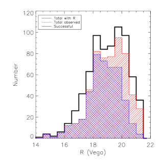
Figure 1: Histogram of $R$-band magnitudes for the target sources. The black histogram represents all ATLAS radio sources that have $R$-band magnitudes from SuperCOSMOS (Hambly et al. 2001), the red histogram represents the sources that were observed with AAOmega and the blue histogram represents all sources that had quality $>2$ spectra.

3 Results

3.1 Spectroscopic Classifications

In the course of measuring the redshift, each spectrum was inspected visually to determine whether the dominant physical process responsible for the radio emission was star-formation (SF) or an AGN. This method is similar to that used by previous studies (e.g Sadler et al. 2002). Sadler et al. (1999) reported that visual classifications can be used with confidence to analyse spectra from 2dF, the precursor to AAOmega.

SF galaxy spectra are typically dominated by strong, narrow emission lines including the Balmer series. We classified these spectra as ‘SF’. AGN, on the other hand, can have pure absorption-line spectra (‘E’), absorption-line spectra with some low-ionisation emission lines such as [OII] (3726 Å, 3729 Å) (‘E+OII’), emission-line spectra whose line ratios are indicative of AGN activity (‘AGNa’) and broad-line spectra (‘AGNb’). Figure 2 provides examples of each type of spectrum. Ten sources had stellar spectra and, upon visual inspection of the field, we attribute this to chance alignments and discard these data from further analysis in this work.

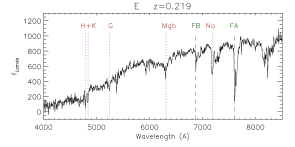
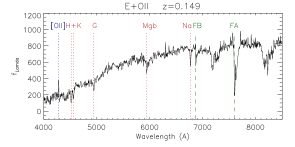
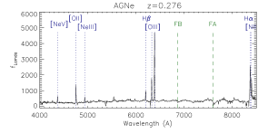
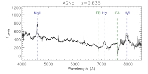
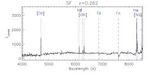
Figure 2: Examples of each spectroscopic classification. From top left the spectra are ‘E’, ‘E+OII’, ‘AGNe’, ‘AGNb’ and ‘SF’. The red dotted lines indicate prominent absorption features and the blue dotted lines indicate prominent emission features. The green dashed lines indicate the Fraunhofer A+B atmospheric absorption bands from O₂.

There are 142 SF, 282 AGN (110 E, 60 E+OII, 79 AGNe, 32 AGNb), 10 stars and 32 ‘unknown’ spectra that we are unable to spectroscopically classify, despite sufficient features for a redshift to be determined. The spectra that are classified as ‘unknown’ are typically at z $>$ 0.4, so H$\alpha$ is redshifted out of the spectrum. Furthermore, a ratio of [OIII]/H$\beta$ $\sim$ 1 could either indicate SF or AGN, and without further information spectroscopic classifications cannot be made. We acknowledge the presence of hybrid systems in our sample, but do not make any attempt to classify such sources in this paper and defer this to a future paper.

3.2 Redshift and Spectroscopic Classification Catalogue

The catalogue of redshifts and spectroscopic classifications is available as supplementary material in the online version of this paper. Table 2 provides the first ten lines of the catalogue.

Table 2: First 10 lines of the catalogue of new spectrosopic redshifts and spectroscopic classifications of the 466 radio-selected galaxies in ATLAS. Column 1 gives the ‘SID’ from Norris et al. (2006); Middelberg et al. (2008) and Columns 2 and 3 provide the position of the optical counterpart. The radio flux densities in Column 6 are from Norris et al. (2006); Middelberg et al. (2008) and are uncorrected for effects such as bandwidth smearing. Columns 5 and 6 give the SuperCOSMOS $R$ and $B$-band magnitudes (Hambly et al. 2001). Columns 7 and 8 present the spectroscopic redshifts and spectroscopic classifications determined in this paper and Columns 9 and 10 present the absolute $R$-band magnitude and 1.4 GHz radio luminosity.

SID	RA	Dec	S20	$R$	$B$	z	Spec. class.	MR	log L${}_{1.4\,GHz}$
	(J2000)	(J2000)	(mJy)	(Vega)	(Vega)				(W Hz-1)
S007	03:26:15.42	-28:46:30.80	0.71	20.19	22.52	0.7108	E+OII	-23.68	24.15
S009	03:26:16.32	-28:00:14.72	1.66	20.46	…	0.5295	E+OII	…	24.22
S012	03:26:22.06	-27:43:24.53	27.81	19.12	19.37	1.3871	AGNb	-25.01	26.42
S014	03:26:26.90	-27:56:11.65	4.14	17.98	18.92	0.8106	AGNb	-25.46	25.05
S015	03:26:29.13	-28:06:50.80	0.31	16.66	17.21	0.0579	SF	-20.44	21.40
S021	03:26:30.65	-28:36:58.03	1.86	18.98	21.54	0.4731	E	-23.89	24.15
S031	03:26:39.12	-28:08: 1.57	42.29	16.89	18.43	0.2184	E	-23.55	24.75
S037	03:26:43.38	-28:13:28.06	0.50	17.93	19.79	0.2956	SF	-23.39	23.12
S038	03:26:43.34	-28:22:11.43	8.28	19.37	21.69	0.3220	AGNe	-22.32	24.42
S042	03:26:48.47	-27:49:38.06	5.00	…	…	2.9869	AGNb	…	26.43

Figure 3 shows the redshift distribution of the 466 sources in ATLAS for which we obtained redshifts from AAOmega. The median redshift for the entire sample is 0.316 while the median redshift for CDFS is 0.332 and the median redshift for ELAIS is 0.315. The redshift peak in the CDFS redshift histogram at 0.6 $<$ z $<$ 0.7 corresponds to a known cosmic sheet (e.g. Norris et al. 2006). There is also a redshift peak in the ELAIS redshift histogram at $0.2<$ z $<0.4$. Mao et al. (2010a) discovered an overdensity in ELAIS at z $\sim 0.22$, associated with a large wide-angle tail galaxy (WAT). They also found an additional three WATs in ELAIS at $0.3<$ z $<0.4$, each of which is likely to be associated with a cluster of galaxies.

The most distant radio source in our observed sample is SWIRE3 J032648.47-274938.0 at a redshift of z = 2.99, and has been spectroscopically confirmed as a broad-line quasar with a radio power of 2.8 $\times$ 10²⁶ W Hz^-1.

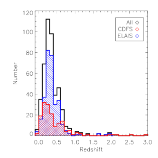
Figure 3: Histogram of spectroscopic redshifts in ATLAS. The red line shows data for CDFS and the blue line shows data for ELAIS. The black line is the total. The bins are 0.1 z wide.

We calculate the radio luminosity for each source with spectroscopic redshift information using

$${\rm L}_{\nu}=\frac{4\pi{\rm D}_{L}^{2}{\rm S}_{\nu obs}}{(1+z)^{1+\alpha}}$$ (1)

where L_ν is the luminosity in W Hz^-1 at the frequency $\nu$, D_L is the luminosity distance in metres, S_νobs is the observed flux density at the observing frequency, and $\alpha$ is the spectral index where spectral index is defined as S $\propto$ $\nu^{\alpha}$. We assume $\alpha$ = -0.75, which is a typical mean value for the synchrotron emission observed from faint radio sources (Ibar et al. 2010), both star-forming and AGN.

Figure 4 presents the luminosity histogram for sources with redshift information. The median L${}_{1.4\,\rm GHz}$ for these sources is $\sim 10^{23.1}$ W Hz^-1 with the SF source median L${}_{1.4\,\rm GHz}\sim 10^{22.6}$ W Hz^-1 and the AGN median L${}_{1.4\,\rm GHz}\sim 10^{23.4}$ W Hz^-1. The large overlap between the radio luminosity ranges for SF and AGN sources makes it impossible to determine whether sources with the ‘unknown’ spectroscopic classification are SF or AGN from this information alone.

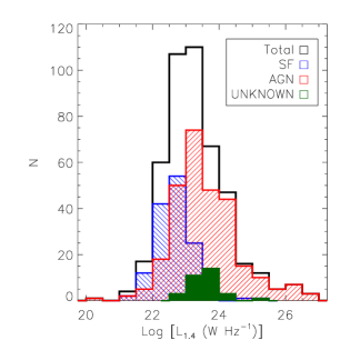
Figure 4: Radio luminosity histogram for our sample. Sources spectroscopically classified as SF are shown in blue, while those classified as AGN are shown in red. Those without spectroscopic classifications are shown in green.

4 Discussion

4.1 Mid-IR colours

We compare our spectroscopic classifications with those determined from mid-infrared colour-colour diagrams similar to those of Lacy et al. (2004) using the SWIRE data from Spitzer. Not all of the 466 sources with spectroscopic classifications have infrared data at the SWIRE wavelengths and, as such, comparisons may only be made where data is available at all wavelengths.

Figure 5 shows the $[3.6\,\mu\rm m]-[4.5\,\mu\rm m]$ against $[3.6\,\mu\rm m]-[8\,\mu$m] plot, where $[1]-[2]=-2.5$log(S₁/S₂), that is, the SWIRE colours are given in AB magnitude units to allow direct comparison with Richards et al. (2006). The spectroscopic classifications are plotted in different colours. The demarcation between AGN and SF galaxies is as expected (e.g Sajina, Lacy, & Scott 2005), which provides an independent validation of our visual spectroscopic classification method.

Richards et al. (2006) suggest that Type 1 quasars may be selected by taking $[3.6]-[4.5]>-0.1$. We apply this selection to our data and find 127 sources would be classified as Type 1 AGN (Figure 5). Of these 127 sources, we had spectroscopically classfied 55 as SF, 67 as AGN (27 AGNb, 36 AGNe, 4 E or E+OII) and 5 were ‘unknown’. While this method appears to select against E type sources more robustly than the Lacy et al. (2004) method below, the contamination by SF sources is considerable.

Lacy et al. (2004) imposed a MIR colour selection to select AGN in their sample of SDSS sources in the First Look Survey. Applying this selection criteria to the ATLAS data we classify 100 sources as AGN (Figure 6). Of the 100 AGN that satisfied the ‘Lacy’ AGN criteria, we had spectroscopically classified 18 as SF, 65 as AGN (26 AGNb, 27 AGNe, 12 E or E+OII) and 17 were ‘unknown’. Our spectroscopic classifications show that there is a significant region of overlap between SF and AGN sources on this MIR colour-colour plot. Indeed, the majority of the ‘unknown’ spectroscopic classifications fall in this region of overlap. A more stringent ‘diagonal boundary’ on the AGN selection may be better for AGN selection, but this would also lose many AGN in the overlap region. We note that Lacy et al. (2007) shifted the vertical boundary of the ‘Lacy’ wedge slightly but this does not affect our result significantly.

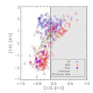
Figure 5: MIR $[3.6\,\mu\rm m]-[4.5\,\mu$m] vs. $[3.6\,\mu\rm m]-[8\,\mu$m] colour-colour plot. The data in blue show the sources classified spectroscopically as SF and those in red show the sources classified as AGN. Stars are shown in purple and the sources we were unable to classify spectroscopically are shown in green. The grey shaded region shows the location of the Richards et al. (2006) selection for Type 1 quasars.

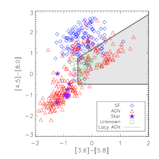
Figure 6: MIR $[3.6\,\mu\rm m]-[5.8\,\mu$m] vs. $[4.5\,\mu\rm m]-[8\,\mu$m] colour-colour plot. The data in blue show the sources classified spectroscopically as SF and those in red show the sources classified as AGN. Stars are shown in purple and the sources we were unable to classify spectroscopically are shown in green. The grey shaded region shows the location of the Lacy et al. (2004) selection for AGN.

Stern et al. (2005) used Spitzer data from the AGN and Galaxy Evolution Survey (AGES) to identify Type 1 AGN and we find their selection method to be a more robust way of identifying broad-line AGNs. Of the 48 sources that satisfy the “Stern Wedge”, only 6 had been spectroscopically classified as SF with the remaining 42 AGN comprising 25 “AGNb”, 12 “AGNe”, 3 “E” or “E+OII” and two “UNKNOWN” (Figure 7).

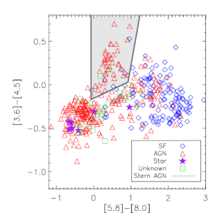
Figure 7: MIR $[5.8\,\mu\rm m]-[8\,\mu$m] vs. $[3.6\,\mu\rm m]-[4.5\,\mu$m] colour-colour plot. The data in blue show the sources classified spectroscopically as SF and those in red show the sources classified as AGN. Stars are shown in purple and the sources we were unable to classify spectroscopically are shown in green. The grey shaded region shows the location of the Stern et al. (2005) selection for AGN.

4.2 Mid-infrared Radio Correlation

Norris et al. (2006) and Middelberg et al. (2008) both use the Mid-Infrared Radio Correlation (MRC) to discriminate AGN from SF galaxies with ${\rm q}_{24}=\rm log(S_{24\mu\rm m}$/S${}_{1.4\rm GHz})\leq-0.16$ identified as AGN. This criterion ensures that sources have a ten-fold excess of radio emission over the MRC and are thus very likely AGN. We apply this discriminant and find 16 of the 466 sources satisfy this AGN criterion. The MRC using 24$\,\mu$m data is plotted against redshift in Figure 8.

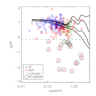
Figure 8: The mid-infrared radio ratio, q₂₄, against redshift. The data in blue show the sources that were classified spectroscopically as SF and those in red show the sources that were classified as AGN. The sources which we were unable to classify spectroscopically are shown in green. The black lines are expected q₂₄ tracks derived from SED templates for galaxies with total infrared luminosities of 10⁹ (normal galaxies), 10¹¹, 10¹² and 10${}^{13}L_{\odot}$ (ULIRGs) going from bottom to top, from Chary & Elbaz (2001). Sources with q₂₄ $\leq-0.16$ are shown in black and the dotted line is at q${}_{24}=-0.16$.

Only one source presents a conflict between the spectroscopic classification and that based on q₂₄. The source, S385 in CDFS, is spectroscopically classified as a SF galaxy, and lies close to the selection boundary but, at z = 0.6, it is difficult to assign a spectroscopic classification due to the dearth of strong optical features in the observed spectroscopic range.

The IR colours and the MRC in this paper are primarily used to determine the validity of the spectroscopic classifications that we presented in Section 3.1. We hereby conclude that our spectroscopic classifications are broadly reliable and for the remainder of this paper we will use the spectroscopic classifications only. The 32 sources that we were unable to classify spectroscopically as SF or AGN could not be unambiguously classified using the mid-infrared diagnostics.

We defer a more detailed exploration of classification limitations and ambiguities to a future paper that shall also utilise 843 MHz and 2.3 GHz ATLAS radio data from Randall et al. (2012) and Zinn et al. (in preparation). We also note the strength of classification techniques such as the k-Nearest Neigbour (kNN) classifier, which can operate on multi-dimensional datasets (e.g. Gieseke et al. 2011).

4.3 Computing the Radio Luminosity Function

The radio luminosity function (RLF) allows direct insight into the evolutionary history of galaxies. SF galaxies are known to positively evolve with redshift, that is, the radio luminosity and number density of SF galaxies is greater at higher redshifts (Hopkins et al. 1998; Afonso et al. 2005, Dwelly et al., in preparation). The evolution of powerful radio AGN is well understood with powerful radio AGN also evolving positively with redshift. The evolution of low-luminosity radio AGN is less well understood with some studies finding no evidence for any evolution of the RLF for low-luminosity radio AGN (e.g. Clewley & Jarvis 2004) and others finding that low-luminosity AGN do evolve with redshift, albeit more slowly than their high-luminosity counterparts (e.g Smolčić et al. 2009; McAlpine & Jarvis 2011). Deep radio data are being used to study low-luminosity AGN (e.g Kimball et al. 2011; Padovani et al. 2011). Best & Heckman (2012) suggest that the luminosity dependence of the evolution of the AGN RLF may be attributed to the varying fractions of ‘hot’ and ‘cold’ mode sources with redshift.

In order to calculate luminosity functions, the sample must have known redshifts as well as both an optical magnitude limit and a radio flux density limit (Schmidt 1968, 1977). Moreover, the sample volume must be large enough to mitigate the effects of cosmic variance (Moster et al. 2011). It is imperative that any incompleteness in the dataset is well understood.

4.3.1 RLF Survey Area

The ATLAS radio data cover $\sim 7.5$ square degrees on the sky, 2.96 square degrees in CDFS and 4.69 square degrees in ELAIS. AAOmega observations of ATLAS comprised two overlapping pointings in CDFS and a single pointing in ELAIS. The total area covered by AAOmega in CDFS is 2.83 square degrees and the total area covered by AAOmega in ELAIS is $\pi$ square degrees. The discrepancies in size and coverage are due to CDFS’s shape and the AAOmega observations actually extended beyond the boundary of the radio observations, whereas in ELAIS the AAOmega pointing was within the radio observations. For the construction of the RLF, the survey area must be limited to where there is data at both radio and optical bands.

Due to the presence of a strong ($>1$ Jy) source near the centre of the CDFS field (Norris et al. 2006) the CDFS radio image contains a number of artefacts. More advanced data reduction techniques have been applied to DR2 and DR3 and the CDFS radio image from these data releases is less affected by artefacts and has a more uniform rms. Due to the varying rms of the DR1 CDFS radio image, the remainder of this Section will deal only with ELAIS. The RLF for CDFS will be deferred to the release of DR2 and DR3.

The AAT observations for ELAIS cover only a single pointing so we limit the total area with which we can construct the RLF to $\pi$ square degrees, the field-of-view (FOV) of AAOmega.

4.3.2 The Radio Data

ATLAS DR1 is nominally quoted as having an rms of 30 $\mu$Jy beam^-1, but the sensitivity of the radio images is not uniform, typically being less sensitive closer to the edges. Figures 9 and 10 shows the varying rms in ELAIS at each radio source position. These values were calculated by producing an rms map and calculating the mean rms in the 75 $\times$ 75 pixels ($\sim$15 $\times$ 15 synthesised beams) surrounding the source position. To mitigate the effect of outlier pixels the brightest and faintest pixel in the rms grid were discarded when calculating the mean rms.

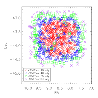
Figure 9: ELAIS’s rms characteristics, with four different rms bins chosen, and colour-coded.

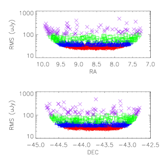
Figure 10: RMS against both RA and Dec for ELAIS with the same symbol scheme as above.

In order to construct the radio luminosity function we must calculate the maximum volume to which a source of a given radio luminosity may be detected (V_MAX). If the radio image had uniform sensitivity,

$$\rm V_{MAX} = \frac{4}{3}\pi\Omega\rm D_{MMAX}^{3}$$ (2)

where $\Omega$ is the solid angle (in steradians) subtended by the image, and D_MMAX is the maximum comoving distance in Mpc for a source of a given radio luminosity (Hogg 1999).

In order to account for the non-uniform sensitivity however, we must treat the radio image as a number of nested subimages, each with its own limiting flux density. Consequently, each subimage may be approximated by a uniform radio image, and sources that fall below $5\times$ rms (Figure 9) are discarded. For a sample with regions that have different sensitivies, the maximum volume available to each source may be calculated using the method described in section IIc of Avni & Bahcall (1980).

Using the Miriad task imhist we are able to calculate the total area of the radio image above each chosen flux limit. Consequently, for each source we are able to calculate the total volume available to the source, as well as the actual volume enclosed by that source using the method of Avni & Bahcall (1980). The calculations for V_enclosed and V_available are shown in Appendix B.

4.3.3 The Optical Data

We use the SuperCOSMOS (Hambly et al. 2001) optical magnitude data, which is limited at $B_{j}$ $\sim$ 23 and $R\sim$ 22. Sources fainter than these limits are discarded. Although deeper photometry exist within parts of the ATLAS fields (e.g., Lonsdale et al. 2003), SuperCOSMOS is the only survey to date that covers our region of interest uniformly. Moreover, the faintest sources observed successfully in our spectroscopic observations using the AAT have $R\sim 22$. Optical $k$-corrections were applied using the method from De Propris et al. (2004). Because both $R$ and $B$ band magnitudes are necessary to calculate the $k$-correction when calculating absolute magnitudes, we must determine magnitude limits for our spectroscopic observations for both photometric bands.

Figure 11 shows the completeness functions for both bands. We choose $R_{lim}$=20 and $B_{lim}$=22.5. There is still some incompleteness ($\sim$30 per cent) at these magnitude limits, but we choose these limits to maximise the number of sources that we can use to calculate the luminosity function. There is an additional incompleteness that we must account for (top panels of Figure 11) due to the fraction of sources that were not observed with the AAT. This is, in part, due to the poor observing conditions. In order to observe a dense field of sources completely it is often necessary to observe a number of fibre configurations and the poor observing conditions limited our ability to observe multiple configurations. We also selected against bright sources ($R<18$) because the magnitude range for any single observation is limited to $\sim$2 magnitudes to avoid the problem of scattered light. To account for these completeness issues, we take the product of these two corrections (C_i) and weight each source of a given magnitude by this correction when calculating the RLF (below). We can now calculate the maximum volume out to which the optical source could be detected. As two optical bands are necessary for $k$-correcting this dataset, we calculate V_MAX at both bands and take the smaller of the two to be the limiting value. The maximum volume to which the optical source can be detected may be calulated using Equation 2.

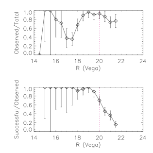
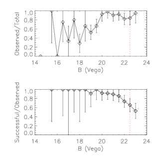
Figure 11: The top panels shows the fraction of sources observed against optical magnitude (left: $R$-band, right: $B$-band) within the FOV and the bottom panel shows the fraction of sources whose observations yielded quality spectra. The pink dotted lines indicate the magnitude limits. The error bars are Poisson. The error bars at bright magnitudes are large due to the small numbers in each bin.

4.3.4 V/V_MAX test

All sources fainter than the radio flux density and optical magnitude limits for our dataset have now been discarded. We remove any sources with stellar spectra as these are believed to be chance alignments, leaving a total of 226 sources in ELAIS out of the original 306 with which to calculate the radio luminosity function. Perhaps unsurprisingly, 71 per cent (17/24) of the ‘unknown’ spectroscopic-type sources were discarded due to their faint optical magnitudes. We do not account for the ‘unknown’ spectra for the remainder of this section. Although they will undoubtedly affect either or both the SF or the AGN RLF, there are only seven of these sources in our sample and their inclusion would not significantly change any of our results.

We can now check the completeness of our dataset using the V/V_MAX test of Schmidt (1968, 1977). We calculated both the available and enclosed volumes for each radio source, as well as both the volume and maximum volume out to which the optical source might be detected. We compare the maximum volume out to which the optical source may be detected (Equation 2) with the maximum volume available to each radio source (Equation 7) and take the smaller of the two as the limiting value, as in Equation 3.

$$\rm V_{MAX} = {\rm min}[\rm V_{(\rm MAX,OPT)},V_{(\rm available,RAD)}]$$ (3)

where V_MAX,OPT is the maximum volume to which the optical source may be detected, and V_{available,RAD} is the maximum volume available to the radio source.

Of the 226 radio sources in ELAIS with which we are able to construct the RLF, 146 (65 per cent) are detection-limited by the radio flux density limits. The detection of sources with radio luminosities greater than 10²⁴ W Hz^-1 is almost entirely governed by the optical magnitude limits. There is no discernable difference in the detection limit between SF and AGN. We calculate $\langle$V/V${}_{\rm MAX}\rangle$ to be 0.563 $\pm$ 0.011, which is consistent with positive evolution as $\langle$V/V${}_{\rm MAX}\rangle>0.5$.

The radio luminosity function for our sources was calculated using

$$\Phi=\displaystyle\sum\limits_{i=0}^{n}\frac{1}{{\rm V}_{{\rm MAX},i}}\pm\sqrt{\displaystyle\sum\limits_{i=0}^{n}\frac{1}{({\rm V}_{{\rm MAX},i})^{2}}}$$ (4)

where $\Phi$ is the density of sources in Mpc^-3dex^-1, $n$ is the number of sources, and V_MAX is the maximum volume out to which we can see the source.

To correct for incompleteness, we apply the corrections from Figure 11. The optical band that limits V_MAX is used to determine which completeness correction is used.

$$\Phi=\displaystyle\sum\limits_{i=0}^{n}\frac{1}{{\rm C}_{i}\times{\rm V}_{{\rm MAX},i}}\pm\displaystyle\sum\limits_{i=0}^{n}\frac{1}{\sqrt{(}\Delta{\rm V}_{{\rm MAX},i}^{2}+\Delta{\rm C}_{i}^{2})}$$ (5)

where C_i is from the completeness functions (Figure 11). Where the number of sources is small ($n<40$), the standard $\sqrt{n}$ approximation to Poisson errors are inaccurate, so for $n<40$ we have evaluated the 1-sigma Poisson errors using Gehrels (1986).

4.4 The RLF for ELAIS

Figure 12 and Table 3 show the resulting RLF over our entire redshift range. We overplot data from Mauch & Sadler (2007) who calculated the local radio luminosity functions for both SF galaxies and radio-loud AGN. The data from Mauch & Sadler (2007) span a redshift range of $0.003<$ z $<0.3$ with a median redshift of 0.043. The SF galaxy RLF for ATLAS-ELAIS appears to be higher than the SF galaxy RLF of Mauch & Sadler (2007), especially for more luminous sources. This may be attributed to our more sensitive radio observations, which results in a higher median redshift for our sample. The median redshift for our complete sample is z $\sim$ 0.316 compared to Mauch & Sadler (2007) whose median sample redshift is z $\sim$ 0.043. The SF galaxy RLF is known to positively evolve with redshift, so our higher SF RLF is likely due to cosmic evolution of the SF RLF. The AGN RLF also appears to be higher than the AGN RLF of Mauch & Sadler (2007) by a factor of $\sim$3. This may be due to evolution, cosmic variance, differences between how we classify sources, particularly composite sources, or a combination of these factors. Detailed discussion of the SF galaxy and AGN luminosity functions are presented below in Sections 4.5 and 4.6.

Table 3: Radio luminosity function at 1.4 GHz for all radio sources, SF galaxies and AGN in ELAIS.

		Total		SF		AGN
log10L1.4	N	log${}_{10}\Phi$	N	log${}_{10}\Phi$	N	log${}_{10}\Phi$
(W Hz-1)		(Mpc-3 dex-1)		(Mpc-3 dex-1)		(Mpc-3 dex-1)
20.5	1	-2.19${}^{+0.52}_{-0.76}$	0		1	-2.19${}_{-0.76}^{+0.52}$
21.0	0		0		0
21.5	3	-2.68${}^{+0.30}_{-0.35}$	1	-3.38${}_{-0.76}^{+0.52}$	2	-2.77${}_{-0.47}^{+0.37}$
22.0	10	-2.86${}^{+0.16}_{-0.17}$	5	-3.08${}_{-0.26}^{+0.23}$	5	-3.26${}_{-0.26}^{+0.23}$
22.5	25	-3.33${}^{+0.10}_{-0.10}$	16	-3.61${}_{-0.12}^{+0.12}$	9	-3.66${}_{-0.18}^{+0.16}$
23.0	67	-3.42${}^{+0.06}_{-0.07}$	32	-3.73${}_{-0.08}^{+0.08}$	33	-3.74${}_{-0.08}^{+0.08}$
23.5	66	-3.89${}^{+0.06}_{-0.07}$	17	-4.55${}_{-0.12}^{+0.12}$	48	-4.02${}_{-0.08}^{+0.07}$
24.0	28	-4.51${}^{+0.09}_{-0.09}$	3	-5.60${}_{-0.34}^{+0.30}$	22	-4.58${}_{-0.10}^{+0.10}$
24.5	17	-4.78${}^{+0.12}_{-0.12}$	0		16	-4.82${}_{-0.12}^{+0.12}$
25.0	6	-5.18${}^{+0.20}_{-0.22}$	0		6	-5.18${}_{-0.22}^{+0.20}$
25.5	2	-5.82${}^{+0.37}_{-0.46}$	0		2	-5.82${}_{-0.46}^{+0.37}$
26.0	0		0		0
26.5	0		0		0
27.0	1	-7.72${}^{+0.52}_{-0.77}$	0		1	-7.72${}_{-0.77}^{+0.52}$
Total	226		74		145
$<$V/V${}_{\rm MAX}>$		0.564$\pm$ 0.011		0.594$\pm$ 0.020		0.532$\pm$ 0.013

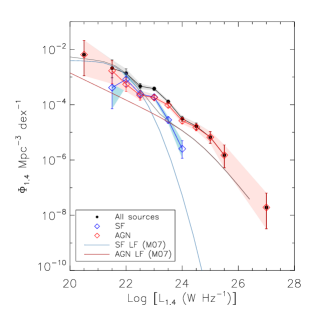
Figure 12: The blue diamonds are the RLF for SF sources, the red diamonds are for the AGN RLF and black is the total. The solid pale blue and pink lines are the parametric fits to the local RLF from Mauch & Sadler (2007). Errors are Poisson.

To demonstrate the completeness of our radio data, Figure 13 plots the radio luminosity against redshift with flux limits overplotted. For example, in ATLAS, radio sources with powers of 10²³ W Hz^-1 may be detected to z $\sim$ 0.4. The dashed line in Figure 13 shows the flux density limit for the study from Mauch & Sadler (2007). The dotted line in Figure 13 shows the flux density limit for the COSMOS survey (Scoville et al. 2007). Smolčić et al. (2009) calculated the RLF for low-power AGN in the COSMOS sample using predominately photometric redshifts and found mild evolution to z$\sim$1.3.

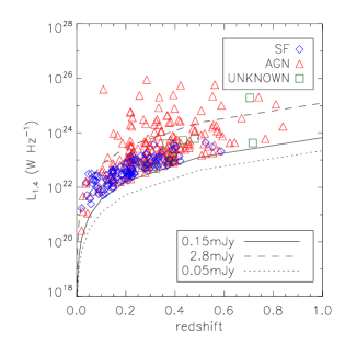
Figure 13: Radio luminosity plotted against redshift for our sources. The lines show different flux density limits. The solid line corresponds to a flux limit of 150 $\mu$Jy beam^-1, which is $\sim$5 $\times$ rms for our data. The dashed line corresponds to the flux density limit for Mauch & Sadler (2007) and the dotted line corresponds to the flux density limit for COSMOS (Smolčić et al. 2009).

4.5 RLF for SF galaxies

The RLF for SF galaxies has been proposed to evolve positively with redshift (e.g. Rowan-Robinson et al. 1993; Hopkins et al. 1998). We compare our RLF for SF galaxies with that of previous work by Afonso et al. (2005) and Mauch & Sadler (2007) (Figure 14 and Table 4). Although the total SF galaxy RLF for our dataset is higher than the SF galaxy RLF of Mauch & Sadler (2007) – especially for more luminous sources – this is attributed to cosmic evolution. When the SF galaxy RLF is separated into two redshift bins it is apparent that the low redshift bin is in good agreement with Mauch & Sadler (2007). Afonso et al. (2005) found their data were consistent with pure luminosity evolution in the form L${}_{1.4\,GHz}\propto$ (1+z)^Q, with $Q=2.7\pm 0.6$ (Hopkins 2004). Our dataset has very similar optical and radio limits to Afonso et al. (2005), and we find our SF RLF to agree within the uncertainties with theirs at both redshift bins.

Table 4: Radio luminosity function at 1.4 GHz for SF galaxies and AGN in ELAIS at two different redshift bins.

		SF 0$<$z$\leq$0.2		SF 0.2$<$z$\leq$0.5		AGN 0$<$z$\leq$0.2		AGN 0.2$<$z$\leq$0.4		AGN 0.4$<$z$\leq$0.8
log10L1.4	N	log${}_{10}\Phi$	N	log${}_{10}\Phi$	N	log${}_{10}\Phi$	N	log${}_{10}\Phi$	N	log${}_{10}\Phi$
(W Hz-1)		(Mpc-3 dex-1)		(Mpc-3 dex-1)		(Mpc-3 dex-1)		(Mpc-3 dex-1)		(Mpc-3 dex-1)
20.5	0		0		1	-2.19${}_{-0.76}^{+0.52}$	0		0
21.0	0		0		0		0		0
21.5	1	-3.38${}_{-0.76}^{+0.52}$	0		2	-2.77${}_{-0.47}^{+0.37}$	0		0
22.0	5	-3.08${}_{-0.26}^{+0.23}$	0		5	-3.26${}_{-0.26}^{+0.23}$	0		0
22.5	8	-3.78${}_{-0.19}^{+0.17}$	8	-3.25${}_{-0.19}^{+0.17}$	6	-3.73${}_{-0.23}^{+0.20}$	3	-3.62${}_{-0.34}^{+0.30}$	0
23.0	8	-3.89${}_{-0.19}^{+0.17}$	24	-3.63${}_{-0.10}^{+0.10}$	5	-3.90${}_{-0.26}^{+0.23}$	27	-3.64${}_{-0.09}^{+0.09}$	1	-5.03${}_{-0.76}^{+0.52}$
23.5	0		16	-4.49${}_{-0.12}^{+0.12}$	2	-4.35${}_{-0.49}^{+0.37}$	35	-3.97${}_{-0.08}^{+0.08}$	11	-4.43${}_{-0.15}^{+0.15}$
24.0	0		3	-5.46${}_{-0.34}^{+0.30}$	1	-4.49${}_{-0.83}^{+0.52}$	11	-4.53${}_{-0.15}^{+0.15}$	10	-4.95${}_{-0.16}^{+0.15}$
24.5	0		0		0		7	-4.71${}_{-0.20}^{+0.19}$	7	-4.98${}_{-0.20}^{+0.19}$
25.0	0		0		0		5	-4.87${}_{-0.25}^{+0.22}$	1	-6.10${}_{-0.77}^{+0.52}$
25.5	0		0		0		1	-5.69${}_{-0.77}^{+0.52}$	1	-5.83${}_{-0.77}^{+0.52}$
Total	22		51		22		89		31
$<$V/V${}_{\rm MAX}>$		0.632$\pm$ 0.039		0.480$\pm$ 0.019		0.526$\pm$ 0.032		0.548$\pm$ 0.017		0.578$\pm$ 0.030

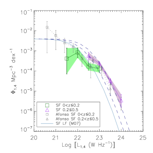
Figure 14: Radio luminosity function for SF galaxies in ATLAS. We have split our data into two redshift bins so as to allow for direct comparison against Afonso et al. (2005). The grey data points are from Afonso et al. (2005). Errors are Poisson. The parametric fit to the SF RLF from Mauch & Sadler (2007) is also shown, both in its original form and after applying luminosity evolution in the form L${}_{1.4\,GHz}\propto$ (1+z)^Q, with $Q=2.7\pm 0.6$ (Hopkins 2004) and z = 0.2 and z = 0.5.

4.6 RLF For AGN

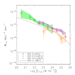
Figure 15: Radio luminosity function for AGN in ATLAS-ELAIS. We have split our data into three redshift bins. The pink line is the local AGN RLF from Mauch & Sadler (2007). Errors are Poisson.

To determine the cosmic evolution of the RLF for AGN, we bin the data in redshift and compute the RLFs for each redshift bin. Figure 15 and Table 4 show the RLFs for the three redshift bins. We compare our AGN RLF with Mauch & Sadler (2007) and find that our data is systematically inconsistent with the AGN RLF from Mauch & Sadler (2007), being a factor of $\sim$3 higher.

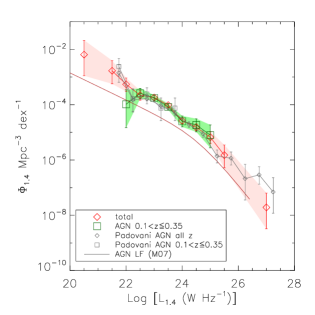
Figure 16: Radio luminosity function for AGN in ATLAS-ELAIS with data from Padovani et al. (2011) overplotted. Both the total AGN RLF and the RLF for the redshift range $0.1<$ z $\leq 0.35$ are plotted to allow direct comparison with Padovani et al. (2011). The pink line is the local AGN RLF from Mauch & Sadler (2007). Errors are Poisson.

Padovani et al. (2011) calculated the RLF for AGNs using the VLA-CDFS sample (Kellermann et al. 2008) and also find their RLF to be a factor of 3 – 4 higher than Mauch & Sadler (2007), predominately due to the population of “radio-quiet” AGNs that cannot be detected in less sensitive surveys. We compare our data with theirs over the same redshift range and find them to be in good agreement (Figure 16).

4.6.1 Why is our AGN RLF ‘high’?

The AGN RLF for ELAIS is puzzling as it appears inconsistent with the local AGN RLF of Mauch & Sadler (2007). For example, the median redshift for the eight lowest luminosity AGN (the left-most three green data points in Figure 15) is z $\sim 0.05$, which is comparable to the median redshift of z $\sim 0.07$ from Mauch & Sadler (2007). We specifically investigate whether these eight sources may have been mis-classified in some way. Four of the eight have clear evidence for AGN acitivity in their optical spectra (e.g. broad lines, high NII/H$\alpha$ ratios etc) and the other four have early-type spectra. The one source that also had sufficient mid-infrared data is likely to be AGN as it has mid-infrared colours consistent with other early-type galaxies.

The AAOmega spectra are obtained through fibres 2 arcsec in diameter, which corresponds to a projected diameter of 6.4 kpc at z=0.2. Consequently, in the cases where we detect an early-type spectrum, it is possible that we are only seeing the bulge of a star-forming galaxy (see e.g. Mauch & Sadler 2007). This is supported by the fact that the total RLF in Figure 12 agrees very well with Mauch & Sadler (2007) at L${}_{1.4\,GHz}<10^{22.5}$ W Hz^-1, but the SF RLF is lower and the AGN RLF is higher.

The next redshift slice, $0.2<\rm z\leq 0.4$ is equally puzzling as it too is a factor of $\sim$ 3 higher than the local AGN RLF. Some of this may be attributed to evolution, although the large error bars preclude us from drawing any strong conclusions. We note the further possibility that these sources are hybrid in nature, and it is possible for a source to have both a star-forming disk and a nuclear AGN. While an investigation into this would be useful, it is beyond the scope of this paper.

Another factor contributing to the higher number density of AGN may be the presence of clusters or other large-scale structures, which can have the effect of inflating the AGN RLF in ELAIS due to the small volumes probed (e.g. Padovani et al. 2011). For example, Mao et al. (2010a) detected a large overdensity at z $\sim 0.2$ associated with a wide-angle tailed galaxy. The removal of galaxies in this overdensity lowers the overall AGN RLF, although not by a significant amount ($\delta\Phi<15\%$). However, there are three additional WATs in ELAIS (Mao et al. 2010a) at $0.3<$ z $<0.4$, each of which is likely to be associated with a cluster. The sampling of a larger volume would mitigate the effects of cosmic variance.

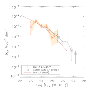
Figure 17: Radio luminosity function for AGN in ATLAS-ELAIS with data from Sadler et al. (2007) overplotted. The RLF for the redshift range $0.4<$ z $\leq 0.7$ is plotted to allow direct comparison with Sadler et al. (2007). The pink line is the local AGN RLF from Mauch & Sadler (2007). Errors are Poisson.

Sadler et al. (2007) calculated the RLF for AGNs at $0.4<$ z $\leq 0.7$ using radio data from FIRST and optical data from 2SLAQ. We compare our data with theirs over the same redshift range and find them to be in good agreement (Figure 17). At this redshift range we should be probing a volume large enough to sample the Universe fairly and hence be free of the effects of cosmic variance.

We are not able to determine definitively why the AGN RLF for ELAIS appears to be ‘high’. We have explored the possibility of evolution, cosmic variance and the possibility of spectra being unrepresentative of the source. The AGN RLF may be suffering the effects of any one of these factors, or possibly a combination. DR3 will provide this study with more data so that we may determine why our AGN RLF is high.

5 Summary and Conclusions

We have presented 466 new spectroscopic redshifts for radio sources in ELAIS and CDFS as part of ATLAS, using AAOmega on the AAT. We have classified the sources as AGN or SF based on their spectra and compared these spectroscopic classifications with mid-IR diagnostics and found them to be in good agreement. Of the 466 sources, 282 are AGN, 142 are SF, 32 are either SF or AGN (none of the diagnostics used in this paper were able to determine if they were SF or AGN) and 10 are chance alignments with stars.

We have constructed the RLF for ELAIS for both SF galaxies and AGN. We find positive evolution, consistent with previous studies, to z = 0.5 for the SF RLF. We find our AGN RLF to be consistent with previous work by Padovani et al. (2011), and a factor of $\sim$3 higher than the work by Mauch & Sadler (2007).

We cannot make any definitive statements as to why the SF RLF for ELAIS is consistent with previous studies whereas the AGN RLF for ELAIS appears inconsistent. We attribute the inconsistencies to the possibility of evolution, cosmic variance, obtaining spectra of only the bulge of a SF galaxy leading to an overestimate of early-type galaxies, or possibly an amalgamation of all these factors. We shall perform these analyses on DR3 where the extra data will allow us to draw more definitive conclusions.

ATLAS is the pathfinder for the forthcoming EMU Survey (Norris et al. 2011a), planned for the new ASKAP telescope (Johnston et al. 2008), which will survey the entire visible sky to an rms depth of 10$\,\mu$Jy beam^-1. Because the ATLAS and EMU surveys are well-matched in sensitivity and resolution, the results obtained in this and other papers on the ATLAS survey will be used to guide the survey design and early science papers for EMU. In particular, the spectroscopy on ATLAS sources will provide a valuable training set to guide the algorithms used to determine the redshift distribution of the anticipated 70 million EMU sources.

Appendix A Redshifts for 24 $\mu$m excess sources

Redshifts for 697 of 1080 non-ATLAS sources were obtained. 472 of these are 24$\,\mu$m excess sources and form the basis of further investigation into the radio-FIR correlation (Norris et al., in preparation). Their redshifts were determined in the process of determining ATLAS redshifts and are presented here for the first time in Figure 5.

Table 5: First 10 lines of the catalogue of new spectrosopic redshifts for 24 $\mu$m excess sources in ATLAS.

SID	RA	Dec	z
	(J2000)	(J2000)
SWIRE3 J033350.32-280807.2	3:33:50.32	-28:08:07.30	0.2885
SWIRE3 J033300.84-280957.3	3:33:00.84	-28:09:57.30	0.2147
SWIRE3 J033246.75-280846.9	3:32:46.76	-28:08:47.00	3.1880
SWIRE3 J033223.92-281126.8	3:32:23.92	-28:11:26.80	0.1961
SWIRE3 J033221.93-281005.8	3:32:21.94	-28:10:05.90	0.1811
SWIRE3 J033347.81-281622.0	3:33:47.82	-28:16:22.00	0.1029
SWIRE3 J033159.87-280953.0	3:31:59.87	-28:09:53.00	0.2363
SWIRE3 J033154.67-281035.9	3:31:54.67	-28:10:36.00	0.2148
SWIRE3 J033417.62-281712.8	3:34:17.62	-28:17:12.90	0.3400
SWIRE3 J033237.30-280847.2	3:32:37.30	-28:08:47.30	0.7683

Appendix B V_enclosed/V_available

The ELAIS radio image is $\sim$4.7 square degrees, of which $\pi$ square degrees were observed with the AAT. In Figure 9 we presented the rms at each radio source position. Figure 18 presents the same data with the AAOmega field-of-view overlaid.

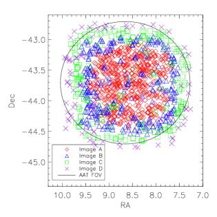
Figure 18: RA-Dec plot of ELAIS’s rms characteristics, with four different rms bins chosen, and colour-coded. To keep the plot simple, only parts of the image that aren’t also part of a deeper image are plotted. That is, Image D covers the entire radio image, and Image C’s datapoints can be thought of as being overlaid on Image D. The field-of-view of AAOmega is overlaid.

We can treat this non-uniform radio image as four overlapping radio images each with a different rms. Table 6 presents these areas, designated images A - D with A being the deepest and D being the shallowest image. The following equations and analyses are based on the equations provided in Avni & Bahcall (1980).

Table 6: The rms limits for the four overlapping radio images ELAIS is broken down into.

Image	RMS limit	Area
	($\mu$Jy beam-1)	(deg2)
A	30	0.95
B	40	1.75
C	65	2.56
D	100	3.14

Although whether the source is detected is both a function of the source’s position in the field, and its luminosity, the actual volume available to the source is dependent only upon its luminosity. That is to say, the source may be distributed anywhere within the total volume. This is because the volume available to the source is bound by the flux density limits presented in Table 6.

For a source of a given luminosity, the volume available (in Mpc³) to a source in our sample is

$$\rm V_{available} = \frac{1}{4\pi}\frac{4}{3}\pi(\Omega_{\rm(D-C)}\rm D_{MMAX,D}^{3}$$ (7)

$$+\Omega_{(C-B)}\rm D_{MMAX,C}^{3}$$

$$+\Omega_{\rm(B-A)}\rm D_{MMAX,B}^{3}$$

$$+\Omega_{A}\rm D_{MMAX,A}^{3})$$

$$= \frac{1}{3}(\Omega_{\rm(D-C)}\rm D_{MMAX,D}^{3}$$

$$+\Omega_{\rm(C-B)}\rm D_{MMAX,C}^{3}$$

$$+\Omega_{\rm(B-A)}\rm D_{MMAX,B}^{3}$$

$$+\Omega_{A}\rm D_{MMAX,A}^{3})$$

where $\Omega_{X}$ is the solid angle (in steradians) subtended by the image X, and D_MMAX,X is the maximum comoving distance in Mpc for image X. In this way, each source is accounted for only once. This corresponds to Equation 9 of Avni & Bahcall (1980).

The actual volume enclosed by the source, corresponding to Equation 10 of Avni & Bahcall (1980), is dependent on the source’s redshift (and hence D_M,source). For a source whose redshift is less than the maximum redshift the shallowest image (D) can detect, the enclosed volume is simply

$$\rm V_{enclosed} = \frac{1}{3}(\Omega_{D}\rm D_{M,source}^{3})$$ (8)

where D_M,source is the comoving distance in Mpc for the source.

However, for a source whose redshift is less than or equal to the maximum redshift the deepest image (A) can detect, the enclosed volume is

$$\rm V_{enclosed} = \frac{1}{3}(\Omega_{(D-C)}\rm D_{MMAX,D}^{3}$$ (9)

$$+\Omega_{(C-B)}\rm D_{MMAX,C}^{3}$$

$$+\Omega_{(B-A)}\rm D_{MMAX,B}^{3}$$

$$+\Omega_{A}\rm D_{M,source}^{3})$$

This is shown schematically in Figure 19. These are for the two extremes but the same procedure is followed for sources with redshifts between z_MAX,C and z_MAX,D as well as for sources with redshifts between z_MAX,B and z_MAX,C.

Figure 19: A simple model depicting V_available (solid black line) and V_enclosed (shaded region) for a source whose redshift is less than the maximum redshift detectable in the shallowest image (upper panel) and for a source whose redshift is less than the maximum redshift detectable in the deepest image (lower panel). The x-axis is an idealised cross-section of the area and the y-axis is the redshift.

References

- Afonso et al. (2005) Afonso J., Georgakakis A., Almeida C., Hopkins A. M., Cram L. E., Mobasher B., Sullivan M., 2005, ApJ, 624, 135
- Antonucci (1993) Antonucci R., 1993, ARA&A, 31, 473
- Avni & Bahcall (1980) Avni Y., Bahcall J. N., 1980, ApJ, 235, 69
- Becker, White, & Helfand (1995) Becker R. H., White R. L., Helfand D. J., 1995, ApJ, 450, 559
- Bennett (1962) Bennett A. S., 1962, MmRAS, 68, 163
- Best & Heckman (2012) Best P. N., Heckman T. M., 2012, arXiv, arXiv:1201.2397
- Chary & Elbaz (2001) Chary R., Elbaz D., 2001, ApJ, 556, 562
- Clewley & Jarvis (2004) Clewley L., Jarvis M. J., 2004, MNRAS, 352, 909
- Colless et al. (2001) Colless M., et al., 2001, MNRAS, 328, 1039
- Condon (1992) Condon J. J., 1992, ARA&A, 30, 575
- Condon et al. (1998) Condon J. J., Cotton W. D., Greisen E. W., Yin Q. F., Perley R. A., Taylor G. B., Broderick J. J., 1998, AJ, 115, 1693
- Croom et al. (2004) Croom S. M., Smith, R. J., Boyle, B. J., et al., 2004, MNRAS, 349, 1397
- Croton et al. (2006) Croton D. J., et al., 2006, MNRAS, 365, 11
- De Propris et al. (2004) De Propris R., et al., 2004, MNRAS, 351, 125
- Dunlop & Peacock (1990) Dunlop J. S., Peacock J. A., 1990, MNRAS, 247, 19
- Edge et al. (1959) Edge D. O., Shakeshaft J. R., McAdam W. B., Baldwin J. E., Archer S., 1959, MmRAS, 68, 37
- Gehrels (1986) Gehrels N., 1986, ApJ, 303, 336
- Giavalisco et al. (2004) Giavalisco M., et al., 2004, ApJ, 600, L93
- Gieseke et al. (2011) Gieseke F., Polsterer K. L., Thom A., Zinn P.-C., Bomanns D., Dettmar R.-J., Kramer O., Vahrenhold J., 2011, arXiv, arXiv:1108.4696
- Glazebrook & Bland-Hawthorn (2001) Glazebrook K., Bland-Hawthorn J., 2001, PASP, 113, 197
- Hardcastle, Evans, & Croston (2007) Hardcastle M. J., Evans D. A., Croston J. H., 2007, MNRAS, 376, 1849
- Hambly et al. (2001) Hambly N. C., et al., 2001, MNRAS, 326, 1279
- Hogg (1999) Hogg D. W., 1999, astro, arXiv:astro-ph/9905116
- Hopkins et al. (1998) Hopkins A. M., Mobasher B., Cram L., Rowan-Robinson M., 1998, MNRAS, 296, 839
- Hopkins (2004) Hopkins A. M., 2004, ApJ, 615, 209
- Huynh, Jackson, & Norris (2007) Huynh M. T., Jackson C. A., Norris R. P., 2007, AJ, 133, 1331
- Ibar et al. (2010) Ibar E., Ivison R. J., Best P. N., Coppin K., Pope A., Smail I., Dunlop J. S., 2010, MNRAS, 401, L53
- Johnston et al. (2008) Johnston S., et al., 2008, ExA, 22, 151
- Kellermann et al. (2008) Kellermann K. I., Fomalont E. B., Mainieri V., Padovani P., Rosati P., Shaver P., Tozzi P., Miller N., 2008, ApJS, 179, 71
- Kimball et al. (2011) Kimball A. E., Kellermann K. I., Condon J. J., Ivezić Ž., Perley R. A., 2011, ApJ, 739, L29
- Lacy et al. (2004) Lacy M., et al., 2004, ApJS, 154, 166
- Lacy et al. (2007) Lacy M., Petric A. O., Sajina A., Canalizo G., Storrie-Lombardi L. J., Armus L., Fadda D., Marleau F. R., 2007, AJ, 133, 186
- Lonsdale et al. (2003) Lonsdale C. J., et al., 2003, PASP, 115, 897
- Mao et al. (2010a) Mao M. Y., Sharp R., Saikia D. J., Norris R. P., Johnston-Hollitt M., Middelberg E., Lovell J. E. J., 2010a, MNRAS, 406, 2578
- Mao et al. (2010b) Mao M. Y., Norris R. P., Sharp R., Lovell J. E. J., 2010b, IAUS, 267, 119
- Mauch et al. (2003) Mauch T., Murphy T., Buttery H. J., Curran J., Hunstead R. W., Piestrzynski B., Robertson J. G., Sadler E. M., 2003, MNRAS, 342, 1117
- Mauch & Sadler (2007) Mauch T., Sadler E. M., 2007, MNRAS, 375, 931
- McAlpine & Jarvis (2011) McAlpine K., Jarvis M. J., 2011, MNRAS, 413, 1054
- Middelberg et al. (2008) Middelberg E., et al., 2008, AJ, 135, 1276
- Miller et al. (2008) Miller N. A., Fomalont E. B., Kellermann K. I., Mainieri V., Norman C., Padovani P., Rosati P., Tozzi P., 2008, ApJS, 179, 114
- Moster et al. (2011) Moster B. P., Somerville R. S., Newman J. A., Rix H.-W., 2011, ApJ, 731, 113
- Norris et al. (2006) Norris R. P., et al., 2006, AJ, 132, 2409
- Norris et al. (2011a) Norris R. P., et al., 2011a, PASA, 28, 215
- Norris et al. (2011b) Norris R. P., Lenc E., Roy A. L., Spoon H., 2011b, arXiv, arXiv:1107.3895
- Owen & Morrison (2008) Owen F. N., Morrison G. E., 2008, AJ, 136, 1889
- Padovani et al. (2009) Padovani P., Mainieri V., Tozzi P., Kellermann K. I., Fomalont E. B., Miller N., Rosati P., Shaver P., 2009, ApJ, 694, 235
- Padovani et al. (2011) Padovani P., Miller N., Kellermann K. I., Mainieri V., Rosati P., Tozzi P., 2011, ApJ, 740, 20
- Pope, Mendel, & Shabala (2012) Pope E. C. D., Mendel J. T., Shabala S. S., 2012, MNRAS, 419, 50
- Randall et al. (2012) Randall K. E., Hopkins A. M., Norris R. P., Zinn P.-C., Middelberg E., Mao M. Y., Sharp R. G., 2012, MNRAS, 2478
- Richards et al. (2006) Richards G. T., et al., 2006, ApJS, 166, 470
- Rowan-Robinson et al. (1993) Rowan-Robinson M., Benn C. R., Lawrence A., McMahon R. G., Broadhurst T. J., 1993, MNRAS, 263, 123
- Rowan-Robinson et al. (2008) Rowan-Robinson M., et al., 2008, MNRAS, 386, 697
- Sadler et al. (1999) Sadler E. M., McIntyre V. J., Jackson C. A., Cannon R. D., 1999, PASA, 16, 247
- Sadler et al. (2002) Sadler E. M., et al., 2002, MNRAS, 329, 227
- Sadler et al. (2007) Sadler E. M., et al., 2007, MNRAS, 381, 211
- Sajina, Lacy, & Scott (2005) Sajina A., Lacy M., Scott D., 2005, ApJ, 621, 256
- Saunders et al. (2004) Saunders W., et al., 2004, SPIE, 5492, 389
- Schinnerer et al. (2007) Schinnerer E., et al., 2007, ApJS, 172, 46
- Schmidt (1968) Schmidt M., 1968, ApJ, 151, 393
- Schmidt (1977) Schmidt M., 1977, IAUS, 74, 259
- Scoville et al. (2007) Scoville N., et al., 2007, ApJS, 172, 1
- Seymour et al. (2008) Seymour N., et al., 2008, MNRAS, 485
- Shabala et al. (2011) Shabala S. S., et al., 2011, arXiv, arXiv:1107.5310
- Sharp et al. (2006) Sharp R., et al., 2006, SPIE, 6269,
- Sharp & Parkinson (2010) Sharp R., Parkinson H., 2010, MNRAS, 408, 2495
- Smolčić et al. (2008) Smolčić V., et al., 2008, ApJS, 177, 14
- Smolčić et al. (2009) Smolčić V., et al., 2009, ApJ, 696, 24
- Stern et al. (2005) Stern D., et al., 2005, ApJ, 631, 163
- Tonry & Davis (1979) Tonry J., Davis M., 1979, AJ, 84, 1511
- Wilson et al. (2011) Wilson W. E., et al., 2011, MNRAS, 416, 832
- Wright (2006) Wright E. L., 2006, PASP, 118, 1711