Separation of spacetime and matter in polar oscillations of compact stars

Abstract

The dynamics of polar oscillations of compact stars are conventionally described by a set of coupled differential equations, and the roles that spacetime and matter play in such oscillations are consequently difficult to track. In the present paper, we develop a scheme for polar oscillations in terms of one spacetime and one matter variables. With our judicious choice of variables, the coupling between spacetime and matter is weak, which enables the separation of these two parties. Two independent second-order ordinary differential equations are obtained, corresponding to the Cowling and inverse-Cowling approximations, and leading to accurate determination of p and w-mode quasi-normal modes, respectively, in a unified framework.

1 Introduction

Compact stars, including neutron stars (NSs) and quark stars (QSs), are notable for the high density achievable at their centers and the huge gravitational field surrounding them. Their internal structure is often the ideal test bed for the equation of state (EOS) of nuclear (or quark) matter and can provide clues to the interactions between elementary particles as well (see, e.g., Glendenning 1997, Lattimer & Prakash 2007, Weber 1999, Lattimer 2012, and references therein). Gravitational waves (GWs) emitted from oscillating NSs (or QSs) are expected to carry rich information about their internal structures and hence the physics of dense matter as well, giving rise to various efforts to infer the properties of relativistic compact stars from close examination of their oscillation spectra (see, e.g., Andersson & Kokkotas 1996, 1998, Benhar et al. 1999, Kokkotas et al. 2001, Benhar et al. 2004, Tsui & Leung 2005a, Tsui et al. 2006, Lau et al. 2010, Sotani et al. 2011, Doneva et al. 2013). Although the oscillation frequencies of NSs usually lie outside the sensitivity window of the existing GW detectors such as GEO600, LIGO I, TAMA300 and VIRGO (see, e.g., Hughes 2003, Fryer et al. 2002), with the advent of more sensitive third-generation GW telescopes (e.g., the proposed Einstein Telescope, see Andersson et al. 2011, Hild et al. 2011), it is probable that the structure and the composition of a compact star can be inferred from its GW signals in the coming future.

The fully relativistic formulation of stellar pulsations was first founded by Thorne & Campolattaro (1967) and since then alternative approaches to such processes have emerged in the literature (see, e.g., Lindblom & Detweiler 1983, Detweiler & Lindblom 1985, Chandrasekhar & Ferrari 1991, Lindblom et al. 1997, Kokkotas & Schmidt 1999a). Basically, oscillations of compact stars are classified into axial and polar types. For axial type oscillations, the matter forming a star is essentially a spectator and only the spacetime surrounding the star pulsates. For polar type oscillations, matter motion and spacetime variation are, however, coupled together. To describe such coupled motion, different forms of equations of motion have been proposed since the pioneering work of Thorne & Campolattaro (1967). For example, based on Thorne & Campolattaro (1967), Lindblom & Detweiler (1983) and Detweiler & Lindblom (1985) described the system with four coupled first-order ODEs in four variables (termed as the LD formalism in this paper), which can be readily solved numerically. Later, to draw an analogy between the oscillations of relativistic and Newtonian stars, Lindblom et al. (1997) proposed a new formalism to describe the coupled oscillation with two second-order equations (termed as the LMI formalism), which reduce directly into the corresponding Newtonian equations under the weak field limit. In another relativistic stellar pulsation formalism proposed by Allen et al. (1998) (termed as the AAKS formalism in this paper), variations in matter and spacetime are described by one matter variable and two metric variables. The three variables are governed by three coupled second-order time-dependent wave equations. Allen et al. (1998) managed to evolve these three variables numerically in the time domain for certain sets of initial conditions and studied the characteristics of the GWs emitted in such cases.

Polar type oscillations are very much involved in dynamical processes such as supernova and binary mergers of NSs. The interplay between spacetime and matter in polar oscillations of compact stars, however, often poses hurdles for developing a firm grasp of these phenomena. To trace the individual roles played by matter and spacetime components, different variants of the Cowling approximation (CA), where effects of metric perturbations are neglected (McDermott et al. 1983, Finn 1988, Lindblom & Splinter 1990, Lindblom et al. 1997), and the inverse-Cowling approximation (ICA), where fluid motion is ignored (Andersson et al. 1996, Wu & Leung 2007), have been proposed. These approximations vary in the choice of the physical variable measuring the matter or spacetime component and lead to different degrees of accuracy (see the above-mentioned references).

In the present paper, we study polar oscillations with quasi-normal mode (QNM) analysis. QNMs are oscillation modes with all dynamical variables decay exponentially in time (Press 1971, Leaver 1986, Ching et al. 1998, Kokkotas & Schmidt 1999a, Berti et al. 2009, Konoplya & Zhidenko 2011). Mathematically, the perturbation variables are assumed to have the $e^{-i\omega t}$ dependence , where the eigenfrequency $\omega\equiv\omega_{\rm r}-i\omega_{\rm i}$ is complex-valued with $\omega_{\rm i}\geq 0$ measuring the decay rate of the mode. QNMs of compact stars reveal the physical characteristics (e.g., mass, radius, moment of inertia, EOS and composition) of a star (see, e.g., Andersson & Kokkotas 1996, 1998, Benhar et al. 1999, Kokkotas et al. 2001, Benhar et al. 2004, Tsui & Leung 2005a, Tsui et al. 2006, Lau et al. 2010). Polar QNMs of compact stars can be classified into the fluid mode, including the fundamental $f$-mode, the pressure $p$-mode and the gravity $g$-mode according to the nature of respective restoring forces (Cowling 1941), and the spacetime $w$-mode which has no Newtonian counterpart.

The aim of the present paper is to propose a physically more transparent picture for polar oscillations of compact stars. Two coupled second-order differential equations in the frequency domain, involving one matter field and one spacetime variable used in the AAKS formalism, are derived (see Section 2 and Appendix A). Our judicious choice of the two variables enables a straightforward decoupling of the two equations, leading to two independent equations accurately describing fluid modes (especially $p$-modes) and the $w$-modes, respectively (see Section 3). Hence, in a unified framework, we simultaneously establish both CA and ICA, which can lead to much improved accuracies in comparison with other approximation schemes proposed previously (see Sections 4 and 5 respectively). Under the current CA, fluid motion is governed by a Sturm-Liouville eigenvalue system, where completeness and orthogonality relations hold as usual (see, e.g., Morse & Feshbach 1953). Therefore, the fluid system is a conservative one and can be studied with conventional normal-mode analysis. The mode with the lowest eigenfrequency indeed corresponds to the $f$-mode, while the following modes are good approximations for the successive $p$-modes. Besides, we also find that other variants of CA (McDermott et al. 1983, Finn 1988) can also be recast into a form analogous to ours, save the difference in two parameters. As regards the present ICA, to our knowledge, this is the first time that an approximate single second-order differential equation describing polar $w$-mode QNMs, which has been numerically verified to lead accuracies much better than one percent, has been formulated.

Geometric units in which $G=c=1$ are adopted throughout this paper. We consider polar oscillations of a non-rotating compact star of perfect fluid with radius $R$ and total mass $M$. Unless stated otherwise, all numerical values of frequencies are measured in units of $M^{-1}$ and evaluated for the case where the angular momentum index $l$ equals 2. Besides, we also assume that the effect of temperature on the EOS of nuclear matter is negligible and hence $g$-modes are omitted in our discussion. In order not to divert the reader’s attention from the main physical findings achieved in the paper, we put most of the mathematical details in three appendices.

2 Two-variable scheme for Polar QNMs

2.1 Three-variable scheme

When a static compact star is perturbed, its fluid and spacetime acquire small-amplitude, time-dependent perturbations about the equilibrium state. These perturbations are first decomposed into tensorial and vectorial spherical harmonics $Y_{lm}(\theta,\psi)$ with angular momenta $\{lm\}$, and then separated into axial and polar parts according to parity. The perturbed line element of polar parity in the Regge-Wheeler gauge is (Thorne & Campolattaro 1967, Regge & Wheeler 1957, Price & Thorne 1969, Kojima 1992):

$$ds^{2}\!\!\!\!\! = \!\!\!\!\!-e^{\nu}(1-H_{0}Y_{lm})dt^{2}+e^{\lambda}(1+H_{0}Y_{lm})dr^{2}$$ (1)

$$\!\!\!\!\!+2H_{1}Y_{lm}dtdr+r^{2}(1+KY_{lm})(d\theta^{2}+\sin^{2}\theta d\phi^{2}),$$

where the convention of the metric follows that used in Kojima (1992), and $e^{\nu}$ and $e^{\lambda}$ are characteristics of the star at equilibrium (see, e.g., Chapter 2, Glendenning 1997).

In the AAKS formalism (Allen et al. 1998), polar oscillations of compact stars are described by two spacetime metric variables $F$, $S$ and one fluid perturbation variable $H$, which are related to the above metric perturbations and the Eulerian change in pressure $\delta{p}$ as follows:

$$S\!\!\!\!\! = \!\!\!\!\!e^{\nu}(H_{0}-K)/r,$$

$$F\!\!\!\!\! = \!\!\!\!\!rK,$$

$$H\!\!\!\!\! = \!\!\!\!\!\delta p/(\rho+p).$$ (2)

The three variables $S$, $F$ and $H$ satisfy three coupled second-order differential equations and a Hamiltonian constraint (see Appendix A).

It has been shown that inside the star and in the weak field limit $K$ and $H_{0}$ are related to the perturbation in the Newtonian potential $U_{1}$ by (Thorne 1969):

$$K\simeq H_{0}\simeq 2U_{1}.$$ (3)

Therefore, following directly from (2), to leading orders in field strengths, $S$ and $F$ measure the relativistic and Newtonian effects of gravity, respectively. Hence, in order to describe generation of GWs, which is the dominant process in the spacetime mode, $S$ is the right variable to keep. On the other hand, $H$ is proportional to the Eulerian change in pressure and describes the motion of matter. We therefore eliminate the variable $F$ in the AAKS formalism and establish a scheme with one spacetime variable $S$ and one matter variable $H$.

2.2 Two-variable scheme

For QNMs, the three field variables in AAKS formalism take the time-dependence $e^{-i\omega t}$, e.g., $S(r,t)=S(r)e^{-i\omega t}$ and etc. A two-variable scheme is achievable by eliminating one of these three variables in the frequency domain. In particular, in the so-called $H$-$S$ scheme, the variable $F(r)$ and its derivative are expressed in terms of $S(r)$, $H(r)$ and their derivatives (see Appendix B). Two coupled second-order ODEs inside the star are then readily obtained:

$$\frac{d^{2}S}{dr_{*}^{2}}\!\!\!\!\! + \!\!\!\!\!U_{S1}(\omega,r)\frac{dS}{dr_{*}}+[\omega^{2}-V_{S0}(r)-U_{S0}(\omega,r)]S$$ (4)

$$= \!\!\!\!\!\Delta_{H1}(\omega,r)\frac{dH}{dr_{*}}+\Delta_{H0}(\omega,r)H,$$

$$\frac{d^{2}H}{dr_{*}^{2}}\!\!\!\!\! + \!\!\!\!\![V_{H1}(r)+U_{H1}(\omega,r)]\frac{dH}{dr_{*}}+[\frac{\omega^{2}}{C_{s}^{2}}-V_{H0}(r)$$ (5)

$$- \!\!\!\!\!U_{H0}(\omega,r)]H=\Delta_{S1}(\omega,r)\frac{dS}{dr_{*}}+\Delta_{S0}(\omega,r)S.$$

where

$$V_{S0}(r)\!\!\!\!\! = \!\!\!\!\!\frac{2e^{\nu}}{r^{3}}\left[(n+1)r-2\pi r^{3}(\rho+3p)-m\right],$$

$$V_{H0}(r)\!\!\!\!\! = \!\!\!\!\!\frac{2e^{\nu}}{r^{2}}\left[n+1-2\pi r^{2}(\rho+p)(3+\frac{1}{C_{s}^{2}})\right],$$

$$V_{H1}(r)\!\!\!\!\! = \!\!\!\!\!\frac{e^{(\nu+\lambda)/2}}{r^{2}}\left[(m+4\pi pr^{3})(1-\frac{1}{C_{s}^{2}})+2(r-2m)\right],$$

with $n=(l+2)(l-1)/2$, the tortoise coordinate $r_{*}(r)=\int_{0}^{r}e^{[\lambda(r^{\prime})-\nu(r^{\prime})]/2}dr^{\prime}$, and $C_{s}(r)\equiv(dp/d\rho)^{1/2}$ being the sound speed in the stellar fluid. The expressions of $U_{i}$ and $\Delta_{i}$, where $i=S0,S1,H0,H1$, can be found in Appendix B. Their contributions are typically much smaller than those of the $V$ terms. While $\Delta_{i}$ measure the interaction between $H$ and $S$, $U_{i}$ represent the effects of $F$ on the other two fields.

Outside the star, $H$ is identically zero and the system is described by only one second-order ODE in $S$:

$$\frac{d^{2}S}{dr_{*}^{2}}+U_{S1}(\omega,r)\frac{dS}{dr_{*}}+[\omega^{2}-V_{S0}(r)-U_{S0}(\omega,r)]S=0,$$ (6)

where all potential terms appearing in (6) can be obtained from their corresponding terms inside the star in (4) by setting $m(r)=M$, $\rho=p=0$.

2.3 Evaluation of QNMs

QNMs of vibrating compact stars are defined by the physical solutions of the proposed $S$ and $H$ equations with the spacetime variable $S$ satisfying the outgoing boundary condition $S\rightarrow\exp(i\omega r_{*}$) at spatial infinity. In solving the $S$-$H$ equation set inside the star, we numerically integrate (4) and (5) outward to find $S$ and $H$. First of all, the regularity boundary condition for $S$ and $H$ at $r=0$ leads to the asymptotic behavior $S\approx s_{0}r_{*}^{l+1}$ and $H\approx h_{0}r_{*}^{l}$ near the origin, where $s_{0}$ and $h_{0}$ are constants. By keeping only terms of order $1/C_{s}^{2}$ in (23) as $C_{s}\rightarrow 0$ when approaching the stellar surface, one can show that (Allen et al. 1998, Ruoff 2001):

$$-\omega^{2}{H}+\frac{M}{R^{2}}\frac{dH}{dr_{*}}-\frac{M}{2R^{3}}\frac{dF}{dr_{*}}+\frac{M}{2(R-2M)}\frac{dS}{dr_{*}}$$

$$+\frac{M(R+2M)F}{2R^{5}}+\frac{MS}{2R(R-2M)}=0.$$ (7)

Expressing $F$ and its derivative in terms of the other two variables, we can then impose the above boundary condition at the stellar surface to fix the ratio of $s_{0}$ to $h_{0}$ to obtain a unique (up to some multiplicative constant) solution of $S$ and $H$ inside the star. The inside and outside $S$ function is then connected at the star surface to determine the QNM frequencies.

In the following discussion, we will show that the $H$-$S$ approach achieved here naturally forms the basis of a decoupling scheme, and readily leads to accurate CA and ICA for $p$-modes and $w$-modes, respectively.

3 Separation of Spacetime and Matter

Dynamical processes such as supernova and binary mergers of NSs involve both spacetime variation and matter motion. Likewise, when a NS is perturbed away from equilibrium, the excitation energy is initially stored partially in the spacetime and partially in the matter. The energy stored in spacetime is damped out rapidly through the emission of $w$-mode gravitational waves owing to the short relaxation time (large imaginary part of eigenfrequency) of $w$-modes. On the other hand, the energy in matter has to be transferred into the spacetime through the coupling between matter and spacetime, which is measured by the $\Delta_{i}$ terms in (4) and (5), and is then brought away by fluid mode gravitational waves. The damping of fluid modes are usually slow due to the smallness of $\Delta_{i}$, leading to small imaginary parts of their eigenfrequencies, especially for $p$-modes.

Our choice of spacetime and matter variables provide a direct view on the weak coupling between spacetime and fluid mode oscillations. We therefore conclude that in fluid modes (especially the $p$-modes), the associated spacetime oscillations and hence GW emissions are almost negligible, whereas in the spacetime $w$-modes, fluid oscillations are hardly involved. This strongly suggests that the spacetime and matter in the developed schemes can be decoupled by taking the approximation $\Delta_{i}=0$ in (4) and (5):

$$\frac{d^{2}S}{dr_{*}^{2}}\!\!\!\!\! + \!\!\!\!\!U_{S1}(\omega,r)\frac{dS}{dr_{*}}+[\omega^{2}-V_{S0}(r)-U_{S0}(\omega,r)]S=0,$$ (8)

$$\frac{d^{2}H}{dr_{*}^{2}}\!\!\!\!\! + \!\!\!\!\![V_{H1}(r)+U_{H1}(\omega,r)]\frac{dH}{dr_{*}}+[\frac{\omega^{2}}{C_{s}^{2}}-V_{H0}(r)$$ (9)

$$- \!\!\!\!\!U_{H0}(\omega,r)]H=0.$$

4 Cowling Approximation for Fluid Modes

It is well known that the eigenfrequencies of the fluid modes, including both $f$ and $p$-modes, of a compact star are characterized by very small imaginary parts. The smallness of the imaginary part implies the tininess of GWs emitted in these modes, due to their weak couplings to spacetime variables. The decoupled equation for the fluid variable $H$ is given by (9) in Section 3. In the following, we further simplify it and develop a CA which is highly accurate for $p$-modes, and also works reasonably well for $f$-mode.

4.1 Fluid equation

The potentials $U_{H0}$ and $U_{H1}$ in (9) have a common denominator $D(\omega,r)$ (see Appendix B),

$$D\!\!\!\!\! = \!\!\!\!\!\omega^{4}+\omega^{2}\frac{e^{\nu}}{r^{4}}\left[e^{\lambda}(m+4\pi r^{3}p)^{2}+4mr+4\pi r^{4}(3p+\rho)\right]$$ (10)

$$+ \!\!\!\!\!\frac{2e^{2\nu}}{r^{6}}\left\{8\pi r^{3}(m+2\pi r^{3}p)(p+\rho)-e^{\lambda}(m+4\pi r^{3}p)^{2}\right.$$

$$\times \!\!\!\!\!\left.\left[1+n-8\pi r^{2}(p+\rho)\right]\right\},$$

which can drop to zero at a certain $r$ at low frequencies, typical of $f$-mode. On the other hand, $D(\omega,r)$ increases as $\omega^{4}$ at high frequencies, typical of $p$-modes. We find that for $p$-mode oscillations the effects of $U_{H0}$ and $U_{H1}$ are pretty small (both terms decreases as $1/\omega^{2}$), and further simplify (9) into:

$$\frac{d^{2}H}{dr_{*}^{2}}+V_{H1}(r)\frac{dH}{dr_{*}}+\left[\frac{\omega^{2}}{C_{s}^{2}}-V_{H0}(r)\right]H=0.$$ (11)

The above equation can also be derived by simply neglecting the $S$, $dS/dr_{*}$, $F$ and $dF/dr_{*}$ terms in $H$ equation in AAKS formalism (see Allen et al. 1998, and also Appendix A). Unlike $U_{H0}$ and $U_{H1}$, which are frequency-dependent, $V_{H0}$ and $V_{H1}$ are both frequency-independent. The mathematical structure of (11) is more desirable than (9) and leads to a complete orthonormal set of eigenfunctions. Eq. (9), on the other hand, properly accounts for the effects of $F$ on the fluid motion and is found to be the best available approximation for $p$-modes in the following discussion.

4.2 Boundary conditions

Under CA (11), $p$-mode oscillations are determined from (11) by imposing proper boundary conditions on $H$ at $r=0$ and $r=R$. Near the star center, $H\approx h_{0}r_{*}^{l}$ as mentioned previously. Assuming that the EOS acquires the polytropic form $p\propto\rho^{1+1/N}$ with the polytropic index $N>1$ near the star surface, which is typical for realistic NSs, we find that $C_{s}^{2}\sim A_{c}(R_{*}-r_{*})$ with $A_{c}=M/(R^{2}N)$ and $R_{*}$ being the tortoise radius of the star. Consequently, the $H$-equation near the stellar surface reduces asymptotically to

$$\frac{d^{2}H}{dr_{*}^{2}}-\frac{M}{R^{2}A_{c}(R_{*}-r_{*})}\frac{dH}{dr_{*}}+\frac{\omega^{2}}{A_{c}(R_{*}-r_{*})}H=0.$$

There are two independent solutions for this equation. The first one is bounded and behaves as:

$$H\propto\left[1+\omega^{2}R^{2}(r_{*}-R_{*})/M\right].$$ (12)

The other one is proportional to $(R_{*}-r_{*})^{1-N}$ and is unbounded. As $H$ is a physical quantity and must be finite at the stellar surface, it therefore follows (12).

The single $H$-equation (11) together with these two boundary conditions form an eigenvalue problem. The approximate eigenfrequencies of fluid modes under the CA can then be located.

4.3 Completeness and orthogonality

The eigenvalue problem of the purely matter-based $H$-equation (11) is actually a Sturm-Liouville eigenvalue problem, as it can be cast into the following standard form:

$$\frac{d}{dr_{*}}\left[P(r_{*})\frac{dH}{dr_{*}}\right]-Q(r_{*})H=-\omega^{2}\Lambda(r_{*})H,$$ (13)

with

$$P(r_{*})\!\!\!\!\! = \!\!\!\!\!e^{\nu}(\rho+p)r^{2},$$

$$Q(r_{*})\!\!\!\!\! = \!\!\!\!\!2e^{2\nu}(\rho+p)\left[n+1-2\pi r^{2}(\rho+p)(3+{1}/{C_{s}^{2}})\right],$$

$$\Lambda(r_{*})\!\!\!\!\! = \!\!\!\!\!e^{\nu}(\rho+p)r^{2}/{C_{s}^{2}}.$$

There are a series of real eigenfrequencies $\{\sigma_{n}\}$ and the corresponding normalized eigenfunctions $\{H_{n}(r_{*})\}$, which are defined by the boundary conditions derived above, namely (i) $H$ is regular at $r_{*}=0$, (ii) $(dH/dr_{*})/H=R^{2}\omega^{2}/M$ at $r=R_{*}$. Following straightforwardly from the standard theory of Sturm-Liouville system and the fact that $\Lambda(r=0)=0=\Lambda(r=R)$, the normalized eigenfunctions $\{H_{n}(r_{*})\}$ form a complete orthogonal set obeying the completeness and orthogonality relationships (see, e.g., Morse & Feshbach 1953):

$$\!\!\!\!\!\sum_{n}\Lambda(r_{*})H_{n}(r_{*})H_{m}(r_{*}^{\prime})=\delta(r_{*}-r_{*}^{\prime});$$ (14)

$$\!\!\!\!\!\int_{0}^{R_{*}}\Lambda(r_{*})H_{n}(r_{*})H_{m}(r_{*})dr_{*}=\delta_{nm}.$$ (15)

4.4 Numerical results and discussions

To gauge the accuracy of the CA developed (or ICA as discussed later) in the present paper, we use EOS A (Pandharipande 1971) to construct a NS with compactness ${\cal C}=0.27$ and central density $\rho_{c}=2.227\times 10^{-3}\textrm{km}^{-2}$ and evaluate the QNMs of the star. Table 1 shows the frequencies of the leading fluid modes obtained from exact calculation and CA (11) developed above. We see that the lowest eigenfrequency $\sigma_{0}$ of (13) provides us an approximate value of the real part of $f$-mode frequency, $\omega_{{\rm r},f}$, with a percentage error of around $20\%$. For $n\geq 1$, the eigenfrequency $\sigma_{n}$ yields an accurate approximation for the real part of the frequency of the $n$-th $p$-mode, $\omega_{{\rm r},p_{n}}$. The percentage error is usually much less than $1\%$ and decreases with increasing $n$ (see Table 1). The improvement in accuracy from $f$-mode to $p$-modes of the developed CA is expected. As the imaginary part of eigenfrequency decreases from $f$-mode to $p$-modes, the coupling between the spacetime and matter also gets weaker.

Table 1: Exact QNM frequency $(\omega_{\rm r},\omega_{\rm i})$ and the CA frequencies $\sigma_{n}$ obtained respectively from (11), (9), MVS (McDermott et al. 1983), Finn (Finn 1988), and LMI (Lindblom et al. 1997) CA’s, and (70) are compared for the leading fluid modes of an EOS A star (${\cal C}=0.27$).

Mode	Exact	(11)	(9)	MVS	Finn	LMI	(70)
	($\omega_{\rm r}$, $\omega_{\rm i}$)	$\sigma_{n}$	$\sigma_{n}$	$\sigma_{n}$	$\sigma_{n}$	$\sigma_{n}$	$\sigma_{n}$
$f$	(0.1447, 7.5E-5)	0.1163	NA	0.1664	0.1773	0.1665	NA
$p_{1}$	(0.3932, 3.0E-6)	0.3928	0.3934	0.4433	0.4806	0.3984	0.3903
$p_{2}$	(0.6130, 5.8E-7)	0.6135	0.6130	0.6489	0.7102	0.6159	0.6126
$p_{3}$	(0.7639, 5.3E-8)	0.7640	0.7639	0.7842	0.8525	0.7664	0.7636

We also compare the $H$-function obtained from (11) and the exact $H$-function for the same star (EOS A, ${\cal C}=0.27$). The comparison is shown in Fig. 1. The $H$-functions in developed CA and the exact AAKS formalism are normalized so that

$$\int_{0}^{R_{*}}\Lambda(r_{*})|H|^{2}dr_{*}=1\,.$$

Besides, we assume that the exact $H$-function is real at $r=R$. The numerical results again confirm that the CA proposed here is very accurate for $p$-modes. The discrepancy between the approximate and the exact wave functions grows larger for $f$-mode, which implies that the coupling between spacetime (i.e., $F$ and $S$) and matter is very weak for $p$-modes, but is not negligible for $f$-mode.

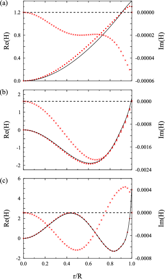
Figure 1: The normalized $H$-functions for (a) the $f$-mode; (b) the $p_{1}$-mode; and (c) the $p_{2}$-mode of a star constructed with EOS A ($\rho_{c}=2.227\times 10^{-3}\,\texttt{km}^{-2}$, ${\cal C}=0.27$) are plotted against the normalized radius $r/R$. The solid and the dashed lines are respectively the real and the imaginary parts of $H$-function under CA (11). The dots and crosses respectively show the real and the imaginary parts of the exact $H$-function.

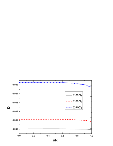
Figure 2: The function $D(\omega,r)$ is plotted against $r/R$ with $\omega=\sigma_{0},\sigma_{1},\sigma_{2}$.

Actually, as is mentioned before, the potentials $U_{i}$ and couplings $\Delta_{i}$ in the exact $H$ equation (5) have a common denominator $D(\omega,r)$ given by (10). It is clearly seen that the accuracy of the CA (11), would decrease if $D(\omega,r)$ is small. As is shown in Fig. 2, where $D$ is plotted against $r/R$ for different values of $\omega$ for the same star. $D$ decreases with decreasing $\omega$. In fact, for $\omega=\sigma_{0}$ (i.e., the $f$-mode frequency under CA), $D$ vanishes at $r/R=0.947$. Therefore, the omission of the influence of spacetime (i.e., $F$ and $S$) on oscillations of matter field may lead to appreciable errors at low frequencies. On the other hand, we observe that there are exactly $n$ nodes (excluding the origin) in the wave function $H_{n}$, in agreement with standard theory of the Sturm-Liouville eigen-system (see, e.g., Zettl 2005).

For the purpose of comparison, approximate eigenfrequencies obtained from (9) are also listed in Tables 1, 2 and 3. While Eq. (9) in general can yield almost exact numerical results for $p$-modes because it has properly taken the influence of $F$ on $H$ into consideration, it completely fails to locate approximate position of the $f$-mode. As mentioned above, the inability of (9) to handle the $f$-mode can be understood as a direct consequence of the fact that $D$ could vanish at certain positions inside the star at frequencies close to the $f$-mode frequency.

Table 2: Exact complex eigenfrequencies $(\omega_{\rm r},\omega_{\rm i})$ and approximate real eigenfrequencies $\sigma_{n}$ obtained respectively from CA (11), (9) and (70) are listed for the leading fluid modes of NSs constructed with the Sly EOS (Douchin & Haensel 2001, Haensel & Potekhin 2004) for different compactness ${\cal C}$. Entries labelled by ‘NA’ signify modes that cannot be located by a specific approximation.

${\cal C}$	Mode	Exact	(11)	(9)	(70)
		$(\omega_{\rm r},\omega_{\rm i})$	$\sigma_{n}$	$\sigma_{n}$	$\sigma_{n}$
0.117	$f$	(0.0488, 1.162E-5)	0.0410	NA	NA
0.117	$p_{1}$	(0.1654, 4.866E-7)	0.1651	0.1654	0.1628
0.117	$p_{2}$	(0.2079, 2.029E-8)	0.2079	0.2079	0.2071
0.117	$p_{3}$	(0.2390, 5.709E-9)	0.2390	0.2390	0.2383
0.210	$f$	(0.1047, 5.290E-5)	0.0848	NA	NA
0.210	$p_{1}$	(0.3281, 2.371E-6)	0.3279	0.3283	0.3245
0.210	$p_{2}$	(0.4995, 3.435E-8)	0.4996	0.4995	0.4985
0.210	$p_{3}$	(0.6154, 6.028E-9)	0.6155	0.6154	0.6150
0.276	$f$	(0.1476, 7.570E-5)	0.1177	NA	NA
0.276	$p_{1}$	(0.4074, 1.884E-6)	0.4072	0.4075	0.4053
0.276	$p_{2}$	(0.6236, 6.806E-7)	0.6241	0.6236	0.6234
0.276	$p_{3}$	(0.8192, 7.455E-8)	0.8195	0.8192	0.8193

Table 3: Exact complex eigenfrequencies $(\omega_{\rm r},\omega_{\rm i})$ and approximate real eigenfrequencies $\sigma_{n}$ obtained respectively from CA (11), (9) and (70) are listed for the leading fluid modes of polytropic stars (EOS: $p=100\rho^{1.8}$) with different compactness ${\cal C}$. Entries labelled by ‘NA’ signify modes that cannot be located by a specific approximation.

${\cal C}$	Mode	Exact	(11)	(9)	(70)
		$(\omega_{\rm r},\omega_{\rm i})$	$\sigma_{n}$	$\sigma_{n}$	$\sigma_{n}$
0.117	$f$	(0.0525, 1.329E-5)	0.0475	NA	NA
0.117	$p_{1}$	(0.1160, 3.283E-6)	0.1149	0.1164	0.1074
0.117	$p_{2}$	(0.1761, 2.680E-7)	0.1757	0.1762	0.1727
0.117	$p_{3}$	(0.2338, 1.473E-8)	0.2336	0.2338	0.2320
0.204	$f$	(0.1160, 5.771E-5)	0.1021	NA	NA
0.204	$p_{1}$	(0.2337, 1.728E-5)	0.2307	0.2343	0.2202
0.204	$p_{2}$	(0.3477, 5.490E-7)	0.3470	0.3478	0.3429
0.204	$p_{3}$	(0.4584, 3.069E-8)	0.4582	0.4584	0.4561
0.271	$f$	(0.1659, 5.795E-5)	0.1473	NA	NA
0.271	$p_{1}$	(0.3012, 1.341E-5)	0.2948	0.3020	0.2925
0.271	$p_{2}$	(0.4249, 2.832E-5)	0.4242	0.4250	0.4249
0.271	$p_{3}$	(0.5496, 1.359E-5)	0.5498	0.5495	0.5501

4.5 Comparison with other CA schemes

We compare the CA developed here with other existing schemes, namely, MVS (McDermott et al. 1983), Finn (Finn 1988), and LMI (Lindblom et al. 1997), and the $F$-$S$ CA (70) to be developed in Appendix C. The numerical results obtained from these approximations are shown in Table 1. It is clear that all the three CA’s developed in this paper can provide more accurate results for $p$-modes in comparison with other schemes proposed previously. While Eq. (9) yields the best accuracy for $p$-modes, Eq. (11) successfully handles both $f$ and $p$-modes.

The physical origin of the high accuracy of the CA proposed here can be understood as follows. In the differential line element given by (1), there are three unknown metric coefficients, $H_{0}$, $H_{1}$ and $K$, which are to be determined by solving the perturbed Einstein equation. In most, if not all, CA’s established previously the approximation $H_{0}=K=0$ was always assumed. In the Newtonian limit, such an approximation amounts to neglecting the change in gravitational potential in stellar oscillations (Cowling 1941), which is not a good approximation for $f$-mode and low-order $p$-modes. In contrast, in the present paper we only take the approximation $S=0$, i.e., $H_{0}=K$, which is strictly valid in the Newtonian limit. Hence, we expect that our CA can provide much improved accuracy. In fact, Table 1 and additional comparisons in Tables 2 and 3, also show that the high accuracy of the CA proposed here is generic and independent of the EOS and the compactness of the NS.

On the other hand, as an aside, we find that the CA’s of (11), MVS and Finn can be unified by a single second-order differential equation in $H$:

$$\frac{d^{2}H}{dr_{*}^{2}}\!\!\!\!\! + \!\!\!\!\!\left[V_{H1}(r)-\frac{e^{(\lambda-\nu)/2}}{\alpha}\frac{d\alpha}{dr}\right]\frac{dH}{dr_{*}}+\alpha\left[\frac{\omega^{2}}{C_{s}^{2}}-V_{H0}(r)\right.$$ (16)

$$+ \!\!\!\!\!\left.4\pi(\beta-1)e^{\nu}(\rho+p)(3+\frac{1}{C_{s}^{2}})\right]H=0,$$

where the expressions for $\alpha$ and $\beta$ are listed in Table 4 for different approximations. Indeed, the improved accuracy of the current CA is closely tied to the choice $\beta=1$, which originates from the non-vanishing effects due to $H_{0}$ and $K$.

Table 4: Definition of $\alpha$ and $\beta$ in different forms of CA.

CA	$\hskip 14.22636pt\alpha\hskip 14.22636pt$	$\hskip 14.22636pt\beta\hskip 14.22636pt$
(11)	1	1
MVS	1	0
Finn	$1-\frac{16\pi r^{2}(\rho+p)}{l(l+1)}$	0

5 Inverse-Cowling Approximation for Spacetime Modes

5.1 Spacetime equation

As shown by Wu & Leung (2007), in polar $w$-mode oscillations, the perturbation in pressure is small and accordingly the contribution of the $H$ and $dH/dr_{*}$ terms in (4) is negligible. Hence, polar $w$-modes can be described by (8), forming the ICA proposed in the present paper. To our knowledge, this is the first time that a single second-order equation for polar $w$-modes has been proposed and verified numerically (see the following discussion).

It is interesting to note that the ICA equation (8) can be further recast into a simple second-order equation:

$$\frac{d^{2}\widetilde{S}}{dr_{*}^{2}}+[\omega^{2}-\widetilde{V}(\omega,r)]\widetilde{S}=0,$$ (17)

where

$$\!\!\!\!\widetilde{S}(r_{*})=\exp\left[\frac{1}{2}\int_{0}^{r_{*}}U_{S1}(\omega,r^{\prime})dr_{*}^{\prime}\right]S(r_{*}),$$ (18)

$$\!\!\!\!\widetilde{V}(\omega,r)=\!V_{S0}\!+\!U_{S0}\!+\!\frac{1}{2}\frac{dU_{S1}}{dr_{*}}\!+\!\frac{U_{S1}^{2}}{4}.$$ (19)

$\widetilde{S}$ is proportional to $S$ as $r\rightarrow\infty$. The above equation bears a strong resemblance to the Regge-Wheeler (RW) equation governing the propagation of axial GWs (Chandrasekhar & Ferrari 1991), save for the frequency dependence of the potential $\widetilde{V}(\omega,r_{*})$, which, physically speaking, can be considered as the result of dispersion.

5.2 Numerical results and discussions

The spacetime $w$-modes can be located by solving (8) or equivalently (17) with the outgoing boundary condition. The numerical results of ICA proposed here (the columns labelled with ICA) are compared with the exact polar $w$-mode eigenfrequencies in Table 5, where the exact and approximate QNM frequencies of the leading twelve polar $w$-modes (including two $w_{\rm II}$ modes) for the above-mentioned EOS A NS (${\cal C}=0.27$) are listed. The agreement between the exact frequencies and the ICA frequencies is almost perfect, especially for $\omega_{\rm r}$ and higher order modes.

Table 5: QNM frequencies obtained from various ICA schemes for the leading polar $w$-modes of a EOS A star (${\cal C}=0.27$). The first two modes are classified as the $w_{\rm II}$ modes. Entries labelled by ‘NA’ signify modes that cannot be located by a specific approximation.

Exact	Exact	ICA	ICA	HFICA	HFICA	LMI	LMI
$\omega_{\rm r}$	$\omega_{\rm i}$	$\omega_{\rm r}$	$\omega_{\rm i}$	$\omega_{\rm r}$	$\omega_{\rm i}$	$\omega_{\rm r}$	$\omega_{\rm i}$
0.2067	0.7935	0.2065	0.7932	0.3304	0.8922	NA	NA
0.4593	0.3891	0.4599	0.3884	0.5076	0.4980	NA	NA
0.5096	0.1777	0.5095	0.1781	0.5102	0.1131	0.4348	0.0605
0.8730	0.3025	0.8730	0.3028	0.8335	0.2781	0.7924	0.1244
1.2266	0.3507	1.2266	0.3508	1.2006	0.3416	1.1446	0.1555
1.5782	0.3837	1.5782	0.3838	1.5589	0.3788	1.4961	0.1749
1.9302	0.4093	1.9301	0.4093	1.9148	0.4062	1.8476	0.1892
2.2828	0.4308	2.2828	0.4308	2.2700	0.4287	2.2004	0.2013
2.6359	0.4500	2.6359	0.4500	2.6250	0.4485	2.5537	0.2122
2.9894	0.4682	2.9894	0.4683	2.9799	0.4670	2.9079	0.2231
3.3429	0.4860	3.3428	0.4860	3.3344	0.4850	3.2619	0.2347
3.6960	0.5038	3.6960	0.5038	3.6884	0.5030	3.6158	0.2468

5.3 High-frequency ICA

As mentioned above, both $U_{S0}(\omega,r)$ and $U_{S1}(\omega,r)$ go as $1/\omega^{2}$ at high frequencies. Thus, we expect that $w$-mode QNMs with high frequencies can be approximately located by omitting terms $U_{S0}(\omega,r)$ and $U_{S1}(\omega,r)$ in (8), namely,

$$\frac{d^{2}S}{dr_{*}^{2}}+[\omega^{2}-V_{S0}(r)]S=0.$$ (20)

Such a scheme is termed as the high-frequency inverse-Cowling approximation (HFICA) in the present paper. As shown in Table 5, HFICA works well in the high frequency regime. In fact, HFICA can successfully explain the high-frequency asymptotic behavior of polar $w$-modes of compact stars (Zhang et al. 2011).

6 Conclusion and discussion

In this paper, we propose an alternative description for polar oscillations of compact stars, which consists of two coupled second-order ODEs in one metric variable ($S$) and one matter variable ($H$). The $H$-$S$ approach developed here readily leads to CA (ICA) with unprecedented accuracies for polar $p$-modes ($w$-modes) when the two second-order ODEs are decoupled. Besides, under the CA the wave functions $H_{n}$ ($n=0,1,2,\ldots$) of the fluid modes (including the $f$-mode and the $p$-modes) are shown to form a complete orthonormal set, which paves the way for further developing perturbation schemes to improve the accuracies of the CA by including the effect of GW radiation damping.

We note that there are other theories for pulsations of compact stars which also result in two coupled second-order ODEs. For example, in the LMI formalism (Lindblom et al. 1997) the metric variable $H_{0}(r,t)$ and the fluid variable $\delta U(r,t)\equiv\delta p(r,t)/(\rho+p)+H_{0}(r,t)/2$ are used to formulate a relativistic theory for stellar pulsations. Similar to the development of the present paper, the two coupled second-order ODEs in the LMI formalism can be decoupled by adopting the approximations $H_{0}=0$ and $\delta U=0$, leading to the so called LMI CA and LMI ICA, respectively. The LMI CA was applied to find the frequency of the $f$-mode of a polytropic NS with $M=1.4M_{\odot}$ and the percentage error was about $20\%$ for the case $l=2$ (Lindblom et al. 1997), which is similar to ours. Besides, as shown in Table 1, the LMI CA can yield quite accurate frequencies for the $p$-modes. On the other hand, the frequencies of the leading polar $w$-modes obtained from the LMI ICA are listed in the Table 5. It is clear, from the numerical results, that the performance of the LMI ICA is not that satisfactory.

It is essential to note that the success of the CA and ICA established in the present paper relies on a judicious selection of the two independent variables, namely $H$ and $S$. While the former is proportional to the change in the Eulerian pressure, i.e., a proper Newtonian quantity, the latter vanishes in the weak field limit. Thus, the interplay between $H$ and $S$ in fluid modes and spacetime modes is expected to be small, which is numerically verified in the above discussion. According to our experience, the choice of the independent variables $H$ and $S$ (especially the latter) is the most crucial factor leading to the high precision of the ICA scheme developed here. We note that several other schemes for CA (see, e.g., Lindblom & Splinter 1990, and references therein) and ICA (Andersson et al. 1996) based on the LD formalism have been proposed. Yet, the accuracies of these schemes are worse than that achieved in the present paper. This clearly demonstrates the importance of the choice of variables in carrying out the decoupling scheme.

On the other hand, the mutual influences between spacetime and matter, which are neglected in CA and ICA developed in the present paper, can also be included in a perturbative manner. As supported by the accuracies of these two approximations (see numerical data shown in the paper), we expect that relevant perturbation series could converge rapidly to yield satisfactory results. For example, GWs emitted in $p$-modes and hence the finite lifetime of these QNM could be evaluated perturbatively. Research along such direction is now underway and relevant results will be published elsewhere in due course.

Under ICA developed here, the equation of motion for $\tilde{S}$ in (17), resembles the RW equation governing the motion of axial perturbations of compact stars. Such resemblance suggests that axial and polar perturbations in compact stars could be studied in a parallel way. In fact, it has recently been shown that polar $w$-mode QNMs can be inferred from axial $w$-mode QNMs asymptotically (Zhang et al. 2011). The formulation established here is likely to shed light on the related studies.

In a series of papers, Tsui & Leung (2005a), Tsui & Leung (2005b) and Tsui et al. (2006) developed an inversion scheme to infer the internal structure and the EOS of a NS from a few of its leading axial QNMs. Despite the success in the axial case, the inversion method cannot be directly applied to the polar type oscillations due to the complicated form of the equations of motion, which arises from the interplay between matter and spactime. The CA and ICA proposed in our paper, where both fluid modes and spactime modes are governed by second-order ODEs analogous to the RW equation, could pave the way for the generalization of the inversion scheme to include polar QNMs.

Lastly, as $F$ is proportional to the change in the Newtonian potential in the weak field limit, it can also reveal the motion of matter indirectly and replace the role of $H$. In fact, one can also formulate another equivalent description for stellar pulsation using the variables $F$ and $S$ to develop another two-variable approach, namely the $F$-$S$ approach (see Appendix C for detailed discussion). Similar to the case in the LMI formalism mentioned above, such an $F$-$S$ approach can yield valid CA with accuracies worse than those obtained from (9) and (11), but fails to predict accurate polar $w$-modes. The ICA in the $F$-$S$ approach is identical to the HFICA in the $H$-$S$ approach and hence works well only in the high frequency limit (see Appendix C and Table 5). In contrast, Eq. (8), or equivalently (17), used in the $H$-$S$ approach can locate all polar $w$-modes including the low-frequency $w_{\rm II}$ modes with excellent numerical accuracies. In conclusion, the $H$-$S$ approach proposed here successfully leads to feasible and accurate CA and ICA schemes in a unified framework and, in this regard, it outperforms other two-variable approaches to the best of our knowledge.

Appendix A AAKS Formalism

In the AAKS formalism (Allen et al. 1998), polar QNM oscillation of compact stars with a frequency $\omega$ are governed by the following three coupled second-order differential equations:

$$\omega^{2}S+\frac{d^{2}S}{dr_{*}^{2}}+\frac{2e^{\nu}}{r^{3}}\left[2\pi r^{3}(\rho+3p)+m-(n+1)r\right]S=-\frac{4e^{2\nu}}{r^{5}}\left[\frac{(m+4\pi pr^{3})^{2}}{r-2m}+4\pi\rho r^{3}-3m\right]F,$$ (21)

$$\omega^{2}F+\frac{d^{2}F}{dr_{*}^{2}}+\frac{2e^{\nu}}{r^{3}}\left[2\pi r^{3}(3\rho+p)+m-(n+1)r\right]F=-2\left[4\pi r^{2}(p+\rho)-e^{-\lambda}\right]S+8\pi(\rho+p)re^{\nu}(1-\frac{1}{C_{s}^{2}})H,$$ (22)

$$\frac{\omega^{2}}{C_{s}^{2}}H+\frac{d^{2}H}{dr_{*}^{2}}+\frac{e^{(\nu+\lambda)/2}}{r^{2}}\frac{dH}{dr_{*}}\left[(m+4\pi pr^{3})(1-\frac{1}{C_{s}^{2}})+2(r-2m)\right]+\frac{2e^{\nu}}{r^{2}}\left[2\pi r^{2}(\rho+p)(3+\frac{1}{C_{s}^{2}})-(n+1)\right]H$$

$$=(m+4\pi pr^{3})(1-\frac{1}{C_{s}^{2}})\frac{e^{(\lambda-\nu)/2}}{2r}\left(\frac{e^{\nu}}{r^{2}}\frac{dF}{dr_{*}}-\frac{dS}{dr_{*}}\right)+\left[\frac{(m+4\pi pr^{3})^{2}}{r^{2}(r-2m)}(1+\frac{1}{C_{s}^{2}})-\frac{m+4\pi pr^{3}}{2r^{2}}(1-\frac{1}{C_{s}^{2}})-4\pi r(3p+\rho)\Bigg{]}S\right.$$

$$+\frac{e^{\nu}}{r^{2}}\left[\frac{2(m+4\pi pr^{3})^{2}}{r^{2}(r-2m)}\frac{1}{C_{s}^{2}}-\frac{m+4\pi pr^{3}}{2r^{2}}(1-\frac{1}{C_{s}^{2}})-4\pi r(3p+\rho)\right]F,$$ (23)

In addition to the above three equations, $S(r)$, $F(r)$ and $H(r)$ should also satisfy the Hamiltonian constraint:

$$\frac{d^{2}F}{dr_{*}^{2}}-\frac{e^{(\nu+\lambda)/2}}{r^{2}}(m+4\pi r^{3}p)\frac{dF}{dr_{*}}+\frac{e^{\nu}}{r^{3}}[12\pi r^{3}\rho-m-2(n+1)r]F$$ (24)

$$- re^{-(\nu+\lambda)/2}\frac{dS}{dr_{*}}+\left[8\pi r^{2}(p+\rho)-(n+3)+\frac{4m}{r}\right]S+\frac{8\pi r}{C_{s}^{2}}e^{\nu}(\rho+p)H=0.$$

By combining (22) and the Hamiltonian constraint (24) together, a simple expression for $H$ can be derived:

$$8\pi(\rho+p)re^{\nu}H=\frac{e^{(\lambda+\nu)/2}}{r^{2}}(m+4\pi pr^{3})\frac{dF}{dr_{*}}+\omega^{2}F+\frac{e^{\nu}}{r^{3}}(3m+4\pi pr^{3})F+{e^{-(\nu+\lambda)/2}}{r}\frac{dS}{dr_{*}}+(n+1)S,$$ (25)

which is often used to calculate the value of $H$, instead of integrating (23), and termed as the modified Hamiltonian constraint hereafter.

As for the region outside the star the fluid variable $H$ vanishes identically, the two metric variables $S$ and $F$ evolve as:

$$\omega^{2}S+\frac{d^{2}S}{dr_{*}^{2}}+\frac{2(r-2M)}{r^{4}}\left[M-(n+1)r\right]S=-\frac{4M}{r^{7}}(r-2M)(7M-3r)F,$$ (26)

$$\omega^{2}F+\frac{d^{2}F}{dr_{*}^{2}}+\frac{2(r-2M)}{r^{4}}\left[M-(n+1)r\right]F=2(1-\frac{2M}{r})S,$$ (27)

which can be obtained from (21) and (22) by setting $p=\rho=0$ and $m(r)=M$.

Appendix B Derivation of $H$-$S$ scheme

In the following, we eliminate the variable $F$ from the equations of motion shown in Appendix A and establish the so called $H$-$S$ approach, which leads to accurate CA for the fluid modes (especially the $p$-modes) and ICA for the $w$-modes.

First of all, for the region $r<R$, we rewrite the modified Hamiltonian constraint (25) and its derivative with respect to $r_{*}$ as:

$$8\pi(\rho+p)e^{\nu}rH = A_{F1}\frac{dF}{dr_{*}}+A_{F0}F+A_{S1}\frac{dS}{dr_{*}}+A_{S0}S,$$ (28)

$$8\pi(\rho+p)e^{\nu}\frac{d}{dr_{*}}(rH) = B_{F1}\frac{dF}{dr_{*}}+B_{F0}F+B_{S1}\frac{dS}{dr_{*}}+B_{S0}S,$$ (29)

where

$$A_{S1} = {e^{-(\nu+\lambda)/2}}{r},$$ (30)

$$A_{S0} = n+1,$$ (31)

$$A_{F1} = \frac{e^{(\lambda+\nu)/2}}{r^{2}}(m+4\pi pr^{3}),$$ (32)

$$A_{F0} = \omega^{2}+\frac{e^{\nu}}{r^{3}}(3m+4\pi pr^{3}),$$ (33)

$$B_{S1} = 1+n+e^{-\lambda}-4\pi r^{2}(p+\rho),$$ (34)

$$B_{S0} = \frac{e^{(\nu-\lambda)/2}}{r}\left[2(1+n)-e^{-\nu}r^{2}\omega^{2}-4\pi r^{2}(p+\rho)\left(1+r\nu^{\prime}\right)\right],$$ (35)

$$B_{F1} = \omega^{2}+e^{\nu}\left[\frac{m}{r^{3}}+4\pi(2p+\rho)\right],$$ (36)

$$B_{F0} = \frac{e^{(\nu-\lambda)/2}}{r^{4}}\left\{e^{\nu}(3m-4\pi r^{3}\rho)-\frac{r^{2}\nu^{\prime}}{2}\left[r^{2}\omega^{2}-2e^{\nu}(1+n-8\pi r^{2}(p+\rho))\right]\right\},$$ (37)

with $\nu^{\prime}=d\nu/dr$. To arrive at (29), Eqs. (21) and (22) have been used to eliminate $d^{2}F/dr^{2}_{*}$ and $d^{2}S/dr^{2}_{*}$.

From (28) and (29), we can express $F$ and $dF/dr_{*}$ in terms of $S$, $dS/dr_{*}$, $H$ and $dH/dr_{*}$:

$$F = \alpha_{S1}\frac{dS}{dr_{*}}+\alpha_{S0}S+\alpha_{H1}\frac{dH}{dr_{*}}+\alpha_{H0}H,$$ (38)

$$\frac{dF}{dr_{*}} = \beta_{S1}\frac{dS}{dr_{*}}+\beta_{S0}S+\beta_{H1}\frac{dH}{dr_{*}}+\beta_{H0}H,$$ (39)

where

$$\alpha_{S1} = -\frac{1}{D}\bigg{\{}e^{-(\lambda+\nu)/2}r\omega^{2}+\frac{e^{(\nu-\lambda)/2}}{r^{2}}\left[4\pi r^{3}(p+\rho)-e^{\lambda}(m+4\pi r^{3}p)(1+n)+4\pi r^{2}e^{\lambda}(m+4\pi r^{3}p)(p+\rho)\right]\bigg{\}},$$ (40)

$$\alpha_{S0} = -\frac{1}{D}\bigg{\{}\left[n+1+\frac{m}{r}+4\pi r^{2}p\right]\omega^{2}+\frac{e^{\nu}}{r^{3}}\left[-(1+n)(m-4\pi r^{3}\rho)+4\pi r^{2}e^{\lambda}(m+4\pi r^{3}p)(1+8\pi r^{2}p)(p+\rho)\right]\bigg{\}},$$ (41)

$$\alpha_{H1} = -\frac{8\pi e^{(\lambda+3\nu)/2}(\rho+p)}{Dr}(m+4\pi pr^{3}),$$ (42)

$$\alpha_{H0} = \frac{8\pi e^{\nu}(\rho+p)r}{D}\left[\omega^{2}+4\pi e^{\nu}(p+\rho)\right],$$ (43)

$$\beta_{S1} = -\frac{1}{D}\bigg{\{}\left[n+2-\frac{m}{r}-4\pi r^{2}\rho\right]\omega^{2}+\frac{e^{\nu}}{r^{3}}\left\{m\left[1+n-4\pi r^{2}(p+\rho)\right]+4\pi r^{3}\left[\rho-np+12\pi r^{2}p(p+\rho)\right]\right\}\bigg{\}},$$ (44)

$$\beta_{S0} = -\frac{e^{-(\lambda+\nu)/2}}{D}\bigg{\{}-r\omega^{4}+\frac{e^{\nu}}{r^{2}}\left\{e^{\lambda}(m+4\pi r^{3}p)\left[1+n-8\pi r^{2}(p+\rho)\right]+2r(n+1)-3m-4\pi r^{3}(2p+\rho)\right\}\omega^{2}$$ (45)

$$+\frac{e^{2\nu}}{r^{4}}\left\{m(1+n+\frac{2m}{r})\right.+2(m+4\pi r^{3}p)\left[\frac{m}{r}+n-e^{\lambda}(1+n)^{2}\right]+4\pi r(\rho+p)(m+4\pi r^{3}p)$$

$$\left.\left\{r-2e^{\lambda}\left[m-r(1+2n)+4\pi r^{3}p\right]\right\}+4\pi r^{3}\rho[1+n-\frac{2m}{r}]\right\}\bigg{\}},$$

$$\beta_{H1} = \frac{8\pi e^{\nu}(\rho+p)r}{D}\left[\omega^{2}+\frac{e^{\nu}}{r^{3}}(3m+4\pi pr^{3})\right],$$ (46)

$$\beta_{H0} = \frac{8\pi e^{(3\nu-\lambda)/2}(\rho+p)}{D}\bigg{\{}\left[1+\frac{e^{\lambda}}{r}(m+4\pi r^{3}p)\right]\omega^{2}+\frac{e^{\nu}}{r^{3}}\left\{4\pi r^{3}(p+\rho)-2e^{\lambda}(m+4\pi r^{3}p)\left[1+n-8\pi r^{2}(p+\rho)\right]\right\}\bigg{\}},$$ (47)

and $D$ is defined in (10).

For $r>R$, the stellar pressure $p$ and density $\rho$ vanish and so does $H$, then $F$ in (38) reduces to the following form:

$$F=\alpha_{S1}^{(\rm e)}\frac{dS}{dr_{*}}+\alpha_{S0}^{(\rm e)}S,$$ (48)

which is a linear combination of $S$ and $dS/dr_{*}$. The coefficients $\alpha_{S0}^{(\rm e)}$ and $\alpha_{S1}^{(\rm e)}$ can be readily obtained from $\alpha_{S0}$ and $\alpha_{S1}$ by taking $\rho=p=0$ and $m=M$:

$$\alpha_{S1}^{(\rm e)} = -\frac{1}{D^{(\rm e)}}\left[r\omega^{2}-\frac{1}{r^{2}}M(1+n)\right],$$ (49)

$$\alpha_{S0}^{(\rm e)} = -\frac{1}{D^{(\rm e)}}\left[(n+1+\frac{1}{r}M)\omega^{2}-\frac{1}{r^{4}}M(1+n)(r-2M)\right],$$ (50)

with $D^{(\rm e)}$ being:

$$D^{(\rm e)} = \omega^{4}+\frac{1}{r^{4}}M(-7M+4r)\omega^{2}-\frac{2}{r^{7}}M^{2}(1+n)(r-2M).$$ (51)

With the expressions of $F$ and $dF/dr_{*}$ derived above, we manage to find (4) and (5) for the fields $H$ and $S$ inside the star. The expressions for potential $U_{i}$ and coupling $\Delta_{i}$ in these two equations are as follows:

$$U_{S1}(\omega,r) = -V^{S}_{F0}(r)\alpha_{S1}(\omega,r),$$ (52)

$$U_{S0}(\omega,r) = V^{S}_{F0}(r)\alpha_{S0}(\omega,r),$$ (53)

$$U_{H1}(\omega,r) = -V^{H}_{F1}(r)\beta_{H1}(\omega,r)-V^{H}_{F0}(r)\alpha_{H1}(\omega,r),$$ (54)

$$U_{H0}(\omega,r) = V^{H}_{F1}(r)\beta_{H0}(\omega,r)+V^{H}_{F0}(r)\alpha_{H0}(\omega,r),$$ (55)

$$\Delta_{S1}(\omega,r) = V^{H}_{S1}(r)+V^{H}_{F1}(r)\beta_{S1}(\omega,r)+V^{H}_{F0}(r)\alpha_{S1}(\omega,r),$$ (56)

$$\Delta_{S0}(\omega,r) = V^{H}_{S0}(r)+V^{H}_{F1}(r)\beta_{S0}(\omega,r)+V^{H}_{F0}(r)\alpha_{S0}(\omega,r),$$ (57)

$$\Delta_{H1}(\omega,r) = V^{S}_{F0}(r)\alpha_{H1}(\omega,r),$$ (58)

$$\Delta_{H0}(\omega,r) = V^{S}_{F0}(r)\alpha_{H0}(\omega,r),$$ (59)

where $\alpha_{i}$ and $\beta_{i}$ are defined in (40)-(47), and

$$V^{S}_{F0} = -\frac{4e^{2\nu}}{r^{5}}\left[\frac{(m+4\pi pr^{3})^{2}}{r-2m}+4\pi\rho r^{3}-3m\right],$$ (60)

$$V^{H}_{F1} = (m+4\pi pr^{3})(1-\frac{1}{C_{s}^{2}})\frac{e^{(\lambda+\nu)/2}}{2r^{3}},$$ (61)

$$V^{H}_{F0} = \frac{e^{\nu}}{r^{2}}\left[\frac{2(m+4\pi pr^{3})^{2}}{r^{2}(r-2m)}\frac{1}{C_{s}^{2}}-\frac{m+4\pi pr^{3}}{2r^{2}}(1-\frac{1}{C_{s}^{2}})-4\pi r(3p+\rho)\right],$$ (62)

$$V^{H}_{S1} = -(m+4\pi pr^{3})(1-\frac{1}{C_{s}^{2}})\frac{e^{(\lambda-\nu)/2}}{2r},$$ (63)

$$V^{H}_{S0} = \frac{(m+4\pi pr^{3})^{2}}{r^{2}(r-2m)}(1+\frac{1}{C_{s}^{2}})-\frac{m+4\pi pr^{3}}{2r^{2}}(1-\frac{1}{C_{s}^{2}})-4\pi r(3p+\rho).$$ (64)

Since the functions $\alpha_{H1}(\omega,r)$ and $\alpha_{H0}(\omega,r)$ both contain a $(\rho+p)$ factor, they vanish outside the star. Therefore, $\Delta_{H0}(\omega,r)$ and $\Delta_{H0}(\omega,r)$ vanish outside the star. The system reduces into one second-order ODE (6) in $S$ outside the star, where

$$U_{S1}(\omega,r) = -V^{S(\rm e)}_{F0}(r)\alpha^{(\rm e)}_{S1}(\omega,r),$$ (65)

$$U_{S0}(\omega,r) = V^{S(\rm e)}_{F0}(r)\alpha^{(\rm e)}_{S0}(\omega,r),$$ (66)

with the $\alpha^{(\rm e)}$ coefficients defined in (49) and (50), and

$$V^{S(\rm e)}_{S0} = \frac{2}{r^{4}}(r-2M)[(1+n)r-M],$$ (67)

$$V^{S(\rm e)}_{F0} = \frac{4}{r^{7}}(r-2M)M(3r-7M).$$ (68)

Appendix C $F$-$S$ Approach

C.1 Formalism

As both $F$ and $H$ could reveal the Newtonian aspect of stellar pulsations, it is natural to expect that an alternative approach using $F$ and $S$ to study stellar pulsations is possible. In fact, it is straightforward to make use of the Hamiltonian constraint (24) to eliminate the matter field $H(r_{*})$ in (22) (Allen et al. 1998):

$$\frac{\omega^{2}F}{C_{s}^{2}}+\frac{d^{2}F}{dr_{*}^{2}}-\left(1-\frac{1}{C_{s}^{2}}\right)\frac{e^{(\nu+\lambda)/2}}{r^{2}}(m+4\pi pr^{3})\frac{dF}{dr_{*}}+\frac{e^{\nu}}{r^{3}}\left[4\pi r^{3}\left(3\rho+\frac{p}{C_{s}^{2}}\right)-m\left(1-\frac{3}{C_{s}^{2}}\right)-2(n+1)r\right]F$$

$$=\left(1-\frac{1}{C_{s}^{2}}\right)re^{-(\nu+\lambda)/2}\frac{dS}{dr_{*}}+\left[2e^{-\lambda}+\left(1-\frac{1}{C_{s}^{2}}\right)(n+1)-8\pi(p+\rho)r^{2}\right]S.$$ (69)

(21) and (69) together form two coupled second-order equations in $F$ and $S$, which can be used to locate QNMs of compact stars and lead to the so-called F-S approach in the present paper.

C.2 Cowling approximation

Similar to the $H$-$S$ approach, the $S$ terms in (69) are expected to be negligible for fluid mode pulsations, yielding

$$\frac{\omega^{2}F}{C_{s}^{2}}+\frac{d^{2}F}{dr_{*}^{2}}-\left(1-\frac{1}{C_{s}^{2}}\right)\frac{e^{(\nu+\lambda)/2}}{r^{2}}(m+4\pi pr^{3})\frac{dF}{dr_{*}}+\frac{e^{\nu}}{r^{3}}\left[4\pi r^{3}\left(3\rho+\frac{p}{C_{s}^{2}}\right)-m\left(1-\frac{3}{C_{s}^{2}}\right)-2(n+1)r\right]F=0.$$ (70)

When subjected to suitable boundary condition (as discussed in the following), (70) can give good approximation to $p$-mode pulsations of realistic compact stars, thereby resulting in the CA for $p$-modes in the F-S approach. As usual, the regularity boundary condition $F\propto r_{*}^{l}$ holds around the origin. As the fluid variable $H$ is bounded, it can be shown that the correct boundary condition near the stellar surface is $F\sim(R_{*}-r_{*})^{N+1}$. Upon imposing the two boundary conditions mentioned above on the solution of (70), we can find the approximate values of the real part of the eigenfrequencies of $p$-modes, which are listed and compared with the exact values $\omega_{\rm r}$ in Tables 1, 2 and 3. For $p$-modes of NSs constructed with realistic EOSs, e.g., A and SLy (see Tables 1 and 2), the percentage error in $\omega_{\rm r}$ is usually less than a few percent and decreases with the mode order and the compactness of the star. However, the accuracy of the CA scheme (70) could substantially worsen for polytropic stars (especially those with large polytropic indices) in spite of the fact that it still improves with increasing compactness and mode order (see Table 3). In comparison with the two CA schemes proposed in the $H$-$S$ approach, i.e., (11) and (9), (70) is in general the least accurate one. Moreover, we cannot locate the $f$-mode oscillation under the CA in F-S approach.

Starting from CA (70) in the $F$-$S$ approach, we can also get a standard Sturm-Liouville equation in terms of the variable $G\equiv F/p$,

$$\frac{d}{dr_{*}}\left[P_{G}(r_{*})\frac{dG}{dr_{*}}\right]-Q_{G}(r_{*})G+\omega^{2}\Lambda_{G}(r_{*})G=0,$$ (71)

with

$$P_{G}(r_{*}) = \frac{p^{2}}{e^{\nu}(\rho+p)},$$ (72)

$$Q_{G}(r_{*}) = -\frac{p}{2r(r-2m)}\left[16\pi mr(\rho+3p)-64\pi^{2}r^{4}p^{2}-8\pi r^{2}(\rho+p)+1\right]+\frac{(r-2m)p}{2r^{3}}$$ (73)

$$-\frac{p^{2}}{r^{3}(\rho+p)}\left[4\pi r^{3}(3\rho+\frac{p}{C_{s}^{2}})-m(1-\frac{3}{C_{s}^{2}})-2(n+1)r\right],$$

$$\Lambda_{G}(r_{*}) = \frac{p^{2}}{e^{\nu}(\rho+p)C_{s}^{2}}.$$ (74)

We note that the coefficients $P_{G}(r_{*})$ and $\Lambda_{G}(r_{*})$ are strictly positive, as required for a normal Sturm-Liouville equation (see, e.g., Zettl 2005). Besides, $\Lambda_{G}$ vanishes at both $r=0$ and $r=R$. Following directly from the physical boundary condition on $F$ as mentioned above, $G$ tends to a finite constant at $r_{*}=R_{*}$ and

$$\left[\frac{1}{G}\frac{dG}{dr_{*}}\right]_{r_{*}=R_{*}}=\frac{2(4N+1)M-(5N+2)R}{(N+2)R^{2}}-\frac{NR^{2}\omega^{2}}{(N+2)M}.$$ (75)

Thus, a standard Sturm-Liouville eigenvalue system is established and the normalized eigenfunctions of (71), $G_{n}(r_{*})$, where $n=1,2,3,\ldots$, form a complete set and satisfy the orthogonality relation (see, e.g., Zettl 2005):

$$\int_{0}^{R_{*}}\frac{p^{2}G_{m}(r_{*})G_{n}(r_{*})}{e^{\nu}(\rho+p)C_{s}^{2}}dr_{*}=\delta_{mn}.$$ (76)

As mentioned above, in the $F$-$S$ CA scheme (70) we fail to locate the $f$-mode. Hence, the $n$-th eigenfunction $G_{n}$ ($n=1,2,3,\ldots$) in fact corresponds to the $n$-th $p$-mode. In Fig. 3 we show the scaled eigenfunction $\tilde{G}_{n}$ defined as:

$$\tilde{G}_{n}(r_{*})\equiv\frac{pG_{n}(r_{*})}{\sqrt{e^{\nu}(\rho+p)C_{s}^{2}}},$$ (77)

which satisfies the orthonormal condition $\int_{0}^{R_{*}}\tilde{G}_{m}(r_{*})\tilde{G}_{n}(r_{*})dr_{*}=\delta_{mn}$. There are $n-1$ nodes (excluding the two endpoints $r=0$ and $r=R$) in the wave function $\tilde{G}_{n}$ (or equivalently $G_{n})$. In particular, the wave function of the $p_{1}$-mode is nodeless. This observation further confirms that the $p_{1}$-mode is indeed the ground state of the eigenvalue equation (71) (see, e.g., Zettl 2005) and explains why the $f$-mode is missing in the CA scheme (70) of the $F$-$S$ approach.

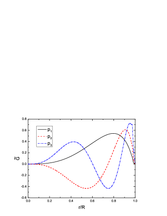
Figure 3: The scaled function $\tilde{G}_{n}$ of a NS with SLy EOS (Douchin & Haensel 2001, Haensel & Potekhin 2004) and compactness ${\cal C}=0.276$ is plotted against $r/R$ for $n=1$ (solid line), 2 (dashed line), 3 (dot-dashed line), which correspond to $p_{1}$, $p_{2}$ and $p_{3}$ modes, respectively.

C.3 Inverse-Cowling approximation

We can also obtain the ICA for polar $w$-modes within the F-S approach by neglecting the $F$ term in (21), i.e.,

$$\omega^{2}S+\frac{d^{2}S}{dr_{*}^{2}}+\frac{2e^{\nu}}{r^{3}}\left[2\pi r^{3}(\rho+3p)+m-(n+1)r\right]S=0.$$ (78)

Interestingly, such an ICA is merely the HFICA in the $H$-$S$ approach, which works well only for $w$-modes with high frequencies (see Table 5 for the accuracies and validity of HFICA in the $H$-$S$ approach). It reflects the fact that the metric variable $F$ also participates in the dynamics of stellar pulsations and its contribution to (21) is non-negligible for $w$-modes with low frequencies.

References

- (1)
- Allen et al. (1998) Allen, G., Andersson, N., Kokkotas, K. D., & Schutz, B. F. 1998, Phys. Rev. D, 58, 124012
- Andersson et al. (2011) Andersson, N., et al. 2011, Gen. Rel. Grav., 43, 409
- Andersson & Kokkotas (1996) Andersson, N., & Kokkotas, K. D. 1996, Phys. Rev. Lett, 77, 4134
- Andersson & Kokkotas (1998) —. 1998, MNRAS, 299, 1059
- Andersson et al. (1996) Andersson, N., Kokkotas, K. D., & Schutz, B. F. 1996, MNRAS, 280, 1230
- Benhar et al. (1999) Benhar, O., Berti, E., & Ferrari, V. 1999, MNRAS, 310, 797
- Benhar et al. (2004) Benhar, O., Ferrari, V., & Gualtieri, L. 2004, Phys. Rev. D, 70, 124015
- Berti et al. (2009) Berti, E., Cardoso, V., & Starinets, A. O. 2009, Class. Quant. Grav., 26, 163001
- Chandrasekhar & Ferrari (1991) Chandrasekhar, S., & Ferrari, V. 1991, Proc. R. Soc. Lond. A, 432, 247
- Ching et al. (1998) Ching, E. S. C., Leung, P. T., van den Brink, A. M., Suen, W. M., Tong, S. S., & Young, K. 1998, Rev. Mod. Phys., 70, 1545
- Cowling (1941) Cowling, T. G. 1941, MNRAS, 101, 367
- Detweiler & Lindblom (1985) Detweiler, S., & Lindblom, L. 1985, ApJ, 292, 12
- Doneva et al. (2013) Doneva D. D., Gaertig E., Kokkotas K. D., Krüger C., 2013, Phys. Rev. D, 88, 044052
- Douchin & Haensel (2001) Douchin, F., & Haensel, P. 2001, A&A, 380, 151
- Finn (1988) Finn L. S., 1988, MNRAS, 232, 259
- Fryer et al. (2002) Fryer, C. L., Holz, D. E., & Hughes, S. A. 2002, ApJ, 565, 430
- Glendenning (1997) Glendenning, N. K. 1997, Compact Stars - Nuclear Physics, Particle Physics, and General Relativity (Springer, NY)
- Haensel & Potekhin (2004) Haensel, P., & Potekhin, A. Y. 2004, A&A, 428, 191
- Hild et al. (2011) Hild, S., et al. 2011, Class. Quant. Grav., 28, 094013
- Hughes (2003) Hughes, S. 2003, Ann. Phys., 303, 142
- Kojima (1992) Kojima Y., 1992, Phys. Rev. D, 46, 4289
- Kokkotas et al. (2001) Kokkotas, K. D., Apostolatos, T. A., & Andersson, N. 2001, MNRAS, 320, 307
- Kokkotas & Schmidt (1999a) Kokkotas, K. D., & Schmidt, B. G. 1999a, Living Rev. Rel., 2, 2
- Konoplya & Zhidenko (2011) Konoplya R. A., Zhidenko A., 2011, Rev. Mod. Phys., 83, 793
- Lattimer & Prakash (2007) Lattimer, J., & Prakash, M. 2007, Phys. Rep., 442, 109
- Lattimer (2012) Lattimer J. M., 2012, Ann. Rev. Nucl. Part. Sci., 62, 485
- Lau et al. (2010) Lau, H. K., Leung, P. T., & Lin, L. M. 2010, ApJ, 714, 1234
- Leaver (1986) Leaver, E. W. 1986, Phys. Rev. D, 34, 384
- Lindblom & Detweiler (1983) Lindblom, L., & Detweiler, S. L. 1983, ApJ, 53, 73
- Lindblom et al. (1997) Lindblom, L., Mendell, G., & Ipser, J. R. 1997, Phys. Rev. D, 56, 2118
- Lindblom & Splinter (1990) Lindblom, L., & Splinter, R. J. 1990, ApJ, 348, 198
- McDermott et al. (1983) McDermott P. N., Horn H. M. V., Scholl J. F., 1983, ApJ, 268, 837
- Morse & Feshbach (1953) Morse, P. M., & Feshbach, H. 1953, Methods of Theoretical Physics, Part I (McGraw-Hill)
- Pandharipande (1971) Pandharipande, V. 1971, Nucl. Phys. A, 174, 641
- Press (1971) Press, W. 1971, ApJ, 170, L105
- Price & Thorne (1969) Price, R., & Thorne, K. S. 1969, ApJ, 155, 163
- Regge & Wheeler (1957) Regge, T., & Wheeler, J. A. 1957, Phys. Rev., 108, 1063
- Ruoff (2001) Ruoff, J. 2001, Phys. Rev. D, 63, 064018
- Sotani et al. (2011) Sotani, H., Yasutake, N., Maruyama, T., & Tatsumi, T. 2011, Phys. Rev. D, 83, 024014
- Thorne (1969) Thorne, K. S. 1969, ApJ, 158, 997
- Thorne & Campolattaro (1967) Thorne, K. S., & Campolattaro, A. 1967, ApJ, 149, 591
- Tsui & Leung (2005a) Tsui, L. K., & Leung, P. T. 2005a, Phys. Rev. Lett., 95, 151101
- Tsui & Leung (2005b) —. 2005b, ApJ, 631, 495
- Tsui et al. (2006) Tsui, L. K., Leung, P. T., & Wu, J. 2006, Phys. Rev. D, 74, 124025
- Weber (1999) Weber, F. 1999, Pulsars as Astrophysical Laboratories for Nuclear and Particle Physics (Institute of Physics Publishing)
- Wu & Leung (2007) Wu, J., & Leung, P. T. 2007, MNRAS, 381, 151
- Zerilli (1970) Zerilli, F. J. 1970, Phys. Rev. Lett., 24, 737
- Zettl (2005) Zettl, A. 2005, Sturm-Liouville Theory, Mathematical surveys and monographs (American Math. Soc.)
- Zhang et al. (2011) Zhang, Y. J., Wu, J., & Leung, P. T. 2011, Phys. Rev. D, 83, 064012