Radiating Kerr-Newman black hole in $f(R)$ gravity

Abstract

We derive an exact radiating Kerr-Newman like black hole solution, with constant curvature $R=R_{0}$ imposed, to metric $f(R)$ gravity via complex transformations suggested by Newman-Janis. This generates a geometry which is precisely that of radiating Kerr-Newman-de Sitter / anti-de Sitter with the $f(R)$ gravity contributing an $R_{0}$ cosmological-like term. The structure of three horizon-like surfaces, viz. timelike limit surface, apparent horizon and event horizon, are determined. We demonstrate the existence of an additional cosmological horizon, in $f(R)$ gravity model, apart from the regular black hole horizons that exist in the analogous general relativity case. In particular, the known stationary Kerr-Newman black hole solutions of $f(R)$ gravity and general relativity are retrieved. We find that the timelike limit surface becomes less prolate with $R_{0}$ thereby affecting the shape of the corresponding ergosphere.

I Introduction

The $f(R)$ gravity, where $f(R)$ is an analytic function of the Ricci scalar $R$, comes into existence as a straightforward extension of general relativity (GR) frr ; frr1 ; scml . In these theories the curvature scalar $R$ of the Lagrangian in the Einstein-Hilbert action is replaced by an arbitrary function of the curvature scalar thereby modifying GR. However, the $f(R)$ action is sufficiently general to encapsulate some of the basic characteristics of higher order gravity. It is an interesting and relatively simple alternative to GR, the study of which yields useful conclusions frr ; frr1 ; scml , including the present day acceleration. Unlike GR, which demands metric function derivatives no higher than second order, the metric $f(R)$ gravity has up to fourth order derivatives lc . This causes complication in the calculations and hence, in general, finding exact solutions in this theory is laborious. Accordingly, little is known about $f(R)$ gravity exact solutions, which deserve to be understood better. Nevertheless, recently, interesting measures have been taken to get the spherically symmetric solutions of $f(R)$ gravity mv ; cen ; cdm ; sz ; pbon ; asav ; Moon ; ncgd ; cst08 . In particular, spherically symmetric black hole (BH) solutions were obtained for a positive constant curvature scalar in cen , and a BH solution was obtained in $f(R)$ gravities by requiring the presence of a negative constant curvature scalar cdm . Also, several spherical $f(R)$ BH solutions have been obtained cdm ; sz ; pbon ; asav ; Moon . The generalization of these stationary $f(R)$ BHs to the axially symmetric case, Kerr-Newman BH, was addressed recently cls ; cdr ; al ; adds . In particular, it is demonstrated cls that the rotating BH solutions for $f(R)$ gravity can be derived starting from exact spherically symmetric solutions by a complex coordinate transformation previously developed by Newman and Janis nj in GR. However, the axially symmetric $f(R)$ is still unexplored, e.g., the radiating generalization of the $f(R)$ Kerr-Newman BH is still unknown. It is the purpose of this paper to generate this metric and we also present the $D$-dimensional Kerr metric in $f(R)$ gravity. Thus we extend a recent work of ours sgsd on radiating $f(R)$ BH to include rotation. The Kerr metric kerr is undoubtedly the single most significant exact solution in the Einstein theory of GR, which represents the prototypical BH that can arise from gravitational collapse. The Kerr-Newman spacetime is associated with the exterior geometry of a rotating massive and charged BH ggsh . It is well known that Kerr BH enjoys many interesting properties distinct from its nonspinning counterpart, i.e., from Schwarzschild BH. However, there is a surprising connection between the two BHs of Einstein theory, and was analysed by Newman and Janis nja . They demonstrated that applying a complex coordinate transformation, it was possible to construct both the Kerr and Kerr-Newman solutions starting from the Schwarzschild metric and Reissner Nordstr$\ddot{o}$m, respectively nja . For a review on the Newman-Janis algorithm see, e.g., d'Inverno .

In this paper, the Newman-Janis algorithm is applied to spherically symmetric radiating $f(R)$ BH solutions, and the corresponding radiating rotating solutions, namely radiating $f(R)$ Kerr-Newman metrics are obtained in Section III. We investigate further the structure and location of horizons of the radiating $f(R)$ Kerr-Newman metric in Section IV. We consider whether $f(R)$ gravity plays any special role in the formation of horizons in Section V. The general remarks on $f(R)$ gravity is given in Section II, and here we also discuss briefly basic equations of HD $f(R)$ gravity. The paper ends with concluding remarks in Section VI. We also give the HD Kerr like metric, for constant curvature imposed, $f(R)$ gravity, in the appendix. We use units which fix the speed of light and the gravitational constant via $G=c=1$, and use the metric signature ($+,\;-,\;-,\;-$).

II Basic Equations of Metric $f(R)$ gravity

In this section we briefly review the metric $f(R)$ gravity in higher-dimensional (HD) spacetime. The starting point is the modified Einstein-Hilbert, $D$-dimensional, gravitational action cdm :

$$I=\frac{1}{16\pi}\int{d}^{D}x\sqrt{-g}\,(R+f(R)),$$ (1)

where $g$ is the determinant of the metric $g_{ab}$, $(a,b=0,1,...,D-1)$, $R$ is the scalar curvature, and $f(R)$ is the real function defining the theory under consideration. As the simplest example, the Einstein-Hilbert action with cosmological constant $\Lambda_{f}$ is given by $f(R)=-(D-2)\Lambda_{f}$.

From the above action, the equations of motion in the metric formalism are just scml :

$$R_{ab}(1+f^{\prime}(R))-\frac{1}{2}(R+f(R))\,g_{ab}$$

$$+ (g_{ab}\nabla^{2}-\nabla_{a}\nabla_{b})f^{\prime}(R)=2T_{ab},$$ (2)

where $R_{ab}$ is the usual Ricci tensor, the prime in $f^{\prime}(R)$ denotes differentiation with respect to $R$, and $\nabla^{2}=\nabla_{a}\nabla^{a}$ with $\nabla$ being the usual covariant derivative. Here, we are interested in obtaining the constant scalar curvature solutions $R\,=\,R_{0}$. Taking the trace in the Eq. (2), we get

$$2(1+f^{\prime}(R_{0}))\,R_{0}-D\,(R_{0}+f(R_{0}))\,=\,0,$$ (3)

where we assume that $T=T^{a}_{a}=0$ and note that $g_{a}^{a}=\delta^{a}_{a}=D$. Eq.  (3) determines the negative constant curvature scalar as cdm

$$R_{0}=\frac{D\,f(R_{0})}{2(1+f^{\prime}(R_{0}))-D}\equiv D\Lambda_{f}.$$ (4)

Thus any constant curvature solution $R=R_{0}$ with $1+f^{\prime}(R_{0})\neq 0$ obeys scml

$$R_{ab}=\Lambda_{f}g_{ab}+\frac{2}{1+f^{\prime}(R_{0})}T_{ab}.$$ (5)

For this kind of solution an effective cosmological constant may be defined as $\Lambda_{f}\equiv R_{0}/D$ for $D$-dimensional spacetime. In this paper we consider the case with conformal matter ($T=T_{a}^{a}=0$). For the case of conformal matter with non-vanishing $\Lambda_{f}$ we have again constant $R=R_{0}$ with $R_{0}=D\Lambda_{f}$ and $g_{ab}$ is a solution of $f(R)$ provided that once again $f(D\Lambda_{D})=\Lambda_{D}(2-D+2f^{\prime}D\Lambda_{D})$. In this case the solution is dS or (A)dS depending on the sign of $R_{0}$, just as in GR with a cosmological constant.

We note that the condition $1+f^{\prime}(R_{0})>0$ is required to avoid the appearance of ghosts frr , and a necessary condition that the stationary $f(R)$ BH becomes a type of Schwarzschild-(A)dS BH. Further, we require that $f^{\prime\prime}(R)>0$ to avoid the negative mass squared of a scalar-field degree of freedom, i.e., to avoid a tachyonic instability frr ; lc . Also $f(R)$ is a monotonic increasing function with $-1<f^{\prime}(R)<0.$

III Radiating Rotating $f(R)$ BH via Newman-Janis

Let us begin with the action for $f(R)$ gravity with a Maxwell term in the 4D case Moon :

$$I_{g}=\frac{1}{16\pi}\int d^{4}x\sqrt{-g}\Big{[}R+f(R)-F_{ab}F^{ab}\Big{]}.$$ (6)

The Maxwell tensor is $F_{ab}=\partial_{a}A_{b}-\partial_{b}A_{a}$, where $A_{a}$ is the vector potential. From the variation of the above action (6), the Einstein equation of motion can be written as cdm ; Moon

$$R_{ab}\Big{(}1+f^{\prime}(R)\Big{)}-\frac{1}{2}\Big{(}R+f(R)\Big{)}g_{ab}$$

$$+\Big{(}g_{ab}\nabla^{2}-\nabla_{a}\nabla_{b}\Big{)}f^{\prime}(R)=2T_{ab}^{EM},$$ (7)

with the EMT for charged null dust dg

$$T_{ab}^{EM}=\zeta(v,r)n_{a}n_{b}+F_{a\rho}F_{b}~{}^{\rho}-\frac{g_{ab}}{4}F_{\rho\sigma}F^{\rho\sigma}.$$ (8)

Once again, it is easy to see that the trace of the EMT is $T^{EM}=0$, due to the fact that $F^{a}_{a}=0$ in 4D. However, in HD $T^{EM}\neq 0$. On the other hand, the Maxwell equations take the form $\nabla_{a}F^{ab}=0.$ To proceed further, with constant curvature constant $R_{0}$, and taking the trace of the Eq. (III), after some algebra, leads to

$$R_{0}=\frac{2f(R_{0})}{f^{\prime}(R_{0})-1}\equiv 4\Lambda_{f}.$$ (9)

Thus any constant curvature solution $R=R_{0}$ obeys

$$R_{ab}=\Lambda_{f}g_{ab}+\frac{2}{1+f^{\prime}(R_{0})}T_{ab},$$ (10)

and an effective cosmological constant may be defined as $\Lambda_{f}\equiv R_{0}/4$.

Here we wish to obtain general $f(R)$ radiating rotating BH solution from a spherically symmetric BH solution via the complex transformation suggested by Newman-Janis nja . For this purpose, We begin with the “seed metric”, expressed in terms of the Eddington (ingoing) coordinate $v$, as:

$$ds^{2}=e^{\psi(v,r)}dv\left[f(v,r)e^{\psi(v,r)}dv+2dr\right]-r^{2}d\Omega^{2},$$ (11)

with $d\Omega^{2}=d\theta^{2}+\sin^{2}\theta d\phi^{2}$. Here $e^{\psi(v,r)}$ is an arbitrary function. It is useful to introduce a local mass function $m(v,r)$ defined by $f(v,r)=1-{2m(v,r)}/{r}$. For $m(v,r)=M(v)$ and $\psi(v,r)=0$, the metric reduces to the standard Vaidya metric. We can always set without any loss of generality, $\psi(v,r)=0.$ Thus any spherically symmetric radiating BH is defined by the metric (11). The function $f(v,r)$ is a function of $v$ and $r$, and depends on the matter field and the underlying theory and on functional form of $f(R)$ and Ricci curvature scalar $R=R(v,r)$.

The Newman-Janis algorithm can be applied to any spherically symmetric static solution, generating rotating spacetimes nj . For example, The Kerr metric can be obtained from the Schwarzschild metric, and Reissner-Nordstr$\ddot{o}$m solution leads to the Kerr-Newman solutions nj ; d'Inverno which is based on a complex coordinate transformation. Recently, the axially symmetric model for $f(R)$-gravity is derived from exact spherically symmetric $f(R)$-gravity solutions cls ; Mdl . In the following, we apply the Newman-Janis algorithm to the general spherically symmetric radiating BH given by Eq. (11) in order to construct a general radiating rotating BH solution.

The metric $\tilde{g}_{ab}$ given by Eq. (11) can be written in terms of a null tetrad nja ; cls as:

$$\tilde{g}^{ab}=-L^{a}N^{b}-L^{b}N^{a}+M^{a}\bar{M}^{b}+M^{b}\bar{M}^{a}$$ (12)

This tetrad is orthonormal obeying the conditions

$$L_{a}M^{a}=L_{a}\bar{M}^{a}=N_{a}M^{a}=N_{a}\bar{M}^{a}=0,$$ (13)

$$L_{a}L^{a}=N_{a}N^{a}=M_{a}M^{a}=\bar{M}_{a}\bar{M}^{a}=0,$$ (14)

$$L_{a}N^{a}=-1,~{}~{}~{}M_{a}\bar{M}^{a}=1.$$ (15)

Next, we perform the similar complex coordinate transformation as used by Newman and Janis nja :

$${x^{\prime}}^{\mu}=x^{\mu}+ia(\delta_{r}^{\mu}-\delta_{u}^{\mu})\cos\theta\rightarrow\\ \left\{\begin{array}[]{ll}v^{\prime}=v-ia\cos\theta,\\ r^{\prime}=r+ia\cos\theta,\\ \theta^{\prime}=\theta,~{}~{}~{}\phi^{\prime}=\phi.\end{array}\right.$$ (16)

and also transform the tetrad $Z^{a}_{s}=(L^{a},\;N^{a},\;M^{a},\;\bar{M}^{a})$ in the usual way

$$Z^{\prime a}_{s}=\frac{\partial x^{\prime a}}{\partial x^{b}}Z^{b}_{s},$$ (17)

which leads to

$$L^{a} = \delta^{a}_{r},$$ (18)

$$N^{a} = \left[\delta^{a}_{v}-\frac{1}{2}f(v,r)\delta^{a}_{r}\right],$$ (19)

$$M^{a} = \frac{1}{\sqrt{2}r}\left[ia\sin\theta\left(\delta^{a}_{v}-\delta^{a}_{r}\right)+\delta^{a}_{\theta}+\frac{i}{\sin\theta}\delta^{a}_{\phi}\right],$$ (20)

$$\bar{M}^{a} = \frac{1}{\sqrt{2}\bar{r}}\left[-ia\sin\theta\left(\delta^{a}_{v}-\delta^{a}_{r}\right)+\delta^{a}_{\theta}-\frac{i}{\sin\theta}\delta^{a}_{\phi}\right],$$ (21)

and, we have dropped the primes. This transformed tetrad yields a new metric given by the line element (see Ref. nja ; cls , for further details):

$$ds^{2} = \mathcal{F}(v,r,\theta)dv^{2}-\Sigma(r,\theta)d\theta^{2}+2\;[dv-a\sin^{2}\theta d\phi]\;dr$$ (22)

$$- \left[a^{2}(2-\mathcal{F}(v,r,\theta))\sin^{2}\theta+\Sigma(r,\theta)\right]\sin^{2}\theta d\phi^{2}$$

$$+ 2a\left[1-\mathcal{F}(v,r,\theta)\right]\sin^{2}\theta dv\;d\phi.$$

Here $\mathcal{F}(v,r,\theta)$ is function which depends on $f(r,v)$, e.g., for the function $f(v,r)=1-\frac{2M(v)}{r}+\frac{2\tilde{Q}^{2}(v)}{r^{2}}$, it has the form $\mathcal{F}(v,r,\theta)=1-\frac{2M(v)r}{\Sigma}+\frac{2\tilde{Q}^{2}(v)}{\Sigma}$, where $\Sigma\equiv r^{2}+a^{2}\cos^{2}\theta$.

The spherically symmetric collapsing solution of the $f(R)$ gravity can be classified according to choice of the Ricci curvature scml . The prototype of general pure $f(R)$ gravity (nonconstant curvature) are the models viz. $f(R)=R-\mu^{4}/R$, $f(R)=R+\kappa R^{n}$, $f(R)=R-\lambda\exp(-\zeta R)$, $f(R)=R-\lambda\exp(-\zeta R)+\kappa R^{2}$ and $f(R)=R-\lambda\exp(-\zeta R)+\kappa R^{n}+\eta\ln R$, where $\mu,\;\kappa,\;\lambda,\;\zeta$ and $\eta$ are some constants scml . Hendi et al. shh obtained static solutions for these choices of $f(R)$ in the pure $f(R)$-gravity and demonstrated that starting from pure $f(R)$ gravity, with above mentioned choice of $f(R)$, leads to (charged) Einstein-$\Lambda$ solutions which can be interpreted as (charged) (a)dS BH solutions shh . Following shh , we find the corresponding radiating solution up&sgg and it turns out that the solution is given by the metric  (11), with

$$f(v,r)=\kappa-\frac{2M(v)}{r}+\frac{2\tilde{Q}^{2}(v)}{r^{2}}-\frac{\Lambda}{3}r^{2},$$ (23)

where $M(v)$ and $\tilde{Q}(v)$ are functions of integration and $\Lambda$ may be interpreted as the cosmological constant emerging from $f(R)$ gravity and we choose $\Lambda=R_{0}/4$ and also $\kappa=1$. The function $\tilde{Q}(v)$ can be zero for some choice of $f(R)$, i.e., for the model $f(R)=R+\kappa R^{n}$, we cannot obtain charged solutions, i.e., in this case the solution  (23) is valid with $\tilde{Q}(v)=0$. Thus it is clear that the general radiating spherically symmetric solution in several $f(R)$ gravity models, with the choice of $f(R)$ mentioned above, result to the metric (11) with $f(v,r)$ as (23).

Now we start with the radiating spherically symmetric metric (11), written in Eddington-Finkelstein coordinate, with $f(v,r)$ as given by (23). By performing the Newman-Janis algorithm, we derive the $f(R)$ radiating rotating solution which takes the form:

$$ds^{2} = \frac{A}{\Sigma}\left[\Delta-\Theta a^{2}\sin^{2}\theta\right]dv^{2}+2\sqrt{A}\left[dv-a\sin^{2}d\phi\right]dr$$ (24)

$$-\frac{\Sigma}{\Theta}d\theta^{2}+A\frac{2a}{\Sigma}\left[\Delta(r^{2}+a^{2})-\Theta\right]\sin^{2}\theta dvd\phi$$

$$-\frac{A}{\Sigma}\left[\Delta(r^{2}+a^{2})^{2}-\Theta a^{2}\sin^{2}\theta\right]\sin^{2}\theta d\phi^{2},$$

where

$$\Sigma^{2} = r^{2}+a^{2}\cos^{2}\theta,$$

$$\Delta = r^{2}+a^{2}-2M(v)r+\tilde{Q}^{2}(v)-\frac{R_{0}r^{2}}{12}(r^{2}+a^{2}),$$

$$\Theta = 1+\frac{R_{0}}{12}a^{2}\cos^{2}\theta,$$

$$A = \left(1+\frac{R_{0}}{12}a^{2}\right)^{-2},$$

$$\tilde{Q}^{2}(v) = \frac{2{Q}^{2}(v)}{1+f^{\prime}(R_{0})},$$

and the related electromagnetic potential is

$$A_{a}=\frac{\tilde{Q}(v)r}{\Sigma^{2}}\left[\sqrt{A},\;0,\;0,\;-\sqrt{A}a\sin^{2}\theta\right].$$ (25)

Here $M(v)$ and $\tilde{Q}(v)$ are functions of retarded time $v$ identified, respectively, as mass and charge of spacetime, and $a$ is the angular momentum per unit mass. We have applied the aforesaid procedure to a class of $f(R)$ gravity radiating models. But, the method is general and is applicable to any general radiating spherically symmetric solution in $f(R)$ gravity. It describes the exterior field of the radiating rotating charged body. Thus we have a kind of charged radiating rotating metric in de Sitter/ anti-de Sitter (dS/AdS) like spacetime or radiating Kerr-Newman dS / AdS like solution. The stationary $f(R)$ Kerr-Newman BH cdr ; al ; adds in $(t,\;r,\;\theta,\;\phi)$ can be obtained by means of the local coordinate transformation and replacing $M(v)$ and $\tilde{Q}(v)$ by constants $M$ and $Q$. The metric (24) of radiating $f(R)$ Kerr-Newman BH is a natural generalization of the stationary Kerr-Newman BH solutions of $f(R)$ gravity cdr ; al , but it is Petrov type-II, whereas the latter is of Petrov type-D. In addition, if $R_{0}=0$ then metric (24) makes the Kerr-Newman metric. Hence, we refer to the solution as a radiating $f(R)$ Kerr-Newman solution representing gravitational collapse of a charged null fluid in a non-flat dS/AdS like spacetime. Thus, the metric (24) bears the same relation to Kerr-Newman as does Vaidya metric to Schwarzschild metric. Also for $Q=0$, the metric (24) is radiating $f(R)$ Kerr spacetime al ; cdr . If in addition $R_{0}\rightarrow 0$, we have Kerr spacetime and for $a\rightarrow 0$ the metric (24) is $f(R)$ Bonnor-Vaidya spacetime which has zero angular momentum sgsd . The radiating rotating charged solution discussed here is derived under the assumption of the constant curvature $R=R_{0}$, in which case the $f(R)$ models are equivalent to GR and a cosmological constant, and also the solution is time-dependent.

IV Singularity and physical parameters of radiating $f(R)$ Kerr-Newman BH

The metric of the radiating $f(R)$ Kerr-Newman BH solution has the form (24) with electromagnetic potential given by (25) and the energy momentum tensor (8). Here, we shall discuss the singularity structure of radiating $f(R)$ Kerr-Newman BH derived in the previous section. The easiest way to detect a singularity in a spacetime is to observe the divergence of some invariants of the Riemann tensor. We approach the singularity problem by studying the behaviour of the Ricci $\mbox{R}=R_{ab}R^{ab}$, ($R_{ab}$ the Ricci tensor) and Kretschmann invariants $\mbox{K}=R_{abcd}R^{abcd}$, ($R_{abcd}$ the Riemann tensor). For the metric (24) they behave as:-

$$\mbox{R}\approx\frac{\mathcal{F}\left(\tilde{Q}(v),R_{0}\right)}{(r^{2}+a^{2}\cos^{2}\theta)^{4}},$$

$$\mbox{K}\approx\frac{\mathcal{G}\left(M(v),\;\tilde{Q}(v),\;a,\;\cos\theta,\;R_{0}\right)}{(r^{2}+a^{2}\cos^{2}\theta)^{6}},$$ (26)

where $\mathcal{F}$ and $\mathcal{G}$ are some functions. It is sufficient to study the Kretschmann and Ricci scalars for the investigation of the spacetime curvature singularity(ies). These invariants are regular everywhere except at the origin $r=0$ but only at the equatorial plane $\theta=\pi/2$ for $a,\;M(v),\;$ and $\tilde{Q}(v)\neq 0$. Hence, the spacetime has the scalar polynomial singularity he at $r=0$. The study of causal structure of the spacetime is beyond the scope of this paper and will be discussed elsewhere.

In order to further discuss the physical nature of radiating $f(R)$ Kerr-Newman BH, we introduce their kinematical parameters. Following bc ; jy ; rm ; bdk ; xd98 ; xd99 , the null-tetrad of the metric (24) is of the form

$$l_{a} = \left[\sqrt{A},\;0,\;0,\;-\sqrt{A}a\sin^{2}\theta\right],$$

$$n_{a} = \left[\sqrt{A}\frac{\Delta}{2\Sigma},\;1,\;0,\;\sqrt{A}\frac{\Delta}{2\Sigma}a\sin^{2}\theta\right],$$

$$m_{a} = \frac{\sigma}{\sqrt{2}\rho}\left[\sqrt{A}ia\sin\theta,\;0,\;\frac{\Sigma}{\Theta},\;-\sqrt{A}i(r^{2}+a^{2})\sin\theta\right],$$

$$\bar{m}_{a} = \frac{\bar{\sigma}}{\sqrt{2}\bar{\rho}}\left[-\sqrt{A}ia\sin\theta,\;0,\;\frac{\Sigma}{\Theta},\;\sqrt{A}i(r^{2}+a^{2})\sin\theta\right],$$

where

$$\rho = r+ia\cos\theta,$$

$$\sigma = 1+i\sqrt{\left(\frac{R_{0}}{12}\right)}a\cos\theta,$$

and $\bar{\rho}$ and $\bar{\sigma}$ are complex conjugates of, respectively, $\rho$ and $\sigma$. The null tetrad obeys null, orthogonal and metric conditions

$$l_{a}l^{a} = n_{a}n^{a}=m_{a}m^{a}=0,\;~{}l_{a}n^{a}=1,$$

$$l_{a}m^{a} = n_{a}m^{a}=0,\;m_{a}\bar{m}^{a}=-1,$$

$$g_{ab} = l_{a}n_{b}+l_{b}n_{a}-m_{a}\bar{m}_{b}-m_{b}\bar{m}_{a},$$

$$g^{ab} = l^{a}n^{b}+l^{b}n^{a}-m^{a}\bar{m}^{b}-m^{b}\bar{m}^{a}.$$ (27)

Inspired by the arguments in Ref. bc ; jy , a null-vector decomposition of the $f(R)$-metric (24) is of the form

$$g_{ab}=-n_{a}l_{b}-l_{a}n_{b}+\gamma_{ab},$$ (28)

where $\gamma_{ab}=m_{a}\bar{m}_{b}+m_{b}\bar{m}_{a}$. Next we construct all physical parameters which help us to discuss the horizon structure of radiating $f(R)$ Kerr-Newman BH. The optical behavior of null geodesics congruences is governed by the Raychaudhuri equation jy ; rm ; bdk ; xd98 ; xd99 .

$$\frac{d\Theta}{dv}=\kappa\Theta-R_{ab}l^{a}l^{b}-\frac{1}{2}\Theta^{2}-\sigma_{ab}\sigma^{ab}+\omega_{ab}\omega^{ab},$$ (29)

with expansion $\Theta$, twist $\omega$, shear $\sigma$, and surface gravity $\kappa$. The expansion jy of the null rays, parameterized by $v$, is given by

$$\Theta=\nabla_{a}l^{a}-\kappa,$$ (30)

where $\nabla$ is the covariant derivative. In the present case, the surface gravity jy is

$$\kappa=-n^{a}l^{b}\nabla_{b}l_{a},$$ (31)

and the shear jy takes form

$$\sigma_{ab}=\Theta_{ab}-\Theta(\gamma_{c}^{c})\gamma_{ab}.$$ (32)

The luminosity due to loss of mass is given by $L_{M}=-dM/dv$, $L_{M}<1$ , and due to gauge charge by $L_{Q}=-dQ/dv$, where $L_{M},L_{Q}<1$. Both are measured in the region where $d/dv$ is timelike jy ; rm ; bdk .

V Three kinds of horizons

If one considers $f(R)$ theory as modification of GR, it is natural to discuss not only BH solutions but it’s various properties in this theory. It is expected that some features of BH may get modified in $f(R)$ theories. In this section we explore horizons of radiating $f(R)$ Kerr-Newman BH, discuss the effects which come from the $f(R)$ theories. A BH has three horizon-like surfaces jy : timelike limit surface (TLS), apparent horizon (AH) and event horizon (EH). For a classical Schwarzschild BH (which does not radiate), the three surfaces EH, AH and TLS are all identical. Upon switching on the Hawking evaporation this degeneracy is partially lifted even if the spherical symmetry stays, e.g., for Vaidya radiating BH, we have then AH=TLS, but the EH is different If we break spherical symmetry preserving stationarity (e.g., Kerr BH), then AH=EH but EH $\neq$ TLS. In general, e.g., for radiating Kerr-Newman BH, the three surfaces AH $\neq$ TLS $\neq$ EH and they are sensitive to small perturbations.

Here we are interested in these horizons for the radiating $f(R)$ Kerr-Newman BH. As demonstrated first by York jy , the horizons may be obtained to $O(L_{M},L_{Q})$ by noting that (i) for a BH with small dimensionless accretion, we can define TLS’s as locus where $g(\partial_{v},\partial_{v})=g_{vv}=0$ (ii) AHs are defined as surface such that $\Theta\simeq 0$ and (iii) EHs are surfaces such that $d\Theta/dv\simeq 0$.

Figure 1: TLS of radiating $f(R)$ Kerr-Newman BH: Plots showing positive roots of Eq. (V.1) which corresponds TLS of radiating Kerr-Newman BH for $M(v)=\lambda v+O(v)$ and $\tilde{Q}(v)=\mu^{2}v^{2}+O(v^{2})$ with parameters values $\lambda=0.04,\;\mu=0.08$,  and $\theta=0.3$. The three roots corresponds to $r_{TLS}^{-}$ (inner) and $r_{TLS}^{+}$ (outer), and $r_{dTLS}$ of radiating $f(R)$ Kerr-Newman BH. LEFT: For different values of $R_{0}$ with $a=0.3$. RIGHT: For different values of $a$ with $R_{0}=0.5$.

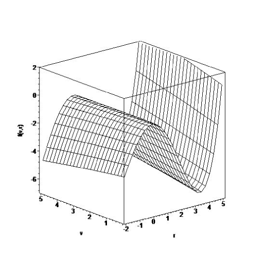
Figure 2: A plot of the function $\mathfrak{f}(v,r,\theta)$ for $M(v)=\lambda v+O(v)$ and $\tilde{Q}(v)=\mu^{2}v^{2}+O(v^{2})$ with parameters values $\lambda=0.04,\;\mu=0.08,\;\theta=0.3,\ a=0.7$ and $R_{0}=0.3$. The zeros of $\mathfrak{f}(v,r,\theta)=0$ determines the TLS of radiating $f(R)$ Kerr-Newman BH

V.1 Time-like limit surface

The TLS is defined as the surface where the static observer become light-like and it can be null, timelike or spacelike jy . First, we calculate the location of TLS surface, which for the nonstationary radiating $f(R)$ Kerr-Newman metric requires that prefactor of the $dv^{2}$ term in metric vanishes; It follows from Eq. (24) that TLS will satisfy xd99

$$\Delta_{r}-\Delta_{\theta}a^{2}\sin^{2}\theta=0.$$ (33)

This equation can be rewritten as

$$\mathfrak{f}(v,r,\theta)=\frac{R_{0}}{12}r^{4}-\left(1-\frac{R_{0}a^{2}}{12}\right)r^{2}+2M(v)r$$

$$+\frac{R_{0}}{12}\cos^{2}\theta\sin^{2}\theta a^{4}-\cos\theta^{2}a^{2}-\tilde{Q}^{2}(v)=0,$$ (34)

Equation (V.1) is a reduced quartic equation. It is easy to check, under condition of the discriminant in cond , Eq. (V.1) admits four real roots. For positive curvature $R_{0}>0$, Eq. (V.1), subject to restriction cond , has all four real roots with three positive and one negative. In the Fig. 1, we show three positive roots of the Eq. (V.1). The other three positive roots corresponds to $r_{TLS}^{-}$ (inner) and $r_{TLS}^{+}$ (outer), and $r_{dTLS}$ (dS-like TLS). Clearly, $r_{TLS}^{-}\;<\;r_{TLS}^{+}\;<\;r_{dTLS}$ and that $r_{TLS}^{-}$ and $r_{TLS}^{+}$ are TLSs of a BH, whereas the root $r_{dTLS}$ is supplementary TLS due to the $f(R)$ gravity term. When $R_{0}=0$, i.e., in GR limit, have just two outer and inner TLSs of radiating Kerr-Newman BH.

As mentioned above, in the limit $a\rightarrow 0$, one gets $f(R)$ Bonnor-Vaidya solution sgsd , and Eq. (V.1) takes the form

$$\frac{R_{0}}{12}r^{4}-r^{2}+2M(v)r-\tilde{Q}^{2}(v)=0.$$ (35)

This coincides with the nonrotational case in which case the various horizons are identified and analyzed by us in sgsd and hence, to conserve space, we shall avoid the repetition of same. Further, in the GR limit $R_{0}\rightarrow 0;\tilde{Q}(v)\rightarrow Q(v)$, we obtain

$${r}^{2}+\cos^{2}\left(\theta\right){a}^{2}-2\,M\left(v\right)r+Q^{2}\left(v\right)=0,$$ (36)

which trivially solves to

$$r_{TLS}^{-} = M(v)-\sqrt{M^{2}(v)-{a}^{2}\cos^{2}\theta-Q^{2}(v)},$$

$$r_{TLS}^{+} = M(v)+\sqrt{M^{2}(v)-{a}^{2}\cos^{2}\theta-Q^{2}(v)}.$$ (37)

These are regular outer and inner TLSs for a radiating Kerr-Newman BH ggsh , and further in the non-rotating limit $a\rightarrow 0$, the solutions (V.1) reduces to

$$r_{TLS}^{-} = M(v)-\sqrt{M^{2}(v)-Q^{2}(v)},$$

$$r_{TLS}^{+} = M(v)+\sqrt{M^{2}(v)-Q^{2}(v)},$$ (38)

which are TLS of Bonnor-Vaidya BH. Thus the radiating $f(R)$ Kerr-Newman BH, in the GR limit and $a\rightarrow 0$, degenerates to Bonnor-Vaidya BH dg .

The TLSs of radiating $f(R)$-Kerr-Newman BH is shown in Fig. 1 for different values of the parameter $R_{0}$ and rotation parameter $a$ and surface plot in Fig. 2 shows the TLSs for the variable time $v$. In Fig. 3, we compared the TLSs and AHs for different values of rotation parameter of radiating Kerr-Newman BH. For the definiteness we choose $M(v)=\lambda v+O(v)$ and $\tilde{Q}(v)=\mu^{2}v^{2}+O(v^{2})$.

V.2 Apparent Horizon

Figure 3: Plots showing the comparison of AH and TLS for radiating Kerr Newman BH $(R_{0}=0)$ choosing $M(v)=\lambda v+O(v)$ and $\tilde{Q}(v)=\mu^{2}v^{2}+O(v^{2})$ with parameter values $\lambda=0.04$, $\mu=0.08$ for different values of rotation parameter $a=0.2,0.4,0.6,0.7$.

The AH is the outermost marginally trapped surface for the outgoing photons. The AH can be either null or spacelike, that is, it can ‘move’ causally or acausally jy . The AHs are defined as surfaces such that $\Theta\simeq 0$ jy . Eqs. (IV) and (31) give the expression for surface gravity

$$\kappa=\frac{1}{2\Sigma}\left[\frac{\partial\Delta_{r}}{\partial r}-\frac{2r}{\Sigma}\Delta_{r}\right],$$ (39)

which on inserting the expression for $\Delta_{r}$, becomes

$$\kappa = \frac{R_{0}}{12\Sigma^{2}}-\left(\frac{R_{0}}{6\Sigma}-\frac{1-\frac{R_{0}a^{2}}{12}}{\Sigma^{2}}\right)r^{3}+\frac{2M(v)}{\Sigma^{2}}r^{2}$$ (40)

$$+\left(\frac{1-\frac{R_{0}a^{2}}{12}}{\Sigma}-\frac{a^{2}+\tilde{Q}^{2}(v)}{\Sigma^{2}}\right)r-\frac{M(v)}{\Sigma}.$$

Eqs. (IV), (30) and (39) then yield

$$\Theta = -\frac{r}{\Sigma^{2}}\Delta_{r}=\frac{r}{\Sigma^{2}}\Big{[}\frac{R_{0}}{12}r^{4}-\left(1-\frac{R_{0}a^{2}}{12}\right)r^{2}$$ (41)

$$+2M(v)r-\left(a^{2}+\tilde{Q}^{2}(v)\right)\Big{]}.$$

It is evident that the AHs are zeros of $\Theta=0$. From Eq. (41), thus the AH’s are given by zeros of

$$g(v,r) = \frac{R_{0}}{12}r^{4}-\left(1-\frac{R_{0}a^{2}}{12}\right)r^{2}+2M(v)r$$ (42)

$$-\left(a^{2}+\tilde{Q}^{2}(v)\right)=0.$$

Again in GR limit, we get

$$r^{2}-2M(v)r+\left(a^{2}+{Q}^{2}(v)\right)=0,$$ (43)

which admit solutions

$$r_{AH}^{-} = M(v)-\sqrt{M^{2}(v)-{a}^{2}-Q^{2}(v)},$$

$$r_{AH}^{+} = M(v)+\sqrt{M^{2}(v)-{a}^{2}-Q^{2}(v)}.$$ (44)

Figure 4: AH of radiating $f(R)$ Kerr-Newman BH: Plots showing positive roots of Eq. (42) which corresponds AH of radiating Kerr-Newman BH for $M(v)=\lambda v+O(v)$ and $\tilde{Q}(v)=\mu^{2}v^{2}+O(v^{2})$ with parameters values $\lambda=0.04,\;\mu=0.08$,  and $\theta=0.3$. The three roots corresponds to $r_{AH}^{-}$ (inner) and $r_{AH}^{+}$ (outer), and $r_{dAH}$ of radiating $f(R)$ Kerr-Newman BH. LEFT: For different values of $R_{0}$ with $a=0.3$. RIGHT: For different values of $a$ with $R_{0}=0.5$.

There exist, subject to condition cond , three positive roots for $R_{0}>0$ as shown in the Figs. 4 and 5. Unlike, TLS, the AH’s are $\theta$ independent. Hence, unlike non-rotating BHs, they do not coincide in the rotating case. The three roots correspond to inner and outer BH AHs, and dS-like AH. The structure of the AH is depicted in the Fig. 4. The surface plot in Fig. 5 shows AH for different values of rotation parameter $a$ and time $v$ of radiating $f(R)$-Kerr-Newman BH. For the definiteness we choose $M(v)=\lambda v+O(v)$ and $\tilde{Q}(v)=\mu^{2}v^{2}+O(v^{2})$.

These are regular outer and inner AHs for a radiating Kerr-Newman BH, and further in the non-rotating limit $a\rightarrow 0$, the solutions (V.2) correspond to Bonnor-Vaidya AHs. Further, Eq. (V.2) in the limit $a\rightarrow 0$ becomes exactly Eq. (V.1). Thus AHs coincide with TLSs, for the non-rotating but radiating, Bonnor-Vaidya case sgsd .

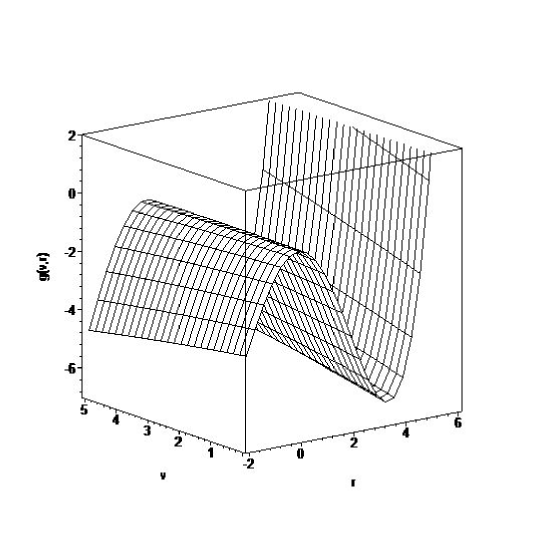
Figure 5: A plot of the function $g(v,r)$ for $M(v)=\lambda v+O(v)$ and $\tilde{Q}(v)=\mu^{2}v^{2}+O(v^{2})$ with parameters values $\lambda=0.04,\;\mu=0.08,\;\theta=0.3$ and $R_{0}=0.5$

.

The discussion in above two subsections are also valid for the stationary case discussed in cdr . In the stationary case $M$ and $Q$ are constant whereas in the radiating case $M(v)$ and $\tilde{Q}(v)$ are function of the retarded time $v$. Thus, Eqs. (V.1) and (42) are the same as those derived for the corresponding stationary case cdr when $M(v)=M$ and $\tilde{Q}(v)=Q$ with $M$ and $Q$ constants.

V.3 Event Horizon

The EH is a null three-surface which is the locus of outgoing future-directed null geodesic rays that never manage to reach arbitrarily large distances from the BH and behave such that $d\theta/dv\simeq 0$. They are determined via the Raychaudhuri Eq. (29) to $O(L_{M},L_{Q})$. This definition of the EH requires knowledge of the entire future of the BH. Hence, it’s difficult to find the EH exactly in non-stationary spacetime. However, York jy , gave a working definition of the EH, which is in $O(L_{M},\;L_{Q})$ equivalent to that of photons at EH unaccelerated in the sense that

$$\frac{d^{2}r}{dn^{2}}_{|r=r_{EH}}=0,$$ (45)

with $d/dn=n^{a}\nabla_{a}$. This criterion enables us to distinguish the AH and the EH to necessary accuracy. It is known that xd99 :

$$\frac{d^{2}r}{dn^{2}}=\frac{1}{\sqrt{A}2\Sigma^{2}}(r^{2}+a^{2})\frac{\partial\Delta_{r}}{\partial v}+\frac{\Delta_{r}}{2\Sigma}\kappa.$$ (46)

For low luminosity, the surface gravity $\kappa$ can be evaluated at AH and the expression for the EH can be obtained to $O(L_{M},L_{Q})$. Eqs. (46), (39), and the expression for $\Delta_{r}$, lead to

$$\frac{R_{0}}{12}r^{4}-\left(1-\frac{R_{0}a^{2}}{12}\right)r^{2}+2M^{*}(v)r-\left(a^{2}+\tilde{Q^{*}}^{2}(v)\right)=0,$$ (47)

where

$$M^{*}(v) = M(v)+\frac{(r^{2}+a^{2})}{\sqrt{A}\;\kappa\;\Sigma}L_{M}$$

$$\tilde{Q^{*}}(v) = \tilde{Q}(v)+\frac{(r^{2}+a^{2})}{\sqrt{A}\;\kappa\;\Sigma}L_{Q}.$$

Eq. (47) is the master equation for deciding the EHs of radiating $f(R)$ Kerr-Newman BH. It is interesting to note the mathematical similarity with its counterpart Eq. (42) for AHs. However, unlike the AHs, EHs has $\theta$ dependence as $M^{*}(v)$ and $Q^{*}(v)$ involve $\Sigma$. For stationary BH, $L_{M}=L_{Q}=0$. Thus, unlike the stationary case cdr , where AH=EH $\neq$ TLS, we have shown that for radiating $f(R)$ Kerr-Newman BH, AH $\neq$ EH $\neq$ TLS. Thus the expression of the EH is exactly the same as its counterpart AH given by Eq. (42) with the mass and charge replaced by the effective mass $M^{*}(v)$ and charge $Q^{*}(v)$ rm ; xd99 . The GR limit will lead to the same expression as (V.2), with $M^{*}(v)$ and $Q^{*}(v)$ instead of, respectively, $M(v)$ and $Q(v)$.

V.4 Ergosphere

For the Schwarzschild and Reissner-Nordstr$\ddot{o}$m BH, it is possible that a traveler can approach arbitrarily close to the EH whilst remaining stationary with respect to infinity. This is not the case for the Kerr/Kerr-Newman BH. The spinning BH drags the surrounding region of spacetime causing the traveler to spin regardless of any arbitrarily large thrust that he can provide. The ergoregion is the region in which this happens and is bounded by the ergosphere. The portion of spacetime between horizons and TLS is called the quantum ergosphere, i.e., the region near the black hole where negative Killing energies can exist. How the rotation parameter $a$ and parameter $R_{0}$ affect the radius of horizon and shape of the ergosphere for radiating $f(R)$ Kerr-Newman BH is shown in Figs. 1, 4 and 6. From the Figs. 1 and 4, we can see that behaviour of both the horizon like surfaces of radiating $f(R)$ Kerr-Newman BH is similar. The larger the value of parameter $R_{0}$, the smaller is the difference between outer and inner radius of horizons $(r^{+}-r^{-})$ which affect the size of ergosphere.

By using Eqs. (V.1) and (42), we can draw the ergosphere of $f(R)$ Kerr-Newman BH. In Fig. 6, we plot the ergosphere for different values of rotation parameter $a$ and the parameter $R_{0}$. It is seen that ergosphere is sensitive to the rotation parameter $a$ as well as the parameter $R_{0}$. It is interesting to note that TLS becomes more prolate thereby increasing the thickness of the ergosphere with increase in $a$, on the other hand the ergosphere region decreases with the increase in the value of the parameter $R_{0}$ which shows that the ergosphere is sensitive to the parameter $R_{0}$.

Figure 6: Plots showing cross section of horizons and the shapes of the ergosphere for radiating $f(R)$ Kerr Newman BH $(R_{0}>0)$ choosing $M(v)=\lambda v+O(v)$ and $\tilde{Q}(v)=\mu^{2}v^{2}+O(v^{2})$ with parameter values $\lambda=0.04$ and $\mu=0.08$. UP: For different values of rotation parameter $a$. MIDDLE: For different values of $R_{0}$. DOWN: For different values of $a$ at $R_{0}=0$.

VI Conclusion

In this paper, we have used a class of $f(R)$ radiating solutions to generate radiating and rotating solutions which include the radiating $f(R)$ Kerr-Newman metric as a special case. The method does not use field equations but works on the spherical solution to generate rotating solutions. The algorithm is very useful since it directly allows us to construct rotating BH, which otherwise could be extremely cumbersome due to nonlinearity of field equations. The $f(R)$ gravity theories are designed to produce a time-varying effective cosmological constant, the BH and spherically symmetric solutions of interest are likely to represent central objects embedded in cosmological backgrounds. It is evident from the analysis that the $f(R)$ gravity contributes to a cosmological-like term in the solutions and they are asymptotically dS/AdS according to the sign of $R_{0}$, and has the geometry of the Kerr-Newman dS/AdS. We have also established that the Newman-Janis algorithm can be used to derive a radiating $f(R)$ Kerr-Newman metric. Originally, the Newman-Janis algorithm was applied to the Reissner-Nordstr$\ddot{o}$m solution which is transformed to the Kerr-Newman solution nja . The three kinds of the horizon-like surfaces of the radiating $f(R)$ Kerr-Newman BHs: TLSs, AHs, and EH were studied by the method developed by York jy to $O(L_{M},L_{Q})$ by a null-vector decomposition of the metric. It turns out that for each of TLS, AH and EH, there exist three surfaces corresponding to the three positive roots $r^{-}$, $r^{+}$ and $r_{dH}$. As before $r^{-}$ and $r^{+}$ can be viewed, respectively, as inner and outer BH horizons, and $r_{dH}$ as cosmological or dS-like horizon. The fourth root $r^{--}$, which is negative also corresponds to the cosmological horizon ggsh . The analysis presented is applicable to stationary $f(R)$ Kerr-Newman BHs as well, but AHs coincide with EHs because stationary BH do not accrete, i.e., $L_{M}=L_{Q}=0$. However, the three surfaces no more coincide with each other in radiating $f(R)$ Kerr-Newman BHs. Thus, we have shown that the presence of the $f(R)$ gravity term $R_{0}$ produces a drastic change in the structure of these three horizons. Such a change could have a significant effect in the dynamical evolution of these horizons. Thus we have shown that the global structure of radiating $f(R)$ Kerr-Newman BH is completely different and far more complicated than that of its GR counterpart. The ergosphere is also very sensitive to the term $R_{0}$ and this in turn may effect the energy extraction process.

The relation between GR and any modified theory of gravity is a very good way to know how much of the new theory is different from GR. Obviously, when $f(R)=R$, the theory reduces to GR. For the energy momentum tensor (8), the trace $T=0$, consequently $R$, $f(R)$ and, $f^{\prime}(R)$ are constant and the theory is equivalent to GR with a cosmological constant $\Lambda_{f}=R_{0}/4$. Also, the metric $f(R)$ gravity corresponds to Brans-Dicke (BD) theory with the potential term, $V(\phi)=f-Rf^{\prime}(R)$, $\phi=1+f^{\prime}(R)$ and the BD parameter $\omega_{BD}=0$ frr ; lc .

To conclude, it is notable that there is no exact solution in $f(R)$ gravity coupled to matter with the exception of Maxwell field Moon . We have obtained an exact radiating rotating BH solution in, constant curvature, $f(R)$ gravity for charged null dust matter. The solutions presented here provide necessary grounds to study the geometrical properties, causal structures and thermodynamics of these BH solutions, which will be subject of a future project. Further generalization of such solutions in more general $f(R)$ gravity theories is an important direction sgg .

Appendix A Myers-Perry black holes in $f(R)$ gravity

Here, we consider a Myers-Perry like solution in constant curvature $f(R)$ gravity, representing generalization of the exterior metric cdm for the rotating object in $f(R)$ gravity. However, we shall restrict ourselves to the uncharged case only because if $D>4$, the trace of the electromagnetic EMT is not zero, which is necessary for finding the constant curvature solutions from $f(R)$ gravity. The HD rotating BH may multiple rotation parameter $a$, but we shall restricts ourselves to simple case of only one rotation parameter denoted by $a$.

We have applied the Newman-Janis algorithm to HD $f(R)$ BH metrics cdm and obtained the corresponding rotating BH metrics given by

$$ds^{2} = \frac{1}{\Sigma}\left[\Delta-\Theta a^{2}\sin^{2}\theta_{1}\right]dt^{2}-\frac{\Sigma}{\Delta}dr^{2}-\frac{\Sigma}{\Theta}d\theta_{1}^{2}-\frac{1}{\Sigma}\left[\Theta(r^{2}+a^{2})^{2}-\Delta\sin^{2}\theta_{1}\right]\sin^{2}\theta_{1}d\theta_{2}^{2}$$

$$-\frac{2a}{\Sigma}\left[\Theta(r^{2}+a^{2})-\Delta\right]\sin^{2}\theta_{1}dtd\theta_{2}-r^{2}\cos\theta_{1}d\Omega^{2},$$

where

$$d\Omega^{2} = d\theta_{3}^{2}+\sin\theta_{3}^{2}d\theta_{4}^{2}+\sin\theta_{3}^{2}\sin\theta_{4}^{2}d\theta_{5}^{2}+\;\ldots\;$$

$$+ \sin\theta_{3}^{2}\times\;\ldots\;\times\sin\theta_{n}^{2}d\theta_{n+1}^{2}$$

$$\Sigma = r^{2}+a^{2}\cos^{2}\theta_{1},$$

$$\Delta = (r^{2}+a^{2})\left[1-\frac{2R_{0}r^{2}}{(n+1)(n+2)(n+3)}\right]-\frac{2M}{nr^{n-2}},$$

$$\Theta = 1+\frac{2R_{0}a^{2}}{(n+1)(n+2)(n+3)}\cos^{2}\theta_{1}.$$

The solutions are similar to Myers-Perry dS/AdS solutions. Hence, we conclude that the above rotating $D$-dimensional solutions of the constant curvature $f(R)$ gravity, is just Myers-Perry like solutions in dS/AdS spacetime and we call it Myers-Perry solution. For $D=4$, the metric (A) reduces to the Kerr metric in $f(R)$ gravity cdr ; al . In addition, if $R_{0}=0$ (GR limit) then metric (A) turns out to be the 4D Kerr metric. The corresponding $D$-dimensional radiating Myers-Perry BH in $f(R)$ gravity can be obtained by local coordinate transformations $(t,\;r,\;\theta,\;\phi)\rightarrow(v,\;r,\;\theta,\;\phi)$ and replacing mass function $M$ by $M(v)$.

References

- (1) A. de Felice, S. Tsujikawa, Living Rev. Relativity 13, 3 (2010)
- (2) S. Nojiri, S.D. Odintsov, Int. J. Geom. Methods Mod. Phys. 4, 115 (2007); S. Nojiri and S.D. Odintsov, Phys. Rep. 505, 59 (2011)
- (3) S. Capozziello, M. De Laurentis, Phys. Rep. 509, 167 (2011)
- (4) M. De Laurentis, S. Capozziello: arXiv:1202.0394 [gr-qc]
- (5) T. Multamaki, I. Vilja, Phys. Rev. D 74, 064022 (2007); T. Multamaki, I. Vilja, Phys. Rev. D 76 064021 (2007)
- (6) G. Cognola, E. Elizalde, S. Nojiri, S.D. Odintsov, S. Zerbini, JCAP 0502, 010 (2005)
- (7) A. de la Cruz-Dombriz, A. L. Dobado, Maroto, Phys. Rev. D 80, 124011 (2009)
- (8) L. Sebastiani, S. Zerbini: arXiv:1012.5230 [gr-qc]
- (9) S. E. Perez Bergliaffa, Y. E. C. de Oliveira Nunes, Phys. Rev. D 84, 084006 (2011)
- (10) A. Aghamohammadi, K. Saaidi, M. R. Abolhasani, A. Vajdi, Int. J. Theor. Phys. 49, 709 (2010)
- (11) T. Moon, Y. S. Myung, E. J. Son, Gen. Relativ. Gravit. 43, 3079 (2011)
- (12) A. M. Nzioki, S. Carloni, R. Goswami, P. K. S. Dunsby, Phys. Rev. D 81, 084028 (2010)
- (13) S. Capozziello, A. Stabile, A. Troisi, Class. Quantum Grav. 25, 085004 (2008)
- (14) S. Capozziello, M. de laurentis, A. Stabile, Class. Quantum Grav. 27, 165008 (2010)
- (15) J. A. R. Cembranos, A. de la Cruz-Dombriz, P. J. Romero, arXiv:1109.4519 [gr-qc]
- (16) A. Larranaga, Pramana - J. Phys. 78, 697 (2012)
- (17) A. de la Cruz-Dombriz, D. Saez-Gomez, Entropy 14, 1717 (2012)
- (18) E. T. Newman, A. I. Janis, J. Math. Phys. 6, 915 (1965)
- (19) S. G. Ghosh, S. D. Maharaj, Phys. Rev. D 85, 124064 (2012)
- (20) R. P. Kerr, Phys. Rev. Lett. D 11, 237 (1963)
- (21) G. W. Gibbons, S. W. Hawking, Phys. Rev. D 15, 2738 (1977)
- (22) E. T. Newman, A. I. Janis, J. Math. Phys. 6, 915 (1965)
- (23) R. d’Inverno, Introducing Einstein’s Relativity (Clarendon Press, Oxford, 1992)
- (24) M. De Laurentis, arXiv:1111.2071 [gr-qc]
- (25) S. H. Hendi, Gen. Relativ. Gravit 44, 835 (2012)
- (26) S. G. Ghosh, Uma Papnoi, (work in progress)
- (27) S.W. Hawking, G.F.R. Ellis, The Large Scale Structure of Spacetime (Cambridge University Press, Cambridge, 1973)
- (28) B. Carter, in General Relativity, edited by S. W. Hawking, W. Israel (Cambridge University Press, Cambridge, 1979)
- (29) J.W. York, Jr., in Quantum Theory of Gravity: Essays in Honor of Sixtieth Birthday of Bryce S. DeWitt, edited by S.Christensen (Hilger, Bristol, 1984)
- (30) R.L. Mallett, Phys. Rev. D 33, 2201 (1986); B.D. Koberlein, R.L. Mallett, Phys. Rev. D 49, 5111 (1994)
- (31) B.D. Koberlein, Phys. Rev. D 51, 6783 (1995)
- (32) Xu Dian-Yan, Class. Quantum Grav. 15, 153 (1998)
- (33) Xu Dian-Yan, Class. Quantum Grav. 16, 343 (1999)
- (34) Consider a polynomial of the form , with and real and discriminant , then if and , then all roots are distinct and real.
- (35) A. K. Dawood, S. G. Ghosh Phys. Rev. D 70, 104010 (2003)
- (36) S. G. Ghosh (work in progress)