Visualizing Spacetime Curvature via Frame-Drag Vortexes and Tidal Tendexes
II. Stationary Black Holes

Abstract

When one splits spacetime into space plus time, the Weyl curvature tensor (which equals the Riemann tensor in vacuum) splits into two spatial, symmetric, traceless tensors: the tidal field $\bm{\mathcal{E}}$, which produces tidal forces, and the frame-drag field $\bm{\mathcal{B}}$, which produces differential frame dragging. In recent papers, we and colleagues have introduced ways to visualize these two fields: tidal tendex lines (integral curves of the three eigenvector fields of $\bm{\mathcal{E}}$) and their tendicities (eigenvalues of these eigenvector fields); and the corresponding entities for the frame-drag field: frame-drag vortex lines and their vorticities. These entities fully characterize the vacuum Riemann tensor. In this paper, we compute and depict the tendex and vortex lines, and their tendicities and vorticities, outside the horizons of stationary (Schwarzschild and Kerr) black holes; and we introduce and depict the black holes’ horizon tendicity and vorticity (the normal-normal components of $\bm{\mathcal{E}}$ and $\bm{\mathcal{B}}$ on the horizon). For Schwarzschild and Kerr black holes, the horizon tendicity is proportional to the horizon’s intrinsic scalar curvature, and the horizon vorticity is proportional to an extrinsic scalar curvature.

We show that, for horizon-penetrating time slices, all these entities ($\bm{\mathcal{E}}$, $\bm{\mathcal{B}}$, the tendex lines and vortex lines, the lines’ tendicities and vorticities, and the horizon tendicities and vorticities) are affected only weakly by changes of slicing and changes of spatial coordinates, within those slicing and coordinate choices that are commonly used for black holes. We also explore how the tendex and vortex lines change as the spin of a black hole is increased, and we find, for example, that as a black hole is spun up through a dimensionless spin $a/M=\sqrt{3}\,/2$, the horizon tendicity at its poles changes sign, and an observer hovering or falling inward there switches from being stretched radially to being squeezed. At this spin, the tendex lines that stick out from the horizon’s poles switch from reaching radially outward toward infinity, to emerging from one pole, swinging poloidally around the hole and descending into the other pole.

I Motivation and Overview

It has long been known that, when one performs a 3+1 split of spacetime into space plus time, the Weyl curvature tensor $C_{\alpha\beta\gamma\delta}$ gets split into two spatial, symmetric, traceless tensors: the so-called “electric” part, $\bm{\mathcal{E}}$, which we call the tidal field (because it is responsible for the gravitational stretching and squeezing that generates tides), and the so-called “magnetic” part $\bm{\mathcal{B}}$, which we call the frame-drag field (because it generates differential frame dragging, i.e., differential precession of gyroscopes).

Recently Owen et al. (2011); Nichols et al. (2011), we and colleagues have proposed visualizing the tidal field by means of the integral curves of its three eigenvector fields, which we call tendex lines, and each line’s eigenvalue, which we call its tendicity. These are very much like electric field lines and the magnitude of the electric field. Similarly, we have proposed visualizing the frame-drag field by integral curves of its three eigenvector fields, which we call vortex lines, and each curve’s eigenvalue, which we call its vorticity. These are analogous to magnetic field lines and the magnitude of the magnetic field.

In our initial presentation Owen et al. (2011) of these new concepts and their applications, we demonstrated that they can be powerful tools for visualizing the nonlinear dynamics of curved spacetime that is triggered by the inspiral, collision, and merger of binary black holes. We expect them also to be powerful visualization tools in other venues of nonlinear spacetime dynamics (geometrodynamics).

After our initial presentation Owen et al. (2011), we have turned to a methodical exploration of these tools, in a series of papers in this journal. We are beginning in Papers I–III by applying these tools to “analytically understood” spacetimes, in order to gain intuition into the relation between their visual pictures and the analytics. Then in Paper IV and thereafter, we shall apply them to numerical spacetimes, looking for types of features we have already found, and retrieving their analytical origin.

In Nichols et al. (2011) (henceforth Paper I), using examples of nearly flat (linearized) spacetimes, we have shown that tendex lines and vortex lines can illustrate very well the spacetime dynamics around oscillating multipole sources, and we have connected various features of the field lines to physical understanding, and to the analytics. We found that, in the near zone of an oscillating multipole, the field lines are attached to the source; in the transition zone, retardation effects cause the field lines to change character in understandable ways; and in the wave zone, the field lines approach those of freely propagating plane waves. In a supplementary study Zimmerman et al. (2011), some of us have classified the tendex and vortex lines of asymptotically flat space times at future null infinity according to the lines’ topological features.

Recently, Dennison and Baumgarte Dennison and Baumgarte (2012a) computed the tendex and vortex fields of approximate analytical solutions of boosted, non-spinning black holes (both isolated holes and those in binaries). Specifically, they computed an analytical initial-data solution of the Einstein constraint equations (in the form of that of Bowen and York Bowen and York, Jr. (1980)) that is accurate through leading order in a boost-like parameter of the black holes. Their results are an important analytical approximation to the vortex and tendex fields of a strong-field binary, and will likely be useful for understanding aspects of numerical-relativity simulations of binary black holes.

In Paper III, we shall explore the tendex and vortex lines, and their tendicities and vorticities, for quasinormal-mode oscillations of black holes—and shall see very similar behaviors to those we found, in the linearized approximation, in Paper I Nichols et al. (2011). In preparation for this, we must explore in depth the application of our new tools to stationary (Schwarzschild and Kerr) black holes. That is the purpose of this Paper II.

In Paper IV we shall apply our tools to numerical simulations of binary-black-hole inspiral, collision, and merger, and shall use our linearized visualizations (Paper I), our stationary-black-hole visualizations (Paper II), our quasinormal-mode visualizations (Paper III), and Dennison and Baumgarte’s visualizations Dennison and Baumgarte (2012a) to gain insight into the fully nonlinear spacetime dynamics that the binary black holes trigger.

This paper is organized as follows: In Sec. II, we briefly review the underlying theory of the $3+1$ split of spacetime and our definitions of the tidal field $\bm{\mathcal{E}}$ and frame-drag field $\bm{\mathcal{B}}$ in Owen et al. (2011); Nichols et al. (2011). In Sec. III, we introduce the concepts of horizon tendicity (the normal-normal component of $\bm{\mathcal{E}}$ on a black-hole horizon) and horizon vorticity (the normal-normal component of $\bm{\mathcal{B}}$), which, for stationary black holes, can be related to the real and imaginary parts of the Newman-Penrose Weyl scalar $\Psi_{2}$ and are the horizon’s scalar intrinsic curvature and scalar extrinsic curvature (aside from simple multiplicative factors).

In Sec. IV, we give formulae for the eigenvector and eigenvalue fields for the tidal field around a static (Schwarzschild) black hole, we draw pictures of the black hole’s corresponding tendex lines, and we discuss the connection to the tidal stretching and squeezing felt by observers near a Schwarzschild hole. (The frame-drag field vanishes for a Schwarzschild hole.)

In Sec. V, we turn on a slow rotation of the hole, we compute the frame-drag field $\bm{\mathcal{B}}$ generated by that rotation, we visualize $\bm{\mathcal{B}}$ via color-coded pictures of the horizon vorticity and the vortex lines, and we discover a spiraling of azimuthal tendex lines that is created by the hole’s rotation. In this section, we restrict ourselves to time slices (and the fields on those time slices) that have constant ingoing Eddington-Finklestein time, and that therefore penetrate the horizon smoothly. (For the Schwarzschild black hole of Sec. IV, the tendex lines are the same in Schwarzschild slicing as in Eddington-Finklestein slicing; the hole’s rotation destroys this.)

In Sec. VI, we turn to rapidly rotating (Kerr) black holes, and explore how the vortex and tendex lines and the horizon vorticities and tendicities change when a hole is spun up to near maximal angular velocity. In these explorations, we restrict ourselves to horizon-penetrating slices, specifically: slices of constant Kerr-Schild time $\tilde{t}$, and the significantly different slices of constant Cook-Scheel, harmonic time $\bar{t}$. By using the same spatial coordinates in the two cases, we explore how the time slicing affects the tendex and vortex lines and the horizon tendicities and vorticities. There is surprisingly little difference, for the two slicings; the field lines and horizon properties change by only modest amounts when one switches from one slicing to the other (top row of Fig. 6 compared with bottom row). By contrast, when we use non-horizon-penetrating Boyer-Lindquist slices (Appendix A), the field lines are noticeably changed. In Sec. VI we also explore how the vortex and tendex lines (plotted on a flat computer screen or flat sheet of paper) change, when we change the spatial coordinates with fixed slicing (Fig. 5). We find only modest changes, and they are easily understood and quite obvious once one understands the relationship between the spatial coordinate systems.

In Sec. VII, we briefly summarize our results. In three Appendices, we present mathematical details that underlie some of the results in the body of the paper.

Throughout this paper we use geometrized units, with $G=c=1$. Greek indices are used for 4D spacetime quantities, and run from 0 to 3. Latin indices are used for spatial quantities, and run from 1 to 3. Hatted indices indicate components on an orthonormal tetrad. Capital Latin indices from the start of the alphabet are used for angular quantities defined on spheres of some constant radius, and they generally run over $\theta,\phi$. We use signature $(-+++)$ for the spacetime metric, and our Newman-Penrose quantities are defined appropriately for this signature, as in Stephani et al. (2003).

II Tendex and Vortex Lines

In this section we will briefly review the $3+1$ split and the definition of our spatial curvature quantities. A more detailed account is given in Paper I of this series Nichols et al. (2011). To begin with, we split the spacetime using a unit timelike vector $\vec{u}$, which is everywhere normal to the slice of constant time. This vector can be associated with a family of observers who travel with four-velocity $\vec{u}$, and will observe the corresponding time slices as moments of simultaneity. We consider only vacuum spacetimes, where the Riemann tensor $R_{\mu\nu\rho\sigma}$ is the same as the Weyl tensor $C_{\mu\nu\rho\sigma}$. The Weyl tensor has ten independent degrees of freedom, and these are encoded in two symmetric, traceless spatial tensors $\bm{\mathcal{E}}$ and $\bm{\mathcal{B}}$. These spatial tensors are formed by projection of the Weyl tensor $C_{\mu\nu\rho\sigma}$ and (minus) its Hodge dual ${}^{*}C_{\mu\nu\rho\sigma}$ onto the spatial slices using $u^{\mu}$, and the spatial projection operator $\gamma_{\alpha}{}^{\mu}$. The projection operator is given by raising one index on the spatial metric of the slice, $\gamma_{\mu\nu}=g_{\mu\nu}+u_{\mu}u_{\nu}$. The resulting spatial projection of the Weyl tensor is given by an even-parity field called the “electric” part of $C_{\mu\nu\rho\sigma}$ and also called the “tidal field”,

$$\mathcal{E}_{\alpha\beta}={\gamma_{\alpha}}^{\rho}{\gamma_{\beta}}^{\sigma}C_{\rho\mu\sigma\nu}u^{\mu}u^{\nu}\;,\quad\hbox{i.e. }\mathcal{E}_{ij}=C_{i\hat{0}j\hat{0}}\;,$$ (1a)

and an odd-parity field called the “magnetic” part of $$C_{\mu\nu\rho\sigma}$$ and also called the “frame-drag field”,

$$\mathcal{B}_{\alpha\beta}=-{\gamma_{\alpha}}^{\rho}{\gamma_{\beta}}^{\sigma}\,{}^{*}C_{\rho\mu\sigma\nu}u^{\mu}u^{\nu}\;,\quad\hbox{i.e. }\mathcal{B}_{ij}=\frac{1}{2}\epsilon_{ipq}C^{pq}_{\phantom{ab}j\hat{0}}.$$ (1b)

Here, as usual, we give spatial (Latin) indices to quantities after projection onto the spatial slices using $\gamma_{\alpha}{}^{\mu}$. We note that our conventions on the antisymmetric tensors are, when expressed in an orthonormal basis, $\epsilon_{\hat{0}\hat{1}\hat{2}\hat{3}}=+1$ and $\epsilon_{\hat{1}\hat{2}\hat{3}}=+1$, with $\epsilon_{ijk}=\epsilon_{\hat{0}ijk}$.

The real, symmetric matrices, $\mathcal{E}_{ij}$ and $\mathcal{B}_{ij}$ are completely characterized by their orthogonal eigenvectors and corresponding eigenvalues. Note that, since each tensor is traceless, the sum of its three eigenvalues must vanish. Our program for generating field lines to visualize the spacetime curvature is to find these eigenvector fields by solving the eigenvalue problem,

$$\mathcal{E}^{i}{}_{j}v^{j}=\lambda v^{i}\,.$$ (2)

This results in three eigenvector fields for each of the two tensors $\bm{\mathcal{E}}$ and $\bm{\mathcal{B}}$. These fields are vector fields on the spatial slice, and behave as usual under transformations of the spatial coordinates (but not changes of the slicing vector $u^{\mu}$). By integrating the streamlines of these eigenvector fields, we arrive at a set of three tendex lines and three vortex lines. These lines are associated with the corresponding eigenvalues, the tendicity of each tendex line and vorticity of each vortex line. In visualizations, we color code each tendex or vortex line by its tendicity or vorticity.

This method of visualization represents physical information about the spacetime in a very natural way. It was shown in Paper I that the tidal field $\bm{\mathcal{E}}$ describes the local tidal forces between nearby points in the spacetime, and the less-familiar frame-drag field $\bm{\mathcal{B}}$ describes the relative precession of nearby gyroscopes. In the local Lorentz frame of two freely falling observers, separated by a spatial vector $\xi^{j}$, the differential acceleration experienced by the observers is

$$\Delta a^{i}=-\mathcal{E}^{i}{}_{j}\xi^{j}\,.$$ (3a)

If these same observers carry inertial guidance gyroscopes, each will measure the gyroscope of the other to precess (relative to her own) with a vectorial angular velocity dictated by $$\bm{\mathcal{B}}$$,

$$\Delta\Omega^{i}=\mathcal{B}^{i}{}_{j}\xi^{j}\,.$$ (3b)

In particular, note that if one observer measures a clockwise precession of the other observer’s gyroscope, the second observer will also measure the precession of the first to be clockwise.

The physical meaning of the tendex and vortex lines is then clear: if two observers have a small separation along a tendex line, they experience an acceleration along that line with a magnitude (and sign, in the sense of being pushed together or pulled apart) given by the value of the tendicity of that line, as governed by Eqs. (3a) and (2). In the same way, two observers separated along a vortex line experience differential frame dragging as dictated by Eqs. (3b) and (2) (with $\mathcal{E}_{ij}\rightarrow\mathcal{B}_{ij}$).

III Black-Hole Horizons; The Horizon Tendicity $\mathcal{E}_{NN}$ and Vorticity $\mathcal{B}_{NN}$

In many problems of physical interest, such as black-hole perturbations and numerical-relativity simulations using excision (as in the SpEC code SpE ), black-hole interiors are not included in the solution domain. However, we are interested in structures defined on spacelike surfaces that penetrate the horizon, and, in order to retain the information describing the dynamics of spacetime in and near the black-hole region, we must define quasilocal quantities representing the tendicity and vorticity of the excised black-hole region.

We define the horizon tendicity and vorticity as follows: For a hypersurface-normal observer with 4-velocity $\vec{u}$, passing through a worldtube such as an event horizon or a dynamical horizon, the worldtube has an inward pointing normal $\vec{N}$ orthogonal to $\vec{u}$, and two orthonormal vectors tangent to its surface, ${\vec{e}_{2}}$ and ${\vec{e}_{3}}$ (together these four vectors form an orthonormal tetrad). The horizon tendicity is defined as $\mathcal{E}_{NN}=\mathcal{E}_{ij}N^{i}N^{j}$ and the horizon vorticity is $\mathcal{B}_{NN}=\mathcal{B}_{ij}N^{i}N^{j}$. Physically, they represent the differential acceleration and differential precession of gyroscopes, respectively, as measured by the observer, for two points separated in the direction of ${\vec{N}}$, and projected along that direction.

The horizon tendicity and vorticity have several interesting connections with other geometric quantities of 2-surfaces. In particular, they fit nicely into the Newman-Penrose (NP) formalism Newman and Penrose (1962). Rather than describe spacetime in terms of the tetrad $\vec{u}$, ${\vec{N}}$, ${\vec{e}_{2}}$ and ${\vec{e}_{3}}$, the NP approach describes spacetime in terms of a null tetrad, with two null vectors ${\vec{l}}$, and ${\vec{n}}$, together with a complex spatial vector ${\vec{m}}$ and its complex conjugate ${\vec{m}}^{*}$. It is convenient to adapt this tetrad to the 2-surface so that it is given by

$${\vec{l}} =\frac{1}{\sqrt{2}}({\vec{u}}-{\vec{N}})\,, {\vec{n}} =\frac{1}{\sqrt{2}}({\vec{u}}+{\vec{N}})\,,$$

$${\vec{m}} =\frac{1}{\sqrt{2}}({\vec{e}_{2}}+i{\vec{e}_{3}})\,.$$ (4)

On an event horizon, ${\vec{l}}$ is tangent to the generators of the horizon and ${\vec{n}}$ is the ingoing null normal. It is not difficult to show that in this tetrad the complex Weyl scalar $\Psi_{2}$ is given by

$$\Psi_{2}=C_{lmm^{*}n}=(\mathcal{E}_{NN}+i\mathcal{B}_{NN})/2\,,$$ (5)

where $C_{lmm^{*}n}$ is the Weyl tensor contracted into the four different null vectors of the tetrad in the order of the indices.

Penrose and Rindler Penrose and Rindler (1992) relate the NP quantities to curvature scalars of a spacelike 2-surface in spacetime. In turn, we can then connect their results to the horizon tendicity and vorticity. More specifically: Penrose and Rindler define a complex curvature of a 2-surface that equals

$$\mathcal{K}=\frac{1}{4}\left(\mathcal{R}+i\mathcal{X}\right)\,.$$ (6)

Here $\mathcal{R}$ is the intrinsic Ricci curvature scalar of a the 2D horizon and $\mathcal{X}$ is a scalar extrinsic curvature (a curvature of the bundle of vector spaces normal to the two-surface in spacetime). This extrinsic curvature $\mathcal{X}$ is related to the Hájíček field Damour (1982) $\Omega_{A}=n^{\mu}\nabla_{A}l_{\mu}$ (where $\nabla_{A}$ denotes the covariant derivative projected into the 2D horizon) by $\mathcal{X}=\epsilon^{AB}\nabla_{A}\Omega_{B}$, where $\epsilon^{AB}$ is the antisymmetric tensor of the 2D horizon. In the language of differential forms, $\mathcal{X}$ is the dual of the exterior derivative of the Hájíček 1-form.

Penrose and Rindler Penrose and Rindler (1992) show that for a general, possibly dynamical black hole,

$$\mathcal{K}=-\Psi_{2}+\mu\rho-\lambda\sigma\,,$$ (7)

where $\rho$, $\sigma$, $\mu$, and $\lambda$ are spin coefficients related to the expansion and shear of the null vectors $\vec{l}$ and $\vec{n}$, respectively. This means that the horizon tendicity and vorticity are given by

$$\mathcal{E}_{NN} = -\mathcal{R}/2+2\Re[\mu\rho-\lambda\sigma]\,,$$ (8a)

$$\mathcal{B}_{NN} = -\mathcal{X}/2+2\Im[\mu\rho-\lambda\sigma]\,.$$ (8b)

In the limit of a stationary black hole (this paper), $\rho$ and $\sigma$ vanish, so

$$\mathcal{E}_{NN}=-\mathcal{R}/2\;,\quad{\rm and}\quad\mathcal{B}_{NN}=-\mathcal{X}/2\;.$$ (9)

The 2D horizon of a stationary black hole has spherical topology, and the Gauss-Bonnet theorem requires that the integral of the scalar curvature $\mathcal{R}$ over a spherical surface is $8\pi$; accounting for factors of two, the integral of the horizon tendicity $\mathcal{E}_{NN}$ over the horizon is $-4\pi$ (the average value of the horizon tendicity will be negative). Stokes’s theorem states that the integral of an exact form such as $\mathcal{X}$ vanishes on a surface of spherical topology, and the horizon vorticity will also have zero average. In formulae:

$$\oint\mathcal{E}_{NN}dA=-4\pi\,,\quad\oint B_{NN}dA=0$$ (10)

for the horizon of a stationary black hole.

It is worth noting a few other examples in the literature where the complex curvature quantities (and as such, horizon tendicity and vorticity) have been used. The most common use of horizon vorticity (in a disguised form) is for computing the spin angular momentum associated with a quasilocal black-hole horizon. Following Refs. Brown and York (1993); Ashtekar et al. (2001); Ashtekar and Krishnan (2003), it has become common to compute black hole spin in numerical-relativity simulations using the following integral over the horizon:

$$J=-\frac{1}{8\pi}\oint K_{ij}N^{i}\varphi^{j}dA,$$ (11)

where $K_{ij}$ is the extrinsic curvature of the spatial slice embedded in spacetime, $\vec{N}$ is the inward-pointing unit normal vector to the horizon in the spatial slice, and $\vec{\varphi}$ is a rotation-generating vector field tangent to the two-dimensional horizon surface. If $\vec{\varphi}$ is a Killing vector, then one can show that $J$ is conserved. In Ref. Dreyer et al. (2003), this was applied to binary-black-hole simulations with $\vec{\varphi}$ given as a certain kind of approximate Killing vector that can be computed even on a deformed two-surface. In Ref. Cook and Whiting (2007), and independently in Refs. Owen (2007); Lovelace et al. (2008), this idea was refined. The quantity $J$ can be shown to be boost invariant (independent of boosts of the spatial slice in the direction of $\vec{N}$) if $\vec{\varphi}$ is divergence-free. Hence, in Refs. Cook and Whiting (2007); Owen (2007); Lovelace et al. (2008), $\vec{\varphi}$ is restricted to have the form $\varphi^{A}=\epsilon^{AB}\nabla_{B}\zeta$, where $\zeta$ is some scalar quantity on the two-surface (eventually fixed by a minimization problem for other components of the Killing equation). Once this substitution has been made, an integration by parts allows $J$ to be written as:

$$J=\frac{1}{8\pi}\oint{\mathcal{X}}\zeta dA.$$ (12)

The quantity $\zeta$ is fixed by a certain eigenvalue problem on the horizon 2-surface. On a round 2-sphere, the operator in this eigenproblem reduces to the conventional Laplacian, and $\zeta$ can be shown to reduce to an $\ell=1$ spherical harmonic. Thus the quasilocal black-hole spin defined in Refs. Cook and Whiting (2007); Owen (2007); Lovelace et al. (2008) can be thought of as the dipole part of the horizon vorticity.

There are simpler ways that one can distill a measure of black hole spin from the concepts of horizon vorticity and tendicity. In Ref. Lovelace et al. (2008), an alternative measure of spin was made by comparing the maximum and minimum values of the horizon scalar curvature to formulae for a Kerr black hole. This method has roots in older techniques by which spin is inferred from the horizon’s intrinsic geometry through measurements of geodesic path length (see, for example, Refs. Anninos et al. (1994); Brandt and Seidel (1995); Alcubierre et al. (2005)). The method of computing spin by comparing horizon curvature extrema to Kerr formulae could be extended to use the extrinsic scalar curvature, or the horizon vorticity or tendicity (which differ from the scalar curvatures in dynamical situations). While such methods have the benefit of relative simplicity, their practical value in numerical relativity is weakened by an empirical sensitivity of the inferred spin to effects such as “junk” radiation and black hole tides Lovelace et al. (2008); Chu et al. (2009).

In Ref. Ashtekar et al. (2004), it was shown that higher spherical-harmonic components of these horizon quantities provide natural definitions of source multipoles on axisymmetric isolated horizons. In Refs. Schnetter et al. (2006) and Owen (2009), this formalism was extended to less symmetric cases for use with numerical-relativity simulations, while attempting to introduce as little gauge ambiguity as possible in the process. Related applications of this formalism can be found in Refs. Vasset et al. (2009); Jasiulek (2009).

IV Schwarzschild Black Hole

In this section, we examine vortex and tendex lines for a non-rotating black hole with mass $M$. These lines, of course, depend on our choice of time slicing. As in the numerical simulations that are the focus of Paper IV, so also here, we shall use a slicing that penetrates smoothly through the black hole’s horizon. The slices of constant Schwarzschild time $t$ for the hole’s Schwarzschild metric

$$ds^{2}=-(1-2M/r)dt^{2}+{dr^{2}\over 1-2M/r}+r^{2}d\theta^{2}+r^{2}\sin^{2}\theta d\phi^{2}$$ (13)

do not penetrate the horizon smoothly; rather, they become singular as they approach the horizon. (Dennison and Baumgarte Dennison and Baumgarte (2012a) compute the tidal and frame-drag fields of a Schwarzschild black hole in a slice of constant Schwarzschild time and in isotropic coordinates; see their paper for comparison.)

The simplest horizon-penetrating slices are those of constant ingoing Eddington-Finkelstein (EF) time

$$\tilde{t}=t+2M\ln|r/2M-1|\;.$$ (14)

The Schwarzschild metric (13), rewritten using EF coordinates $\{\tilde{t},r,\theta,\phi\}$, takes the form

$$ds^{2} = -\biggl{(}1-\frac{2M}{r}\biggl{)}d\tilde{t}^{2}+\frac{4M}{r}d\tilde{t}dr+\biggl{(}1+\frac{2M}{r}\biggl{)}dr^{2}$$ (15)

$$+r^{2}d\theta^{2}+r^{2}\sin^{2}\theta d\phi^{2}\;.$$

The observers who measure the tidal and frame-drag fields that lie in a slice of constant $\tilde{t}$ have 4-velocities $\vec{u}=-\alpha_{\rm EF}\vec{\nabla}\tilde{t}$, where $\alpha_{\rm EF}=1/\sqrt{1+2M/r}$ is the normalizing lapse function. These observers can be regarded as carrying the following orthonormal tetrad for use in their measurements:

$$\vec{u} = \frac{1}{\sqrt{1+2M/r}}\biggl{[}\biggl{(}1+\frac{2M}{r}\biggr{)}\partial_{\tilde{t}}-\frac{2M}{r}\partial_{r}\biggr{]}\,,$$

$$\vec{e}_{\hat{r}} = \frac{1}{\sqrt{1+2M/r}}\partial_{r}\,,\qquad\qquad\vec{e}_{\hat{\theta}}=\frac{1}{r}\partial_{\theta}\,,$$

$$\vec{e}_{\hat{\phi}} = \frac{1}{r\sin\theta}\partial_{\phi}\,.$$ (16)

The nonzero components of the tidal field that they measure using this tetrad are

$$\mathcal{E}_{\hat{r}\hat{r}}=-{2M\over r^{3}}\;,\quad\mathcal{E}_{\hat{\theta}\hat{\theta}}=\mathcal{E}_{\hat{\phi}\hat{\phi}}={M\over r^{3}}\;,$$ (17)

and the frame-drag field $\mathcal{B}_{\hat{a}\hat{b}}$ vanishes. (See, e.g., Eq. (31.4b) of Misner et al. (1973)).

Note that the black hole’s tidal field (17) has the same form as the Newtonian tidal tensor outside of a spherical source. Since the tidal field is diagonal in this tetrad, its eigenvalues and its unit-normed eigenvectors are

$$\vec{V_{r}} =\vec{e}_{\hat{r}}\,, \lambda_{r} =-\frac{2M}{r^{3}}\,,$$

$$\vec{V_{\theta}} =\vec{e}_{\hat{\theta}}\,, \lambda_{\theta} =\frac{M}{r^{3}}\,,$$

$$\vec{V_{\phi}} =\vec{e}_{\hat{\phi}}\,, \lambda_{\phi} =\frac{M}{r^{3}}\,.$$ (18)

Because the two transverse eigenvalues $\lambda_{\theta}$ and $\lambda_{\phi}$ are degenerate, any vector in the transverse vector space spanned by $\vec{e}_{\hat{\theta}}$ and $\vec{e}_{\hat{\phi}}$ is a solution to the eigenvalue problem, and correspondingly, any curve that lies in a sphere of constant $r$ can be regarded as a tendex line. However (as we shall see in the next section), when the black hole is given an arbitrarily small rotation about its polar axis $\theta=0$, the degeneracy is broken, the non-degenerate transverse eigenvectors become $\vec{e}_{\hat{\theta}}$ and $\vec{e}_{\hat{\phi}}$, and the transverse tendex lines become circles of constant latitude and longitude.

In Figure 1, we plot a few of these transverse tendex lines (giving them a blue color corresponding to positive tendicity $\lambda_{\theta}>0$ and $\lambda_{\phi}>0$), and also a few of the radial tendex lines (colored red for negative tendicity $\lambda_{r}<0$). Also shown are two human observers, one oriented along a blue tendex line (and therefore being squeezed by the tidal field) the other oriented along a red tendex line (and therefore being stretched).

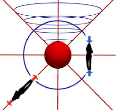
Figure 1: Tendex lines for a non-rotating (Schwarzschild) black hole. These lines are identical to those generated by a spherically symmetric mass distribution in the Newtonian limit. Also shown are observers who experience the tidal stretching and compression associated with the tendex lines.

V Slowly Rotating Black Hole

V.1 Slicing and coordinates

When the black hole is given a slow rotation with angular momentum per unit mass $a$, its metric (13) in Schwarzschild coordinates acquires an off-diagonal $g_{t\phi}$ term:

$$ds^{2} = -(1-{2M/r})dt^{2}+{dr^{2}\over 1-2M/r}+r^{2}d\theta^{2}$$ (19)

$$+r^{2}\sin^{2}\theta d\phi^{2}-{4aM\over r}\sin^{2}\theta dtd\phi\;$$

[the Kerr metric in Boyer-Lindquist coordinates, Eq. (VI.1) below, linearized in $a$]. The slices of constant EF time $\tilde{t}=t+2M\ln|r/2M-1|$ are still smoothly horizon penetrating, but the dragging of inertial frames (the off-diagonal $g_{t\phi}$ term in the metric) causes the Schwarzschild $\phi$ coordinate to become singular at the horizon. To fix this, we must “unwrap” $\phi$, e.g., by switching to

$$\tilde{\phi}=\phi+(a/2M)\ln|1-2M/r|\;,$$ (20)

thereby bringing the “slow-Kerr” metric (19) into the form

$$ds^{2} = -\biggl{(}1-\frac{2M}{r}\biggl{)}d\tilde{t}^{2}+\frac{4M}{r}d\tilde{t}dr+\biggl{(}1+\frac{2M}{r}\biggl{)}dr^{2}$$ (21)

$$+r^{2}d\theta^{2}+r^{2}\sin^{2}\theta d\tilde{\phi}^{2}-{4aM\over r}\sin^{2}\theta d\tilde{t}d\tilde{\phi}$$

$$-2a\sqrt{1+2M/r}\sin^{2}\theta drd\tilde{\phi}\;$$

[Eq. (B) below, linearized in $a$], which is well behaved at and through the horizon. The observers who move orthogonally to the slices of constant $\tilde{t}$ have 4-velocity $\vec{u}$ and orthonormal basis the same as for a non-rotating black hole, Eq. (16), except that $\vec{e}_{\hat{r}}$ is changed to

$$\vec{e}_{\hat{r}}={1\over\sqrt{1+2M/r}}\left[\partial_{r}+{a\over r^{2}}(1+2M/r)\partial_{\tilde{\phi}}\right]$$ (22)

[Eq. (46) below, linearized in $a$].

V.2 Frame-drag field and deformed tendex lines

The slow rotation gives rise to a frame-drag field

$$\mathcal{B}_{\tilde{r}\tilde{r}} = \frac{-6aM\cos\theta}{r^{4}}\;,\quad\mathcal{B}_{\tilde{r}\tilde{\theta}}=\mathcal{B}_{\tilde{\theta}\tilde{r}}=\frac{-3aM\sin\theta}{r^{4}\sqrt{1+2M/r}}\;,$$

$$\mathcal{B}_{\tilde{\theta}\tilde{\theta}} = \mathcal{B}_{\tilde{\phi}\tilde{\phi}}=\frac{3aM\cos\theta}{r^{4}}\;$$ (23)

[Eq. (40b) linearized in $a/M$] that lives in the slices of constant EF time $\tilde{t}$. This field’s vortex lines, shown in Fig. 2b, are poloidal and closely resemble those of a spinning point mass (a “current dipole”) in the linearized approximation to general relativity (Fig. 3 of Paper I Nichols et al. (2011)). At radii $r\gg M$, the field asymptotes to that of a linearized current dipole.

\begin{overpic}[width=195.12767pt]{SlowSpinKerrTendex_2} \put(5.0,10.0){\Large(a)} \end{overpic}

\begin{overpic}[width=195.12767pt]{SlowSpinKerrVortCone2} \put(5.0,10.0){\Large(b)} \end{overpic}

Figure 2: (a) Tendex lines, and (b) vortex lines for a slowly rotating (Kerr) black hole. Here we take $a/M=0.1$. The horizon is color coded by its tendicity $\mathcal{E}_{NN}$ in (a) (uniformly red signifying negative tendicity) and vorticity $\mathcal{B}_{NN}$ in (b), and the field lines are color coded by the sign of their tendicity or vorticity (blue for positive, red for negative). That is, the radial tendex lines, the vortex lines emerging from the north pole and the azimuthal vortex lines on the bottom carry negative tendicity or vorticity, while all other lines have positive tendicity or vorticity.) In (a), the spiraling lines have been made to spiral more loosely by multiplying the rate of change in the $r$ direction by five. The semi-transparent cone-like surfaces emerging from the horizon’s north and south polar regions show where the magnitude of the vorticity at a given radius has fallen to $80\%$ (outermost cones), $85\%$, and $90\%$ (innermost cones) of the polar magnitude. We identify the innermost cone (the 90% contour) as the edge of the frame-drag vortex. The equatorial plane is shown for reference in both panels.

The rotating hole’s horizon vorticity is $\mathcal{B}_{NN}=\mathcal{B}_{\hat{r}\hat{r}}=-6(aM/r^{4})\cos\theta$, which is negative in the north polar regions and positive in the south polar regions. Correspondingly, there is a counterclockwise frame-drag vortex sticking out of the hole’s north pole, and a clockwise one sticking out if its south pole. We identify the edge of each vortex, at radius $r$, as the location where the vorticities of the vortex lines that emerge from the hole at the base of the vortex, fall (as a function of $\theta$ at fixed $r$) to $90\%$ of the on-pole vorticity. The vortex edges are shown, in Fig. 2, as semi-transparent surfaces; for comparison we also show where the vorticity has fallen to $85\%$ and $80\%$ of the on-pole vorticity at a given radius $r$.

The hole’s (small) spin not only generates a frame-drag field $\mathcal{B}_{ij}$; it also modifies, slightly, the hole’s tidal field $\mathcal{E}_{ij}$ and its tendex lines. However, the spin does not modify the field’s tendicities, which (to first order in $a/M$) remain $\lambda_{r}^{\mathcal{E}}=-2M/r^{3}$, $\lambda_{\theta}^{\mathcal{E}}=\lambda_{\phi}^{\mathcal{E}}=M/r^{3}$ [Eq. (18)]. The modified unit tangent vectors to the tendex lines are

$$\vec{V}^{\mathcal{E}}_{r} = \vec{e}_{\hat{r}}-{2Ma\sin\theta\over r^{2}\sqrt{1+2M/r}}\vec{e}_{\hat{\tilde{\phi}}}\;,$$

$$\vec{V}^{\mathcal{E}}_{\tilde{\phi}} = \vec{e}_{\hat{\tilde{\phi}}}+{2Ma\sin\theta\over r^{2}\sqrt{1+2M/r}}\vec{e}_{\hat{r}}\;,\quad\vec{V}^{\mathcal{E}}_{\tilde{\theta}}=\vec{e}_{\hat{\tilde{\theta}}}\;.$$ (24)

Correspondingly, there is a slight (though hardly noticeable) bending of the radial tendex lines near the black hole, and—more importantly—the azimuthal tendex lines (the ones tangent to $\vec{V}^{\mathcal{E}}_{\tilde{\phi}}$) cease to close. Instead, the azimuthal tendex lines spiral outward along cones of fixed $\theta$, as shown in Fig. 2a. Since these lines have been only slightly perturbed from closed loops, they spiral quite tightly, appearing as solid cones. In order to better visualize these spiraling lines, we have increased their outward ($r$ directed) rate of change by a factor of five as compared to the axial rate of change in Fig. 2a.

V.3 Robustness of frame-drag field and tendex-line spiral

The two new features induced by the hole’s small spin (the frame-drag field, and the spiraling of the azimuthal tendex lines) are, in fact, robust under changes of slicing. We elucidate the robustness of the tendex spiral in Appendix C. We here elucidate the robustness of the frame-drag field and its vortex lines and vorticities:

Suppose that we change the time function $\tilde{t}$, which defines our time slices, by a small fractional amount of order $a/M$; i.e., we introduce a new time function

$$t^{\prime}=\tilde{t}+\xi(r,\theta)\;,$$ (25)

where $\tilde{t}$ is EF time and $\xi$ has been chosen axisymmetric and time-independent, so it respects the symmetries of the black hole’s spacetime. Then “primed” observers who move orthogonal to slices of constant $t^{\prime}$ will be seen by the EF observers (who move orthogonal to slices of constant $\tilde{t}$) to have small 3-velocities that are poloidal, ${\bf v}=v^{\hat{r}}{\bf e}_{\hat{r}}+v^{\hat{\theta}}{\bf e}_{\hat{\theta}}$. The Lorentz transformation from the EF reference frame to the primed reference frame at some event in spacetime induces a change of the frame-drag field given by

$$\delta\bm{\mathcal{B}}=-2({\bf v}\times\bm{\mathcal{E}})^{S}\;$$ (26)

[see, e.g., Eq. (B12) of Maartens (1998), linearized in small ${\bf v}$], where the $S$ means symmetrize. Inserting the EF tidal field (17) and the poloidal components of $\bf v$, we obtain as the only nonzero components of $\delta{\mathcal{B}}$

$$\delta\mathcal{B}_{\hat{r}\hat{\tilde{\phi}}}=\delta\mathcal{B}_{\hat{\tilde{\phi}}\hat{r}}=-(3M/r^{3})v^{\hat{\theta}}\;.$$ (27)

This axisymmetric, slicing-induced change of the frame-drag field does not alter the nonzero components of the frame-drag field in Eq. (23); it only introduces a change in the component $\mathcal{B}_{\hat{r}\hat{\tilde{\phi}}}$. This is a sense in which we mean the frame-drag field is robust. A simple calculation can show that one vorticity is unchanged, $\mathcal{B}_{\hat{\phi}\hat{\phi}}=3aM\cos\theta/r^{4}$, but the corresponding vortex line will no longer be a circle of constant $(r,\theta)$. Instead, it will wind on a sphere of constant $r$ relative to these closed azimuthal circles with an angle whose tangent is given by $v^{\hat{\theta}}\csc\theta\sqrt{r^{2}+2Mr}$. The poloidal vortex lines must twist azimuthally to remain orthogonal to these spiralling azimuthal lines, as well.

Although we will not see this specific kind of spiraling vortex lines in the next section on rapidly rotating Kerr black holes, we will see a different spiraling of the azimuthal vortex lines: spiraling on cones of constant $\theta$. We describe the reason for this in Appendix C.

VI Rapidly Rotating (Kerr) Black Hole

We shall now explore a rapidly rotating black hole described by the precise Kerr metric.

VI.1 Kerr metric in Boyer-Lindquist coordinates

The Kerr metric is usually written in Boyer-Lindquist (BL) coordinates $\{t,r,\theta,\phi\}$, where it takes the form

$$ds^{2} = -\left(1-\frac{2Mr}{\Sigma}\right)dt^{2}+\frac{\Sigma}{\Delta}dr^{2}+\Sigma d\theta^{2}+\frac{\sin^{2}\theta}{\Sigma}Ad\phi^{2}$$

$$-\frac{4Mar\sin^{2}\theta}{\Sigma}dtd\phi\,,$$

$$\Sigma = r^{2}+a^{2}\cos^{2}\theta\,,$$

$$\Delta = r^{2}-2Mr+a^{2}\,,$$

$$A = (r^{2}+a^{2})^{2}-a^{2}\Delta\sin^{2}\theta\,,$$ (28)

Because the slices of constant $t$ are singular at the horizon (and therefore not of much interest to us), we relegate to Appendix A the details of their tidal and frame-drag fields, and their vortex and tendex lines.

VI.2 Horizon-penetrating slices

In our study of Kerr black holes, we shall employ two different slicings that penetrate the horizon smoothly: surfaces of constant Kerr-Schild time coordinate $\tilde{t}$, and surfaces of constant Cook-Scheel time coordinate $\bar{t}$. By comparing these two slicings’ tendex lines with each other, and also their vortex lines with each other, we shall gain insight into the lines’ slicing dependence.

The Kerr-Schild (Kerr (1963); Boyer and Lindquist (1967), see also, e.g., Exercise 33.8 of Misner et al. (1973)) time coordinate (also sometimes called ingoing-Kerr time) is defined by

$$\tilde{t}=t+r_{*}-r\;,\quad\hbox{where }\frac{dr_{*}}{dr}=\frac{r^{2}+a^{2}}{\Delta}\;.$$ (29)

The Cook-Scheel Cook and Scheel (1997) time coordinate is

$$\bar{t} =t+\frac{r_{+}^{2}+a^{2}}{r_{+}-r_{-}}\text{ln}\left|\frac{r-r_{+}}{r-r_{-}}\right|\;$$

$$=\tilde{t}+2M\text{ln}\left|\frac{2M}{r-r_{-}}\right|\;,$$ (30)

(see Eqs. (19) and (20) of Cook and Scheel (1997)) where $r_{+}$ is the value of the Boyer-Lindquist radial coordinate $r$ at the event horizon, and $r_{-}$ is its value at the (inner) Cauchy horizon:

$$r_{\pm}=M\pm\sqrt{M^{2}-a^{2}}\;.$$ (31)

Figure 3: Slices of constant Boyer-Lindquist time $t$, Kerr-Schild time $\tilde{t}$, and Cook-Scheel time $\bar{t}$, drawn in a Kerr-Schild spacetime diagram for a black hole with $a/M=0.95$.

Figure 3 shows the relationship between these slicings for a black hole with $a/M=0.95$. In this figure, horizontal lines are surfaces of constant Kerr-Schild time $\tilde{t}$. Since $t$, $\bar{t}$ and $\tilde{t}$ differ solely by functions of $r$, the surfaces of constant Cook-Scheel time $\bar{t}$ are all parallel to the $\bar{t}=0$ surface shown in the figure, and the surfaces of constant Boyer-Lindquist time $t$ are all parallel to the $t=0$ surface. The Kerr-Schild and Cook-Scheel surfaces penetrate the horizon smoothly. By contrast, the Boyer-Lindquist surfaces all asymptote to the horizon in the deep physical past, never crossing it; i.e., they become physically singular at the horizon.

VI.3 Horizon-penetrating coordinate systems

Not only is the Boyer-Lindquist time coordinate $t$ singular at the event horizon; so is the Boyer-Lindquist azimuthal angular coordinate $\phi$. It winds around an infinite number of times as it asymptotes to the horizon. We shall use two different ways to unwind it, associated with two different horizon-penetrating angular coordinates: The ingoing-Kerr coordinate

$$\tilde{\phi}=\phi+\frac{a}{r_{+}-r_{-}}\text{ln}\left|\frac{r-r_{+}}{r-r_{-}}\right|=\phi+\int_{r}^{\infty}{a\over\Delta}dr\;,$$ (32)

and the Kerr-Schild coordinate

$$\varphi=\tilde{\phi}-\tan^{-1}(a/r)\;.$$ (33)

Figure 4: Curves of constant Boyer-Lindquist angle $\phi$, Kerr-Schild angle $\varphi$, and ingoing-Kerr angle $\tilde{\phi}$ for a black hole with $a/M=0.95$.

Figure 4 shows the relationship of these angular coordinates for a black hole with $a/m=0.95$. Notice that: (i) all three angular coordinates become asymptotically the same as $r\rightarrow\infty$; (ii) the two horizon-penetrating coordinates, ingoing-Kerr $\tilde{\phi}$ and Kerr-Schild $\varphi$, differ by less than a radian as one moves inward to the horizon; and (iii) the Boyer-Lindquist coordinate $\phi$ plunges to $-\infty$ (relative to horizon-penetrating coordinates) as one approaches the horizon, which means it wraps around the horizon an infinite number of times.

In the literature on Kerr black holes, four sets of spacetime coordinates are often used:

• Boyer-Lindquist coordinates, $\{t,r,\theta,\phi\}$ . These are the coordinates in Sec. VI.1.

• Ingoing-Kerr coordinates, $\{\tilde{t},r,\theta,\tilde{\phi}\}$. Often in this case $\tilde{t}$ is replaced by a null coordinate, $v=\tilde{t}+r$ (curves $v=$ const, $\theta=$ const, and $\tilde{\phi}=$ const are ingoing null geodesics).

• Quasi-Cartesian Kerr-Schild coordinates, $\{\tilde{t},x,y,z\}$ and their cylindrical variant $\{\tilde{t},\varpi,z,\varphi\}$. Here

  $$x+iy = (r+ia)e^{i\tilde{\phi}}\sin\theta\;,\quad z=r\cos\theta\;,$$

  $$\varpi = \sqrt{x^{2}+y^{2}}=\sqrt{r^{2}+a^{2}}\sin^{2}\theta\;,$$

  $$\varphi = \arctan(y/x)=\tilde{\phi}+\arctan(a/r)\;.$$ (34)

  The Kerr-Schild spatial coordinates $\{x,y,z\}$ resemble the coordinates typically used in numerical simulations of binary black holes at late times, when the merged hole is settling down into its final, Kerr state. These coordinate systems resemble each other in the senses that (i) both are quasi-Cartesian, and (ii) for a fast-spinning hole, the event horizon in both cases, when plotted in the coordinates being used, looks moderately oblate. For this reason, in our study of Kerr black holes, we shall focus our greatest attention on Kerr-Schild coordinates. The Kerr metric, written in Kerr-Schild coordinates, has the form

  $$ds^{2} = \left(\eta_{\mu\nu}+\frac{2Mr^{3}}{r^{4}+a^{2}z^{2}}k_{\mu}k_{\nu}\right)dx^{\mu}dx^{\nu}\,,$$

  $$k_{\mu} = \left(1,\frac{rx+ay}{r^{2}+a^{2}},\frac{ry-ax}{r^{2}+a^{2}},\frac{z}{r}\right)\,,$$ (35)

  where $r$ is the Boyer-Lindquist radial coordinate, and is the larger root of

  $$x^{2}+y^{2}+z^{2}=r^{2}+a^{2}\left(1-\frac{z^{2}}{r^{2}}\right)\,,$$ (36)

  and $\eta_{\mu\nu}$ is the usual flat Minkowski metric.

• Cook-Scheel harmonic coordinates Cook and Scheel (1997), $\{\bar{t},\bar{x},\bar{y},\bar{z}\}$ where $\bar{t}$ is given by Eq. (30), while the spatial coordinates are defined by

  $$\bar{x}+i\bar{y} = \left[r-M+ia\right]e^{i\tilde{\phi}}\sin(\theta)$$ (37)

  $$\bar{z} = \left[r-M\right]\cos(\theta)$$ (38)

  These coordinates are harmonic in the sense that the scalar wave operator acting on them vanishes. In these coordinates, the event horizon of a spinning black hole is more oblate than in Kerr-Schild coordinates—and much more oblate for $a/M$ near unity.

VI.4 Computation of tendex and vortex lines, and their tendicities and vorticities

Below we show pictures of tendex and vortex lines, color coded with their tendicities and vorticities, for our two horizon-penetrating slicings and using our three different sets of spatial coordinates. In all cases we have computed the field lines and their eigenvalues numerically, beginning with analytical formulas for the metric. More specifically, after populating a numerical grid using analytical expressions for the metric, we numerically compute $\mathcal{E}_{ij}$ and $\mathcal{B}_{ij}$, as well as their eigenvalues and eigenvectors. A numerical integrator is then utilized to generate the tendex and vortex lines. Finally, we apply analytical transformations that take these lines to whatever spatial coordinate system we desire.

Although not required for the purpose of generating the figures in the following sections, it is nevertheless possible to find analytical expressions for $\mathcal{E}_{ij}$ and $\mathcal{B}_{ij}$, and subsequently their eigenvalues and eigenvectors. These expressions provide valuable insights into the behavior of the tendex and vortex lines, and we present such results for the ingoing-Kerr coordinates in Appendix B.

VI.5 Kerr-Schild slicing: Tendex and vortex lines in several spatial coordinate systems

Once the slicing is chosen, the tidal and frame-drag fields, and also the tendex and vortex lines and their tendicities and vorticities, are all fixed as geometric, coordinate-independent entities that live in a slice. If we could draw an embedding diagram showing the three-dimensional slice isometrically embedded in a higher-dimensional flat space, then we could visualize the tendex and vortex lines without the aid of a coordinate system. However, the human mind cannot comprehend embedding diagrams in such high-dimensional spaces, so we are forced to draw the tendex and vortex lines in some coordinate system for the slice, in a manner that makes the coordinate system look like it is one for flat space.

Such a coordinate-diagram plot of the lines makes them look coordinate dependent—i.e., their shapes depend on the coordinate system used. Nevertheless, the lines themselves are geometrically well-defined, independent of coordinate system, and they map appropriately between them. The visual features of these lines are also qualitatively similar in reasonable coordinate systems.

Figure 5 is an important example. It shows the tendex lines (left column of plots) and vortex lines (right column of plots) for a fast-spinning Kerr black hole, with $a=0.95M$. We have also colored the horizon of the black hole according to its horizon tendicity and vorticity, respectively. In all cases the slicing is Kerr-Schild; i.e., the lines lie in a slice of constant $\tilde{t}$. The three rows of figures are drawn in three different spatial coordinate systems: ingoing-Kerr, Kerr-Schild, and Cook-Scheel.

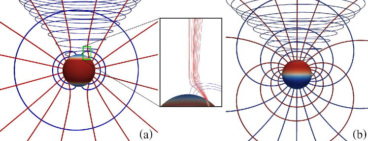
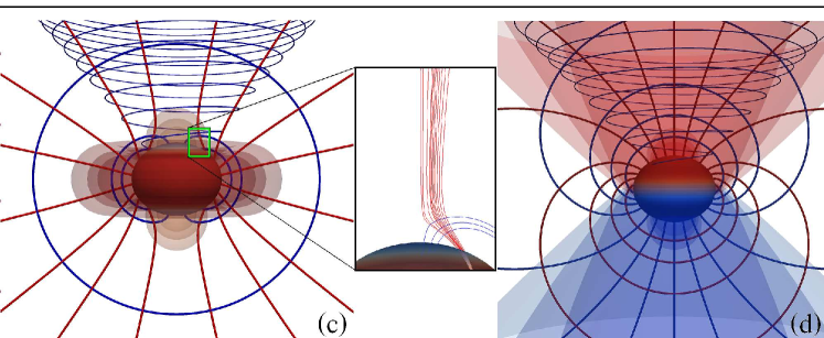
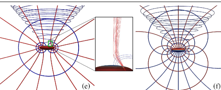
Figure 5: Kerr black hole with $a/M=0.95$ in Kerr-Schild slicing, drawn in three different spatial coordinate systems. The left and center columns of drawings [panels (a), (c), (e)] show tendex lines; the right column of drawings [panels (b), (d), (f)] show vortex lines. The three rows, from top downward, use ingoing-Kerr spatial coordinates $\{r,\theta,\tilde{\phi}\}$ [panels (a) and (b)], Kerr-Schild spatial coordinates $\{x,y,z\}$ [panels (c) and (d)], and Cook-Scheel spatial coordinates $\{\bar{x},\bar{y},\bar{z}\}$ [panels (e) and (f)]. In all cases, the lines with positive tendicity or vorticity are colored blue; those with negative tendicity or vorticity are colored red. (The radial tendex lines and vortex lines emerging from the top half of the horizon are red, while all other lines are blue.) The horizon is shown with its horizon tendicity (left column of drawings) and horizon vorticity (right column) color coded from dark blue for strongly positive to dark red for strongly negative. (Horizon tendicity is negative near the equator and positive near the poles. Vorticity on the other hand transitions from being negative on top to positive on the bottom.) In Kerr-Schild coordinates [panels (c) and (d)], we have also shown as semi-transparent surfaces, contours of $\tilde{r}^{3}$ times tendicity and $\tilde{r}^{4}$ times vorticity, where $\tilde{r}^{2}=x^{2}+y^{2}+z^{2}$ for Kerr-Schild spatial coordinates. In panel (c), the innermost equatorial contour has the most negative tendicity while the others have $90\%,80\%,30\%,20\%,$ and $10\%$ this value, and the innermost polar contour has the least negative tendicity. In panel (d) the contour with the most negative vorticity consists of the innermost red cone and the outermost red bubble (at the north pole), and the others are at $90\%$ and $80\%$ this value. The blue contours of panel (d) (at the bottom half of that panel) are arranged similarly but with positive vorticity.

Notice the following important features of this figure:

• As expected, the qualitative features of the tendex lines are independent of the spatial coordinates. The only noticeable differences from one coordinate system to another are a flattening of the strong-gravity region near the hole as one goes from ingoing-Kerr coordinates (upper row of panels) to Kerr-Schild coordinates (center row of panels) and then a further flattening for Cook-Scheel coordinates (bottom row of panels).

• The azimuthal (toroidal) tendex and vortex lines (those that point predominantly in the $\vec{e}_{\tilde{\phi}}$ direction) spiral outward from the horizon along cones of constant $\theta$, as for the tendex lines of a slowly spinning black hole [cf. the form of $\vec{V}_{\hat{\tilde{\phi}}}$ in Eqs. (50)]. As we shall discuss in Appendix C, this is a characteristic of a large class of commonly used, horizon-penetrating slicings of spinning black holes.

• All the poloidal tendex and vortex lines have (small) azimuthal ($\tilde{\phi}$) components, which do not show up in this figure; see the $\vec{e}_{\hat{\tilde{\phi}}}$ components of the eigenvectors $\vec{V}^{\mathcal{E}}_{r}$, $\vec{V}^{\mathcal{E}}_{\theta}$, $\vec{V}^{\mathcal{B}}_{-}$ and $\vec{V}^{\mathcal{B}}_{+}$ in Eqs. (50) and (51).

• Left column of drawings: For this rapidly spinning black hole, the horizon tendicity is positive (blue) in the north and south polar regions, and negative (red) in the equatorial region, by contrast with a slowly spinning hole, where the horizon tendicity is everywhere negative (Fig. 2). Correspondingly, a radially oriented person falling into a polar region of a fast-spinning hole gets squeezed from head to foot, rather than stretched, as conventional wisdom demands. The relationship $\mathcal{E}_{NN}=-\mathcal{R}/2$ between the horizon’s tendicity and its scalar curvature tells us that this peculiar polar feature results from the well-known fact that, when the spin exceeds $a/M=\sqrt{3}/2\approx 0.8660$, the scalar curvature goes negative near the poles, at angles $\theta$ satisfying $2(a/M)^{2}\cos^{2}\theta>1+\sqrt{1-(a/M)^{2}}$. This negative scalar curvature is also responsible for the fact that is it impossible to embed the horizon’s 2-geometry in a 3-dimensional Euclidean space when the spin exceeds $a/M=\sqrt{3}/2$ Smarr (1973).

• Left column of drawings: The blue (positive tendicity) tendex lines that emerge from the north polar region sweep around the hole, just above the horizon, and descend into the south polar region. In order to stay orthogonal to these blue (squeezing) tendex lines, the red (stretching) lines descending from radial infinity get deflected away from the horizon’s polar region until they reach a location with negative tendicity (positive scalar curvature), where they can attach to the horizon; see the central panels, which are enlargements of the north polar region for the left panels.

• Right column of drawings: The vortex-line structure for this fast-spinning black hole is very similar to that for the slow-spinning hole of Fig. 2, and similar to that for a spinning point mass in the linear approximation to general relativity (Fig. 3 of Paper I Nichols et al. (2011)). The principal obvious change is that the azimuthal vortex lines are not closed; instead, they spiral away from the black hole, like the azimuthal tendex lines.

• Right column of drawings: Most importantly, as for a slow-spinning black hole, there are two vortexes (regions of strong vorticity): as a counterclockwise vortex emerging from the north polar region, and a clockwise vortex emerging from the south polar region. As we shall see in Paper IV, when two spinning black holes collide and merge, these vortexes sweep around, emitting gravitational waves. In Fig. 5(d), these vortexes are indicated by contours of $\tilde{r}^{4}$ times vorticity, where $\tilde{r}^{2}=x^{2}+y^{2}+z^{2}$ for Kerr-Schild coordinates $\{x,y,z\}$. Notice in particular that each contour consists of one cone together with one bubble attached to the horizon, with the bubbles enclosing the polar regions excluding them from the vortexes. This is a feature not seen for the slow-spinning case.

VI.6 Slicing-dependence of tendex and vortex lines

To explore how a Kerr black hole’s vortex and tendex lines depend on the choice of slicing, we focus in Fig. 6 on a black hole with $a/M=0.875$, viewed in a slice of constant Kerr-Schild time, $\tilde{t}=$constant, and in a slice of constant Cook-Scheel harmonic time, $\bar{t}=$constant. In the two slices, we use the same spatial coordinates: Kerr-Schild. (We chose $a/M=0.875$, rather than the $0.95$ that we used for exploring spatial coordinate dependence, because it is simpler to handle numerically in the Cook-Scheel slicing.)

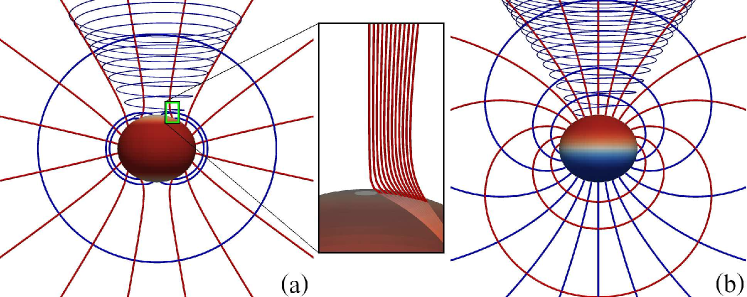
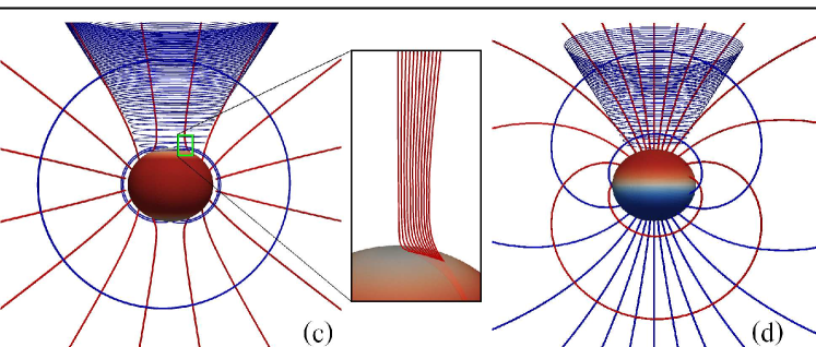
Figure 6: Tendex lines and vortex lines for a Kerr black hole with $a/M=0.875$ in Kerr-Schild spatial coordinates, for two different slicings: Kerr-Schild $\tilde{t}=$constant, and Cook-Scheel $\bar{t}=$constant. The left and center columns of drawings [panels (a) and (c)] show tendex lines; the right column of drawings [panels (b) and (d)] show vortex lines. The top row of drawings [panels (a) and (b)] is for Kerr-Schild slicing; the bottom row [panels (c) and (d)] is for Cook-Scheel slicing. Since the slicings are different, it is not possible to focus on the same sets of field lines in the Kerr-Schild (upper panels) and Cook-Scheel (lower panels) cases. However, we have attempted to identify similar field lines by ensuring they pass through the same Kerr-Schild spatial coordinate locations on selected surfaces. (The color of the lines and horizon are similar to Fig. 5)

The most striking aspect of Fig. 6 is the close similarity of the tendex lines (left column of drawings) in the two slicings (upper and lower drawings), and also the close similarity of the vortex lines (right column of drawings) in the two slicings (upper and lower). There appears to be very little slicing dependence when we restrict ourselves to horizon-penetrating slicings.

By contrast, if we switch from a horizon-penetrating to a horizon-avoiding slice, there are noticeable changes in the field lines: Compare the top row of Fig. 6 ($a/M=0.875$ for a Kerr-Schild, horizon-penetrating slice) with Fig. 7 (the same hole, $a/M=0.875$, for a Boyer-Lindquist, horizon-avoiding slice), concentrating for now on panels (a) and (b) depicting tendex and vortex lines in Boyer-Lindquist spatial coordinates. The most striking differences are (i) the radial tendex lines’ failure to reach the horizon for horizon-avoiding slices, contrasted with their plunging through the horizon for horizon-penetrating slices, and (ii) the closed azimuthal tendex and vortex lines for Boyer-Lindquist horizon-avoiding slices, contrasted with the outward spiraling azimuthal lines for horizon-penetrating slices. In Appendix C we show that this outward spiral is common to a class of horizon-penetrating slices. Lastly, we note that Fig. 7 (a) and (b) are plotted using Boyer-Lindquist spatial coordinates in order to compare with analytical expressions given in that appendix. When we use Kerr-Schild spatial coordinates, as is done in Fig. 6, in order to facilitate a more appropriate comparison, we observe that the Boyer-Lindquist azimuthal coordinate singularity depicted in Fig. 4 causes the tendex and vortex lines in Boyer-Lindquist slicing to wind in $\phi$ direction when close to horizon. This feature is clearly visible in Fig. 7 (c) and (d), where we display the tendex and vortex lines in Kerr-Schild spatial coordinates.

Based on our comparison of Kerr-Schild and Cook-Scheel slicings (Fig. 6), and our analysis of the ubiquity of azimuthal spiraling lines in horizon-penetrating slices (Appendix C), we conjecture that horizon-penetrating slicings of any black-hole spacetime will generically share the same qualitative and semi-quantitative structures of tendex and vortex lines. This conjecture is of key importance for our use of tendex and vortex lines to extract intuition into the dynamical processes observed in numerical simulations. More specifically:

Numerical spacetimes have dynamically chosen slicings, and the primary commonality from simulation to simulation is that the time slicing must be horizon penetrating, to prevent coordinate singularities from arising on the numerical grid near the horizon. Our conjecture implies that, regardless of the precise slicing used in a simulation, we expect the tendex and vortex lines to faithfully reveal the underlying physical processes. We will build more support for this conjecture in Paper III, by comparing the final stages of a numerical black-hole merger with a perturbed Kerr black hole, using very different slicing prescriptions.

We conclude this section with a digression from its slicing-dependence focus:

When we compare the $a/M=0.875$ black hole of Fig. 6 with the $a/M=0.95$ hole of Fig. 5, the most striking difference is in the tendex lines very near the horizon. The value $a/M=0.875$ is only slightly above the critical spin $a/M=\sqrt{3}/2=0.8660$ at which the horizon’s poles acquire negative scalar curvature. Correspondingly, for $a/M=0.875$, the blue tendex lines that connect the two poles emerge from a smaller region at the poles than for $a/M=0.95$, and they hug the horizon more tightly as they travel from one pole to the other; and the red, radial tendex lines near the poles suffer much smaller deflections than for $a/M=0.95$ as they descend into the horizon (see insets).

VII Conclusion

Using vortex and tendex lines and their vorticities and tendicities, we have visualized the spacetime curvature of stationary black holes. Stationary black-hole spacetimes are a simple arena in which to learn about the properties of these visualization tools in regions of strong spacetime curvature. From the features of the vortex and tendex lines and their vorticities and tendicities that we describe below, we have gained an understanding of these visualization tools and made an important stride toward our larger goal of using these tools to identify geometrodynamical properties of strongly curved spacetimes—particularly those in the merger of binary black holes.

Black hole spacetimes have an event horizon (a feature that was absent in our study of weakly gravitating systems in Paper I). To understand our visualization tools on the horizon, we defined and discussed the horizon tendicity and horizon vorticity of stationary black holes. The horizon tendicity and vorticity are directly proportional to the intrinsic and extrinsic curvature scalars of a two-dimensional horizon. As a result, the average value of the horizon tendicity must be negative, and the horizon vorticity must average to zero. Any region of large vorticity on the horizon (a horizon vortex), therefore, must be accompanied by an equivalent vortex of the opposite sign, but there is not an analogous constraint for horizon tendexes.

Outside the horizon, we also visualized the tendex lines and vortex lines, the tendicities and vorticities, and the regions of large tendicity (tendexes) and large vorticity (vortexes) for Schwarzschild and Kerr black holes (the latter both slowly and rapidly spinning). In particular, we investigated how the vortex and tendex lines of Kerr black holes changed when they were drawn in different time slices and with different spatial coordinates—within the set of those time slices that smoothly pass through the horizon and spatial coordinates that are everywhere regular. We found our visualizations are quite similar between two commonly used, though rather different, horizon-penetrating time functions: Kerr-Schild and Cook-Scheel. The spatial-coordinate dependence was also mild, and was easily understandable in terms of the relation between the different coordinate systems. Because the coordinate systems used in numerical simulations of black holes are also horizon penetrating, this suggests that the vortex and tendex lines will not be very different, even though the dynamical coordinates of the simulation may be.

This study is a foundation for future work on computing the tendexes and vortexes of black-hole spacetimes. A recent work by Dennison and Baumgarte Dennison and Baumgarte (2012a)—in which the authors calculated the tendex and vortex fields of approximate initial data representing non-spinning, boosted black holes, and also black-hole binaries—will also be helpful for understanding binaries. In addition, our investigations of the slicing and coordinate dependence of tendexes and vortexes is complemented by another recent study of Dennison and Baumgarte Dennison and Baumgarte (2012b), where expressions are given for computing curvature invariants in terms of the vorticities, tendicities, and the eigenvector fields which give the tendex and vortex lines. These expressions will likely be of use in future analytic and numerical studies of tendexes and vortexes.

In a companion paper (Paper III), we turn to perturbed black holes. We aim to deepen our understanding of tendex and vortex lines in these well-understood situations and to see what new insights we can draw from these spacetimes by using vortex and tendex lines. Ultimately, we will apply these visualization techniques and our intuition from simpler analytical spacetimes to study numerical simulations of strongly curved and dynamic spacetimes and their geometrodynamics. In Paper IV, we will do just this, focusing on binary-black-hole mergers.

Appendix A Kerr Black Hole in Boyer-Lindquist Slicing and Coordinates

For a rapidly rotating Kerr black hole in Boyer-Lindquist (BL) coordinates $\{t,r,\theta,\phi\}$, the metric is given by Eq. (VI.1) above. A “BL observer”, who moves orthogonally to the slices of constant BL time $t$, has a 4-velocity $\vec{u}$ and orthonormal tetrad given by

$$\vec{u} =\sqrt{\frac{A}{\Sigma\Delta}}\left(\partial_{t}-\frac{2Mar}{A}\partial_{\phi}\right)\,, \vec{e}_{\hat{r}} =\sqrt{\frac{\Delta}{\Sigma}}\partial_{r}\,,$$

$$\vec{e}_{\hat{\theta}} =\frac{1}{\sqrt{\Sigma}}\partial_{\theta}\,, \vec{e}_{\hat{\phi}} =\sqrt{\frac{\Sigma}{A}}\frac{1}{\sin\theta}\partial_{\phi}\,.$$ (39)

This tetrad is also often called the locally nonrotating frame Bardeen (1970); Bardeen et al. (1972). In this orthonormal basis, the tidal and frame-drag fields are given by (cf. Eqs. (6.8a-6.9d) of Thorne et al. (1986))

$$\mathcal{E}_{\hat{a}\hat{b}} = \begin{pmatrix}-Q_{e}\frac{2+\xi}{1-\xi}&\mu Q_{m}&0\\ *&Q_{e}\frac{1+2\xi}{1-\xi}&0\\ *&*&Q_{e}\end{pmatrix}\,,$$ (40a)

$$\mathcal{B}_{\hat{a}\hat{b}} = \begin{pmatrix}-Q_{m}\frac{2+\xi}{1-\xi}&-\mu Q_{e}&0\\ *&Q_{m}\frac{1+2\xi}{1-\xi}&0\\ *&*&Q_{m}\end{pmatrix}\,,$$ (40b)

with entries denoted by $$*$$ fixed by the symmetry of the tensors, and where

$$Q_{e}=\frac{Mr(r^{2}-3a^{2}\cos^{2}\theta)}{\Sigma^{3}}\,,$$ (40c)

$$Q_{m}=\frac{Ma\cos\theta(3r^{2}-a^{2}\cos^{2}\theta)}{\Sigma^{3}}\,,$$ (40d)

$$\xi=\frac{\Delta a^{2}\sin^{2}\theta}{(r^{2}+a^{2})^{2}}\,,$$ (40e)

$$\mu=\frac{3a\sqrt{\Delta}(r^{2}+a^{2})\sin\theta}{A}=\frac{3\sqrt{\xi}}{1-\xi}\,.$$ (40f)

The functions $Q_{e}$ and $Q_{m}$ are related to the real and imaginary parts of the complex Weyl scalar $\Psi_{2}$ calculated using the Kinnersley null tetrad by $\Psi_{2}=-Q_{e}+iQ_{m}$. Note that there is a duality between the electric and the magnetic curvature tensors: namely, by replacing $Q_{e}\to Q_{m}$ and $Q_{m}\to-Q_{e}$, the tensor transforms as $\mathcal{E}_{\hat{a}\hat{b}}\to\mathcal{B}_{\hat{a}\hat{b}}$.

The block diagonal forms of $\mathcal{E}_{\hat{a}\hat{b}}$ and $\mathcal{B}_{\hat{a}\hat{b}}$ imply that one of the eigenvectors for each will be $\vec{e}_{\phi}$. When integrated, this gives toroidal tendex and vortex lines (i.e., lines that are azimuthal, closed circles). The other two sets of lines for each tensor are poloidal (i.e., they lie in slices of constant $\phi$).

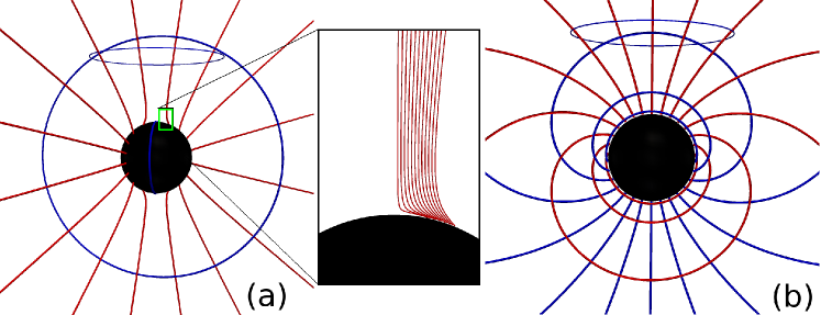
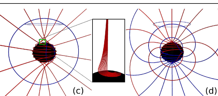
Figure 7: (a) Tendex lines for a Kerr black hole with $a/M=0.875$ on a slice of constant Boyer-Lindquist time $t$, plotted in Boyer-Lindquist spatial coordinates. The lines with positive tendicity are colored blue and negative are colored red. (b) Vortex lines for this same black hole, slicing and coordinates, with lines of positive vorticity colored blue and negative colored red. (c) and (d) Tendex and vortex lines for the same black hole and same Boyer-Lindquist slicing, but drawn in the Kerr-Schild spatial coordinates. (The color of the lines and horizon are similar to Fig. 5)

More specifically, the eigenvectors of the tidal field are

$$\vec{V}^{\mathcal{E}}_{r} = {(\lambda_{r}^{\mathcal{E}}-\mathcal{E}_{\hat{\theta}\hat{\theta}})\vec{e}_{\hat{r}}+\mathcal{E}_{\hat{r}\hat{\theta}}\vec{e}_{\hat{\theta}}\over\sqrt{(\lambda_{r}^{\mathcal{E}}-\mathcal{E}_{\hat{\theta}\hat{\theta}})^{2}+(\mathcal{E}_{\hat{r}\hat{\theta}})^{2}}}\,,$$

$$\vec{V}^{\mathcal{E}}_{\theta} = {(\lambda_{\theta}^{\mathcal{E}}-\mathcal{E}_{\hat{\theta}\hat{\theta}})\vec{e}_{\hat{r}}+\mathcal{E}_{\hat{r}\hat{\theta}}\vec{e}_{\hat{\theta}}\over\sqrt{(\lambda_{\theta}^{\mathcal{E}}-\mathcal{E}_{\hat{\theta}\hat{\theta}})^{2}+(\mathcal{E}_{\hat{r}\hat{\theta}})^{2}}}\,,$$

$$\vec{V}^{\mathcal{E}}_{\phi} = \vec{e}_{\hat{\phi}}\,.$$ (41)

The labeling of these eigenvectors is such that, as $a\rightarrow 0$, they limit to the corresponding eigenvectors (18) of a Schwarzschild black hole. The tendicities (eigenvalues) associated with these three eigenvectors, which appear in the above formulas, are

$$\lambda_{r}^{\mathcal{E}} = -\frac{Q_{e}}{2}-\sqrt{\left(\frac{3Q_{e}}{2}\right)^{2}\biggl{(}\frac{1+\xi}{1-\xi}\biggr{)}^{2}+\mu^{2}Q_{m}^{2}}\,,$$

$$\lambda_{\theta}^{\mathcal{E}} = -\frac{Q_{e}}{2}+\sqrt{\left(\frac{3Q_{e}}{2}\right)^{2}\biggl{(}\frac{1+\xi}{1-\xi}\biggr{)}^{2}+\mu^{2}Q_{m}^{2}}\,,$$

$$\lambda_{\phi}^{\mathcal{E}} = Q_{e}\,,$$ (42)

The eigenvectors of the frame-drag field are

$$\vec{V}^{\mathcal{B}}_{\pm} = {(\lambda^{\mathcal{B}}_{\pm}-\mathcal{B}_{\hat{\theta}\hat{\theta}})\vec{e}_{\hat{r}}+\mathcal{B}_{\hat{r}\hat{\theta}}\vec{e}_{\hat{\theta}}\over\sqrt{(\lambda^{\mathcal{B}}_{\pm}-\mathcal{B}_{\hat{\theta}\hat{\theta}})^{2}+(\mathcal{B}_{\hat{r}\hat{\theta}})^{2}}}\,,$$

$$\vec{V}^{\mathcal{B}}_{\phi} = \vec{e}_{\hat{\phi}}\,.$$ (43)

Here the labeling $+$ and $-$ of the poloidal eigenvectors corresponds to the signs of their eigenvalues (vorticities). The eigenvalues are

$$\lambda_{\pm}^{\mathcal{B}} = -\frac{Q_{m}}{2}\pm\sqrt{\left(\frac{3Q_{m}}{2}\right)^{2}\biggl{(}\frac{1+\xi}{1-\xi}\biggr{)}^{2}+\mu^{2}Q_{e}^{2}}\,,$$

$$\lambda_{\phi}^{\mathcal{B}} = Q_{m}\,.$$ (44)

The tendex and vortex lines tangent to the eigenvectors (41) and (43) are shown in Fig. 7 for a rapidly rotating black hole, $a/M=0.875$. The lines with positive eigenvalues (tendicity or vorticity) are colored blue, and those with negative eigenvalues are colored red. Far from the black hole, the tendex lines resemble those of a Schwarzschild black hole, and the vortex lines resemble those of a slowly spinning hole. However, near the horizon the behavior is quite different. The nearly radial tendex lines in the inset of Fig. 7 are bent sharply as they near the horizon, because of the black hole’s spin.

Before closing this appendix, we describe the behavior of the eigenvalues near the poles. From Eqs. (42), we see that as $\theta\to 0$ and $\theta\to\pi$, $\lambda^{\mathcal{E}}_{\theta}\to\lambda^{\mathcal{E}}_{\phi}$. Along the polar axis, therefore, the poloidal and axial eigenvectors of $\mathcal{E}_{\hat{a}\hat{b}}$ become degenerate, and any vector in the plane spanned by these directions is also an eigenvector at the axis. Meanwhile, for $\mathcal{B}_{\hat{a}\hat{b}}$, Eqs. (44) show that as $\theta\to 0$, $\lambda^{\mathcal{B}}_{+}\to\lambda^{\mathcal{B}}_{\phi}$, and as $\theta\to\pi$, $\lambda^{\mathcal{B}}_{-}\to\lambda^{\mathcal{B}}_{\phi}$. Once again there is a degenerate plane spanned by two eigenvectors at the polar axis. In Paper III, in which we study the tendex and vortex lines of perturbed Kerr black holes, the degenerate regions have a strong influence on the perturbed tendex and vortex lines (see Appendix F of Paper III).

Appendix B Kerr Black Hole in Kerr-Schild Slicing and Ingoing-Kerr Coordinates

In ingoing-Kerr coordinates $\{\tilde{t},r,\theta,\tilde{\phi}\}$ [Eqs. (29) and (32)], the Kerr metric takes the form (see, e.g., Chapter 33 of Misner et al. (1973), though we use the Kerr-Schild time $\tilde{t}$ Kerr (1963); Boyer and Lindquist (1967), or Eq. (D.4) of Gourgoulhon and Jaramillo (2006))

$$ds^{2} = -\biggl{(}1-\frac{2Mr}{\Sigma}\biggr{)}d\tilde{t}^{2}+\frac{4Mr}{\Sigma}drd\tilde{t}-\frac{4Mar\sin^{2}\theta}{\Sigma}d\tilde{t}d\tilde{\phi}$$

$$+H^{2}dr^{2}+\Sigma d\theta^{2}-2aH\sin^{2}\theta drd\tilde{\phi}+\frac{A\sin^{2}\theta}{\Sigma}d\tilde{\phi}^{2}\,,$$

$$H^{2} = 1+\frac{2Mr}{\Sigma}\,,$$ (45)

where $\Sigma$ and $A$ are defined in Eq. (VI.1). The 4-velocities of ingoing-Kerr observers, who move orthogonally to slices of constant $\tilde{t}$, and the orthonormal tetrads they carry, are given by

$$\vec{u} =H\partial_{\tilde{t}}-\frac{2Mr}{H\Sigma}\partial_{r}\,, \vec{e}_{\hat{r}} =\frac{\sqrt{A}}{H\Sigma}\partial_{r}+\frac{aH}{\sqrt{A}}\partial_{\tilde{\phi}}\,,$$

$$\vec{e}_{\hat{\theta}} =\frac{1}{\sqrt{\Sigma}}\partial_{\theta}\,, \vec{e}_{\hat{\tilde{\phi}}} =\sqrt{\frac{\Sigma}{A}}\frac{1}{\sin\theta}\partial_{\tilde{\phi}}\,$$ (46)

(see, e.g., King et al. (1975) or Gourgoulhon and Jaramillo (2006)).

The components of the tidal field in this orthonormal basis are

$$\mathcal{E}_{\hat{a}\hat{b}}=\begin{pmatrix}-Q_{e}\frac{2+\xi}{1-\xi}&Q_{m}\frac{3a(r^{2}+a^{2})\sin\theta}{H\sqrt{A\Sigma}}&Q_{e}\frac{6aMr(r^{2}+a^{2})\sin\theta}{HA\sqrt{\Sigma}}\\ *&Q_{e}\left(1+\frac{3a^{2}\sin^{2}\theta}{H^{2}\Sigma}\right)&-Q_{m}\frac{6a^{2}Mr\sin^{2}\theta}{H^{2}\Sigma\sqrt{A}}\\ *&*&Q_{e}\frac{2+\xi}{1-\xi}-Q_{e}\left(1+\frac{3a^{2}\sin^{2}\theta}{H^{2}\Sigma}\right)\end{pmatrix}\,,$$ (47)

where $Q_{e}$, $Q_{m}$, and $\xi$ are defined in Eqs. (40c), (40d), and (40e). Just as in Boyer-Lindquist slicing and coordinates (Appendix A), so also here, the components $\mathcal{B}_{\hat{a}\hat{b}}$ of the frame-drag field can be deduced from $\mathcal{E}_{\hat{a}\hat{b}}$ by the duality relation

$$\mathcal{B}_{\hat{a}\hat{b}}=\mathcal{E}_{\hat{a}\hat{b}}|_{Q_{e}\rightarrow Q_{m},\;Q_{m}\rightarrow-Q_{e}}\;.$$ (48)

The eigenvalues of the tidal field (47), i.e. the tendicities, and their corresponding eigenvectors are

$$\lambda^{\mathcal{E}}_{r} = -\frac{3\zeta}{2H^{2}\Sigma}-\frac{Q_{e}}{2}\,,$$

$$\lambda^{\mathcal{E}}_{\theta} = \frac{3\zeta}{2H^{2}\Sigma}-\frac{Q_{e}}{2}\,,$$

$$\lambda^{\mathcal{E}}_{\phi} = Q_{e}\,,$$ (49)

$$\zeta^{2} = Q_{e}^{2}(H^{2}\Sigma)^{2}+\frac{(2Ma\sin\theta)^{2}F}{\Sigma^{3}}\,,$$

$$F = r^{2}+2Mr+a^{2}\,;$$

$$\vec{V}^{\mathcal{E}}_{r} = \frac{1}{v_{r}}\biggl{(}H\sqrt{\Sigma}(r^{2}+a^{2})\vec{e}_{\hat{r}}+\frac{\sqrt{A}}{2Q_{m}a\sin\theta}\left[Q_{e}(F+a^{2}\sin^{2}\theta)-\zeta\right]\vec{e}_{\hat{\theta}}-2Mar\sin\theta\vec{e}_{\hat{\tilde{\phi}}}\biggr{)}\,,$$

$$\vec{V}^{\mathcal{E}}_{\theta} = \frac{1}{v_{\theta}}\biggl{(}H\sqrt{\Sigma}(r^{2}+a^{2})\vec{e}_{\hat{r}}+\frac{\sqrt{A}}{2Q_{m}a\sin\theta}\left[Q_{e}(F+a^{2}\sin^{2}\theta)+\zeta\right]\vec{e}_{\hat{\theta}}-2Mar\sin\theta\vec{e}_{\hat{\tilde{\phi}}}\biggr{)}\,,$$

$$\vec{V}^{\mathcal{E}}_{\tilde{\phi}} = \frac{1}{v_{\tilde{\phi}}}\left(2Mar\sin\theta\vec{e}_{\hat{r}}+H\sqrt{\Sigma}(r^{2}+a^{2})\vec{e}_{\hat{\phi}}\right)\,.$$ (50)

Here the quantities $v_{r},\,v_{\theta},$ and $v_{\tilde{\phi}}$ are the norms of the vectors in large parentheses (which give the eigenvectors $\vec{V}^{\mathcal{E}}$ unit norms). As for Boyer-Lindquist slicing, our $r$, $\theta$, $\phi$ labels for the eigenvectors and eigenvalues are such that as $a\to 0$, they limit to the corresponding Schwarzschild quantities in Eddington-Finkelstein slicing. Note that although the expressions for $\vec{V}^{\mathcal{E}}_{r}$ and $\vec{V}^{\mathcal{E}}_{\theta}$ appear nearly identical, the coefficient of the term in front of $\vec{e}_{\hat{\theta}}$ for $\vec{V}^{\mathcal{E}}_{r}$ includes $-\zeta$, and that in front of $\vec{e}_{\hat{\theta}}$ for $\vec{V}^{\mathcal{E}}_{\theta}$ includes $+\zeta$. This seemingly small difference determines whether the eigenvectors are predominantly radial or poloidal. Note also that the limit $a\to 0$ must be taken carefully with the vectors written in this form in order to recover the eigenvectors of a Schwarzschild hole.

As for Boyer-Lindquist slicing, so also here, the eigenvectors and eigenvalues (vorticities) for $\mathcal{B}_{\hat{a}\hat{b}}$ can be derived from those for $\mathcal{E}_{\hat{a}\hat{b}}$ using the Kerr duality relations:

$$\{\vec{V}^{\mathcal{B}}_{-},\vec{V}^{\mathcal{B}}_{+},\vec{V}^{\mathcal{B}}_{\tilde{\phi}}\}=\{\vec{V}^{\mathcal{E}}_{r},\vec{V}^{\mathcal{E}}_{\theta},\vec{V}^{\mathcal{E}}_{\tilde{\phi}}\}|_{Q_{e}\rightarrow Q_{m},\;Q_{m}\rightarrow-Q_{e}}$$ (51)

$$\{\lambda^{\mathcal{B}}_{-},\lambda^{\mathcal{B}}_{+},\lambda^{\mathcal{B}}_{\tilde{\phi}}\}=\{\lambda^{\mathcal{E}}_{r},\lambda^{\mathcal{E}}_{\theta},\lambda^{\mathcal{E}}_{\tilde{\phi}}\}|_{Q_{e}\rightarrow Q_{m}\;,Q_{m}\rightarrow-Q_{e}}$$ (52)

As in the case of Boyer-Lindquist slicing, so also for Kerr-Schild slicing, the transverse (nonradial) eigenvectors are degenerate on the polar axis. This can be seen, for example, from the form of $\mathcal{E}_{\hat{a}\hat{b}}$ in Eq. (47), or from the corresponding eigenvalues in Eqs. (B): as $\sin\theta\to 0$, the matrix becomes diagonal with two equal eigenvalues, $\lambda_{\theta}$ and $\lambda_{\phi}$. This is an inevitable consequence of axisymmetry.

Appendix C Spiraling Axial Vortex and Tendex Lines for Kerr Black Holes in Horizon-Penetrating Slices

In Figs. 5, 6, and 7, the azimuthal tendex and vortex lines of a Kerr black hole in horizon-avoiding Boyer-Lindquist slices are closed circles, while those in horizon-penetrating Kerr-Schild and Cook-Scheel slices are outward spirals. In this section, we argue that outward spirals are common to a wide class of horizon-penetrating slices, including ingoing-Kerr and Cook-Scheel slicings.

The class of time slices that we will investigate are those that differ from Boyer-Lindquist slices, $t$, by a function of Boyer-Lindquist $r$,

$$t^{\prime}=t+f(r)\,.$$ (53)

For example, both ingoing Kerr and Cook-Scheel times fall into this category. By computing the normal to a slice of constant $t^{\prime}$ [when expressed in terms of the locally non-rotating frame of Eq. (A)] we find that

$$\vec{u}^{\prime}=\sqrt{\frac{g^{tt}}{g^{t^{\prime}t^{\prime}}}}\left(\vec{u}+\sqrt{\frac{g^{rr}}{g^{tt}}}\frac{df(r)}{dr}\vec{e}_{\hat{r}}\right)\,.$$ (54)

Here $g^{tt}$ and $g^{rr}$ are the contravariant components of the metric in Boyer-Lindquist coordinates, and $g^{t^{\prime}t^{\prime}}$ are those in coordinates that use $t^{\prime}$ instead. Defining

$$\gamma=\sqrt{\frac{g^{tt}}{g^{t^{\prime}t^{\prime}}}}\,,\quad v=\sqrt{\frac{g^{rr}}{g^{tt}}}\frac{df(r)}{dr}\,,$$ (55)

we can see that the above transformation has the form of a set of local Lorentz transformations between the locally non-rotating frame and the new frame, and that $\gamma^{2}=1/(1-v^{2})$. This implies that we can express the timelike normal and the new radial vector as

$$\vec{u}^{\prime} =\gamma(\vec{u}+v\vec{e}_{\hat{r}})\,,$$ (56a)

$$\vec{e}_{\hat{r}^{\prime}} =\gamma(v\vec{u}+\vec{e}_{\hat{r}})\,,$$ (56b)

and that we need not change the vectors $\vec{e}_{\hat{\theta}}$ and $\vec{e}_{\hat{\phi}}$ in making this transformation.

From the expressions for how the tidal and frame-drag fields transform under changes of slicing (see Appendix B of Maartens (1998)), we find that we can compute the new components of the tidal field in the transformed slicing and tetrad from the tidal and frame-drag fields in the Boyer-Lindquist slicing and tetrad [Eq. (40a) and (40b)]. For a change in slicing corresponding to a radial boost, these general transformation laws simplify to

$$\mathcal{E}_{\hat{r}^{\prime}\hat{r}^{\prime}} =\mathcal{E}_{\hat{r}\hat{r}}^{\rm BL}\,,$$ (57a)

$$\mathcal{E}_{\hat{r}^{\prime}\hat{A}^{\prime}} =\gamma(\mathcal{E}_{\hat{r}\hat{A}}^{\rm BL}-v\epsilon_{\hat{A}\hat{r}\hat{C}}\mathcal{B}_{\hat{C}\hat{r}}^{\rm BL})\,,$$ (57b)

$$\mathcal{E}_{\hat{A}^{\prime}\hat{B}^{\prime}} =\gamma^{2}[(1+v^{2})\mathcal{E}_{\hat{A}\hat{B}}^{\rm BL}+v^{2}\mathcal{E}_{\hat{r}\hat{r}}^{\rm BL}\delta_{\hat{A}\hat{B}}-2v\epsilon_{\hat{r}\hat{C}(\hat{A}}\mathcal{B}_{\hat{B})\hat{C}}^{\rm BL}]\,,$$ (57c)

where $\hat{A}$, $\hat{B}$, and $\hat{C}$ $=\hat{\theta}$ and $\hat{\phi}$, and where repeated lowered index $\hat{C}$ is summed over its two values. To understand how $\bm{\mathcal{B}}$ is transformed, we use the duality $\bm{\mathcal{E}}\rightarrow\bm{\mathcal{B}}$ and $\bm{\mathcal{B}}\rightarrow-\bm{\mathcal{E}}$ in the transformation laws (57a)–(57c).

By substituting the explicit expressions for the Boyer-Lindquist slicing and tetrad tidal fields and the definition of $\mu$ in Eq. (40f), we see

$$\mathcal{E}_{\hat{a}^{\prime}\hat{b}^{\prime}}=\left(\begin{array}[]{ccc}-\left(\frac{2+\xi}{1-\xi}\right)Q_{e}&\gamma\left(\frac{3\sqrt{\xi}}{1-\xi}\right)Q_{m}&\gamma v\left(\frac{3\sqrt{\xi}}{1-\xi}\right)Q_{e}\\ &\gamma^{2}\left(\frac{1+2\xi}{1-\xi}-v^{2}\right)Q_{e}&-\gamma^{2}v\left(\frac{3\xi}{1-\xi}\right)Q_{m}\\ &*&\gamma^{2}\left(1-v^{2}\frac{1+2\xi}{1-\xi}\right)Q_{e}\end{array}\right)\,.$$ (58)

In calculating $\bm{\mathcal{B}}$, we could again use the duality in Eq. (48).

To compute the tendex lines and the tendicity, we express Eq. (58) in a new basis given by

$$\vec{e}_{\hat{r}^{\prime\prime}} =\frac{1}{\sqrt{1+\gamma^{2}v^{2}\xi}}(\vec{e}_{\hat{r}^{\prime}}-\gamma v\sqrt{\xi}\vec{e}_{\hat{\phi}})\,,$$ (59a)

$$\vec{e}_{\hat{\phi}^{\prime\prime}} =\frac{1}{\sqrt{1+\gamma^{2}v^{2}\xi}}(\gamma v\sqrt{\xi}\vec{e}_{\hat{r}^{\prime}}+\vec{e}_{\hat{\phi}})\,,$$ (59b)

and where $\vec{e}_{\hat{\theta}}$ is again unchanged. In this basis, the tidal field becomes block diagonal

$$\mathcal{E}_{\hat{a}^{\prime\prime}\hat{b}^{\prime\prime}}=\left(\begin{array}[]{ccc}\gamma^{2}\left(2v^{2}-\frac{2+\xi}{1-\xi}\right)Q_{e}&\frac{3\gamma\sqrt{\xi(1+\gamma^{2}v^{2}\xi)}}{1-\xi}Q_{m}&0\\ &\gamma^{2}\left(\frac{1+2\xi}{1-\xi}-v^{2}\right)Q_{e}&0\\ &*&Q_{e}\end{array}\right)\,.$$ (60)

We then see that the tendicities are

$$\lambda_{r^{\prime\prime}} =-\frac{Q_{e}}{2}-\frac{3}{2(1-\xi)}$$

$$\times\sqrt{[(1+\gamma^{2}v^{2}\xi)+\gamma^{2}\xi]^{2}Q_{e}^{2}+4\gamma^{2}\xi(1+\gamma^{2}v^{2}\xi)Q_{m}^{2}}\,,$$ (61a)

$$\lambda_{\theta^{\prime\prime}} =-\frac{Q_{e}}{2}+\frac{3}{2(1-\xi)}$$

$$\times\sqrt{[(1+\gamma^{2}v^{2}\xi)+\gamma^{2}\xi]^{2}Q_{e}^{2}+4\gamma^{2}\xi(1+\gamma^{2}v^{2}\xi)Q_{m}^{2}}\,,$$ (61b)

$$\lambda_{\phi^{\prime\prime}} =Q_{e}\,,$$ (61c)

and the corresponding vectors have an identical form to those in Eq. (41), when one replaces the components of the tidal field, the tendicities, and the unit vectors there with the equivalent (primed) quantities in Eqs. (59)–(61):

$$\vec{V}_{r^{\prime\prime}} =\frac{(\lambda_{r^{\prime\prime}}-\mathcal{E}_{\hat{\theta}^{\prime\prime}\hat{\theta}^{\prime\prime}})\vec{e}_{\hat{r}^{\prime\prime}}+\mathcal{E}_{\hat{r}^{\prime\prime}\hat{\theta}^{\prime\prime}}\vec{e}_{\hat{\theta}}}{\sqrt{(\lambda_{r^{\prime\prime}}-\mathcal{E}_{\hat{\theta}^{\prime\prime}\hat{\theta}^{\prime\prime}})^{2}+(\mathcal{E}_{\hat{r}^{\prime\prime}\hat{\theta}^{\prime\prime}})^{2}}}\,,$$ (62a)

$$\vec{V}_{\theta^{\prime\prime}} =\frac{(\lambda_{\theta^{\prime\prime}}-\mathcal{E}_{\hat{\theta}^{\prime\prime}\hat{\theta}^{\prime\prime}})\vec{e}_{\hat{r}^{\prime\prime}}+\mathcal{E}_{\hat{r}^{\prime\prime}\hat{\theta}^{\prime\prime}}\vec{e}_{\hat{\theta}}}{\sqrt{(\lambda_{\theta^{\prime\prime}}-\mathcal{E}_{\hat{\theta}^{\prime\prime}\hat{\theta}^{\prime\prime}})^{2}+(\mathcal{E}_{\hat{r}^{\prime\prime}\hat{\theta}^{\prime\prime}})^{2}}}\,,$$ (62b)

$$\vec{V}_{\phi^{\prime\prime}} =\vec{e}_{\hat{\phi}^{\prime\prime}}\,.$$ (62c)

From the expressions for the eigenvectors, we can explain several features of the tendex lines in Figs. 5, 6, and 7. When $v=0$ [i.e., when $f(r)=0$ and the slicing is given by the horizon-avoiding, Boyer-Lindquist time], the azimuthal lines formed closed loops, and the radial and polar lines live within a plane of constant $\phi$. For all other slicings in this family [i.e., $v\neq 0$ and $f(r)\neq 0$], the azimuthal lines pick up a small radial component, and they will spiral outward on a cone of constant $\theta$ with a pitch angle whose tangent is proportional to $\gamma v\sqrt{\xi}$; the radial and polar lines will also wind slightly in the azimuthal direction (an effect that is more difficult to see in Figs. 5 and 6). By duality, an identical result holds for the azimuthal vortex lines of $\bm{\mathcal{B}}$, and an analogous behavior holds for the poloidal vortex lines (in Boyer-Lindquist slicing, they remain in planes of constant $\phi$, but in horizon-penetrating slicings, they twist azimuthally).

For this class of slices, the azimuthal eigenvector of the tidal field changes linearly in the velocity of the boost, but the tendicity along the corresponding tendex line is unchanged. The other eigenvectors also change linearly in the velocity, but their tendicities are quadratic in $v$; therefore, for small changes in the slicing, the tendicities change more weakly. This result is reminiscent of a similar qualitative result for perturbations of black holes in the next paper of this series: the tendex lines appear to be more slicing dependent than their corresponding tendicities.

In the relatively general class of slicings investigated here, we showed that the generic behavior of the azimuthal lines in horizon-penetrating slices is to spiral outward radially (and the other lines must also wind azimuthally as well). This, however, is not the most general set of slicings that still respect the symmetries of the Kerr spacetime [e.g., those of the form $t^{\prime}=t+g(r,\theta)$ are]. These slicings will have a $\theta$ component to their boost velocities, and (based on the argument for slowly spinning black holes in Sec. V.3), the azimuthal vortex lines will also wind in the polar direction. A more generic, behavior, therefore, would be azimuthal lines that no longer wind on cones of constant $\theta$. Because we were not aware of any simple analytical slicings of this form, we did not investigate here; however, we suspect that this more general behavior of the lines may appear in numerical simulations.

Before concluding, we note that by choosing

$$\gamma=\sqrt{\frac{A}{H^{2}\Delta\Sigma}}\,,\quad v=\frac{2Mr}{\sqrt{A}}\,,$$ (63)

we can recover the results given in Appendix B for the tidal field (and by duality, the frame-drag field). Similarly, if we choose

$$\gamma =\sqrt{\frac{A(r-r_{-})}{\Delta[(r-r_{-})\Sigma+2M(r^{2}+r_{+}r+r_{+}^{2}+a^{2})]}}\,,$$ (64a)

$$v =\frac{r_{+}^{2}+a^{2}}{\sqrt{A}}\,,$$ (64b)

then we can use Eq. (58) to calculate the tidal and frame-drag fields in time-harmonic Cook-Scheel slicing (and its associated tetrad). The expressions were not as simple as those in Appendix B, and for this reason, we do not give them here. Because the velocity in Cook-Scheel slicing falls off more rapidly in radius than that in ingoing-Kerr slicing the azimuthal lines should have a tighter spiral (a feature that we observe in Fig. 6).

References

- Owen et al. (2011) R. Owen, J. Brink, Y. Chen, J. D. Kaplan, G. Lovelace, K. D. Matthews, D. A. Nichols, M. A. Scheel, F. Zhang, A. Zimmerman, et al., Phys. Rev. Lett. 106, 151101 (2011).
- Nichols et al. (2011) D. A. Nichols, R. Owen, F. Zhang, A. Zimmerman, J. Brink, Y. Chen, J. Kaplan, G. Lovelace, K. D. Matthews, M. A. Scheel, et al. (2011), eprint 1108.5486.
- Zimmerman et al. (2011) A. Zimmerman, D. A. Nichols, and F. Zhang, Phys. Rev. D 84, 044037 (2011).
- Dennison and Baumgarte (2012a) K. A. Dennison and T. W. Baumgarte, Phys.Rev. D86, 084051 (2012a), eprint 1207.2431.
- Bowen and York, Jr. (1980) J. M. Bowen and J. W. York, Jr., Phys. Rev. D 21, 2047 (1980).
- Stephani et al. (2003) H. Stephani, D. Kramer, M. MacCallum, C. Hoenselaers, and E. Herlt, Exact solutions of Einstein’s field equations (Cambridge University Press, Cambridge, UK, 2003).
- (7) http://www.black-holes.org/SpEC.html.
- Newman and Penrose (1962) E. Newman and R. Penrose, J. Math. Phys. 3, 566 (1962), URL http://link.aip.org/link/?JMP/3/566/1.
- Penrose and Rindler (1992) R. Penrose and W. Rindler, Spinors and Space-time, Volume 1 (Cambridge University Press, Cambridge, 1992).
- Damour (1982) T. Damour, in Proceedings of the Second Marcel Grossman Meeting on General Relativity, edited by R. Ruffini (North-Holland Publishing Company, Amsterdam, 1982), pp. 587–606.
- Brown and York (1993) J. D. Brown and J. W. York, Phys. Rev. D 47, 1407 (1993).
- Ashtekar et al. (2001) A. Ashtekar, C. Beetle, and J. Lewandowski, Phys. Rev. D 64, 044016 (2001), eprint gr-qc/0103026.
- Ashtekar and Krishnan (2003) A. Ashtekar and B. Krishnan, Phys. Rev. D 68, 104030 (2003).
- Dreyer et al. (2003) O. Dreyer, B. Krishnan, D. Shoemaker, and E. Schnetter, Phys. Rev. D 67, 024018 (2003).
- Cook and Whiting (2007) G. B. Cook and B. F. Whiting, Phys. Rev. D 76, 041501(R) (2007).
- Owen (2007) R. Owen, Ph.D. thesis, California Institute of Technology (2007), URL http://resolver.caltech.edu/CaltechETD:etd-05252007-143511.
- Lovelace et al. (2008) G. Lovelace, R. Owen, H. P. Pfeiffer, and T. Chu, Phys. Rev. D 78, 084017 (2008).
- Anninos et al. (1994) P. Anninos, D. Bernstein, S. R. Brandt, D. Hobill, E. Seidel, and L. Smarr, Phys. Rev. D 50, 3801 (1994).
- Brandt and Seidel (1995) S. R. Brandt and E. Seidel, Phys. Rev. D 52, 870 (1995).
- Alcubierre et al. (2005) M. Alcubierre, B. Brügmann, P. Diener, F. Guzmán, I. Hawke, S. Hawley, F. Herrmann, M. Koppitz, D. Pollney, E. Seidel, et al., Phys. Rev. D 72, 044004 (2005).
- Chu et al. (2009) T. Chu, H. P. Pfeiffer, and M. A. Scheel, Phys. Rev. D 80, 124051 (2009), eprint 0909.1313.
- Ashtekar et al. (2004) A. Ashtekar, J. Engle, T. Pawlowski, and C. V. D. Broeck, Class. Quantum Grav. 21, 2549 (2004).
- Schnetter et al. (2006) E. Schnetter, B. Krishnan, and F. Beyer, Phys. Rev. D 74, 024028 (2006), eprint gr-qc/0604015.
- Owen (2009) R. Owen, Phys. Rev. D 80, 084012 (2009).
- Vasset et al. (2009) N. Vasset, J. Novak, and J. L. Jaramillo, Phys. Rev. D 79, 124010 (2009).
- Jasiulek (2009) M. Jasiulek, Class. Quantum Grav. 26, 254008 (2009).
- Misner et al. (1973) C. W. Misner, K. S. Thorne, and J. A. Wheeler, Gravitation (Freeman, New York, New York, 1973).
- Maartens (1998) R. Maartens, Phys. Rev. D 58, 124006 (1998), eprint arXiv:astro-ph/9808235.
- Kerr (1963) R. P. Kerr, Physical Review Letters 11, 237 (1963).
- Boyer and Lindquist (1967) R. H. Boyer and R. W. Lindquist, Journal of Mathematical Physics 8, 265 (1967).
- Cook and Scheel (1997) G. B. Cook and M. A. Scheel, Phys. Rev. D 56, 4775 (1997).
- Smarr (1973) L. Smarr, Phys. Rev. D 7, 289 (1973).
- Dennison and Baumgarte (2012b) K. A. Dennison and T. W. Baumgarte (2012b), eprint 1208.1218.
- Bardeen (1970) J. M. Bardeen, Astrophys. J. 162, 71 (1970).
- Bardeen et al. (1972) J. M. Bardeen, W. H. Press, and S. A. Teukolsky, Astrophys. J. 178, 347 (1972).
- Thorne et al. (1986) K. S. Thorne, R. H. Price, and D. A. MacDonald, Black Holes: The Membrane Paradigm (Yale University Press, New Haven and London, 1986).
- Gourgoulhon and Jaramillo (2006) E. Gourgoulhon and J. L. Jaramillo, Phys. Rep. 423, 159 (2006), eprint gr-qc/0503113.
- King et al. (1975) A. R. King, J. P. Lasota, and W. Kundt, Phys. Rev. D 12, 3037 (1975).