When to look at a noisy Markov chain in sequential decision making if measurements are costly?

Abstract

A decision maker records measurements of a finite-state Markov chain corrupted by noise. The goal is to decide when the Markov chain hits a specific target state. The decision maker can choose from a finite set of sampling intervals to pick the next time to look at the Markov chain. The aim is to optimize an objective comprising of false alarm, delay cost and cumulative measurement sampling cost. Taking more frequent measurements yields accurate estimates but incurs a higher measurement cost. Making an erroneous decision too soon incurs a false alarm penalty. Waiting too long to declare the target state incurs a delay penalty. What is the optimal sequential strategy for the decision maker? The paper shows that under reasonable conditions, the optimal strategy has the following intuitive structure: when the Bayesian estimate (posterior distribution) of the Markov chain is away from the target state, look less frequently; while if the posterior is close to the target state, look more frequently. Bounds are derived for the optimal strategy. Also the achievable optimal cost of the sequential detector as a function of transition dynamics and observation distribution is analyzed. The sensitivity of the optimal achievable cost to parameter variations is bounded in terms of the Kullback divergence. To prove the results in this paper, novel stochastic dominance results on the Bayesian filtering recursion are derived. The formulation in this paper generalizes quickest time change detection to consider optimal sampling and also yields useful results in sensor scheduling (active sensing).

I Introduction and Examples

I-A The Problem

Consider the following quickest detection optimal sampling problem which is a special case of the problem considered in this paper. Let $\tau_{k},k=0,1,\ldots$ denote the time instants at which decisions to observe a noisy finite state Markov chain are made. As it accumulates measurements over time, a decision-maker needs to announce when the Markov chain hits a specific absorbing target state. At each decision time $\tau_{k}$, the decision maker needs to pick its decision from the action set $\mathcal{U}=\{0\text{ (announce change)},D_{1},D_{2},\ldots,D_{L}\}$ where

• Decision $u_{k}=0$ made at time $\tau_{k}$ corresponds to “announce the target state and stop”. When this decision is made the problem terminates at time $\tau_{k}$ with possibly a false alarm penalty (if the Markov chain was not in the target state).

• Decision $u_{k}\in\{D_{1},D_{2},\ldots,D_{L}\}$ at time $\tau_{k}$ corresponds to: “Look at noisy Markov chain next at time $\tau_{k+1}=\tau_{k}+u_{k}$.” Here $D_{1}<D_{2}<\cdots<D_{L}$ are fixed positive integers. They denote the set of possible time delays to sample the Markov chain next.

Given the history of past measurements and decisions, how should the decision-maker choose its decisions $u$? Let $t^{*}$ denote the time at which the Markov chain hits that the absorbing target state and $k^{*}$ denote the time at which the decision maker announces that the Markov chain has hit the target state. The decision-maker considers the following costs:
(i) False alarm penalty: If $k^{*}<t^{*}$, i.e., the Markov chain is not in the target state, but the decision-maker announces that the chain has hit the target state, it pays a false alarm penalty ${f}$.
(ii) Delay penalty: If $k^{*}>t^{*}$, i.e., the Markov chain hits the target state and the decision-maker does not announce this, it pays a delay penalty $d$. The decision maker continues to pay this delay penalty over time until it announces the target state has been reached.
(iii) Sampling cost: At each decision time $\tau_{k}$, the decision maker looks at the noisy Markov chain and pays a measurement (sampling) cost $m$.

Suppose the Markov chain starts with initial distribution $\pi_{0}$ at time $0$. What is the optimal sampling strategy $\mu^{*}$ for the decision-maker to minimize the following combination of the false alarm rate, delay penalty and measurement cost? That is, determine $\mu^{*}=\inf_{\mu}J_{\mu}(\pi_{0})$ where

$$J_{\mu}(\pi_{0})=d\mathbb{E}^{\mu}_{\pi_{0}}\{(k^{*}-t^{*})^{+}\}+{f}\,\mathbb{P}^{\mu}_{\pi_{0}}(k^{*}<t^{*})+m\sum_{u=1}^{L}\sum_{k:\tau_{k}\leq k^{*}}\mathbb{P}^{\mu}_{\pi_{0}}(u_{k}=u)$$ (1)

Here $\mu$ denotes a stationary strategy of the decision maker. $\mathbb{P}^{\mu}$ and $\mathbb{E}^{\mu}_{\pi_{0}}$ are the probability measure and expectation of the evolution of the observations and Markov state which are strategy dependent (These are defined formally in Sec.II). Taking frequent measurements yields accurate estimates but incurs a higher measurement cost. Making an erroneous decision too soon incurs a false alarm penalty. Waiting too long to declare the target state incurs a delay penalty.

I-B Context

In the special case when the change time $t^{*}$ is geometrically-distributed (equivalently, the Markov chain has two states), action space $\mathcal{U}=\{0\text{ (announce change)},1\text{ (continue)}\}$, measurement cost $m=0$, then (1) becomes the classical Kolmogorov–Shiryayev quickest detection problem [23, 20]. Our setup generalizes this in the following non-trivial ways:
First, unlike quickest detection, there are now multiple “continue” actions $u\in\{1,2,\ldots,L\}$ corresponding to different sampling delays $\{D_{1},D_{2},\ldots,D_{L}\}$. (In quickest detection there is only one continue action and one stop action). Each of these “continue” actions result in different dynamics of the posterior distribution and incur different costs. Also, the measurement costs can be state and action dependent.
Second, allowing for the underlying Markov chain to have multiple states facilitates modelling general phase-distributed (PH-distributed) change times (compared to two state Markov chains that model geometric distributed change times). As described in [18], a PH-distributed change time can be modelled as a multi-state Markov chain with an absorbing state. The optimal detection of a PH-distributed change point is useful since PH-distributions form a dense subset for the set of all distributions; see [11] for quickest detection with PH-distributed change times.

I-C Main Results, Organization and Related Works

This paper analyzes the structure of the optimal sampling strategy of the decision-maker. The problem is an instance of a partially observed Markov decision process (POMDP) [5]. In general, solving POMDPs and therefore determining the optimal strategy is computationally intractable (PSPACE hard [19]). However, returning to the example considered above, intuition suggests that the following strategy would be sensible (recall that the action set $\mathcal{U}=\{0\text{ (announce change)},D_{1},D_{2},\ldots,D_{L}\}$):

• If the Bayesian posterior distribution estimate of the Markov chain (given past observations and decisions) is away from the target state, look infrequently at the noisy Markov chain. i.e., pick a large sampling interval $D_{u}$. Since we are interested in detecting when the Markov chain hits the target state, there is little point in incurring a measurement cost by looking at the Markov chain when its estimate suggests that it is far away from the target state.

• If the posterior distribution is close to the target state, then pay a higher sampling cost and look more frequently at the noisy Markov chain, i.e., pick a small sampling interval $D_{u}$.

• If the posterior is sufficiently close to the target state, then announce the target state has been reached, i.e., choose action $u=0$.

The key point is that such a strategy (choice of sampling interval $D_{u}$) is monotonically decreasing as the posterior distribution gets closer to the target state. By using stochastic dominance and lattice programming analysis, this paper shows that under reasonable conditions, the optimal sampling strategy always has this monotone structure. Lattice programming was championed by [25] and provides a general set of sufficient conditions for the existence of monotone strategies in stochastic control problems. This area falls under the general umbrella of monotone comparative statics that has witnessed remarkable interest in the area of economics [2]. Our results apply to general observation distributions (Gaussians, exponentials, Markov modulated Poisson, discrete memoryless channels, etc) and multi-state Markov chains.

In more detail, this paper establishes the following structural results:
(i) For two-state Markov chains observed in noise, since the elements of the two-dimensional posterior probability mass function add to 1, it suffices to consider one element of this posterior – this element is a probability and lies in the interval $[0,1]$. Theorems 1 and 2 show that under reasonable conditions the optimal sampling strategy of the decision-maker has a monotone structure in the posterior distribution. The monotone structure of Theorem 1 reduces a function space optimization problem (dynamic programming on the space of posterior distributions) to a finite dimensional optimization – since a monotone strategy with $L$ possible actions has at most $L-1$ thresholds in the space of posterior distributions. The threshold values can be estimated via simulation based stochastic approximation. The monotone structure holds even for large delay penalty and measurement cost that is independent of the state. If satisfaction is viewed as the number of times the decision maker looks at the Markov chain, Theorems 1 and 2 say that “delayed satisfaction” is optimal. These theorems also directly apply to a measurement control model recently developed in [3] as will be discussed in Sec.III.
(ii) For general-state Markov chains (which can model PH-distributed change times) observed in noise, the posterior lies in a $X-1$ dimensional unit simplex. Theorem 4 shows that the optimal decision-maker’s sampling strategy can be under-bounded by a judiciously chosen myopic strategy on the unit simplex of posterior distributions. Therefore the myopic strategy forms an easily computable rigorous lower bound to the optimal strategy. Sufficient conditions are given for the myopic strategy to have a monotone structure with respect to the monotone likelihood ratio stochastic order on the simplex. Theorem 5 illustrates the result for quickest detection problems.
(iii) How does the optimal expected sampling cost vary with transition matrix and noise distribution? Is it possible to order these parameters such that the larger they are, the larger the optimal sampling cost? Such a result would allow us to compare the optimal performance of different sampling models, even though computing these is intractable For general-state Markov chains observed in noise, Theorem 6 examines how the cost achieved by the optimal sampling strategy varies with transition matrix (state dynamics) and observation matrix (noise distribution). In particular dominance measures are introduced for the transition matrix and observation distribution (Blackwell dominance) that result in the optimal cost increasing with respect to this dominance order. Theorem 6 shows that for optimal sampling problems, certain PH-distributions for the change time result in larger total optimal cost compared to other distributions.
(iv) Theorem 7 derives sensitivity bounds on the total cost for optimal sampling with a mis-matched model. That is, when the optimal strategy computed for a specific sampling model is used for a different sampling model, Theorem 7 gives an explicit bound on the performance degradation. In particular, by elementary use of the Pinsker inequality [6], Theorem 7 shows that the sensitivity is a linear function of the Kullback-Leibler divergence between the two models. Also, the bounds are tight in the sense that if the difference between the two models goes to zero, so does the performance degradation.
(v) To prove the above results, several important stochastic dominance properties of the Bayesian filter are presented in Theorem 9. How does the posterior distribution computed by the Bayesian filter vary with observation, prior, transition matrix and observation matrix? Is it possible to order these so that the posterior distribution increases with respect to this ordering? These results are of independent interest. The theorem gives sufficient conditions for the Bayesian filtering recursion to preserves the MLR (monotone likelihood ratio) stochastic order, and for the normalization measure to be submodular. It also shows that if starting with two different transition matrices but identical priors, then the optimal predictor with the larger transition matrix (in terms of the order introduced in (29)) MLR dominates the predictor with the smaller transition matrix.

Related Works: In this paper we consider sampling control with change detection. A related problem is measurement control where at each time the decision is made whether to take a measurement or not. This is the subject of the recent paper [3] which considers geometric-distributed change times (2-state Markov chain). The problem in [3] can be formulated in terms of our optimal sampling problem. We discuss this further in Sec.III-A.

We also refer to the seminal work of Moustakides (see [27] and references therein) in event triggered sampling. Quickest detection has been studied widely, see [20, 24] and references therein. We have considered recently a POMDP approach to quickest detection with social learning [12] and non-linear penalties [11] and phase-distributed change times. However, in these papers, there is only one continue and one stop action. The results in the current paper are considerably more general due to the propagation of different dynamics for the multiple continue actions. A useful feature of the lattice programming approach [1, 16, 21] used in this paper is that the results apply to general observation noise distributions (Gaussians, exponentials, discrete memoryless channels) and multiple state Markov chains. Also, the results proved here are valid for finite sample sizes and no asymptotic approximations in signal to noise ratio are used.

I-D Examples: Change Detection and Sensor Scheduling

Several examples in statistical signal processing are special cases of the above measurement-sampling control model. The terms active/smart/cognitive sensing imply the use of feedback of previous estimates and decisions to choose the current optimal decision.

Example 1. Quickest Time Change Detection with Optimal Sampling: Return to the problem considered at the beginning of this section. The action space is $\{0\text{ (announce change)},D_{1}=1,D_{2}=3,D_{3}=5,D_{4}=10\}$. That is, at each decision time, the decision maker has the option of either stopping or looking at a 2-state Markov chain every 1, 3, 5 or 10 time points. Suppose the decision maker observes the underlying Markov chain via a binary erasure channel (parameters values are specified in Sec.VI).

Theorem 1 shows that the optimal strategy has a monotone structure in posterior $\pi(1)$ depicted in Figure 1(a). The horizontal axis in Figure 1(a) denotes the Bayesian posterior $\pi(1)$ while the vertical axis denotes the optimal action taken. Therefore, when the posterior is less than $\pi_{4}^{*}$, it is optimal to look every 10 time points at the noisy Markov chain, for posterior in the interval $[\pi_{4}^{*},\pi_{3}^{*}]$ look every 5 points at the noisy Markov chain, etc. Thus one only needs to compute/estimate the threshold values $\pi_{1}^{*},\pi_{2}^{*},\pi_{3}^{*},\pi_{4}^{*}$ to determine the optimal strategy. The usefulness of Theorem 1 is further enhanced by noting that in general (without introducing conditions) the optimal strategy does not have this property. Figure 1(b) gives an example where the sufficient conditions of Theorem 1 are violated and the optimal strategy is no longer monotone.

 

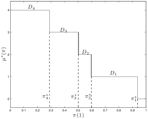
(a) Structured Strategy

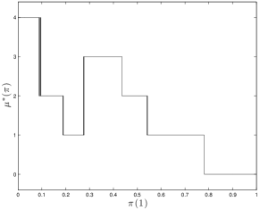
(b) Unstructured Strategy

Figure 1: Optimal sampling strategy $\mu^{*}(\pi)$ for action space $u\in\{0\text{ (announce change) },D_{1}=1,D_{2}=3,\;D_{3}=5,\;D_{4}=10\}$ for a quickest-change detection problem with geometric change time. The noisy observations are from a binary erasure channel and the parameters are specified in Example 1 of Sec.VI. Figure 1(a) depicts a monotone decreasing optimal strategy in posterior $\pi(1)$. Theorem 1 gives sufficient conditions under which the optimal sampling strategy $\mu^{*}(\pi)$ has this structure. The threshold values $\pi_{1}^{*},\pi_{2}^{*},\pi_{3}^{*},\pi_{4}^{*}$ give a finite dimensional characterization of the optimal strategy. Fig.1(b) gives an example where the conditions of Theorem 1 are violated and the optimal strategy is no longer monotone in $\pi(1)$.

Example 2. Sensor Measurement Scheduling: In sensor and radar resource management problems, the sensor is a resource that needs to be allocated amongst several targets [10, 14]. Deploying a sensor to look at a target consumes sensor resources. How should a sensor scheduler decide how often to look at a target in order to detect if the target has made a sudden maneuver (modelled by the Markov chain jumping to a target state)? In radar resource management [13] this is called the revisit time problem.

II Formulation of Optimal Sampling Problem

Let $t=0,1,\ldots$ denote discrete time and $x_{t}$ denote a Markov chain on the finite state space

$$\{e_{1},\ldots,e_{X}\}\text{ where $e_{i}$ is the $X$-dimensional unit vector with 1 in the $i$-th position}.$$ (2)

Here state ‘1’ (corresponding to $e_{1}$) is labelled as the “target state”. Denote

$$\mathbb{X}=\{1,2,\ldots,X\}.$$ (3)

Denote $X\times X$ transition probability matrix $A$ and the $X\times 1$ initial distribution $\pi_{0}$ where

$$A=(A_{ij},i,j\in\mathbb{X}),\;A_{ij}=P(x_{t+1}=e_{j}|x_{t}=e_{i}),\quad\pi_{0}=(\pi_{0}(i),i\in\mathbb{X}),\;\pi_{0}(i)=P(x_{0}=e_{i}).$$ (4)

II-A Measurement Sampling Protocol

Let $\tau_{1},\ldots,\tau_{k-1}$ denote previous discrete time instants at which measurement samples were taken. Let $\tau_{k}$ denote the current time-instant at which a measurement is taken. The measurement sampling protocol proceeds according to the following steps:

Step 1. Observation: A noisy measurement $y_{k}\in\mathbb{Y}$ at time $\tau_{k}$ of the Markov chain is obtained with conditional probability distribution

$$P(y_{k}\leq\bar{y}|x_{\tau_{k}}=e_{x})=\sum_{y\leq\bar{y}}B_{xy},\quad x\in\mathbb{X}$$ (5)

Here $\sum_{y}$ denotes integration with respect to the Lebesgue measure (in which case $\mathbb{Y}\subset\mathbb{R}$ and $B_{xy}$ is the conditional probability density function) or counting measure (in which case $\mathbb{Y}$ is a subset of the integers and $B_{xy}$ is the conditional probability mass function $B_{xy}=P(y_{k}=y|x_{\tau_{k}}=e_{x})$).

Step 2. Sequential Decision Making: Denote the filtration generated by measurements and past decisions (denoted $u_{1},\ldots,u_{k-1}$) as

$$\mathcal{F}_{k}=\text{ $\sigma$-algebra generated by }(y_{1},\ldots,y_{k},u_{1},\ldots,u_{{k-1}}).$$ (6)

At time $\tau_{k}$, a $\mathcal{F}_{k}$ measurable decision $u_{k}\in\mathcal{U}$ is taken where action

$$u_{k} =\mu(\mathcal{F}_{k})\in\mathcal{U}=\{0\text{ (announce change)},1,2,\ldots,L\}$$ (7)

and $$u_{k}=l\text{ denotes: obtain next measurement after }D_{l}\text{ time points},l\in\{1,2,\ldots,L\}.$$

In (7), the strategy $\mu$ belongs to the class of stationary decision strategies denoted $\boldsymbol{\mu}$. Also, $D_{1},\ldots,D_{L}$ are distinct positive integers that denote the set of possible sampling time intervals. Thus the decision $u_{k}$ specifies the next time $\tau_{k+1}$ to make a measurement as follows:

$$\tau_{k+1}=\tau_{k}+D_{u_{k}},\quad u_{k}\in\{1,2,\ldots,L\}.$$ (8)

Step 3. Costs: Associated with the decision $u_{k}\in\mathcal{U}$, a cost $c(x_{t},u_{k})$ is incurred by the decision-maker at each time $t\in[\tau_{k},\ldots,\tau_{k+1}-1]$ until the next measurement is taken at time $\tau_{k}$. Also a non-negative measurement sampling cost $m(x_{\tau_{k}},u_{k})$ is incurred.

Step 4: If $u_{k}=1$, the problem terminates, else set $k$ to $k+1$ and go to Step 1. ∎

Belief State Formulation

It is convenient to re-express Step 2 of the above protocol in terms of the belief state. It is well known from elementary stochastic control [16] that the belief state (posterior) constitutes a sufficient statistic for $\mathcal{F}_{k}$ in (6). Denote the belief state as $\pi_{k}=\mathbb{E}\{x_{\tau_{k}}|\mathcal{F}_{k}\}$. Since the state space (2) comprises of unit indicator vectors, conditional probabilities and conditional expectations coincide. So

$$\pi_{k}=(\pi_{k}(i),\,i\in\mathbb{X})\text{ where }\pi_{k}(i)=P(x_{\tau_{k}}=e_{i}|y_{1},\ldots,y_{k},u_{1},\ldots,u_{{k-1}}),\text{ initialized by }\pi_{0}.$$ (9)

It is easily proved that the belief state is updated via the Bayesian (Hidden Markov Model) filter

$$\pi_{k} =T(\pi_{k-1},y_{k},u_{k-1}),\text{ where }T(\pi,y,u)=\frac{B_{y}({A^{\prime}})^{D_{u}}\pi}{\sigma(\pi,y,u)},\;\sigma(\pi,y,u)=\mathbf{1}_{X}^{\prime}B_{y}({A^{\prime}})^{D_{u}}\pi$$ (10)

$$B_{y} =\text{diag}(P(y|x),x\in\mathbb{X}).$$

Here $\sigma(\pi,y,u)$ is the normalization measure of the Bayesian update with $\sum_{y}\sigma(\pi,y,u)=1$. Also $\mathbf{1}_{X}$ denotes the $X$ dimensional vector of ones. Note that $\pi$ in (10) is an $X$-dimensional probability vector. It belongs to the $X-1$ dimensional unit-simplex denoted as

$$\Pi(X)\stackrel{{\scriptstyle\triangle}}{{=}}\left\{\pi\in\mathbb{R}^{X}:\mathbf{1}_{X}^{\prime}\pi=1,\quad 0\leq\pi(i)\leq 1\text{ for all }i\in\mathbb{X}\right\}$$ (11)

For example, $\Pi(2)$ is a one dimensional simplex (unit line segment), $\Pi(3)$ is a two-dimensional simplex (equilateral triangle); $\Pi(4)$ is a tetrahedron, etc. Note that the unit vector states $e_{1},e_{2},\ldots,e_{X}$ defined in (2) of the Markov chain $x$ are the vertices of $\Pi(X)$.

Step 2 in the above protocol expressed in terms of the belief state reads: At decision time $\tau_{k}$

• Step 2(a). Update belief state $\pi_{k}$ according to Bayesian filter (10)

• Step 2(b). Make decision $u_{k}\in\mathcal{U}$ using stationary strategy $\mu$ as (see (7))

  $$u_{k}=\mu(\pi_{k})\in\mathcal{U}=\{0\text{ (announce change)},1,2,\ldots,L\}.$$ (12)

II-B Sequential Decision-maker’s Objective and Stochastic Dynamic Programming

Given the above protocol with measurement-sampling strategy $\mu$ in (12), we now define the objective of the sequential decision maker. Let $(\Omega,\mathcal{F})$ be the underlying measurable space where $\Omega=(\mathbb{X}\times\mathcal{U}\times\mathbb{Y})^{\infty}$ is the product space, which is endowed with the product topology and $\mathcal{F}$ is the corresponding product sigma-algebra. For any $\pi_{0}\in\Pi(X)$, and strategy $\mu\in\boldsymbol{\mu}$, there exists a (unique) probability measure $\mathbb{P}^{\mu}_{\pi_{0}}$ on $(\Omega,\mathcal{F})$, see [7] for details. Let $\mathbb{E}^{\mu}_{\pi_{0}}$ denote the expectation with respect to the measure $\mathbb{P}^{\mu}_{\pi_{0}}$.

Define the $\{\mathcal{F}_{k},k\geq 1\}$ measurable stopping time $k^{*}$ as

$$k^{*}=\{\inf k:u_{k}=0\text{ (announce target state and stop) }\}.$$ (13)

That is, $k^{*}$ is the time at which the decision maker declares the target state has been reached and the problem terminates. For each initial distribution $\pi_{0}\in\Pi(X)$, and strategy $\mu$, the decision maker’s global objective function is

$$J_{\mu}(\pi_{0})=\mathbb{E}^{\mu}_{\pi_{0}}\left\{\sum_{k=1}^{k^{*}-1}\left[m(x_{\tau_{k}},u_{k})+\sum_{t=\tau_{k}}^{\tau_{k+1}-1}c(x_{t},u_{k})\right]+c(x_{{\tau_{k^{*}}}},u_{{k^{*}}})\right\}$$ (14)

Recall that $c(x,u)$ and measurement sampling cost $m(x,u)$ are defined in Step 3 of the protocol. Using the smoothing property of conditional expectations, (14) can be expressed in terms of the belief state $\pi$ as

$$J_{\mu}(\pi_{0}) =\mathbb{E}^{\mu}_{\pi_{0}}\left\{\sum_{k=1}^{k^{*}-1}C(\pi_{k},u_{k})+C(\pi_{{{k^{*}}}},u_{{k^{*}}}=0)\right\}$$ (15)

$$\text{ where }C(\pi,u) =C_{u}^{\prime}\pi\text{ for }u\in\mathcal{U},\;\text{ and the $X$-dimensional cost vector $C_{u}$ is }$$

$$C_{0} =\begin{bmatrix}c(e_{1},0),\ldots,c(e_{X},0)\end{bmatrix}^{\prime},$$

$$C_{u} =m_{u}+(I+A+\cdots+A^{D_{u}-1})c_{u}\text{ for }u\in\{1,2,\ldots,L\},$$

$$c_{u} =\begin{bmatrix}c(e_{1},u),\ldots,c(e_{X},u)\end{bmatrix}^{\prime},\quad m_{u}=\begin{bmatrix}m(e_{1},u),\ldots,m(e_{X},u)\end{bmatrix}^{\prime}.$$

The decision-maker aims to determine the optimal strategy $\mu^{*}\in\boldsymbol{\mu}$ to minimize (15), i.e.,

$$J_{\mu^{*}}(\pi_{0})=\inf_{\mu\in\boldsymbol{\mu}}J_{\mu}(\pi_{0}).$$ (16)

The existence of an optimal stationary strategy $\mu^{*}$ follows from [4, Prop.1.3, Chapter 3].

Considering the global objective (15), the optimal stationary strategy $\mu^{*}:\Pi(X)\rightarrow\mathcal{U}$ and associated optimal objective $J_{\mu^{*}}(\pi)$ are the solution of the following “Bellman’s stochastic dynamic programming equation”

$$\mu^{*}(\pi) =\arg\min_{u\in\mathcal{U}}Q(\pi,u),\;J_{\mu^{*}}(\pi)=V(\pi)=\min_{u\in\mathcal{U}}Q(\pi,u),$$ (17)

$$\text{ where }Q(\pi,u) =C(\pi,u)+\sum_{y\in\mathbb{Y}}V\left(T(\pi,y,u)\right)\sigma(\pi,y,u),\;u=1,\ldots,L,\quad Q(\pi,0)=C(\pi,0).$$

Recall $T(\pi,y,u)$ and $\sigma(\pi,y,u)$ were defined in (10). The above formulation is a generalization of a partially observed Markov decision process (POMDP), since POMDPs assume finite observations spaces $\mathbb{Y}$ while in our formulation $\mathbb{Y}$ can be discrete or continuous (see (5)).

Define the set of belief states where it is optimal to apply action $u=0$ as

$$\mathcal{S}=\{\pi\in\Pi(X):\mu^{*}(\pi)=0\}=\{\pi\in\Pi(X):Q(\pi,0)\leq Q(\pi,u),\;u\in\{1,2,\ldots,L\}\}$$ (18)

$\mathcal{S}$ is called the stopping set since it is the set of belief states to “declare target state and stop”.

Since the belief state space $\Pi(X)$ is an uncountable, Bellman’s equation (17) does not translate directly into numerical algorithms. However, in subsequent sections, we exploit the structure of Bellman’s equation to prove various structural results about the optimal strategy $\mu^{*}$ using lattice programming and stochastic dominance tools.

II-C Example: Quickest Change Detection with Measurement Control

We now formulate the quickest detection problem with optimal sampling – this serves as a useful example to illustrate the above general model. Before proceeding, it is important to recall that in our model, decisions (whether to stop, or continue and take next observation sample after $D_{l}$ time points) are made at times $\tau_{1},\tau_{2},\ldots$. In contrast, the state of the Markov chain (which models the change we want to detect) can change at any time $t$. We need to construct the delay penalty and false alarm penalties carefully to take this into account.
1. Phase-Distributed (PH) Change time: In quickest detection, the target state (which we label as state 1 by convention) is an absorbing state. States $2,\ldots,X$ (corresponding to unit vectors $e_{2},\ldots,e_{X}$) are now fictitious states that form a single composite state that the Markov chain $x_{t}$ resides in before jumping into the target absorbing state. So the transition matrix (4) is

$$A=\begin{bmatrix}1&0\\ \underline{A}_{(X-1)\times 1}&\bar{A}_{(X-1)\times(X-1)}\end{bmatrix}.$$ (19)

The “change time” $t^{*}$ denotes the time at which $x_{t}$ enters the absorbing state 1, i.e.,

$$t^{*}=\inf\{t>0:x_{t}=1\}.$$ (20)

Of course, in the special case when $x$ is a 2-state Markov chain (i.e., $X=2$), the change time $t^{*}$ in (20) is geometrically distributed.
For the multi-state case, to ensure that $t^{*}$ is finite, assume states $2,3,\ldots X$ are transient. This is equivalent to $\bar{A}$ in (19) satisfying $\sum_{n=1}^{\infty}\bar{A}^{n}_{ii}<\infty$ for $i=1,\ldots,X-1$ (where $\bar{A}^{n}_{ii}$ denotes the $(i,i)$ element of the $n$-th power of matrix $\bar{A}$). With the transition probabilities (19), the distribution of the change time $t^{*}$ is given by the PH-distribution

$$P(t^{*}=0)=\pi_{0}(1),\quad P(t^{*}=t)=\bar{\pi}_{0}^{\prime}\bar{A}^{t-1}\underline{A},\quad t\geq 1$$ (21)

where $\bar{\pi}_{0}=[\pi_{0}(2),\ldots,\pi_{0}(X)]^{\prime}$. By choosing $(\pi_{0},A)$ and state space dimension $X$, one can approximate any given change-time distribution on $[0,\infty)$ by PH-distribution (21); see [18, pp.240-243]. Indeed, PH-distributions form a dense subset for the set of all distributions.
2. Observations: Since states $2,3,.\ldots,X$ are fictitious states that shape the PH-distributed change time (21), they are indistinguishable in terms of the observation $y$. That is, $B_{2y}=B_{3y}=\cdots=B_{Xy}$ for all $y\in\mathbb{Y}$.
3. Costs: Associated with the quickest detection problem are the following costs.
(i) False Alarm: Let $k^{*}$ denote the time $\tau_{k}$ at which decision $u_{k}=0$ (stop and announce target state) is chosen, so that the problem terminates. If the decision to stop is made before the Markov chain reaches the target state 1, i.e., $k^{*}<t^{*}$, then a false alarm penalty ${f}$ is paid. So the false alarm penalty is ${f}\sum_{i\neq 1}I(x_{\tau_{k}}=e_{i},u_{k}=1)$ where ${f}$ is a user defined non-negative constant. The expected false alarm penalty based on the accumulated history is

$$\sum_{i\neq 1}{f}\mathbb{E}\{I(x_{\tau_{k}}=e_{i},u_{k}=1)|\mathcal{F}_{k}\}={f}(\mathbf{1}_{X}-e_{1})^{\prime}\pi_{k}I(u_{k}=1).$$ (22)

Recall $\mathbf{1}_{X}$ denotes the $X$-dimensional vector of ones.
(ii) Delay cost of continuing: Suppose decision $u_{k}\in\{1,2,\ldots,L\}$ is taken at time $\tau_{k}$. So the next sampling time is $\tau_{k+1}=\tau_{k}+D_{u_{k}}$. Then for any time $t\in[\tau_{k},\tau_{k+1}-1]$, the event $\{x_{t}=e_{1},u_{k}\}$ signifies that a change has occurred but not been announced by the decision maker. Since the decision maker can make the next decision (to stop or continue) at $\tau_{k+1}$, the delay cost incurred in the time interval $[\tau_{k},\tau_{k+1}-1]$ is $d\sum_{t=\tau_{k}}^{\tau_{k+1}-1}I(x_{t}=e_{1},u_{k})$ where $d$ is a non-negative constant. The expected delay cost in interval $[\tau_{k},\tau_{k+1}-1]=[\tau_{k},\tau_{k}+D_{u_{k}}-1]$ is

$$d\sum_{t=\tau_{k}}^{\tau_{k+1}-1}\mathbb{E}\{I(x_{t}=e_{1},u_{k})|\mathcal{F}_{k}\}=de_{1}^{\prime}(I+A+\cdots+A^{D_{u_{k}}-1})^{\prime}\pi_{k},\quad u_{k}\in\{1,2,\ldots,L\}.$$ (23)

(iii) Measurement Sampling Cost: Suppose decision $u_{k}\in\{1,2,\ldots,L\}$ is taken at time $\tau_{k}$. As in (15) let $m_{u_{k}}=(m(x_{\tau_{k}}=e_{i},u_{k}),i\in\mathbb{X})$ denote the non-negative measurement cost vector for choosing to take a measurement. For convenience, assume the measurement cost when choosing $u=0$ (stop) is zero. Next, since in quickest detection, states $2,\ldots,X$ are fictitious states that are indistinguishable in terms of cost, choose $m(e_{2},u)=\ldots=m(e_{X},u)$.
Examples of measurement sampling costs are:
(a) $m(e_{i},u)$ is independent of state $i$ and action $u$. This simple choice of a constant measurement cost at each time, still results in non-trivial global costs for the decision maker since this cost is incurred each time a measurement is made – so choosing a decision $u$ with smaller sampling delay will result in more measurements until the final decision to stop, thereby incurring a higher total measurement cost for the global decision maker.
(b) $m(e_{i},u)$ is decreasing in $u$ for $u\neq 0$. Choosing $m(e_{i},u)$ to decrease in $u$ penalizes choosing small sampling intervals even more than a constant cost.

Summary and Kolmogorov–Shiryayev criterion: To summarize, the costs $C(\pi,u)$ for quickest detection with optimal sampling and PH-distributed change time are

$$C(\pi,0) ={f}(\mathbf{1}_{X}-e_{1})^{\prime}\pi,\quad C(\pi,u)=c_{u}^{\prime}\pi+m_{u}^{\prime}\pi,\text{ for }u\in\{1,2,\ldots,L\},$$

where $$c_{u}=d(I+A+\cdots+A^{D_{u}-1})e_{1}.$$ (24)

For constant measurement cost $m(x,u)=m$, $u\in\{1,2,\ldots,L\}$, the quickest detection optimal sampling objective (15) with costs (24) can be expressed as

$$J_{\mu}(\pi_{0})=d\mathbb{E}^{\mu}_{\pi_{0}}\{(k^{*}-t^{*})^{+}\}+{f}\mathbb{P}^{\mu}_{\pi_{0}}(k^{*}<t^{*})+m\sum_{u=1}^{L}\sum_{k:\tau_{k}\leq k^{*}}\mathbb{P}^{\mu}_{\pi_{0}}(u_{k}=u)$$ (25)

where the PH-distributed change time $t^{*}$ and $k^{*}$ are defined in (20), (13). For the special case $\mathcal{U}=\{0\text{ (stop)},D_{1}=1\}$, measurement cost $m_{u}=0$, geometrically distributed $t^{*}$ (so $X=2$), then (25) becomes the Kolmogorov–Shiryayev criterion for detection of disorder [22].

III Structural Results for Optimal Sampling Policy $\mu^{*}(\pi)$ for 2-state case

This section analyzes the structure of the optimal sampling strategy $\mu^{*}(\pi)$ (solution of Bellman’s equation (17)) for two-state Markov chains ($X=2$). Recall that two-state Markov chains model geometric distributed change times in quickest detection problems.

We list the following assumptions that will be used in this section.

• (i) The costs $C(e_{i},u)$ in (15) are increasing with $i\in\mathbb{X}$ for each $u\in\mathcal{U}$.
  (ii) The target state $e_{1}$ belongs to the stopping set $\mathcal{S}$ defined in (18).

• The transition matrix $A$ is totally positive of order 2 (TP2). That is, all second order minors are non-negative.

• The observation matrix $B$ is TP2.

• $C(e_{i},u)$ is submodular for $u\in\{1,2,\ldots,L\}$, that is $C(e_{i},u+1)-C(e_{i},u)$ is decreasing in $i\in\mathbb{X}$.

Consider the following assumption where $A^{D_{u}}|_{ij}$ denotes the $(i,j)$ element of matrix $A^{D_{u}}$:

• For each $q\in\mathbb{X}$, $\sum_{j\geq q}A^{D_{u}}|_{ij}$ is submodular. That is, $\sum_{j\geq q}A^{D_{u+1}}|_{ij}-A^{D_{u}}|_{ij}$ is decreasing in $i\in\mathbb{X}$ for $u=1,2,\ldots,L-1$.

• $A^{D_{u}}|_{22}$ and $A^{D_{u}}|_{12}$ is decreasing in $u\in\{1,2,\ldots,L\}$.

These assumptions are discussed below in Sec.III-B and hold for quickest detection problems.

III-A Optimality of Threshold Policy for Sequential Optimal Sampling

Note that for a 2-state Markov chain ($X=2$), the belief state space $\Pi(X)$ is the one dimensional simplex $\pi(1)+\pi(2)=1$. So it suffices to represent $\pi$ by its first element $\pi(1)$.

Theorem 1

Consider the optimal sampling problem of Sec.II with state dimension $X=2$ and action space $\mathcal{U}$ (7). Then the optimal strategy $\mu^{*}(\pi)$ in (17) has the following structure:
(i) The optimal stopping set $\mathcal{S}$ (18) is a convex subset of $\Pi(X)$. Therefore under (A0), the stopping set is the interval $\mathcal{S}=(\pi_{1}^{*},1]$ where the threshold $\pi^{*}\in[0,1]$.
(ii) Under assumptions (A1-A5), the optimal sampling strategy $\mu^{*}(\pi)$ in (17) is decreasing with $\pi(1)$. Thus, there exist up to $L$ thresholds denoted $\pi_{1}^{*},\ldots,\pi_{L}^{*}$ with $0\leq\pi_{L}^{*}\leq\pi_{L-1}^{*}\leq\cdots\leq\pi_{1}^{*}\leq 1$ such that the optimal strategy satisfies

$$\mu^{*}(\pi)=\begin{cases}L\text{ (sample after $D_{L}$ time points) }&\text{ if }0\leq\pi(1)<\pi_{L}^{*}\\ {L-1}\text{ (sample after $D_{L-1}$ time points) }&\text{ if }\pi_{L}^{*}\leq\pi(1)<\pi_{L-1}^{*}\\ \vdots&\vdots\\ 1\text{ (sample after $D_{1}$ time points) }&\text{ if }\pi_{2}^{*}\leq\pi(1)<\pi_{1}^{*}\\ 0\text{ (announce change )}&\text{ if }\pi_{1}^{*}\leq\pi(1)\leq 1\end{cases}$$ (26)

where the sampling delays are ordered as $D_{1}<D_{2}<\ldots<D_{L}$.

The proof of Theorem 1 is in Appendix -B. As an example, consider quickest detection with optimal sampling for geometric distributed change time. From (19), the transition matrix is $A=\begin{bmatrix}1&0\\ 1-A_{22}&A_{22}\end{bmatrix}$ and expected change time is $\mathbb{E}\{t^{*}\}=\frac{1}{1-A_{22}}$ where $t^{*}$ is defined in (20).

Theorem 2

Consider the quickest detection problem with optimal sampling and geometric-distributed change time formulated in Sec.II-C with costs defined in (24). Assume the measurement cost $m(x,u)$ satisfies (A1) and (A4), e.g., the measurement cost is a constant. Then if (A3) holds, Theorem 1 holds. So the optimal sampling strategy (26) makes measurements less frequently when away from the target state and more frequently when closer to the target state. (Note, (A1)(ii), (A2), (A5) hold automatically and no assumptions are required on the delay or stopping costs in (24)).

There are two main conclusions regarding Theorem 2. First, for constant measurement cost, Theorem 2 holds without any assumptions for Gaussians, exponentials, and several other classes of observation distributions that satisfy (A3). Second, the optimal strategy $\mu^{*}(\pi)$ is monotone in posterior $\pi(1)$ and therefore has a finite dimensional characterization. To determine the optimal strategy, one only needs to determine (estimate) the values of the $L$ thresholds $\pi_{1}^{*},\ldots,\pi_{L}^{*}$. These can be estimated via a simulation-based stochastic optimization algorithm. We will give bounds for these threshold values in Sec.IV. Fig.1 illustrates such a monotone policy.

A short word on the proof presented in Appendix -B. It involves analyzing the structure of Bellman’s equation (17). It will be shown that $Q(\pi,u)$ in (17) is a submodular function (defined in Appendix -B) on the partially ordered set $[\Pi(X),\geq_{r}]$ which constitutes a lattice. Here $\geq_{r}$ denotes the monotone likelihood ratio stochastic order defined in Sec.V-C. For $X=2$, $\Pi(X)$ is the unit interval [0,1] and in this case $[\Pi(X),\geq_{r}]$ is a chain (totally ordered set) and $\geq_{r}$ is equivalent to first order stochastic dominance. For $X\geq 2$ considered in the next section, a similar idea is used to bound the optimal policy on $[\Pi(X),\geq_{r}]$.

Remark: Interpretation of [3]. We comment here briefly on the recent paper [3] which considers quickest detection with measurement control where at each time the decision is made whether to take a measurement or not. This can be formulated as our optimal sampling problem by considering the action space $\mathcal{U}=\{0\text{ (announce change)},D_{1},D_{2},\ldots,D_{L}\}$ with sampling interval $D_{i}=i$ and $L$ chosen sufficiently large. In [3], a different action space is chosen, namely $\{0\text{ (announce change)},m\text{ (take measurement)},\bar{m}\text{ (no measurement)}\}$. With this action space, [3] shows that the optimal strategy is not necessarily monotone in the posterior. $\pi$. However, with the action space $\mathcal{U}$ defined above, Theorem 2 shows that the optimal strategy indeed is monotone.

We can interpret the non-monotone optimal strategy in [3] as follows. Our action 1 (sample next point) corresponds to action $m$ in [3], action 2 (sample after 2 points) corresponds to $(\bar{m},m)$, action 3 (sample after 3 points) corresponds to $(\bar{m},\bar{m},m)$, etc. Reading off the monotone optimal strategy $\mu^{*}(\pi)\in\{3,2,1\}$ versus $\pi$ using the action space of [3] yields strategy $\{\bar{m},\bar{m},m,\bar{m},m,m\}$ which is non-monotone, due to presence of the action $\bar{m}$ sandwiched between two $m$’s.

III-B Discussion of Assumptions A1-A5

To illustrate the assumptions of Theorem 1, we will now prove Theorem 2 by showing that assumptions that (A1-A5) hold. Recall from (19) that for quickest detection with geometric change time, the transition matrix is

$$A=\begin{bmatrix}1&0\\ 1-A_{22}&A_{22}\end{bmatrix}.\text{ So }\;A^{D_{u}}=\begin{bmatrix}1&0\\ 1-A^{D_{u}}_{22}&A^{D_{u}}_{22}\end{bmatrix}.$$ (27)

III-B1 Assumption (A1)(i)

This requires the elements of the cost vector to be increasing. However, in quickest detection, the instantaneous cost $c(e_{i},u)$ for $u\geq 1$ defined in (24) is decreasing in $i$ if the measurement cost $m$ is a constant. But all is not lost. Remarkably, a clever transformation can be applied to make a transformed version of the cost increase with $i$ and yet ensure (A4) holds and keep the optimal strategy unchanged! This transformation is crucial for proving Theorem 2, particularly for constant measurement cost. (Assuming a measurement cost increasing in the state $i$ makes the proof easier but may be unrealistic in applications). We define this transformation via the following theorem - it exploits the special structure of the quickest detection problem.

Theorem 3

Consider the quickest time detection problem with costs defined in (24). Assume the sampling cost $m(e_{i},u)$ is a constant. Define the transformed costs $\underline{C}(\pi,u)$ as follows:

$$\underline{C}(\pi,0) =C(\pi,0)-\alpha C(\pi,L),$$

$$\underline{C}(\pi,u) =C(\pi,u)-\alpha C(\pi,L)+\alpha\sum_{y}C(T(\pi,y,u),L)\sigma(\pi,y,u),\quad u\in\{1,2,\ldots,L\}$$ (28)

for any constant $\alpha\in\mathbb{R}$. Then:
(i) Bellman’s equation (17) applied to optimize the global objective (15) with transformed costs $\underline{C}(\pi,u)$ yields the same optimal strategy $\mu^{*}(\pi)$ as the global objective with original costs $C(\pi,u)$.
(ii) Choosing $\alpha=1/(1-A_{22}^{D_{u}})$ implies $\underline{C}(e_{i},u)$ satisfies (A1) and (A4). ∎

Theorem 3 is proved in Appendix -C. It asserts that the transformed costs $\underline{C}(e_{i},u)$ satisfies (A1) and (A4) even for constant measurement cost. Therefore Theorem 1 holds and the optimal strategy for the transformed costs is monotone in the posterior distribution. Note that Theorem 3 also says that the optimal strategy $\mu^{*}(\pi)$ is unchanged by this transformation. Thus Theorem 1 holds for the original quickest detection costs, thereby proving Theorem 2.

Assumption (A1)(ii) is natural for the stopping problem to be well defined. It says that if it was known with certainty that the target state $e_{1}$ has been reached, then it is optimal to stop. For quickest time detection it holds trivially since $C(e_{1},0)\leq C(\pi,u)$ for $u\in\{1,\ldots,L\},\pi\in\Pi(X)$.

III-B2 Assumption (A2)

From the structure of transition matrix $A$ in (27), clearly (A2) holds automatically for the quickest detection problem. For numerous examples of TP2 transition matrices, see [9]. Also, $A$ does not need to have an absorbing state for Theorem 1 to hold.

III-B3 Assumption (A3)

Numerous continuous and discrete noise distributions satisfy the TP2 property, see [9]. Examples include Gaussians, Exponential, Binomial, Poisson, etc. Examples of discrete observation distribution satisfying (A3) include binary erasure channels – see Sec.VI. A binary symmetric channel with error probability less than 0.5 also satisfies (A3).

III-B4 Assumption (A4)

In general Theorem 1 requires the costs $C(e_{i},u)$ to be submodular. However, for the special case of quickest detection with optimal sampling, from Theorem 3 shows that only the measurement cost $m(e_{i},u)$ needs to be submodular, i.e., $m(e_{i},u+1)-m(e_{i},u)$ is decreasing in $i$. This holds trivially if the measurement cost is independent of the state.

III-B5 Assumption (A5)

This is a submodularity condition on the transition matrix. Since from (27) $A^{D_{u}}|_{21}=0$ and $A^{D_{u}}|_{22}=A_{22}^{D_{u}}$, clearly (A5) holds automatically for the quickest detection problem with optimal sampling.

IV Myopic Bounds to Optimal Strategy for multi-state Markov Chain

This section considers the optimal sampling problem for multi-state Markov chains ($X\geq 2$). Recall that multi-state Markov chains can model PH-distributed change times (19) in quickest detection problems. Theorems 4 and 5 are the main results of this section. They characterize the structure of optimal strategy $\mu^{*}(\pi)$ which is the solution of Bellman’s equation (17).

Define the following ordering of two arbitrary transition matrices $A^{(1)}$ and $A^{(2)}$:

$$A^{(1)}\succeq A^{(2)}\text{ if }A^{(1)}_{ij}A^{(2)}_{m,j+1}\leq A^{(2)}_{ij}A^{(1)}_{m,j+1},\quad i,j+1,m\in\mathbb{X}.$$ (29)

The following are the main assumptions used in this section:

• The transition matrix satisfies $A\succeq A^{2}$ where the ordering $\succeq$ is defined in (29).

• There exist a positive constant $\alpha$ satisfying
  (i) $\alpha\geq f/(d(1-A_{21}))$
  (ii) $\sum_{l=1}^{D_{u}-1}A^{l}|_{i1}+\alpha(A_{i1}-A^{D_{u}+1}|_{i1})$ decreasing in $i=2,\ldots,X$.

(A6) and (A7) are discussed at the end of this section. (A6) and (A7) hold trivially for the two state Markov chain case ($X=2$) with absorbing state when $A$ is of the form (27). Examples for $X\geq 3$ are given in Sec.VI.

IV-A Myopic Lower Bound to Optimal Policy

For multi-state Markov chain observed in noise, determining sufficient conditions for the optimal strategy to have a monotone structure is an open problem. In this section we show that the optimal sampling strategy $\mu^{*}(\pi)$ is lower bounded by a myopic strategy. Define the myopic strategy ${\underline{\mu}}(\pi)$ and myopic stopping set $\underline{\mathcal{S}}$ by

$${\underline{\mu}}(\pi) =\arg\min_{u\in\mathcal{U}}C(\pi,u)$$

$$\underline{\mathcal{S}}=\{\pi\in\Pi(X):\underline{\mu}^{*}(\pi)=0\} =\{\pi\in\Pi(X):C(\pi,0)<C(\pi,u),\;u\in\{1,2,\ldots,L\}\}$$ (30)

So $\underline{\mathcal{S}}$ is the set of belief states for which the myopic strategy declares stop.

The following is the main result of this section. The proof is in Appendix -D.

Theorem 4

Consider the sequential sampling problem of Sec.II with optimal strategy specified by (17). Then

1. The stopping set $\mathcal{S}$ defined in (18) is a convex subset of the belief state space $\Pi(X)$.

2. $\underline{\mathcal{S}}\subset\mathcal{S}$ where $\underline{\mathcal{S}}$ is the myopic stopping set defined in (30).

3. Under (A1), (A2), (A3), (A6), the myopic strategy ${\underline{\mu}}(\pi)$ defined in (30) forms a lower bound for the optimal strategy $\mu^{*}(\pi)$, i.e., $\mu^{*}(\pi)\geq{\underline{\mu}}(\pi)$ for all $\pi\in\Pi(X)-\mathcal{S}$.

4. If (A4) holds, then the myopic strategy is ${\underline{\mu}}(\pi)$ is increasing with $\pi$ (with respect to the monotone likelihood ratio (MLR) stochastic order to be defined in Sec.V-C).

The above theorem says that the myopic strategy ${\underline{\mu}}(\pi)$ comprising of increasing step functions lower bounds the optimal strategy $\mu^{*}(\pi)$. The myopic strategy specified by (30) is computed trivially on the simplex $\Pi(X)$. Therefore, the above theorem gives a useful lower bound ${\underline{\mu}}(\pi)$ for the optimal strategy $\mu^{*}(\pi)$ (which is intractable to compute). Also since ${\underline{\mu}}(\pi)$ is sub-optimal, it incurs a higher cost compared to the optimal strategy. This cost associated with ${\underline{\mu}}(\pi)$ can be evaluated by simulation and forms an upper bound to the optimal achievable cost.

IV-B Quickest Detection with Optimal Sampling for PH-Distributed Change Time

We now use Theorem 4 to construct a myopic strategy that upper bounds the optimal strategy for quickest detection with sampling for PH-distributed change time. However, (A1) does not hold for the quickest detection costs $C(\pi,u)$ in (24) To proceed, it is convenient to define the following transformed cost $\bar{C}(\pi,u)$ and myopic strategy $\bar{\mu}(\pi)$:

$$\bar{C}(\pi,0) =C(\pi,0)+\alpha de_{1}^{\prime}A^{\prime}\pi,$$ (31)

$$\bar{C}(\pi,u) =C(\pi,u)+\alpha de_{1}^{\prime}A^{\prime}\pi-\alpha de_{1}^{\prime}{A^{\prime}}^{D_{u}+1}\pi,\quad u\in\{1,2,\ldots,L\},$$

$$\quad\bar{\mu}(\pi) =\arg\min_{u\in\{1,2,\ldots,L\}}\bar{C}(\pi,u).$$

It will be shown in the proof of the theorem below, that the optimal strategy for global objective (15) with these transformed costs $\bar{C}(\pi,u)$ remains unchanged and is still $\mu^{*}(\pi)$.

The main result regarding quickest detection with optimal sampling for PH-distributed change times is as follows. The proof is in Appendix -E.

Theorem 5

Consider the quickest detection optimal sampling problem for PH-distributed change time ($X\geq 2$) defined in Sec.II-C with costs in (24) and transformed costs (31). Then

1. The optimal stopping set $\mathcal{S}$ (18) is a convex subset of the belief state space $\Pi(X)$ and contains $e_{1}$.

2. The optimal stopping set is lower bounded by the myopic stopping set $\underline{\mathcal{S}}$ in (30), i.e., $\underline{\mathcal{S}}\subset\mathcal{S}$.

3. Under (A2), (A3), (A6), (A7), for $\pi\in\Pi(X)-\underline{\mathcal{S}}$, the myopic strategy $\bar{\mu}(\pi)$ in (31) upper bounds the optimal strategy, i.e., $\bar{\mu}(\pi)\geq\mu^{*}(\pi)\text{ for all }\pi\in\Pi(X)-\underline{\mathcal{S}}$. Moreover, $\bar{\mu}(\pi)$ is increasing in $\pi$ with respect to the MLR order.

4. For the case of geometrically distributed change time ($X=2$), (A2) and (A6) hold automatically. So if (A3) holds and $\alpha$ is chosen according to (A7)(i), then $\bar{\mu}(\pi)\geq\mu^{*}(\pi)$ for all $\pi\in\Pi(X)$. Also $\bar{\mu}(\pi)$ is decreasing in $\pi(1)$.

Discussion: Theorem 5 gives a lot of analytical mileage in terms of bounding the optimal strategy. Statements (1) characterizes the convexity of the stopping set and Statement (2) lower bounds $\mathcal{S}$. Statement (3) asserts that the optimal sampling strategy $\mu^{*}$ can be upper bounded for PH-distributed change times by the myopic strategy $\bar{\mu}$.

Statement (4) shows that for geometrically distributed change times, the bounds on $\mu^{*}$ and $\mathcal{S}$ apply without requiring any assumptions apart from that on the observation distribution (A3). In particular, Statement (4) together with Theorem 2 say that the optimal strategy $\mu^{*}(\pi)$ is monotone in $\pi(1)$, and upper bounds for the threshold values $\pi_{1}^{*},\pi_{2}^{*},\ldots,\pi_{L}^{*}$ can be constructed using the myopic strategy $\bar{\mu}(\pi)$. Therefore these upper bounds can be used to initialize a stochastic optimization algorithm to estimate the thresholds of the optimal monotone policy.

Discussion of Assumptions (A6) and (A7): (A6) is a sufficient to preserve monotone likelihood ratio (MLR) dominance of the belief state with a one-step predictor. MLR stochastic order $\geq_{r}$ is defined in Sec.V-C. (A6) ensures that if two belief states satisfy $\pi_{1}\geq_{r}\pi_{2}$, then the one-step ahead Bayesian predictor satisfies $A^{\prime}\pi_{1}\geq_{r}A^{\prime}\pi_{2}$. Theorem 9 in Sec.V-C analyzes this and other stochastic dominance properties of Bayesian filters and predictors that are crucial to prove the results of this paper.

(A7) is sufficient for the transformed cost $\bar{C}(\pi,u)$ defined in (31) to satisfy the following: $-\bar{C}(\pi,u)$ satisfies (A1) and $\bar{C}(\pi,u)$ to satisfies (A4). The fact that $\bar{C}(\pi,u)$ is decreasing (since its negative satisfies (A1)), gives an upper bound by a proof completely analogous to Theorem 4.

V Performance and Sensitivity of Optimal Strategy

In previous sections, we have presented structural results on monotone optimal strategies. In comparison, this section focuses on achievable costs attained by the optimal strategy. This section presents two results. First, we give bounds on the achievable performance of the optimal strategies by the decision maker. This is done by introducing a partial ordering of the transition and observation probabilities – the larger these parameters with respect to this order, the larger the optimal cost incurred. Thus we can compare models and bound the achievable performance of a computationally intractable problem. Second, we give explicit bounds on the sensitivity of the total sampling cost with respect to sampling model – this bound can be expressed in terms of the Kullback-Leibler divergence. Such a robustness result is useful since even if a model violates the assumptions of the previous section, as long as the model is sufficiently close to a model that satisfies the conditions, then the optimal strategy is close to a monotone strategy.

V-A How does total cost of the optimal sampling strategy depend on state dynamics?

Consider the optimal sampling problem formulated in Sec.II. How does the optimal expected cost $J_{\mu^{*}}$ defined in (16) vary with transition matrix $A$ and observation matrix $B$? In particular, is it possible to devise an ordering for transition matrices and observation distributions such that the larger they are, the smaller the optimal sampling cost? Such a result would allow us to compare the optimal performance of different sampling models, even though computing these is intractable. Moreover, characterizing how the optimal achievable cost varies with transition matrix and observation distribution is useful. Recall in quickest detection the transition matrix specifies the change time distribution. In sensor scheduling applications the transition matrix specifies the mobility of the state. The observation matrix specifies the noise distribution.

Consider two distinct models $\theta=(A,B)$ and $\bar{\theta}=(\bar{A},\bar{B})$ of the optimal sampling problem where $A,\bar{A}$ are transition matrices and $B,\bar{B}$ are observation matrices. Let $\mu^{*}(\theta)$ and $\mu^{*}({\bar{\theta}})$ denote, respectively, the optimal strategies for these two different models. Let $J_{\mu^{*}(\theta)}(\pi;\theta)=V(\pi;\theta)$ and $J_{\mu^{*}(\bar{\theta})}(\pi;\bar{\theta})=V(\pi;\bar{\theta})$ denote the optimal value functions in (17) corresponding to applying the respective optimal strategies. Recall also that the costs in (15) depend on the transition matrix $A$. So we will use the notation $C(\pi,u;\theta)$ and $C(\pi,u;\bar{\theta})$ to make the dependence of the cost on the transition matrix explicit.

Introduce the following reverse Blackwell ordering [21] of observation distributions. Let $B$ and $\bar{B}$ denote two observation distributions defined as in (5). Then $\bar{B}$ reverse Blackwell dominates $B$ denoted as

$$\bar{B}\succeq_{B}B\text{ if }\bar{B}=BR$$ (32)

where $R=(R_{lm})$ is a stochastic kernel, i.e., $\sum_{m}R_{lm}=1$. This means that $B$ yields more accurate measurements of the underlying state than $\bar{B}$.

The question we pose is: How does the optimal cost $J_{\mu^{*}(\theta)}(\pi;\theta)$ vary with transition matrix $A$ and observation distribution $B$? For example, in the quickest detection optimal sampling problem, do certain phase-type distributions result in larger total optimal cost compared to other phase-type distributions?

Theorem 6

Consider two optimal sampling problems with models $\theta=(A,B)$ and $\bar{\theta}=(\bar{A},\bar{B})$, respectively. Assume ${A}\succeq\bar{A}$ with respect to ordering (29), $B\succeq_{B}\bar{B}$ with respect to ordering (32), and (A1), (A2), (A3) hold. Then the expected total costs incurred by the optimal sampling strategies satisfy $J_{\mu^{*}(\theta)}(\pi;\theta)\geq J_{\mu^{*}(\bar{\theta})}(\pi;\bar{\theta})$. That is, the larger the transition matrix and observation matrix (with respect to the partial ordering (29) and (32)), the lower the expected total cost of the optimal sampling strategy.

The proof is in Appendix -F. Computing the optimal strategies of a POMDP and therefore optimal costs is intractable. Yet, the above theorem allows us to compare these optimal costs for different transition and observation matrices. The implication for quickest detection with optimal sampling is that we can compare the optimal cost for different PH-distributed change times and noise distributions. The implication for sensor scheduling is that we can apriori say that certain state dynamics incur a larger overall cost compared to other dynamics and noise distributions.

As a trivial consequence of the theorem, the optimal cost incurred with perfect measurements is always smaller than that with noisy measurements. Since the optimal sampling problem with perfect measurements is a full observed MDP (or equivalently, infinite signal to noise ratio), the corresponding optimal cost forms a easily computable lower bound to the achievable cost.

Examples

Here are examples of transition matrices $A,\bar{A}$ that satisfy (A3) and $A\succeq\bar{A}$.
Example 1. Geometric distributed change time: $A=\begin{bmatrix}1&0\\ 1-A_{22}&A_{22}\end{bmatrix}$, $\bar{A}=\begin{bmatrix}1&0\\ 1-\bar{A}_{22}&\bar{A}_{22}\end{bmatrix}$ where $A_{22}<\bar{A}_{22}$.
Example 2. PH-distributed change time: $A=\begin{bmatrix}1&0&0\\ 0.5&0.3&0.2\\ 0.3&0.4&0.3\end{bmatrix}$, $\bar{A}=\begin{bmatrix}1&0&0\\ 0.9&0.1&0\\ 0.8&0.2&0\end{bmatrix}$.
Example 3. Markov chain without absorbing state: $A=\begin{bmatrix}0.2&0.8\\ 0.1&0.9\end{bmatrix},\quad\bar{A}=\begin{bmatrix}0.8&0.2\\ 0.7&0.3\end{bmatrix}$

Theorem 6 applies to all these examples implying that the total cost of the optimal policy with $A$ is larger than that with $\bar{A}$.

V-B Sensitivity to Mis-specified Model

How sensitive is the total sampling cost to the choice of sampling strategy? Given two distinct models $\theta=(A,B)$ and $\bar{\theta}=(\bar{A},\bar{B})$ of the optimal sampling problem, Theorem 6 above compared their optimal costs – it showed that $\theta\succeq\bar{\theta}\implies J_{\mu^{*}(\theta)}(\pi;\theta)\leq J_{\mu^{*}(\bar{\theta})}(\pi;\bar{\theta})$, where $\mu^{*}(\theta),\mu^{*}(\bar{\theta})$ denote the optimal sampling strategies for models $\theta,\bar{\theta}$, respectively. (where the ordering $\succeq$ is specified in Sec.V-A). In this section, we establish the following type of sensitivity result (where the norm $\|\cdot\|$ is defined in Theorem 7 below):

$$\sup_{\pi\in\Pi(X)}|J_{\mu^{*}(\theta)}(\pi;\theta)-J_{\mu^{*}(\theta)}(\pi;\bar{\theta})|\leq K\|\theta-\bar{\theta}\|$$ (33)

and, we will give an explicit representation for the positive constant $K$ in Theorem 7 below.

Note the key difference between (33) and Theorem 6. In (33), we are applying the optimal strategy $\mu^{*}(\theta)$ for model $\theta$ to the decision problem with a different model $\bar{\theta}$. Of course, this results in sub-optimal behavior. But we will show that if the “distance” between the two models $\theta,\bar{\theta}$ is small, then the sub-optimality is small – that is, the increase in total cost by using the strategy $\mu^{*}(\theta)$ to the decision problem with model $\bar{\theta}$ is small.

Define

$$y^{*}_{\theta,\bar{\theta}}=\inf\{y:(C_{{\bar{u}}}-C_{0})^{\prime}T(e_{X},y,u;\theta)\leq 0\text{ and }(C_{{\bar{u}}}-C_{0})^{\prime}T(e_{X},y,u;\bar{\theta})\leq 0\;\forall u,\bar{u}\in\{1,2,\ldots,L\}\}$$ (34)

The set depicted in (34) represents a subset the observation space $\mathbb{Y}$ for which the optimal decision is to stop. We assume that

• $P(y\leq y^{*}_{\theta,\bar{\theta}})>0$.

Assumption (A7) holds trivially if the observation distribution $B_{xy}$ (defined in (5)) is absolutely continuous with respect to Lebesgue measure on $\mathbb{R}$, i.e., if the density has support on $\mathbb{R}$ such as Gaussian noise. (A7) is relevant for cases when the observation space is finite or a subset of $\mathbb{R}$.

Theorem 7

Consider two optimal sampling problems with models $\theta=(A,B)$ and $\bar{\theta}=(\bar{A},\bar{B})$, respectively. Let $J_{\mu^{*}(\theta)}(\pi;\theta)$ and $J_{\mu^{*}(\theta)}(\pi;\bar{\theta})$ denote the total costs (15) incurred by these models when using strategy $\mu^{*}(\theta)$. Assume $\theta$ and $\bar{\theta}$ satisfy (A2), (A3), (A4), (A7). Then the difference in the total costs is upper-bounded as:

$$\sup_{\pi\in\Pi(X)}|J_{{\mu^{*}(\theta)}}(\pi;\theta)-J_{{\mu^{*}(\theta)}}(\pi;\bar{\theta})|\leq\max_{i}C(e_{i},0)\frac{\|\theta-\bar{\theta}\|}{1-\rho_{\theta,\bar{\theta}}}$$ (35)

where $$\rho_{\theta,\bar{\theta}}=\max_{u}\sum_{y\geq y^{*}_{\theta,\bar{\theta}}}\sigma(e_{X},y,u;\theta),\quad\|\theta-\bar{\theta}\|=\max_{i,u}\sum_{j,y}\left|B_{jy}A^{D_{u}}|_{ij}-\bar{B}_{jy}{\bar{A}}^{D_{u}}|_{ij}\right|.$$

Corollary 1

Consider two optimal sampling problems with models $\theta$ and $\bar{\theta}$, respectively. Assume they have identical transition matrices, but different observation distributions denoted $B,\bar{B}$ (where $B$ is defined in (5). Then bound (35) holds with

$$\|\theta-\bar{\theta}\| =\sqrt{2}\max_{i,u}\sum_{j}A^{D_{u}}|_{ij}\,\left[D(B_{j}\|\bar{B}_{j})\right]^{1/2}$$

$$\text{where }D(B_{j}\|\bar{B}_{j}) =\sum_{y}B_{jy}\ln(B_{jy}/\bar{B}_{jy})\text{ (Kullback-Leibler Divergence).}$$ (36)

In particular, if the observation distributions are Gaussians with variance $\sigma^{2}$, $\bar{\sigma}^{2}$, respectively, then (35) holds with

$$\|\theta-\bar{\theta}\|=\left(\frac{\sigma}{\bar{\sigma}}-\ln\frac{\sigma}{\bar{\sigma}}-1\right)^{1/2}$$

The proof of Theorem 7 and Corollary 1 are in Appendix -G. Corollary 1 follows from Theorem 7 via elementary use of the Pinsker inequality that bounds the total variation norm by the Kullback-Leibler Divergence. Note that the bound in (35) and (36) is tight in the sense that $\|\theta-\bar{\theta}\|=0$ implies that the performance degradation is zero. The proof is complicated by the fact that there is no discount factor in the cost (15). However, because the sampling problem terminates with probability one in finite time, it has an implicit discount factor – this is typical in stochastic shortest path problems that terminate in finite time [4]. Assumption (A7) implies that $\rho_{\theta,\bar{\theta}}<1$. The term $1-\rho_{\theta,\bar{\theta}}$ can be interpreted as a lower bound to the probability of stopping at any given time. Since this is non-zero, the term $\rho_{\theta,\bar{\theta}}$ in (35) serves as this implicit discount factor.

The above result is more than an intellectual curiosity. For optimal sampling problems where the transition matrix or observation distribution do not satisfy assumptions (A5), (A6) or (A7) but are $\epsilon$ close to satisfying these conditions, the above result ensures that a monotone strategy yields near optimal behavior. with explicit bound on the performance given by (35) and (36).

V-C Stochastic Dominance Properties of the Bayesian Filter

This section presents structural properties of the Bayesian filter (10) which determines the evolution of the belief state $\pi$. Indeed, the proofs of Theorems 1-7 presented in previous sections depend on Theorem 9 given below. The results in Theorem 9 are also of independent interest in Bayesian filtering and prediction. To compare posterior distributions of Bayesian filters we need to introduce stochastic orders. We first start with some background definitions.

V-C1 Stochastic Orders

In order to compare belief states we will use the monotone likelihood ratio (MLR) stochastic order.

Definition 1 (MLR ordering, [17])

Let $\pi_{1},\pi_{2}\in\Pi(X)$ be any two belief state vectors. Then $\pi_{1}$ is greater than $\pi_{2}$ with respect to the MLR ordering – denoted as $\pi_{1}\geq_{r}\pi_{2}$, if

$$\pi_{1}(i)\pi_{2}(j)\leq\pi_{2}(i)\pi_{1}(j),\quad i<j,i,j\in\{1,\ldots,X\}.$$ (37)

Similarly $\pi_{1}\leq_{r}\pi_{2}$ if $\leq$ in (37) is replaced by a $\geq$.
The MLR stochastic order is useful since it is closed under conditional expectations. That is, $X\geq_{r}Y$ implies $\mathbb{E}\{X|\mathcal{F}\}\geq_{r}\mathbb{E}\{Y|\mathcal{F}\}$ for any two random variables $X,Y$ and sigma-algebra $\mathcal{F}$ [21, 9, 26, 17].

Definition 2 (First order stochastic dominance, [17])

Let $\pi_{1},\pi_{2}\in\Pi(X)$. Then $\pi_{1}$ first order stochastically dominates $\pi_{2}$ – denoted as $\pi_{1}\geq_{s}\pi_{2}$ – if $\sum_{i=j}^{X}\pi_{1}(i)\geq\sum_{i=j}^{X}\pi_{2}(i)$ for $j=1,\ldots,X$.

The following result is well known [17]. It says that MLR dominance implies first order stochastic dominance and gives a necessary and sufficient condition for stochastic dominance.

Theorem 8 ([17])

(i) Let $\pi_{1},\pi_{2}\in\Pi(X)$. Then $\pi_{1}\geq_{r}\pi_{2}$ implies $\pi_{1}\geq_{s}\pi_{2}$.
(ii) Let $\mathcal{V}$ denote the set of all $X$ dimensional vectors $v$ with nondecreasing components, i.e., $v_{1}\leq v_{2}\leq\cdots v_{X}$. Then $\pi_{1}\geq_{s}\pi_{2}$ iff for all $v\in\mathcal{V}$, $v^{\prime}\pi_{1}\geq v^{\prime}\pi_{2}$.

For state-space dimension $X=2$, MLR is a complete order and coincides with first order stochastic dominance. For state-space dimension $X>2$, MLR is a partial order, i.e., $[\Pi(X),\geq_{r}]$ is a partially ordered set (poset) since it is not always possible to order any two belief states $\pi\in\Pi(X)$.

V-C2 Main Result

With the above definitions, we are now ready to state the main result regarding the stochastic dominance properties of the Bayesian filter.

Theorem 9

The following structural properties hold for the Bayesian filtering update $T(\pi,y,u)$ and normalization measure $\sigma(\pi,y,u)$ defined in (10):

1. Under (A2), $\pi_{1}\geq_{r}\pi_{2}$ implies $T(\pi_{1},y,u)\geq_{r}T(\pi_{2},y,u)$ holds.

2. Under (A2) and (A3), $\pi_{1}\geq_{r}\pi_{2}$ implies the normalization measure satisfies $\sigma(\pi_{1},\cdot,u)\geq_{s}\sigma(\pi_{2},\cdot,u)$.

3. Under (A3) and (A5-(i)), the normalization measure $\sigma(\pi,\cdot,u)$ satisfies the following submodular property:

   $$\sum_{y\geq\bar{y}}\left[\sigma(\pi,y,u+1)-\sigma(\pi,y,u)\right]\leq\sum_{y\geq\bar{y}}\left[\sigma({\bar{\pi}},y,u+1)-\sigma({\bar{\pi}},y,u)\right]\text{ for }\pi\geq_{r}{\bar{\pi}}$$

4. For $y,\bar{y}\in\mathbb{Y}$, $y>\bar{y}$ implies $T(\pi_{1},y,u)\geq_{r}T(\pi_{1},\bar{y},u)$ iff (A3) holds.

5. Consider the ordering of transition matrices $A\succeq\bar{A}$ defined in (29).

   1. If $A\succeq\bar{A}$ then ${A}^{\prime}\pi\geq_{r}{\bar{A}}^{\prime}\pi$, that is, the one-step Bayesian predictor with transition matrix $A$ MLR dominates that with transition matrix $\bar{A}$.

   2. If $A\succeq\bar{A}$ and (A2) holds, then $({A^{l}})^{\prime}\pi\geq_{r}({\bar{A}^{l}})^{\prime}\pi$ for any positive integer $l$. That is, the $l$-step Bayesian predictor preserves this MLR dominance.

6. Let $T(\pi,y,u;A)$ and $\sigma(\pi,y,u;A)$ denote, respectively, the Bayesian filter update and normalization measure using transition matrix $A$. Then they satisfy the following stochastic dominance property with respect to the ordering of $A$ defined in (29):

   1. $A\succeq\bar{A}$ implies $T(\pi,y,u;A)\geq_{r}T(\pi,y,u;\bar{A})$.

   2. Under (A3), $A\succeq\bar{A}$ implies $\sigma(\pi,\cdot,u;A)\geq_{s}\sigma(\pi,\cdot,u;\bar{A})$.

In words, Part 1 of the theorem implies that the Bayesian filtering recursion preserves the MLR ordering providing that the transition matrix is TP2 (A2). Part 2 says that the normalization measure preserves first order stochastic dominance providing (A2) and (A3) hold. Part 3 shows that the normalization measure is submodular. This is a crucial property in establishing Theorem 1. Part 4 shows that under (A3), the larger the observation value, the larger the posterior distribution (wrt MLR order). Part 5 shows that if starting with two different transition matrices but identical priors, then the optimal predictor with the larger transition matrix (in terms of the order introduced in (29)) MLR dominates the predictor with the smaller transition matrix. Part 6 says that same thing about the filtering recursion $T(\pi,y,u)$ and the normalization measure $\sigma(\pi,y,u)$.

VI Numerical Examples

Example 1. Optimal Sampling Quickest Detection with Binary Erasure Channel measurements: Consider $X=2,Y=3,L=5$, $f=17$, $d=0.4$, $m(e_{i},1)=0$, $m(e_{i},2)=2.8$,

$$\{D_{1},D_{2},D_{3},D_{4}\}=\{1,3,5,10\},\;A=\begin{bmatrix}1&0\\ 0.1&0.9\end{bmatrix},\;B=\begin{bmatrix}0.3&0.7&0\\ 0&0.2&0.8\ \end{bmatrix}$$

The noisy observations of the Markov chain specified by observation probabilities $B$ models a binary non-symmetric erasure channel [6]. Note that a binary erasure channel is TP2 by construction (all second order minors are non-negative) and so (A3) holds.

The optimal strategy was computed by forming a grid of 1000 values in the 2-dimensional unit simplex, and then solving the value iteration algorithm (38) over this grid on a horizon $N$ such that $\sup_{\pi}|V_{N}(\pi)-V_{N-1}(\pi)|<10^{-6}$. Figure 1(a) shows that when the conditions of Theorem 1 are satisfied, the strategy is monotone decreasing in posterior $\pi(1)$. To show that the sufficient conditions of Theorem 1 are useful, Figure 1(b) gives an example of when these conditions do not hold, the optimal strategy is no longer monotone. Here $m(e_{i},1)=2.8$, $m(e_{i},2)=0$ and therefore violates (A1) of Theorem 2.

Example 2. Optimal Sampling Quickest Detection with Gaussian noise measurements: Here we consider identical parameters to Example 1 except that the observation distribution is Gaussian with $B_{1y}\sim N(1,1)$, $B_{2y}\sim N(2,1)$ and measurement costs are $m(e_{i},u)=1$ for all $i\in\mathbb{X},u\in\{1,2,3,4\}$. Since the measurement cost is a constant (A1) and (A4) of Theorem 2 hold trivially. As mentioned in Sec.III-B, (A3) holds for Gaussian distribution. Therefore Theorem 2 applies and the optimal strategy $\mu^{*}(\pi)$ is monotone decreasing in $\pi(1)$. Fig.2 illustrates the optimal strategy. Next, using Theorem 5, the myopic strategies $\bar{\mu}(\pi)$ forms an upper bound to the optimal strategy $\mu^{*}(\pi)$ for actions $u\in\{1,\ldots,4\}$. We used $\alpha=f/(d(1-A_{21}))$ to satisfy (A7)(i) for the myopic cost in (31). As a bound for the optimal stopping region, we used the myopic stopping set $\underline{\mathcal{S}}$ defined in (30). These are plotted in Fig.2(a).

 

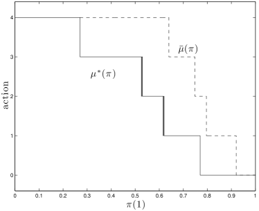
(a) Gaussian Observation Probabilities

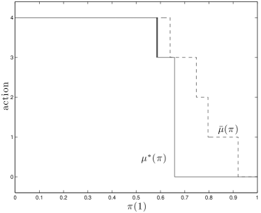
(b) Poisson Observation Probabilities

Figure 2: Optimal sampling strategy for action $u\in\{0\text{ (announce change)},1,2,3,4\}$ for a quickest-change detection problem with geometric change time. The parameters are specified in Example 2 and 3 in Sec.VI. The optimal strategy $\mu^{*}(\pi)$ is monotone decreasing in $\pi(1)$ and is upper bounded by myopic strategy $\bar{\mu}$ according to Theorem 5.

Example 3. Optimal Sampling Quickest Detection with Markov Modulated Poisson measurements: The parameters here are identical to Example 2 except that the observations are generated by a discrete time Markov Modulated Poisson process. That is, at each time $k$, observations are generated according to the Poisson distribution $B_{xy}=(\lambda_{x})^{y-1}\frac{e^{-\lambda_{x}}}{(y-1)!}$ where the rates $\lambda_{1}=1$, $\lambda_{2}=1.5$. Since (A3) holds for Poisson distribution, Theorem 2 applies. Fig.2(b) illustrates the optimal strategy. As in Example 2, the myopic strategy $\bar{\mu}(\pi)$ forms an upper bound.

Example 4. Optimal Sampling with Phase-Distributed Change Time: Here we consider optimal sampling quickest detection with PH-distributed change time. Consider a 3-state ($X=3$) Markov chain observed in noise with parameters $f=10$, $d=0.4$, $m(e_{i},u)=1$,

$$A=\begin{bmatrix}1&0&0\\ 0.7&0.3&0\\ 0.3&0.4&0.3\end{bmatrix},B=\begin{bmatrix}0.8&0.2&0\\ 0.1&0.8&0.1\\ 0&0.1&0.9\end{bmatrix},\{D_{1},D_{2},D_{3},D_{4}\}=\{1,2,4,5\}.$$

So $\Pi(X)$ is a 2-dimensional unit simplex. The optimal strategy was computed by forming a grid of 8000 values in the 2-dimensional unit simplex, and then solving the value iteration algorithm (38) over this grid on a horizon $N$ such that $\sup_{\pi}|V_{N}(\pi)-V_{N-1}(\pi)|<10^{-6}$. Fig.3(a) shows the optimal strategy.

It can be verified that the transition matrix $A$ satisfies (A3), (A6) and (A7) for $\alpha=100$. Also the observation distribution $B$ satisfies (A2). Therefore Theorem 5 holds and the optimal strategy is upper bounded by the myopic strategy $\bar{\mu}(\pi)$ defined in (31). Fig. 3(b) shows the myopic strategy $\bar{\mu}(\pi)$. As a bound for the optimal stopping region, we used the myopic stopping set $\underline{\mathcal{S}}$ defined in (30). In Fig.3(b) these are represented by ‘0’.

 

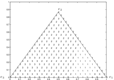
(a) Optimal Policy $\mu^{*}(\pi)$

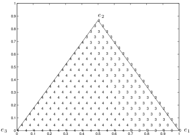
(b) Myopic Upper Bound $\bar{\mu}(\pi)$

Figure 3: Optimal sampling strategy for action $u\in\{0\text{ (announce change)},1,2,3,4\}$ for a quickest-change detection problem with PH-distributed time specified by 3-state Markov chain in Example 4 of Sec.VI. The belief space $\Pi(X)$ is a two dimensional unit simplex (equilateral triangle). The optimal strategy is upper bounded by myopic strategy $\bar{\mu}(\pi)$ according to Theorem 5.

VII Discussion

The paper presented structural results for the optimal sampling strategy of a Markov chain given noisy measurements. An example dealing with quickest change detection with optimal sampling was discussed to motivate the main results. Such problems are instances of partially observed Markov decision processes (POMDPs) and computing the optimal sampling strategy is intractable in general. However, this paper shows that under reasonable conditions on the sampling costs, transition matrix and noise distribution, one can say a lot about the optimal strategy and achievable cost using tools in stochastic dominance and lattice programming. There main results were: Theorems 1 and 2 gave sufficient conditions for the existence of a monotone optimal sampling strategy (with respect to the posterior distribution) when the underlying Markov chain had two states. It justified the intuition that one should make measurements less frequently when the underlying state is away from the target state. Theorem 4 and Theorem 5 gave sufficient conditions for the myopic sampling strategy to form a lower bound or upper bound to the optimal sampling strategy for multi-state Markov chains. Theorem 6 gave a partial ordering for the transition matrix and noise distributions so that the expected cost of the optimal sampling strategy decreased as these parameters increased. This yields useful information on the achievable optimal cost of an otherwise intractable problem. Theorem 7, gave explicit bounds on the sensitivity of the total sampling cost with respect to sampling strategy in terms of the Kullback Leibler divergence between the noise distributions. Theorem 9 gave several useful structural properties of the optimal Bayesian filtering update including sufficient conditions that preserve monotonicity of the filter with observation, prior distribution, transition matrix and noise distribution.

The assumptions (A1-A7) used in this paper are set valued; so even if the precise parameters (transition probabilities, observation distribution, costs) are not known, as long as they belong to the appropriate sets, the structural results hold. Thus the results have an inherent robustness.

Finally, it is interesting to note that the results derived in this paper on sampling control do not apply to general measurement control problems where the action affects the observation distribution rather than transition kernel. The reason is that it is not possible to find two non-trivial stochastic matrices (kernels) $B$ and $\bar{B}$ such that the belief updates satisfy (i) $T(\pi,y;B)\geq_{r}T(\pi,y;\bar{B})$ and normalization measure satisfies (ii) $\sigma(\pi,\cdot,B)\geq_{s}\sigma(\pi,\cdot;\bar{B})$. In [16], it is claimed that if $B$ TP2 dominates $\bar{B}$ then (i) and (ii) hold. However, we have found that the only examples of stochastic kernels that satisfy the TP2 dominance are the trivial example$B=\bar{B}$. In our paper, which deals with sampling control, the ordering (29) was constructed so that two transition matrices $A$ and $\bar{A}$ satisfy (i) and (ii) with $B,\bar{B}$ replaced by $A,\bar{A}$. This ordering was used in Assumption (A6).

-A Value Iteration Algorithm

The proof of the structural results in this paper will use the value iteration algorithm [7]. Let $n=1,2,\ldots,$ denote iteration number. The value iteration algorithm proceeds as follows:

$$V_{n+1}(\pi) =\min_{u\in\mathcal{U}}Q_{n}(\pi,u),\text{ where }Q_{n}(\pi,u)=C(\pi,u)+\sum_{y\in\mathbb{Y}}V_{n}\left(T(\pi,y,u)\right)\sigma(\pi,y,u),$$

and $$Q_{n}(\pi,0)=C(\pi,0)\text{ initialized by }V_{0}(\pi)=0.$$ (38)

Let $\mathcal{B}(X)$ denote the set of bounded real-valued functions on $\Pi(X)$. Then for any $V$ and $\tilde{V}\in\mathcal{B}(X)$, define the sup-norm metric $\sup\|V(\pi)-\tilde{V}(\pi)\|$, $\pi\in\Pi(X)$. Then $\mathcal{B}(X)$ is a Banach space. The value iteration algorithm (38) will generate a sequence of value functions $\{V_{k}\}\subset\mathcal{B}(X)$ that will converge uniformly (sup-norm metric) as $k\rightarrow\infty$ to $V(\pi)\in\mathcal{B}(X)$, the optimal value function of Bellman’s equation. However, since the belief state space $\Pi(X)$ is an uncountable set, the value iteration algorithm (38) do not translate into practical solution methodologies as $V_{k}(\pi)$ needs to be evaluated at each $\pi\in\Pi(X)$, an uncountable set. Nevertheless, the value iteration algorithm provides a natural method for proving our results on the structure of the optimal strategy via mathematical induction.

-B Proof of Theorem 1

To prove the existence of a monotone optimal strategy, we will show that $Q(\pi,u)$ in (17) is a submodular function on the poset $[\Pi(X),\geq_{r}]$. Note that $[\Pi(X),\geq_{r}]$ is a lattice since given any two belief states $\pi_{1},\pi_{2}\in\Pi(X)$, $\sup\{\pi:\pi\leq_{r}\pi_{1},\pi\leq_{r}\pi_{2}\}$ and $\inf\{\pi:\pi\geq_{r}\pi_{1},\pi\geq_{r}\pi_{2}\}$ lie in $\Pi(X)$. For $X=2$, $\Pi(X)$ is the unit interval [0,1] and in this case $[\Pi(X),\geq_{r}]$ is a chain (totally ordered set).

Definition 3 (Submodular function [25])

$f:\Pi(X)\times\{1,2\}\rightarrow\mathbb{R}$ is submodular (antitone differences) if $f(\pi,u)-f(\pi,\bar{u})\leq f(\tilde{\pi},u)-f(\tilde{\pi},\bar{u})$, for $\bar{u}\leq u$, $\pi\geq_{r}\tilde{\pi}$.

The following result says that for a submodular function $Q(\pi,u)$, $\mu^{*}(\pi)=\operatorname{argmin}_{u}Q(\pi,u)$ is increasing in its argument $\pi$. This will be used to prove the existence of a monotone optimal strategy in Theorem 1.

Theorem 10 ([25])

If $f:\Pi(X)\times\mathcal{U}\rightarrow\mathbb{R}$ is submodular, then there exists a $\mu^{*}(\pi)=\operatorname{argmin}_{u\in\mathcal{U}}f(\pi,u)$, that is MLR increasing on $\Pi(X)$, i.e., $\tilde{\pi}\geq_{r}{\pi}\implies\mu^{*}(\pi)\leq\mu^{*}(\tilde{\pi})$. ∎

Finally, we state the following result.

Theorem 11

The sequence of value function $\{V_{n}(\pi)$, $n=1,2,\ldots\}$, generated by the value iteration algorithm (38), and optimal value function $V(\pi)$ defined in (17) satisfy:
(i) $V_{n}(\pi)$ and $V(\pi)$ are concave in $\pi\in I$.
(ii) Under (A1), (A2), (A3), $V_{n}(\pi)$ and $V(\pi)$ are increasing in $\pi$ with respect to the MLR stochastic order on $\Pi(X)$. ∎

Statement (i) is well known for POMDPs, see [5] for a tutorial description. Statement (ii) is proved in [16, Proposition 1] using mathematical induction on the value iteration algorithm.

Proof: With the above preparation, we present the proof of Theorem 1.

The first claim follows from the general result that the stopping set $\mathcal{S}$ for a POMDP is always a convex subset of $\Pi(X)$ – see Theorem 4. Of course, a one dimensional convex set is an interval and since $e_{1}\in\mathcal{S}$, it follows that the interval $\mathcal{S}=(\pi_{1}^{*},1]$.

In light of the first claim, the optimal strategy is of the form

$$\mu^{*}(\pi)=\begin{cases}0&\pi\in\mathcal{S}\\ \operatorname{argmin}_{u\in\{1,2,\ldots,L\}}Q(\pi,u)&\pi\in\Pi(X)-\mathcal{S}\end{cases}$$

So to prove the second claim, we only need to focus on belief states in the interval $\Pi(X)-\mathcal{S}=[0,\pi_{1}^{*}]$ and consider actions $u\in\{1,2,\ldots,L\}$. To prove that $\mu^{*}(\pi)$ is MLR increasing in $\pi\in\Pi(X)-\mathcal{S}$, from Theorem 10 we need to prove that $Q(\pi,u)$ is submodular, that is

$$Q(\pi,u)-Q(\pi,\bar{u})-Q(\bar{\pi},u)+Q(\bar{\pi},\bar{u})\leq 0,\quad u>\bar{u},\;\pi\geq_{r}\bar{\pi}.$$

From (17), the left hand side of the above expression is

$$C(\pi,u)-C(\pi,\bar{u})-C({\bar{\pi}},\bar{u})+C({\bar{\pi}},\bar{u})$$

$$+ \sum_{y}V(T(\pi,y,u))\left[\sigma(\pi,y,u)-\sigma(\pi,y,\bar{u})-\sigma(\bar{\pi},y,u)+\sigma({\bar{\pi}},y,\bar{u})\right]$$

$$+ \sum_{y}\left[V(T(\pi,y,u))-V(T({\bar{\pi}},y,u))\right]\sigma(\pi,y,u)+\sum_{y}\left[V(T(\pi,y,u))-V(T(\pi,y,\bar{u}))\right]\sigma(\pi,y,\bar{u})$$

$$+ \sum_{y}\left[V(T(\bar{\pi},y,\bar{u}))-V(T(\pi,y,u))\right]\sigma(\bar{\pi},y,\bar{u})$$ (39)

Since the cost is submodular by (A4), the first line of (39) is negative. Since $V(\pi)$ is MLR increasing from Theorem 11 and $T(\pi,y,u)$ is MLR increasing in $y$ from Theorem 9(4), it follows that $V(T(\pi,y,u))$ is MLR increasing in $y$. Therefore, since $\sigma(\pi,\cdot,u)$ is submodular from Theorem 9(3), the second line of (39) is negative.

It only remains to prove that the third and fourth lines of (39) are negative. From statements (1) and (6) of Theorem 9, it follows that $T(\pi,y,u)\geq_{r}T(\pi,y,\bar{u})\geq_{r}T({\bar{\pi}},y,\bar{u})$ and $T(\pi,y,u)\geq_{r}T({\bar{\pi}},y,u)\geq_{r}T({\bar{\pi}},y,\bar{u})$. Now we use the assumption that $X=2$. So the belief state space $\Pi(X)$ is a one dimensional simplex that can be represented by $\pi(2)\in[0,1]$. So below we represent $\pi$, $T(\pi,y,u)$, etc. by their second elements. Therefore using concavity of $V(\cdot)$, we can express the last two summations in (39) as follows:

$$V(T(\pi,y,u))-V(T(\pi,y,\bar{u})) \leq\left[T(\pi,y,u)-T(\pi,y,\bar{u})\right]\frac{V(T(\pi,y,u))-V(T({\bar{\pi}},y,u))}{T(\pi,y,u)-T({\bar{\pi}},y,u)}$$

$$V(T({\bar{\pi}},y,\bar{u}))-V(T(\pi,y,u)) \leq\frac{T({\bar{\pi}},y,\bar{u})-T({\bar{\pi}},y,u)}{T(\pi,y,\bar{u})-T({\bar{\pi}},y,u)}\left[V(T(\pi,y,u))-V(T({\bar{\pi}},y,u))\right]$$

$$+V(T({\bar{\pi}},y,u))-V(T(\pi,y,u))$$

Using these expressions, the summation of the last two lines of (39) are upper bounded by

$$\sum_{y}\left[V(T(\pi,y,u))-V(T({\bar{\pi}},y,u))\right]\biggl{[}\sigma(\bar{\pi},y,u)+\frac{T(\pi,y,u)-T(\pi,y,\bar{u})}{T(\pi,y,u)-T({\bar{\pi}},y,u)}\sigma(\pi,y,\bar{u})\\ +\frac{T({\bar{\pi}},y,\bar{u})-T(\pi,y,u)}{T(\pi,y,u)-T({\bar{\pi}},y,u)}\sigma({\bar{\pi}},y,\bar{u})\biggr{]}$$ (40)

Since $V(\pi)$ is MLR increasing (Theorem 11) and $T(\pi,y,u)\geq_{r}T(\bar{\pi},y,u)$ (using the fact that $\pi\geq_{r}\bar{\pi}$ and Statement 1 of Theorem 9), clearly $V(T(\pi,y,u))-V(T({\bar{\pi}},y,u))\geq 0$. The term in square brackets in (40) can be expressed as (see [1])

$$\frac{B_{2y}B_{1y}(\pi-{\bar{\pi}})(A^{D_{2}}|_{22}-A^{D_{2}}|_{12}-A^{D_{1}}|_{22}-A^{D_{1}}|_{12})}{\sigma(\pi,y,u)[T(\pi,y,u)-T({\bar{\pi}},y,u)]}$$

By Assumption (A5)(ii) the above term is negative. Hence (39) is negative, thereby concluding the proof.

-C Proof of Theorem 3

Statement 1: Consider Bellman’s equation (17) and define $\underline{V}(\pi)=V(\pi)-\alpha C(\pi,L)$. It is easily checked that $\underline{V}(\pi)$ satisfies Bellman’s equation with costs $C(\pi,u)$ replaced by $\underline{C}(\pi,u)$ defined in (28). Also since the term being subtracted, namely, $\alpha C(\pi,L)$ is functionally independent of the minimization variable $u$, the argument of the minimum of (17), which is the optimal strategy $\mu^{*}(\pi)$, is unchanged.

Statement 2: Since our aim is to transform the delay cost to yield a MLR increasing submodular transformed cost, for notational convenience assume the measurement cost $m(x,u)=0$. From its definition in (28), straightforward computations yield that the transformed cost is

$$\underline{C}(\pi,0) ={f}^{\prime}\pi-\alpha de_{1}^{\prime}(I+A+\cdots A^{D_{L}-1})\pi$$

$$\underline{C}(\pi,u) =de_{1}^{\prime}\left((1-\alpha)I+\alpha A^{D_{L}}\right)^{\prime}(I+A+\cdots+A^{D_{u}-1})^{\prime}\pi,\quad u\in\{1,2,\ldots,L\}$$

So clearly for $\alpha\geq 0$, $\underline{C}(e_{1},0)\leq\underline{C}(e_{2},0)$, and so $\underline{C}(\pi,0)$ is MLR increasing.

We now give conditions for $\underline{C}(\pi,u)$, for $u\in\{1,2,\ldots,L\}$ to be MLR increasing in $\pi\in\Pi(X)$. By (A2), $(I+A+\cdots+A^{D_{u}-1})^{\prime}\pi$ is MLR increasing in $\pi\in\Pi(X)$. So for $\underline{C}(\pi,u)$ to be MLR increasing in $\pi$, it suffices to choose $\alpha$ so that the elements of $\left((1-\alpha)I+\alpha A^{D_{L}}\right)e_{1}$ are increasing. Given the structure of $A$ in (27), it follows that

$$\left((1-\alpha)I+\alpha A^{D_{L}}\right)e_{1}=\begin{bmatrix}1\\ \alpha(1-A_{22}^{D_{L}})\end{bmatrix}$$

So choosing $\alpha\geq 1/(1-A_{22}^{D_{L}})$ is sufficient for $\underline{C}(\pi,u)$ to be MLR increasing in $\pi$ for $u\in\{1,2,\ldots,L\}$ and therefore for $u\in\{0,1,\ldots,L\}$.

Next for the transformed cost $\underline{C}(\pi,u)$ to be submodular for $u\in\{1,2,\ldots,L\}$, we require $\underline{C}(\pi,u+1)-\underline{C}(\pi,u)$ to be MLR decreasing in $\pi$. Straightforward computations yield for $u\in\{1,2,\ldots,L\}$,

$$\underline{C}(\pi,u+1)-\underline{C}(\pi,u)=de_{1}^{\prime}\left((1-\alpha)I+\alpha A^{D_{L}}\right)^{\prime}(A^{D_{u}}+A^{D_{u}+1}+\cdots+A^{D_{u+1}})^{\prime}\pi$$

So for $\underline{C}(\pi,u)$ to be submodular, it suffices to choose $\alpha$ so that the elements of $\left((1-\alpha)I+\alpha A^{D_{L}}\right)e_{1}$ are decreasing, i.e., $\alpha\leq 1/(1-A_{22}^{D_{L}})$.

Therefore choosing $\alpha=1/(1-A_{22}^{D_{L}})$ is sufficient for the transformed cost $\underline{C}(\pi,u)$ to be both MLR increasing for $u\in\{0,1,\ldots,L\}$ and submodular for $u\in\{1,2,\ldots,L\}$ on the poset $[\Pi(X)-\mathcal{S},\geq_{r}]$.

-D Proof of Theorem 4

Statement 1: The proof of convexity of the stopping set $\mathcal{S}$ follows from arguments in [15]. We repeat this for completeness here. Pick any two belief states $\pi_{1},\pi_{2}\in\mathcal{S}$. To demonstrate convexity of $\mathcal{S}$, we need to show for any $\lambda\in[0,1]$, $\lambda\pi_{1}+(1-\lambda)\pi_{2}\in\mathcal{S}$. Since $V(\pi)$ is concave (by Theorem 11 above), it follows from (17) that

$$V(\lambda\pi_{1}+(1-\lambda)\pi_{2}) \geq\lambda V(\pi_{1})+(1-\lambda)V(\pi_{2})$$

$$=\lambda Q(\pi_{1},0)+(1-\lambda)Q(\pi_{2},0)\text{ (since $\pi_{1},\pi_{2}\in\mathcal{S}$) }$$

$$=Q(\lambda\pi_{1}+(1-\lambda)\pi_{2},0)\text{ (since $Q_{1}(\pi,0)$ is linear in $\pi$) }$$

$$\geq V(\lambda\pi_{1}+(1-\lambda)\pi_{2})\text{ (since $V(\pi)$ is the optimal value function) }$$ (41)

Thus all the inequalities above are equalities, and $\lambda\pi_{1}+(1-\lambda)\pi_{2}\in\mathcal{S}$.

Statement 2: Since the costs $C(\pi,u)$ are non-negative, so is $V(\pi)$ in (17). So from (17)., $C(\pi,0)\leq C(\pi,u)\implies Q(\pi,0)\leq Q(\pi,u)\implies\pi\in\mathcal{S}$. Therefore $\underline{\mathcal{S}}\subset\mathcal{S}$.

Statement 3: The proof is similar to [16, Proposition 2] with the important difference that in [16] the TP2 ordering of transition matrices is used instead of (A6). However, the TP2 ordering (see [16] for definition) does not yield any non-trivial example.

Since $D_{u}<D_{u+1}$, (A6) implies $A^{D_{u}}\succeq A^{D_{u+1}}$. So by Statement 6(a) of Theorem 9, for $u>\bar{u}$, $T(\pi,y,u)\leq_{r}T(\pi,y,\bar{u})$. By Theorem 11, $V(\pi)$ is MLR increasing in $\pi$. Therefore $V(T(\pi,y,u))\leq V(T(\pi,y,\bar{u}))$. So

$$\sum_{y}V(T(\pi,y,u)\sigma(\pi,y,u)\leq\sum_{y}V(T(\pi,y,\bar{u})\sigma(\pi,y,u),\quad u>\bar{u}.$$

Since $T(\pi,y,\bar{u})$ is MLR increasing in $y$ (Statement 4 of Theorem 9) and $V(\pi)$ is MLR increasing in $\pi$, clearly $V(T(\pi,y,\bar{u}))$ is increasing in $y$. Also (A6) implies $A^{D_{u}}\succeq A^{D_{u+1}}$ and so $\sigma(\pi,\cdot,u)\leq_{s}\sigma(\pi,\cdot,\bar{u})$ from Statement 6(b) of Theorem 9. So

$$\sum_{y}V(T(\pi,y,\bar{u})\,\sigma(\pi,y,u)\leq\sum_{y}V(T(\pi,y,\bar{u})\,\sigma(\pi,y,\bar{u}),\quad u>\bar{u}.$$

Therefore, $\sum_{y}V(T(\pi,y,u)\sigma(\pi,y,u)\leq\sum_{y}V(T(\pi,y,\bar{u})\sigma(\pi,y,\bar{u})$ which is equivalent to $Q(\pi,u)-Q(\pi,\bar{u})\leq C(\pi,u)-C(\pi,\bar{u})$. Then [16, Lemma 2.2] implies that the minimizers of $Q(\pi,u)-Q(\pi,\bar{u})$ are larger than that of $C(\pi,u)-C(\pi,\bar{u})$. That is $\mu^{*}(\pi)\geq\bar{\mu}(\pi)$ for $\pi\in\Pi(X)$.

Statement 4: By (A4), $C(\pi,u)$ is submodular on the poset $[\Pi(X),\geq_{r}]$. So using Theorem 10 it follows that $\underline{\mu}(\pi)$ is MLR increasing.

-E Proof of Theorem 5

Statements 1 and 2 follows directly from Theorem 4.

Statement 3: We prove this in the following steps.

Step 1. $\mu^{*}(\pi)$ remains invariant with transformed cost: For costs $\bar{C}(\pi,u)$ Bellman’s equation yields the same optimal strategy $\mu^{*}(\pi)$ as costs $C(\pi,u)$. To see this, consider Bellman’s equation (17) and define $\bar{V}(\pi)=V(\pi)+\alpha de_{1}^{\prime}A^{\prime}\pi$. It is easily checked that $\bar{V}(\pi)$ satisfies Bellman’s equation with costs $C(\pi,u)$ replaced by $\bar{C}(\pi,u)$ defined in (28). Also since the term being added, namely $\alpha de_{1}^{\prime}A^{\prime}\pi$ is functionally independent of the minimization variable $u$, the argument of the minimum of (17), which is the optimal strategy $\mu^{*}(\pi)$, is unchanged.

Step 2. $\bar{C}(\pi,u)$ is MLR decreasing: We show that (A7) implies that $\bar{C}(\pi,u)$ is MLR decreasing, i.e., $-\bar{C}(\pi,u)$ is MLR increasing and satisfies (A1).

First consider $\bar{C}(\pi,0)$. Note $\bar{C}(e_{1},0)=\alpha d$, and $\bar{C}(e_{i},0)=f+\alpha A_{i1}$ for $i>1$. So $\bar{C}(e_{1},0)\geq\bar{C}(e_{2},0)$ if $\alpha>f/(d(1-A_{21}))$. Since $\alpha>0$ and $A$ is TP2 (Assumption A3), $A_{i1}>A_{i+1,1}$. So clearly $\bar{C}(e_{i},0)\geq\bar{C}(e_{i+1},0)$ for $i\geq 2$.

Next consider $\bar{C}(\pi,u)$, $u\in\{1,2,\ldots,L\}$. Note $\bar{C}(e_{1},u)=dD_{u}$ and

$$\bar{C}(e_{i},u)=d(A_{i1}+A^{2}|_{i1}+\cdots+A^{D_{u}-1}|_{i1})+\alpha d(A_{21}-A^{D_{u}+1}|_{21}).$$ (42)

Clearly $\bar{C}(e_{i},u)<d(D_{u}-1)+\alpha d(A_{i1}-A^{D_{u}+1}|_{i1})$. Also $A_{i1}-A^{D_{u}+1}|_{i1}\leq 0$ since $A^{D_{u}+1}|_{i1}=A_{i1}+\sum_{j>1}A_{ij}A^{D_{u}}|_{j1}$. Therefore for non-negative $\alpha$, $\bar{C}(e_{1},u)\geq\bar{C}(e_{i},u)$, $i\geq 2$. Also for $\bar{C}(e_{i},u)\geq\bar{C}(e_{i+1},u)$, $i\geq 2$, clearly from (42) it follows that (A7)(ii) is sufficient.

Step 3: $\bar{C}(\pi,u)$, $u\geq 1$, is submodular (satisfies (A4)). This follows similar to Step 2.

Step 4: With the above three steps, we can now apply Theorem 4, except that $\bar{C}(\pi,u)$ is MLR decreasing instead of MLR increasing as required by (A1). By a very similar proof to Theorem 4, it follows that $\bar{\mu}(\pi)\geq\mu^{*}(\pi)$.

Statement 4: Follows trivially from Statement 3 for the $X=2$ case.

-F Proof of Theorem 6

Part 1: We first prove that dominance of transition matrices $A\succeq\bar{A}$ (with respect to (29)) results in dominance of optimal costs, i.e., $V(\pi;A)\geq V(\pi;\bar{A})$. The proof is by induction. $V_{0}(\pi;A)\geq V_{0}(\pi;\bar{A})=0$ by the initialization of the value iteration algorithm (38). Next, to prove the inductive step assume that $V_{n}(\pi;A)\geq V_{n}(\pi;\bar{A})$ for $\pi\in\Pi(X)$. By Theorem 11(ii), under (A1), (A2), (A3), $V_{n}(\pi;A)$ and $V_{n}(\pi;\bar{A})$ are MLR increasing in $\pi\in\Pi(X)$. From Statement 6(a) of Theorem 9, it follows that $T(\pi,y,u;A)\geq_{r}T(\pi,y,u;\bar{A})$. This implies

$$V_{n}(T(\pi,y,u;A);A)\geq V_{n}(T(\pi,y,u;\bar{A});A),\quad A\succeq\bar{A}.$$

Since $V_{n}(\pi;A)\geq V_{n}(\pi;\bar{A})\;\forall\pi\in\Pi(X)$ by assumption, clearly $V_{n}(T(\pi,y,u,\bar{A});A)\geq V_{n}(T(\pi,y,u,\bar{A});\bar{A})$. Therefore

$$V_{n}(T(\pi,y,u;A);A)\geq V_{n}(T(\pi,y,u;\bar{A});A)\geq V_{n}(T(\pi,y,u,\bar{A});\bar{A}),\quad A\succeq\bar{A}.$$

Under (A2), (A3), Statement 4 of Theorem 9 says that $T(\pi,y,u;A);A)$ is MLR increasing in $y$. Therefore, $V_{n}(T(\pi,y,u;A);A)$ is increasing in $y$. Also from Statement 2 of Theorem 9, $\sigma(\pi,\cdot,u;A)\geq_{s}\sigma((\pi,\cdot,u;\bar{A})$ for $A\succeq\bar{A}$. Therefore,

$$\sum_{y}V_{n}(T(\pi,y,u;A);A)\sigma(\pi,\cdot,u;A)\geq\sum_{y}V_{n}(T(\pi,y,u;\bar{A});\bar{A})\sigma(\pi,\cdot,u;\bar{A}).$$ (43)

Next, we claim that under (A1) and (A2), $A\succeq\bar{A}$ implies that $C(\pi,u;A)\geq C(\pi,u,;\bar{A})$. This follows since $c(e_{i},u)$ defined in (15) has increasing components by (A1) and $({A^{l}})^{\prime}\pi\geq_{r}({\bar{A}}^{l})^{\prime}\pi$ (Statement 5(b), Theorem 9). Therefore, $c_{u}^{\prime}({A^{l}})^{\prime}\pi\geq c_{u}^{\prime}({\bar{A}}^{l})^{\prime}\pi$ implying that $C(\pi,u;A)\geq C(\pi,u,\bar{A})$. This together with (43) implies

$$C(\pi,u;A)+\sum_{y}V_{n}(T(\pi,y,u;A);A)\sigma(\pi,\cdot,u;A)\geq C(\pi,u,\bar{A})+\sum_{y}V_{n}(T(\pi,y,u;\bar{A});\bar{A})\sigma(\pi,\cdot,u;\bar{A})$$

Minimizing both sides with respect to action $u$ yields $V_{n+1}(\pi;A)\geq V_{n+1}(\pi;\bar{A})$ and concludes the induction argument.

Part 2: Next we show that dominance of observation distributions $B\succeq_{B}\bar{B}$ (with respect to the order (32)) results in dominance of the optimal costs, namely $V(\pi;B)\geq V(\pi,\bar{B})$. Let $T(\pi,y,u)$ and $\bar{T}(\pi,y,u)$ denote the Bayesian filter update with observation $B$ and $\bar{B}$, respectively, and let $\sigma(\pi,y,u)$ and $\bar{\sigma}(\pi,y,u)$ denote the corresponding normalization measures.

Then for $a\in\mathbb{Y}$,

$$T(\pi,a,u)=\sum_{y\in\mathbb{Y}}\bar{T}(\pi,y,u)\frac{\bar{\sigma}(\pi,y,u)}{\sigma(\pi,a,u)}P(a|y)\quad\text{ and }\sigma(\pi,a,u)=\sum_{y\in\mathbb{Y}}\bar{\sigma}(\pi,y,u)P(a|y).$$

Therefore, $\frac{\bar{\sigma}(\pi,y,u)}{\sigma(\pi,y,a)}P(a|y)$ is a probability measure wrt $y$. Since from Theorem 11, $V_{n}(\cdot)$ is concave for $\pi\in\Pi(X)$, using Jensen’s inequality it follows that

$$V_{n}(T(\pi,a,u);\bar{B}) =V_{n}\left(\sum_{y\in\mathbb{Y}}\bar{T}(\pi,y,u)\frac{\bar{\sigma}(\pi,y,u)}{\sigma(\pi,a,u)}P(a|y);\bar{B}\right)\geq\sum_{y\in\mathbb{Y}}V_{n}(\bar{T}(\pi,y,u);\bar{B})\frac{\bar{\sigma}(\pi,y,u)}{\sigma(\pi,a,u)}P(a|y)$$

implying $$\sum_{a}V_{n}(T(\pi,a,u);\bar{B})\sigma(\pi,a,u)\geq\sum_{y}V_{n}(\bar{T}(\pi,y,u);\bar{B})\bar{\sigma}(\pi,y,u).$$ (44)

With the above inequality, the proof of the theorem follows by mathematical induction using the value iteration algorithm (38). Assume $V_{n}(\pi;B)\geq V_{n}(\pi;\bar{B})$ for $\pi\in\Pi(X)$. Then

$$C(\pi,u)+\sum_{a}V_{n}(T(\pi,a,u);B)\sigma(\pi,a,u) \geq C(\pi,u)+\sum_{a}V_{n}(T(\pi,a,u);\bar{B})\sigma(\pi,a,u)$$

$$\geq C(\pi,u)+\sum_{y}V_{n}(\bar{T}(\pi,y,u);\bar{B})\bar{\sigma}(\pi,y,u)$$

where the second inequality follows from (44). Thus $V_{n+1}(\pi;B)\geq V_{n+1}(\pi;\bar{B})$. This completes the induction step. Since value iteration algorithm (38) converges uniformly, $V(\pi;B)\geq V(\pi;\bar{B})$ thus proving the theorem.

-G Proof of Theorem 7

Define the set of belief states $\bar{\mathcal{S}}=\cap_{u}\{\pi:(C_{u}-C_{0})^{\prime}\pi\geq 0\}$. Clearly $\bar{\mathcal{S}}\subseteq\mathcal{S}$. Let us characterize the set of observations such that the Bayesian filter update $T(\pi,y,u;\theta)$ lies in $\bar{\mathcal{S}}$ for any action $u$. Accordingly, define

$$\mathcal{R}_{\pi;\theta}=\{y:(C_{\bar{u}}-C_{0})^{\prime}T(\pi,y,u;\theta)\geq 0,\;\forall u,\bar{u}\in\{1,2,\ldots,L\}\},\quad y_{\pi;\theta}^{*}=\inf\{y:y\in\mathcal{R}^{c}_{\pi;\theta}\}.$$ (45)

Here $\mathcal{R}^{c}_{\pi;\theta}$ denotes the complement of set $\mathcal{R}_{\pi;\theta}$.

Lemma 1

Under (A2),(A3),(A4), the following hold for $\mathcal{R}_{\pi;\theta}$ and $y_{\pi;\theta}^{*}$ defined in (45):
(i) $\mathcal{R}^{c}_{\pi;\theta}=\{y:y\geq y_{\pi;\theta}^{*}\}$. (ii) $\pi\geq_{r}{\bar{\pi}}\implies\mathcal{R}_{\pi;\theta}\subset\mathcal{R}_{{\bar{\pi}};\theta}$. (iii) $\pi\geq_{r}{\bar{\pi}}\implies y_{\pi;\theta}^{*}<y_{{\bar{\pi}};\theta}^{*}$.

Proof:

The first assertion says that the set of observations for continuing is the set $\{y:y\geq y_{\pi;\theta}^{*}\}$. By (A4), $C_{\bar{u}}-C_{0}$ has decreasing elements. Since $T(\pi,y,u;\theta)$ is MLR increasing in $y$, clearly $(C_{\bar{u}}-C_{0})^{\prime}T(\pi,y,u;\theta)$ is decreasing in $y$. Therefore, there exists a $y_{\pi;\theta}^{*}$ such that $y\geq y_{\pi;\theta}^{*}$ implies $T(\pi,y,u;\theta)\in\mathcal{R}^{c}_{\pi;\theta}$. This proves the first statement. By (A4), $C_{\bar{u}}-C_{0}$ has decreasing elements. By (A2), (A3), $T(\pi,y,u;\theta)$ is MLR increasing in $\pi$. Therefore $(C_{\bar{u}}-C_{0})^{\prime}T(\pi,y,u;\theta)\geq(C_{\bar{u}}-C_{0})^{\prime}T(e_{X},y,u;\theta)$ which implies $\mathcal{R}_{\pi;\theta}\subset\mathcal{R}_{{\bar{\pi}};\theta}$. Statement (i) says that $T(\pi,y,u;\theta)$ is MLR increasing in $y$; statement (ii) says that $\mathcal{R}_{\pi;\theta}\subset\mathcal{R}_{{\bar{\pi}};\theta}$. Combining these yields $y_{\pi;\theta}^{*}\leq y_{{\bar{\pi}};\theta}^{*}$. ∎

For notational convenience denote the optimal strategy $\mu^{*}(\theta)$ as $\mu$. From (15), the total cost incurred by applying strategy $\mu(\pi)$ to model $\theta$ satisfies at time $n$

$$J_{\mu}^{(n)}(\pi;\theta) =C_{\mu(\pi)}^{\prime}\pi+\sum_{y\in\mathbb{Y}}J_{\mu}^{(n-1)}(T(\pi,y,\mu(\pi);\theta)\sigma(\pi,y,\mu(\pi);\theta)$$

$$=C_{\mu(\pi)}^{\prime}\pi+\sum_{y\in\mathcal{R}^{c}_{\pi;\theta}}J_{\mu}^{(n-1)}(T(\pi,y,\mu(\pi);\theta)\sigma(\pi,y,\mu(\pi);\theta)$$

since for $y\in\mathcal{R}_{\pi;\theta}$, $T(\pi,y,\mu(\pi);\theta)\in\bar{\mathcal{S}}$ and so $V(T(\pi,y,\mu(\pi);\theta))=0$.

Therefore, the absolute difference in total costs for models $\theta,\bar{\theta}$ satisfies

$$|J_{\mu}^{(n)}(\pi;\theta)-J_{\mu}^{(n)}(\pi;\bar{\theta})|\leq \sum_{y\in\mathcal{R}^{c}_{\pi;\theta}\cup\mathcal{R}^{c}_{\pi;\bar{\theta}}}|J_{\mu}^{(n-1)}(T(\pi,y,\mu(\pi);\theta)-J_{\mu}^{(n-1)}(T(\pi,y,\mu(\pi);\bar{\theta})|\,\sigma(\pi,y,\mu(\pi);\theta)$$

$$\quad+\sum_{y\in\mathcal{R}^{c}_{\pi;\theta}\cup\mathcal{R}^{c}_{\pi;\bar{\theta}}}J_{\mu}^{(n-1)}(T(\pi,y,\mu(\pi);\bar{\theta})\,\bigl{|}\sigma(\pi,y,\mu(\pi);\theta)-\sigma(\pi,y,\mu(\pi);\bar{\theta})\bigr{|}$$

$$\leq \sup_{\pi\in\Pi(X)}|J_{\mu}^{(n-1)}(\pi;\theta)-J_{\mu}^{(n-1)}(\pi;\bar{\theta})|\,\sum_{y\in\mathcal{R}^{c}_{\pi;\theta}\cup\mathcal{R}^{c}_{\pi;\bar{\theta}}}\sigma(\pi,y,\mu(\pi);\theta)$$

$$+\sup_{\pi\in\Pi(X)}J_{\mu}^{(n-1)}(\pi;\bar{\theta})\sum_{y\in\mathbb{Y}}\bigl{|}\sigma(\pi,y,\mu(\pi);\theta)-\sigma(\pi,y,\mu(\pi);\bar{\theta})\bigr{|}$$ (46)

We will upper bound the various terms on the RHS of (46). Statement (i) of Lemma 1 yields $\mathcal{R}^{c}_{\pi;\theta}\cup\mathcal{R}^{c}_{\pi;\bar{\theta}}=\{y\geq y_{\pi;\theta,\bar{\theta}}^{*}\}$ where $y_{\pi;\theta,\bar{\theta}}^{*}=\min(y_{\pi;\theta}^{*},y_{\pi;\bar{\theta}}^{*})$. Next Statement (iii) of Lemma 1 yields $y_{e_{X};\theta,\bar{\theta}}^{*}\leq y_{\pi;\theta,\bar{\theta}}^{*}$. Therefore,

$$\sup_{\pi\in\Pi(X)}|J_{\mu}^{(n-1)}(\pi;\theta)-J_{\mu}^{(n-1)}(\pi;\bar{\theta})| \,\sum_{y\in\mathcal{R}^{c}_{\pi;\theta}\cup\mathcal{R}^{c}_{\pi;\bar{\theta}}}\sigma(\pi,y,\mu(\pi);\theta)$$

$$\leq \sup_{\pi\in\Pi(X)}|J_{\mu}^{(n-1)}(\pi;\theta)-J_{\mu}^{(n-1)}(\pi;\bar{\theta})|\,\max_{u}\sum_{y\geq y_{e_{X};\theta,\bar{\theta}}^{*}}\sigma(\pi,y,u;\theta)$$

$$\leq \sup_{\pi\in\Pi(X)}|J_{\mu}^{(n-1)}(\pi;\theta)-J_{\mu}^{(n-1)}(\pi;\bar{\theta})|\,\max_{u}\sum_{y\geq y_{e_{X};\theta,\bar{\theta}}^{*}}\sigma(e_{X},y,u;\theta)$$

where the last line follows since $e_{X}\geq_{s}\pi$, and so Statement 2 of Theorem 9 implies $\sigma(\pi,\cdot,u;\theta)\leq_{s}\sigma(e_{X},\cdot,u;\theta)$. Also evaluating $\sigma(\pi,y,\mu(\pi);\theta)=\mathbf{1}_{X}^{\prime}B_{y}({A^{\prime}})^{\mu(\pi)}\pi$ defined in (10) yields

$$\sum_{y\in\mathbb{Y}}\bigl{|}\sigma(\pi,y,\mu(\pi);\theta)-\sigma(\pi,y,\mu(\pi);\bar{\theta})\bigr{|}\leq\max_{u}\sum_{y}\sum_{i}\sum_{j}|B_{jy}A^{u}|_{ij}-\bar{B}_{jy}\bar{A}^{u}|_{ij}|\pi(i)\\ \leq\max_{u}\max_{i}\sum_{y}\sum_{j}|B_{jy}A^{u}|_{ij}-\bar{B}_{jy}\bar{A}^{u}|_{ij}|$$ (47)

Finally, $\sup_{\pi\in\Pi(X)}J_{\mu}^{(n-1)}(\pi;\bar{\theta})\leq\max_{i\in\mathbb{X}}C(e_{i},0)$. Using these bound in (46) yields

$$\sup_{\pi\in\Pi(X)}|J_{\mu}^{(n)}(\pi;\theta)-J_{\mu}^{(n)}(\pi;\bar{\theta})|\leq\rho\,\sup_{\pi\in\Pi(X)}|J_{\mu}^{(n-1)}(\pi;\theta)-J_{\mu}^{(n-1)}(\pi;\bar{\theta})|+\max_{i\in\mathbb{X}}C(e_{i},0)\|\theta-\bar{\theta}\|$$ (48)

where $\rho_{\theta,\bar{\theta}}=\max_{u}\sum_{y\geq y_{e_{X};\theta,\bar{\theta}}^{*}}\sigma(e_{X},y,u;\theta)$ and $\|\theta-\bar{\theta}\|$ is given by (47). Since $\max_{u}\sum_{y\in\mathbb{Y}}\sigma(e_{X},y,u;\theta)=1$, then (A7) implies $\rho_{\theta,\bar{\theta}}=\max_{u}\sum_{y\geq y_{e_{X};\theta,\bar{\theta}}^{*}}\sigma(e_{X},y,u;\theta)<1$. Then starting with $J_{\mu}^{(0)}(\pi;\theta)=J_{\mu}^{(0)}(\pi;\bar{\theta})=0$, unravelling (48) yields (35).

Proof of Corollary 1: When $\theta$ and $\bar{\theta}$ have identical transition matrices, then (47) becomes

$$\max_{u}\max_{i}\sum_{j}A^{u}|_{ij}\sum_{y}|B_{jy}-\bar{B}_{jy}|$$

From Pinsker’s inequality [6], the total variation norm is bounded by Kullback-Leibler distance $D$ defined in (36) as

$$\sum_{y}|B_{jy}-\bar{B}_{jy}|\leq\sqrt{2\,D(B_{j}\|\bar{B}_{j})}$$

-H Proof of Theorem 9

We quote the following result from [8], which adapted to our notation reads

Theorem 12 ([8, Lemma 8.2, pp.382])

(i) Suppose $p(\cdot)$ and $q(\cdot)$ are integrable functions on $\mathbb{Y}$ and $f(\cdot)$ is increasing and non-negative. Then $\sum_{Y}f(y)p(y)\leq\sum_{Y}f(y)q(y)$ iff $\sum_{y\geq\bar{y}}p(y)\geq\sum_{y\geq\bar{y}}q(y)$.
(ii) Suppose $f_{i}$ is increasing for $i\in X$ and non-negative. Then for arbitrary vectors $p,q\in\mathbb{R}^{X}$, $f^{\prime}p\geq f^{\prime}q\text{ iff }\sum_{j\geq\bar{j}}p_{j}\geq\sum_{j\geq\bar{j}}q_{j}\text{ for all }\bar{j}\in\mathbb{X}$ ∎

The above theorem is similar to Statement (ii) of Theorem 8 with some important difference. Unlike Theorem 8, $p$ and $q$ need not be probability measures. On the other hand, Theorem 8 does not require $f$ to be non-negative.

Proof of Theorem 9: Statements 1, 2 and 4 of the theorem are proved in [16].

Statement 3: Suppose $\pi\geq_{r}{\bar{\pi}}$. Then clearly (A5)-(i) implies that

$$\sum_{j\geq q}\sum_{i}\left(A^{D_{u+1}}|_{ij}-A^{D_{u}}|_{ij}\right)\pi(i)\leq\sum_{j\geq q}\sum_{i}\left(A^{D_{u+1}}|_{ij}-A^{D_{u}}|_{ij}\right){\bar{\pi}}(i).$$

Also (A3) implies that $\sum_{y\geq q}B_{jy}$ is increasing in $j$. Then applying Theorem 12(i) yields

$$\sum_{j}\sum_{y\geq q}B_{jy}\sum_{i}\left(A^{D_{u+1}}|_{ij}-A^{D_{u}}|_{ij}\right)\pi(i)\leq\sum_{j}\sum_{y\geq q}B_{jy}\sum_{i}\left(A^{D_{u+1}}|_{ij}-A^{D_{u}}|_{ij}\right){\bar{\pi}}(i).$$

Statement 5(a): The proof is as follows: By definition ${A}^{\prime}\pi\geq_{r}{\bar{A}}^{\prime}\pi$ is equivalent to

$$\sum_{i\in\mathbb{X}}\sum_{m\in\mathbb{X}}\left(A_{ij}\bar{A}_{m,j+1}-\bar{A}_{ij}A_{m,j+1}\right)\pi_{i}\pi_{m}\leq 0.$$

Thus clearly (29) is a sufficient condition for ${A}^{\prime}\pi\geq_{r}{\bar{A}}^{\prime}\pi$.

Statement 5(b): Since $A\succeq\bar{A}$ implies $A^{\prime}\pi\geq_{r}\bar{A}^{\prime}\pi$ it follows from (A2) that $A^{\prime}A^{\prime}\pi\geq_{r}A^{\prime}\bar{A}^{\prime}\pi$. Also Statement 4(a) implies $A^{\prime}\bar{A}^{\prime}\pi\geq_{r}\bar{A}^{\prime}\bar{A}^{\prime}\pi$. Since the MLR order is transitive, these inequalities imply $A^{\prime}A^{\prime}\pi\geq_{r}\bar{A}^{\prime}\bar{A}^{\prime}\pi$. Continuing similarly, it follows that for any positive integer $l$, $({A^{l}})^{\prime}\pi\geq_{r}({\bar{A}}^{l})^{\prime}\pi$ .

Statement 6(a): This follows trivially since Bayes’ rule preserves MLR dominance. That is $\pi\geq_{r}{\bar{\pi}}$ implies $\frac{B_{y}\pi}{\mathbf{1}_{X}^{\prime}B_{y}\pi}\geq_{r}\frac{B_{y}{\bar{\pi}}}{\mathbf{1}_{X}^{\prime}B_{y}{\bar{\pi}}}$. Since by Statement 4(a), $A\succeq\bar{A}$ implies $A^{\prime}\pi\geq_{r}\bar{A}^{\prime}\pi$, applying the Bayes rule preservation of MLR dominance proves the result.

Statement 6(b): (iii) Since $A\succeq\bar{A}$ implies $A^{\prime}\pi\geq_{r}\bar{A}^{\prime}\pi$, it follows that $A^{\prime}\pi\geq_{s}\bar{A}^{\prime}\pi$. Next (A3) implies that $\sum_{y\geq q}B_{iy}$ is increasing in $i$. Therefore $\sum_{i\in\mathbb{X}}\sum_{y\geq q}B_{iy}[A^{\prime}\pi](i)\geq\sum_{i\in\mathbb{X}}\sum_{y\geq q}B_{iy}[\bar{A}^{\prime}\pi](i)$.

References

• [1] S.C. Albright. Structural results for partially observed markov decision processes. Operations Research, 27(5):1041โ€“1053, Sept.-Oct. 1979.
• [2] S.ย Athey. Monotone comparative statics under uncertainty. The Quarterly Journal of Economics, 117(1):187โ€“223, 2002.
• [3] T.ย Banerjee and V.ย Veeravalli. Data-efficient quickest change detection with on-off observation control. Sequential Analysis, 31:40โ€“77, 2012.
• [4] D.P. Bertsekas. Dynamic Programming and Optimal Control, volume 1 and 2. Athena Scientific, Belmont, Massachusetts, 2000.
• [5] A.ย R. Cassandra. Exact and Approximate Algorithms for Partially Observed Markov Decision Process. PhD thesis, Brown University, 1998.
• [6] T.M. Cover and J.A. Thomas. Elements of Information Theory. Wiley-Interscience, 2006.
• [7] O.ย Hernรกndez-Lerma and J.ย Bernard Laserre. Discrete-Time Markov Control Processes: Basic Optimality Criteria. Springer-Verlag, New York, 1996.
• [8] D.P. Heyman and M.J. Sobel. Stochastic Models in Operations Research, volumeย 2. McGraw-Hill, 1984.
• [9] S.ย Karlin and Y.ย Rinott. Classes of orderings of measures and related correlation inequalities. I. Multivariate totally positive distributions. Journal of Multivariate Analysis, 10:467โ€“498, 1980.
• [10] V.ย Krishnamurthy. Algorithms for optimal scheduling and management of hidden Markov model sensors. IEEE Trans.ย Signal Proc., 50(6):1382โ€“1397, June 2002.
• [11] V.ย Krishnamurthy. Bayesian sequential detection with phase-distributed change time and nonlinear penalty โ€“ a lattice programming pomdp approach. IEEE Transactions on Information Theory, 57(3), Oct. 2011. http://arxiv.org/abs/1011.5298.
• [12] V.ย Krishnamurthy. Quickest detection with social learning: How local and global decision makers interact. IEEE Transactions on Information Theory, 58, 2012. http://arxiv.org/abs/1007.0571.
• [13] V.ย Krishnamurthy, R.ย Bitmead, M.ย Gevers, and E.ย Miehling. Sequential detection with mutual information stopping cost: Application in GMTI radar. IEEE Trans.ย Signal Proc., 60(2):700โ€“714, 2012.
• [14] V.ย Krishnamurthy and D.ย Djonin. Structured threshold policies for dynamic sensor schedulingโ€“a partially observed Markov decision process approach. IEEE Trans.ย Signal Proc., 55(10):4938โ€“4957, Oct. 2007.
• [15] W.S. Lovejoy. On the convexity of policy regions in partially observed systems. Operations Research, 35(4):619โ€“621, July-August 1987.
• [16] W.S. Lovejoy. Some monotonicity results for partially observed Markov decision processes. Operations Research, 35(5):736โ€“743, Sept.-Oct. 1987.
• [17] A.ย Muller and D.ย Stoyan. Comparison Methods for Stochastic Models and Risk. Wiley, 2002.
• [18] M.F. Neuts. Structured stochastic matrices of M/G/1 type and their applications. Marcel Dekker, N.Y., 1989.
• [19] C.ย H. Papadimitrou and J.N. Tsitsiklis. The compexity of Markov decision processes. Mathematics of Operations Research, 12(3):441โ€“450, 1987.
• [20] H.ย V. Poor and O.ย Hadjiliadis. Quickest Detection. Cambridge, 2008.
• [21] U.ย Rieder. Structural results for partially observed control models. Methods and Models of Operations Research, 35:473โ€“490, 1991.
• [22] ANย Shiryaev. On optimum methods in quickest detection problems. Theory of Probability and its Applications, 8:22, 1963.
• [23] A.N. Shiryayev. Optimal stopping rules. Springer-Verlag, 1978.
• [24] A.G. Tartakovsky and V.V. Veeravalli. General asymptotic Bayesian theory of quickest change detection. Theory of Probability and its Applications, 49(3):458โ€“497, 2005.
• [25] D.M. Topkis. Supermodularity and Complementarity. Princeton University Press, 1998.
• [26] W.ย Whitt. Multivariate monotone likelihood ratio and uniform conditional stochastic order. Journal Applied Probability, 19:695โ€“701, 1982.
• [27] Y.ย Yilmaz, G.ย Moustakides, and X.ย Wang. Cooperative sequential spectrum sensing based on level-triggered sampling. IEEE Trans.ย Signal Proc., 2012.