Statistical Modeling of Spatial Extremes

Abstract

The areal modeling of the extremes of a natural process such as rainfall or temperature is important in environmental statistics; for example, understanding extreme areal rainfall is crucial in flood protection. This article reviews recent progress in the statistical modeling of spatial extremes, starting with sketches of the necessary elements of extreme value statistics and geostatistics. The main types of statistical models thus far proposed, based on latent variables, on copulas and on spatial max-stable processes, are described and then are compared by application to a data set on rainfall in Switzerland. Whereas latent variable modeling allows a better fit to marginal distributions, it fits the joint distributions of extremes poorly, so appropriately-chosen copula or max-stable models seem essential for successful spatial modeling of extremes.

T1Discussed in d10.1214/12-STS376A, d10.1214/12-STS376B, d10.1214/12-STS376C and d10.1214/12-STS376D; rejoinder at r10.1214/12-STS376REJ.

, and

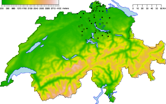
Figure 1: Map of Switzerland showing the stations of the 51 rainfall gauges used for the analysis, with an insert showing the altitude. The 36 stations marked by circles were used to fit the models, and those marked with squares were used to validate the models. Data for the pairs of stations with blue symbols appear in Figure 2.

1 Introduction

Natural hazards such as heat waves, high rainfall and snowfall, tides and windstorms, arise due to physical processes and are spatial in extent. Although it is difficult to attribute a particular event, such as Hurricane Katrina or the 2010 flooding in Pakistan, to the effects of climate change, both observational data and computer climate models suggest that the occurrence and sizes of such catastrophes will increase in the future. The potential consequences include increases in severe windstorms, flooding, wildfires, crop failure, population displacements and increased mortality. Apart from their direct impacts, such events will also have indirect effects such as increased costs for strengthening infrastructure and higher insurance premiums. There is thus a pressing need for a better understanding of spatial extremes and more detailed assessment of their consequences, and over the last few years the topic has become an active interface between climate, social and statistical scientists, in interaction with stakeholders such as insurance companies and public health officials. A particular issue when dealing with extremes is that although vast amounts of data may be available—though of varying quality and homogeneity—rare events are necessarily unusual and so the quantity of directly relevant data is limited. This difficulty is compounded in the spatial setting, because forecasting then entails extrapolation into a high-dimensional space, with all its attendant uncertainties. It is thus important that the statistical models used should both be flexible and have strong mathematical foundations, so that such extrapolation has an adequate basis. These requirements suggest the use of statistics of extremes, as sketched below.

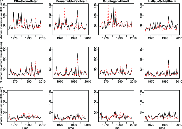
Figure 2: Annual, summer and winter maximum daily rainfall values for 1962–2008 at the four pairs of stations shown in blue in Figure 1. In each case the black line represents the station to the east and the red dashed line that to the west.

A variety of statistical tools have been used for the spatial modeling of extremes, including Bayesian hierarchical models, copulas and max-stable random fields. The purpose of this paper is to review and to compare these approaches in the practical context of modeling rainfall, with the twin goals of elucidating their properties and of contrasting them in a concrete context. To do this, we use summer maximum daily rainfall for the years 1962–2008 at 51 weather stations in the Plateau region of Switzerland, provided by the national meteorological service, MeteoSuisse. The stations lie north of the Alps and east of the Jura mountains, the largest and smallest distances between them being around 85 km and just over 3 km respectively. We randomly chose 35 stations to fit our models, and use the remaining 16 to validate them, as described below. The maximum and minimum distances between fitting and validation stations are very similar to those for all 51 stations. Their locations are shown in Figure 1; the region is relatively flat, the altitudes of the stations varying from 322 to 910 meters above mean sea level. Figure 2 shows the annual maxima and the maxima for the summer months, June–August, and for the winter months, December–February, for four pairs of stations marked in blue in Figure 1. As one would expect, there is a clear correlation among the maxima at these relatively short distances, and this must be reflected in the models if risk is to be accurately assessed.

In Section 2 we provide an overview of the parts of statistics of extremes that are needed later, and Section 3 provides a similar sketch of geostatistics. Subsequent sections describe latent variable, copula and max-stable approaches to the spatial modeling of extremes, which are then compared in Section 7. The paper ends with a brief discussion.

2 Statistics of Extremes

2.1 General

Statistics of extremes has grown into a vast field with many domains of application. Systematic mathematical accounts are given by Resnick (1987, 2007) and de Haan and Ferreira (2006), while more statistical treatments may be found in Beirlant et al. (2004), Coles (2001) and Embrechts, Klüppelberg and Mikosch (1997), the last focusing particularly on finance. Further reviews are provided by Kotz and Nadarajah (2000) and Finkenstädt and Rootzén (2004). A key issue in applications is that inferences may be required well beyond the observed tail of the data, and so an assumption of stability is required: mathematical regularities in the unobservable tail of the distribution are assumed to reach far enough back into the observable region that extrapolation may be based on a model fitted to the observed events. This requires an act of faith that the mathematics of regular variation, which underpins the extrapolation, is applicable in the practical circumstances in which the theory is applied. A statistical consequence of the lack of data is that tail inferences tend to be highly uncertain, and that the uncertainty can increase sharply as one moves further into the tail. In applications this can lead to alarmingly wide confidence intervals, but this seems to be intrinsic to the problem.

2.2 Univariate Models

Statistical modeling of extremes may be based on limiting families of distributions for maxima that satisfy the property of max-stability. At its simplest we take independent continuous scalar random variables $X_{1},\ldots,X_{m}\stackrel{{\scriptstyle\mathrm{iid}}}{{\sim}}F$, where the distribution $F$ has upper terminal $x_{F}=\sup\{x\dvtx F(x)<1\}$, and ask whether there exist sequences of constants $\{a_{m}\}>0$ and $\{b_{m}\}$ such that the rescaled variables

$$a_{m}^{-1}\{\max(X_{1},\ldots,X_{m})-b_{m}\}$$ (1)

have a nondegenerate limiting distribution $G$ as $m\to\infty$. It turns out that if such a $G$ exists, then it must be max-stable, that is, it must satisfy the equation

$$G^{m}(b^{\prime}_{m}+a^{\prime}_{m}y)=G(y),\quad y\in\mathbb{R},m\in\mathbb{N},$$ (2)

for sequences $\{a^{\prime}_{m}\}>0$ and $\{b^{\prime}_{m}\}$. The only nondegenerate distribution with this property is the generalized extreme-value (GEV) distribution

$$H(y)=\cases{\exp[-\{1+\xi{(y-\eta)/\tau}\}_{+}^{-1/\xi}],&$\xi\neq 0$,\cr\exp[-\exp\{-(y-\eta)/\tau\}],&$\xi=0$,}$$ (3)

where $u_{+}$ denotes $\max(u,0)$. The quantities $\eta$ and $\tau$ in (3) are respectively a real location parameter and a positive scale parameter; $\xi$ determines the weight of the upper tail of the density, with $\xi<0$ corresponding to the reverse Weibull case in which the support of the density has a finite upper bound, $\xi=0$ corresponding to the light-tailed Gumbel distribution, and $\xi>0$ corresponding to the heavy-tailed Fréchet distribution. The $r$th moment of $H$ exists only if $r\xi<1$.

Expression (3) is the broadest class of nondegenerate limit laws for a maximum $Y$ of a random sample of continuous scalar random variables, but in multivariate and spatial settings it is simpler to employ mathematically equivalent expressions that result from considering the transformed random variable $Z=\{1+\xi(Y-\eta)/\tau\}^{1/\xi}$, which has a unit Fréchet distribution $\exp(-1/z)$, for $z>0$. In this case the max-stability property may be written as $mZ\stackrel{{\scriptstyle D}}{{=}}\break\max(Z_{1},\ldots,Z_{m})$, where $Z,Z_{1},\ldots,Z_{m}$ represent mutually independent unit Fréchet random variables and $\stackrel{{\scriptstyle D}}{{=}}$ denotes equality in distribution. This transformation has the effect of separating the marginal GEV distributions of the variables from their joint dependence structure, and this is often convenient.

A typical goal in applications is the estimation of a high quantile of the distribution of $Y$, that is, a solution of the equation $H(y_{p})=p$; for $\xi\neq 0$ this is

$$y_{p}=\eta+\frac{\tau}{\xi}\{(-\log p)^{-\xi}-1\},\quad 0<p<1,$$

with the limit $\xi\to 0$ yielding $y_{p}=\eta-\tau\log(-\log p)$. If the available observations $Y_{j}$ are annual maxima and we set $p=1-1/T$, then $y_{p}$ is called the $T$-year return level, interpreted as the level exceeded once on average every $T$ years. Engineering requirements may be expressed in terms of $T$ or $y_{p}$. For example, the Dutch Delta Commission, responsible for protection against sea- and river-water flooding, set a risk level for sea flooding of North and South Holland that corresponds to a 10,000-year return level, and a risk level for river flooding that corresponds to a 1 250-year return level, though their physical interpretations in a nonstationary world are unclear. Estimates of $y_{p}$ are highly sensitive to $\xi$, and, if possible, it is helpful to pool information about this parameter.

Under mild conditions on the dependence structure of stationary time series, the GEV also emerges as the only possible nondegenerate limiting distribution for linearly renormalized maxima of blocks of observations, and this greatly widens its range of application; see Leadbetter, Lindgren and Rootzén (1983). In typical applications rare events occur in clusters whose mean size $\theta^{-1}$ is determined by the so-called extremal index, $\theta\in(0,1]$. Block maxima then have the GEV distribution $H(y)^{\theta}$, but the intra-cluster distribution may take essentially any form.

The discussion leading to (3) implies that forlarge $m$, $F(b_{m}+a_{m}y)^{m}\approx H(y)$, and, therefore, (2) implies that for large enough $x$,

$$F(x)\approx H^{1/m}\{(x-b_{m})/a_{m}\}\approx H(x)$$

for some choice of the parameters $\eta$, $\tau$ and $\xi$. Thus, although the generalized extreme-value distribu-tion (3) arises as the natural probability law for maxima of $m$ independent variables, it may also be regarded as giving an approximation for the upper tail of the distribution of an individual variable, provided a limiting distribution for maxima exists. For a high value $u<x_{F}$ and $x$ satisfying $u<x+u<x_{F}$, we therefore have

$$\operatorname{pr}(X>x+u\mid X>u)$$

$$\quad\approx\frac{1-H(x+u)}{1-H(u)}$$ (4)

$$\quad\approx(1+\xi x/{\sigma}_{u})_{+}^{-1/\xi},\quad x>0,$$

where ${\sigma}_{u}=\tau+\xi(u-\eta)$. The last expression in (2.2) is the survivor function of the generalized Pareto distribution (GPD), which is commonly used for modeling exceedances over high thresholds (Davison and Smith (1990)). The standard approach to such modeling presupposes that the times of exceedances over the high threshold $u$ are the realization of a stationary Poisson process of rate $\lambda$, say, and that their sizes are independent with survivor function (2.2). This model may also be formulated in terms of a limiting Poisson process of extremes (Smith (1989)).

2.3 Multivariate Models

We now consider componentwise maxima of an independent sequence of bivariate random variables $(X_{1i},X_{2i})$, for $i=1,\ldots$ . If nondegenerate limiting marginal distributions exist, these must be of the form (3), and, hence, the rescaled limiting versions of the componentwise maxima $\max(X_{11},\ldots,X_{1n})$ and $\max(X_{21},\ldots,X_{2n})$ may be transformed to have marginal unit Fréchet distributions. It turns out that if it exists and is nondegenerate, then the limiting joint distribution of the transformed componentwise maxima can be written as

$$\operatorname{pr}(Z_{1}\leq z_{1},Z_{2}\leq z_{2})$$

(5)

$$\quad=\exp\{-V(z_{1},z_{2})\},\quad z_{1},z_{2}>0,$$

where the exponent measure $V(z_{1},z_{2})$ (Resnick(1987), page 268) satisfies

$$V(z_{1},\infty) = 1/z_{1},\quad V(\infty,z_{2})=1/z_{2},$$

$$V(tz_{1},tz_{2}) = t^{-1}V(z_{1},z_{2}),\quad t>0.$$

Here the first two properties ensure that the marginal distributions are unit Fréchet, and the third shows that the function $V$ is homogeneous of order $-1$, thereby extending the max-stability property to the bivariate case. This argument extends to multivariate extremes, for which the corresponding function $V(z_{1},\ldots,z_{D})$ satisfies the analogues of (2.3). Twobounding cases are where $Z_{1},\ldots,Z_{D}$ are independent or are entirely dependent, corresponding respectively to

$$V(z_{1},\ldots,z_{D}) = 1/z_{1}+\cdots+1/z_{D},$$

$$V(z_{1},\ldots,z_{D}) = 1/\min(z_{1},\ldots,z_{D}).$$

A consequence of the homogeneity of $V$ is that multivariate extreme-value distributions have various so-called spectral representations, of which the best-known, due to Pickands (1981), rewrites the exponent measure as

$$V(z_{1},\ldots,z_{D})$$

$$\quad=\int_{{\mathcal{S}}_{D}}\max(w_{1}/z_{1},\ldots,w_{D}/z_{D})$$ (7)

$$\hphantom{\quad=\int_{{\mathcal{S}}_{D}}}dM(w_{1},\ldots,w_{D}),$$

where $M$ is a measure on the $D$-dimensional simplex ${\mathcal{S}}_{D}$. On setting all but one of the $z_{d}$ equal to $+\infty$, we see that in order for the distribution to have unit Fréchet margins, $M$ must satisfy the constraint $\int w_{d}\,dM(w_{1},\ldots,w_{D})=1$ for each $d$. Unlike for univariate extremes, there is no simple parametric form for the multivariate limiting distribution; $V$ can take any form subject to (2.3). From a statistical viewpoint this is a mixed blessing. Although numerous parametric forms for $V$ or equivalent functions have been proposed (Kotz and Nadarajah (2000), Section 3.5), those in current use tend to be somewhat inflexible, and, owing to the curse of dimensionality, nonparametric estimation has essentially been confined to the bivariate case (Fougères (2004); Boldi and Davison (2007); Einmahl and Segers (2009)). More positively, we may use the flexibility to construct functions $V$ adapted to specific applications.

A difficulty for statistical inference arises because equations such as (2.3) specify cumulative distribution functions. The likelihood function for $D$-dimensional data involves differentiation of $\exp\{-V(z_{1},\ldots,z_{D})\}$ with respect to $z_{1},\ldots,z_{D}$, resulting in a combinatorial explosion; the number of terms is the number of partitions of the integer $D$. Even for only ten dimensions, $D=10$, a single likelihood evaluation would involve a sum of over 100,000 different terms, which seems infeasible in general, though there may be simplifications in special cases.

2.4 Extremal Coefficient

It is useful to have summary measures of extremal dependence. One possibility is based on the probability that all the transformed variables are less than $z$,

$$\operatorname{pr}(Z_{1}\leq z,\ldots,Z_{D}\leq z)$$

$$\quad=\exp\{-V(1,\ldots,1)/z\}$$ (8)

$$\quad=\exp(-\theta_{\mathcal{D}}/z),\quad z>0,$$

owing to the homogeneity of $V$. The quantity $\theta_{\mathcal{D}}$, known as the extremal coefficient of the observations $Z_{d}$, $d\in{\mathcal{D}}=\{1,\ldots,D\}$, varies from $\theta_{\mathcal{D}}=1$ when the observations are fully dependent to $\theta_{\mathcal{D}}=D$ when they are independent, and thus provides a summary of the degree of dependence, though it does not determine the joint distribution. In the bivariate case it is easy to check that

$$\lim_{z\to\infty}\operatorname{pr}(Z_{2}>z\mid Z_{1}>z)=2-\theta_{\mathcal{D}},$$

thereby providing an interpretation of $\theta_{\mathcal{D}}$ in terms of the limiting probability of an extreme event in one variable, given a correspondingly rare event in the other. Thus, if $\theta_{\mathcal{D}}=2$, this probability is zero, while smaller values of $\theta_{\mathcal{D}}$ will yield larger conditional probabilities.

Schlather and Tawn (2003) discuss the consistency properties that must be satisfied by the extremal coefficients of subsets of $Z_{1},\ldots,Z_{D}$, and suggest how these coefficients may be estimated. Below we compare purely empirical estimators for pairs of sites with the fitted versions found from models, so we need to estimate $\theta_{\mathcal{D}}$ for $D=2$. In our experience madogram estimators perform well, and we use these below. The $F$-madogram is defined as (Cooley,Naveau and Poncet (2006))

$$\nu_{F}=\tfrac{1}{2}{\mathrm{E}}\{|F(Z_{1})-F(Z_{2})|\},$$ (9)

where $F(z)=\exp(-1/z)$. Unlike the more common variogram (Schabenberger and Gotway (2005), Chapter 4), (9) remains finite when the margins of the process are heavy tailed, because ${\mathrm{E}}\{F^{k}(Z_{1})\}=1/\allowbreak(1+k)$, for $k>0$, and it has a bijective relationship with the extremal coefficient $\theta={(1+2\nu_{F})/(1-2\nu_{F})}$. Cooley, Naveau and Poncet (2006) discuss estimation of the extremal coefficient based on the madogram, which is extended by Naveau et al. (2009) to the setting in which maxima of a stationary process are observed at many points in space and it is required to estimate the extremal coefficient as a function of the distance between them.

3 Geostatistics

3.1 Generalities

Geostatistics is a large and rapidly developing domain of statistics, with important applications in areas such as public health, agriculture and resource exploration, and in environmental and ecologicalstudies. Standard texts are Cressie (1993), Stein(1999), Wackernagel (2003), Banerjee, Carlin and Gelfand (2004), Schabenberger and Gotway (2005) and Diggle and Ribeiro (2007). There are three common data types: spatial point processes, used to model data whose observation sites may be treated as random; areal data, available at a set of sites for which interpolation may be uninterpretable, such as climate model output; and point-referenced or geostatistical data, which may be modeled as values from a spatial process defined on the continuum but observed only at fixed sites, between which interpolation makes sense.

=340pt Family Correlation function Range of validity Whittle–Matérn $\rho(h)=\{2^{\kappa-1}\Gamma(\kappa)\}^{-1}(\|h\|/\lambda)^{\kappa}K_{\kappa}(\|h\|/\lambda)$ $\kappa>0$ Cauchy $\rho(h)=\{1+(\|h\|/\lambda)^{2}\}^{-\kappa}$ $\kappa>0$ Stable $\rho(h)=\exp\{-(\|h\|/\lambda)^{\kappa}\}$ $0<\kappa\leq 2$ Exponential $\rho(h)=\exp(-\|h\|/\lambda)$ –

Table 1: Parametric families of isotropic correlation functions. Here $K_{\kappa}$ denotes the modified Bessel function of order $\kappa$ and $\Gamma(u)$ denotes the gamma function. In each case $\lambda>0$

Here we are concerned with point-referenced data, for which a suitable mathematical model is a random process $\{Y(x)\}$ defined at all points $x$ of a spatial domain ${\mathcal{X}}$, typically taken to be a contiguous subset of $\mathbb{R}^{2}$. Examples are levels of air pollution or annual maximum temperatures observed at a finite subset ${\mathcal{D}}=\{x_{1},\ldots,x_{D}\}$ of sites of ${\mathcal{X}}$. The statistical problem is to make inference for the process elsewhere in ${\mathcal{X}}$. Having observed daily rainfall depths $Y(x_{1}),\ldots,Y(x_{D})$ at a set of weather stations, for example, we may wish to predict $Y(x)$ at an unobserved site $x$, estimate the highest depth $\sup_{x\in{\mathcal{X}}}Y(x)$ in the region, or provide a distribution for a quantity such as $\int_{x\in{\mathcal{X}}}Y(x)\,dx$. Below we sketch elements of geostatistics needed subsequently, leaving the interested reader to consult the references above for further details.

3.2 Gaussian Processes

The simplest and best-explored approach to modeling point-referenced data is to suppose that $\{Y(x)\}$ follows a Gaussian process defined on ${\mathcal{X}}$. Such a process is called intrinsically stationary if, in addition to its finite-dimensional distributions being Gaussian, its increments are stationary, that is, the process $\{Y(x+h)-Y(x)\dvtx x\in{\mathcal{X}}\}$ is stationary for all lag vectors $h$. Then we take ${\mathrm{E}}\{Y(x+h)-Y(x)\}=0$, and there exists a function

$$\gamma(h)=\tfrac{1}{2}\operatorname{var}\{Y(x+h)-Y(x)\},\quad x,x+h\in{\mathcal{X}},$$

called the semivariogram; this need not be bounded. A stronger assumption is that of second-order stationarity, meaning that $\operatorname{var}\{Y(x)\}$ is a finite constant for $x\in{\mathcal{X}}$ and that the covariance function $\operatorname{cov}\{Y(x_{1}),Y(x_{2})\}$ exists and may be expressed as $C(x_{1}-x_{2})$, where $C(\cdot)$ is a positive definite function. In this case we may write $\gamma(h)=C(0)-C(h)$, and we see that $\gamma(h)$ is bounded above by $C(0)=\operatorname{var}\{Y(x)\}$ and that $\rho(h)=C(h)/C(0)$ is a correlation function. For Gaussian processes second-order stationarity is equivalent to stationarity, under which the joint distribution of any finite subset of points of $Y(x)$ depends only on the vectors between their sites.

Gneiting, Sasvári and Schlather (2001) discuss the relationships between semivariograms and covari-ance functions: in particular, a real function on $\mathbb{R}^{2}$ satisfying $\gamma(0)=0$ is the semivariogram of an intrinsically stationary process if and only if it is conditionally negative definite, that is,

$$\sum_{i,j=1}^{n}a_{i}a_{j}\gamma(x_{i}-x_{j})\leq 0$$ (10)

for all finite sets of sites $x_{1},\ldots,x_{n}$ in ${\mathcal{X}}$ and for all sets of real numbers $a_{1},\ldots,a_{n}$ summing to zero, or, equivalently, if $\exp\{-t\gamma(h)\}$ is a covariance function for all $t>0$. Clearly, a semivariogram or covariance function valid in $\mathbb{R}^{p}$ is also valid in lower-dimensional spaces, though the converse is false.

A covariance function or, equivalently, a semivariogram is called isotropic if it depends only on the length $\|x_{1}-x_{2}\|$ of $x_{1}-x_{2}$ and not on its orientation; this typically unrealistic but very convenient modeling assumption imposes additional restrictionson $\gamma(h)$.

Schabenberger and Gotway [(2005), Section 4.3] and Banerjee, Carlin and Gelfand [(2004), Sec-tion 2.1] describe a variety of valid correlation functions. Isotropic forms for those used in this paper are summarized in Table 1, where $\lambda$ represents a positive scale parameter with the dimensions of distance, and $\kappa$ is a shape parameter that controls the properties of the random process and, in particular, can determine the roughness of its realizations. The Whittle–Matérn family is flexible and widely used in practice, though it is often difficult to estimate its shape parameter. A simple way to add anisotropy to such functions is to replace $\|h\|$ by $(h^{\mathrm{T}}Ah)^{1/2}$, where $A$ is a positive definite matrix with unit determinant; this is known as geometric anisotropy.

If $\{{\varepsilon}(x)\}$ and $\{{\varepsilon}^{\prime}(x)\}$ are two independent stationary Gaussian processes with unit variance and correlation functions $\rho(h)$ and $\rho^{\prime}(h)$, then their sum is also a Gaussian process, with correlation function $\rho(x)+\rho^{\prime}(x)$. A white noise process $\{{\varepsilon}^{\prime}(x)\}$ has correlation function $\rho(h)=\delta(h)$, where $\delta(h)$ denotes the Kronecker delta function, and thus the process $\{{\sigma}(1-\alpha)^{1/2}{\varepsilon}(h)+{\sigma}\alpha^{1/2}{\varepsilon}^{\prime}(h)\}$ has variance ${\sigma}^{2}$ and correlation function $(1-\alpha)\rho(h)$ for $h\neq 0$; there is a so-called nugget effect at the origin, corresponding to the extremely local variation added by the white noise. In this case a proportion $\alpha$ of the variance arises from this nugget effect.

4 Latent Variable Models

4.1 General

Dependence in many statistical settings is introduced by integration over latent variables or processes. Here this idea can be used to introduce spatial variation in the parameters. For example, we may suppose that the response variables $\{Y(x)\}$ are independent conditionally on an unobserved latent process $\{S(x)\dvtx x\in\mathcal{X}\}$, let the parameters of the response distributions depend on $\{S(x)\}$, suppose that $\{S(x)\}$ follows a Gaussian process, and then induce dependence in $\{Y(x)\}$ by integration over the latent process. This approach is common in geostatistics with nonnormal response variables (Diggle, Tawn and Moyeed (1998); Diggle and Ribeiro (2007)), and because of the complexity of the integrations involved is most naturally performed in a Bayesian setting, using Markov chain Monte Carlo algorithms (Gilks, Richardson and Spiegelhalter(1996); Robert and Casella (2004)) to perform inferences. An excellent account of this approach to spatial modeling is provided by Banerjee, Carlin and Gelfand (2004).

The first application of latent variables to statistical extremes was the study of hurricane wind speeds by Coles and Casson (1998) and Casson and Coles (1999). They treated position on the Eastern seaboard of the US as a scalar spatial variable and used a hierarchical Bayes model with a stable correlation function to fit the point process likelihood to their data. In their application the main gains relative to treating the data at different sites as independent were the possibility of interpolation of the distribution of extreme wind speeds between sites at which they had been observed, and an increase in the precision of estimation due to borrowing of strength. A related approach, but without spatial structure, was used by Fawcett and Walshaw (2006) to model wind speeds in central and northern England.

Cooley, Nychka and Naveau (2007) used the generalized Pareto model (2.2) with a common threshold $u$ at all sites to map return levels for extreme rainfall in Colorado. The rate parameter $\lambda$ and the scale parameter $\sigma_{u}$ depended on location $x$ in a climate space comprised of elevation above sea-level and mean precipitation, instead of longitude and latitude. A stationary isotropic exponential covariance function was used to induce spatial dependence in the latent processes $\{S(x)\}$ for these parameters. The shape parameter $\xi$ had two values, depending on the site location. Turkman, Turkman and Pereira (2010) construct a similar but more complex model for space-time properties of wildfires in Portugal, using a random walk to describe the temporal properties, and smoothing for the spatial dependence; their paper also makes suggestions on spatial max-stable modeling with exceedances. Gaetan and Grigoletto (2007) analyze annual rainfall maxima at sites in northeastern Italy, using nonstationary spatial dependence and random temporal trend in the parameters of the generalized extreme-value distribution. Sang and Gelfand (2009) modeled gridded annual rainfall maxima in the Cape Floristic Region of South Africa using the generalized extreme-value distribution with a spatio-temporal hierarchical structure, and in Sang and Gelfand (2010) used a Gaussian spatial copula model, transformed to the generalized extreme-value scale, to induce dependence between extremes of point-referenced rainfall data. Other applications of such models to areal data are Cooley and Sain (2010), who assessed possible changes in rainfall extremes by comparing current and future rainfall computed from a regional climate model, using an intrinsic autoregression to model how the three parameters of the point process formulation for extremes vary on a large grid. Owing to difficulties in estimating the shape parameter, these authors used a penalty due to Martins and Stedinger (2000) to ensure that $|\xi|<1/2$.

In the next section we describe a rather simpler latent model for the annual maximum rainfall data used in this paper.

4.2 A Simple Model

Suppose that the GEV parameters $\{\eta(x),\tau(x),\allowbreak\xi(x)\}$ vary smoothly for $x\in\mathcal{X}$ according to a stochastic process $\{S(x)\}$. For our application, and by analogy with Casson and Coles (1999), we assume that the Gaussian processes for each GEV parameter are mutually independent, though this assumption can be relaxed (Sang and Gelfand (2009); Cooley and Sain (2010)). For instance, we take

$$\eta(x)=f_{\eta}(x;\bolds{\beta}_{\eta})+S_{\eta}(x;\alpha_{\eta},\lambda_{\eta}),$$ (11)

where $f_{\eta}$ is a deterministic function depending on regression parameters $\bolds{\beta}_{\eta}$, and $S_{\eta}$ is a zero mean, stationary Gaussian process with covariance function $\alpha_{\eta}\exp(-\|h\|/\lambda_{\eta})$ and unknown sill and range parameters $\alpha_{\eta}$ and $\lambda_{\eta}$. We use similar formulations for $\tau(x)$ and $\xi(x)$. Then conditional on the values of the three Gaussian processes at the sites $(x_{1},\ldots,\allowbreak x_{D})$, the maxima are assumed to be independent with

$$Y_{i}(x_{d})\mid\{\eta(x_{d}),\tau(x_{d}),\xi(x_{d})\}$$

$$\quad\sim\operatorname{GEV}\{\eta(x_{d}),\tau(x_{d}),\xi(x_{d})\},$$

$$\hskip 53.0pt\quad\quad i=1,\ldots,n,d=1,\ldots,D.$$

A joint prior density $\pi$ must be defined for the parameters $\alpha_{\eta}$, $\alpha_{\tau}$, $\alpha_{\xi}$, $\lambda_{\eta}$, $\lambda_{\tau}$, $\lambda_{\xi}$, $\bolds{\beta}_{\eta}$, $\bolds{\beta}_{\tau}$ and $\bolds{\beta}_{\xi}$. In order to reduce the computational burden, we use conjugate priors whenever possible, taking independent inverse Gamma and multivariate normal distributions for $\alpha_{\tau}$ and $\bolds{\beta}_{\tau}$, respectively. No conjugate prior exists for $\lambda_{\tau}$, for which we take a relatively uninformative Gamma distribution. The prior distributions for the two remaining GEV parameters are defined similarly. The full conditional distributions needed for Markov chain Monte Carlo computation of the posterior distributions are as follows:

$$\pi(\bolds{\eta}\mid\cdots) \propto \pi(\bolds{\eta}\mid\alpha_{\eta},\lambda_{\eta},\bolds{\beta}_{\eta})\pi(\mathbf{y}\mid\bolds{\eta},\bolds{\tau},\bolds{\xi}),$$

$$\pi(\alpha_{\eta}\mid\cdots) \propto \pi(\alpha_{\eta}\mid\kappa_{\alpha_{\eta}}^{*},\theta_{\alpha_{\eta}}^{*})\pi(\bolds{\eta}\mid\alpha_{\eta},\lambda_{\eta},\bolds{\beta}_{\eta}),$$

$$\pi(\lambda_{\eta}\mid\cdots) \propto \pi(\lambda_{\eta}\mid\kappa_{\lambda_{\eta}}^{*},\theta_{\lambda_{\eta}}^{*})\pi(\bolds{\eta}\mid\alpha_{\eta},\lambda_{\eta},\bolds{\beta}_{\eta}),$$

$$\pi(\bolds{\beta}_{\eta}\mid\cdots) \propto \pi(\bolds{\beta}_{\eta}\mid\mu_{\eta}^{*},\Sigma_{\eta}^{*})\pi(\bolds{\eta}\mid\alpha_{\eta},\lambda_{\eta},\bolds{\beta}_{\eta}),$$

where $\kappa_{\cdot}^{*}$, $\theta_{\cdot}^{*}$, $\mu_{\cdot}^{*}$ and $\Sigma_{\cdot}^{*}$ are the hyperparameters of the prior distributions. The full conditional distributions related to $\bolds{\tau}$ and $\bolds{\xi}$ have similar expressions. The corresponding Markov chain Monte Carlo algorithm is outlined in the Appendix.

5 Copula Models

5.1 Generalities

In view of the flexibility of modeling afforded by Gaussian-based geostatistical models, and, in particular, the range of potential covariance functions, it is natural to investigate how they may be extended to model spatial extremes. An obvious approach is to use the probability integral transformation to place the annual maxima on the Gaussian scale, on which their joint distribution can be modeled using standard geostatistical tools. However, the requirement that the model for the original data should be max-stable imposes tight restrictions on the possible covariance structures, even on the Gaussian scale. Although these restrictions are theoretical in nature, we shall see below that they strongly affect the fit of the models. There is a close relationship between this approach and the use of copulas, and we first give a brief outline of the latter.

5.2 Copulas

Sklar’s Theorem (Nelsen (2006), pages 17–24) establishes that the $D$-dimensional joint distribution $F$ of any random vector $Y_{1},\ldots,Y_{D}$ may be written as

$$\quad F(y_{1},\ldots,y_{D})=C\{F_{1}(y_{1}),\ldots,F_{D}(y_{D})\},$$ (13)

where $F_{1},\ldots,F_{D}$ are the univariate marginal distributions of $X_{1},\ldots,X_{D}$ and $C$ is a copula, that is, a $D$-dimensional distribution on $[0,1]^{D}$. The function $C$ is uniquely determined for distributions $F$ with absolutely continuous margins. If the marginal distributions $F_{d}$ are continuous and strictly increasing, then $C$ corresponds to the distribution of $F_{1}(Y_{1}),\allowbreak\ldots,F_{D}(Y_{D})$, that is,

$$C(u_{1},\ldots,u_{D})=F\{F_{1}^{-1}(u_{1}),\ldots,F_{D}^{-1}(u_{D})\}.$$

Nelsen (2006) and Joe (1997) are clear introductions to multivariate models and copulas.

One might argue, with Mikosch (2006), that the transformation to uniform margins is mathematically trivial, obscures important features of the data that are visible on their original scale and makes stochastic modeling awkward, and hence is rarely interesting for applications. An alternative view is that the implicit separation of the marginal distributions of the variables from their dependence structure provides a unifying framework to modeling multivariate data. The discussion following Mikosch’s paper may be consulted for a lively debate of the merits and demerits of copulas; here we merely wish to show how they may be used to model spatial extremes.

As a simple and important example, suppose that $Y_{1},\ldots,Y_{D}$ have a joint Gaussian distribution with means zero and covariance matrix $\Omega$ whose diagonal elements all equal unity. The Gaussian copula function is

$$\quad C(u_{1},\ldots,u_{D})=\Phi\{\Phi^{-1}(u_{1}),\ldots,\Phi^{-1}(u_{D});\Omega\},$$ (14)

where $\Phi(\cdot;\Omega)$ is the joint distribution function of $Y_{1},\ldots,Y_{D}$ and $\Phi$ denotes the cumulative distribution function of a standard normal random variable. Here we have used the componentwise transformation $U_{i}=\Phi(Y_{i})$. The corresponding density is readily obtained. Similarly, the copula of the multivariate Student $t$ distribution with $\nu$ degrees of freedom and dispersion matrix $\Omega$ may be written

$$C(u_{1},\ldots,u_{D})$$

(15)

$$\quad=T_{\nu}\{T^{-1}_{\nu}(u_{1}),\ldots,T^{-1}_{\nu}(u_{D});\Omega\},$$

where $T_{\nu}(\cdot;\Omega)$ and $T_{\nu}$ are the corresponding joint and marginal distribution functions.

5.3 Extremal Copulas

If the random variables $Y_{1},\ldots,Y_{D}$ possess a joint multivariate extreme value distribution, then their marginal distributions are of the form (3). As these margins are continuous, equation (13) implies that the joint distribution must correspond to a unique copula, and the max-stability property implies that this copula must satisfy

$$C(u_{1}^{m},\ldots,u_{D}^{m})$$

$$\quad=C^{m}(u_{1},\ldots,u_{D}),\quad 0<u_{1},\ldots,u_{D}<1,\ m\in\mathbb{N}.$$

Such a copula, called an extremal copula or stable dependent function (Galambos (1987); Joe (1997)), is closely related to the exponent measure of Section 2.3, through the relation $C(u_{1},\ldots,u_{D})=\break\exp\{-V(-1/\log u_{1},\ldots,-1/\log u_{D})\}$. The spectral representation (2.3) means that we may write

$$C(u_{1},\ldots,u_{D})$$

$$\quad=\exp\Biggl{\{}A\biggl{(}\frac{\log u_{1}}{\sum\log u_{d}},\ldots,\frac{\log u_{D}}{\sum\log u_{d}}\biggr{)}$$ (16)

$${}\hskip 92.0pt\quad\quad\times\sum_{d=1}^{D}\log u_{d}\Biggr{\}},$$

where the function $A$, called the the Pickands dependence function, depends on the measure $M$ on the simplex ${\mathcal{S}}_{D}$; $A$ is often written as a function of just $D-1$ of its arguments, which sum to unity. Since the transformation from Fréchet to uniform margins is continuous, convergence of rescaled maxima to a nondegenerate joint limiting distribution on the uniform scale follows from the convergence on the Fréchet scale. A useful example is the extremal $t$ copula (Demarta and McNeil (2005)), which results from rescaling the maxima of independent multivariate Student $t$ variables with dispersion matrix $\Omega$ and $\nu$ degrees of freedom. For $D=2$ this yields

$$\quad A(w) = wT_{\nu+1}\biggl{[}{\{w/(1-w)\}^{1/\nu}-\rho\over\{(1-\rho^{2})/(\nu+1)\}^{1/2}}\biggr{]}$$

$${}+(1-w)T_{\nu+1}\biggl{[}{\{(1-w)/w\}^{1/\nu}-\rho\over\{(1-\rho^{2})/(\nu+1)\}^{1/2}}\biggr{]},$$

$$\hskip 74.0pt\quad 0<w<1,-1<\rho<1,$$

where $\rho$ is the correlation obtained from $\Omega$. The limit of (5.3) when the correlation may be expressed as $\rho=\exp\{-a^{2}/(2\nu)\}\sim 1-a^{2}/(2\nu)$ for some $a>0$ and $\nu\to\infty$ is the Hüsler and Reiss (1989) copula given by

$$\qquad A(w) = (1-w)\Phi\biggl{\{}{a\over 2}+a^{-1}\log\biggl{(}{1-w\over w}\biggr{)}\biggr{\}}$$

$${}+w\Phi\biggl{\{}{a\over 2}+a^{-1}\log\biggl{(}{w\over 1-w}\biggr{)}\biggr{\}},$$

$$\hskip 121.0pt\quad 0<w<1;$$

see also Nikoloulopoulos, Joe and Li (2009). This implies that the extremal $t$ copula is more flexible than the Hüsler–Reiss copula, in two distinct ways: first, the presence of the degrees of freedom introduces a further parameter; second, two different correlation functions that yield the same form for $a$ when $\nu\to\infty$, such as the Gaussian function $\rho(h)=\exp\{-(h/\lambda)^{2}/(2\nu)\}$ and the Cauchy function $\rho(h)=\{1+(h/\lambda)^{2}/(2\nu)\}^{-\kappa}$, will both yield the same form for (5.3) but not for (5.3). In the limit as $\nu\to\infty$ the parameter $\kappa$ must be absorbed by reparametrization, as we shall see in Section 7.3. Owing to the relationship between correlation functions and variograms mentioned after (10), we see that $a^{2}$ will correspond to a semivariogram.

For any fixed correlation $|\rho|\!<\!1$, it follows from (5.3) that the limit as $\nu\to\infty$ is $A(w)=1$, which corresponds to $C(u_{1},u_{2})=u_{1}u_{2}$, so componentwise maxima of correlated normal variables are independent in the limit, except in the trivial case $|\rho|=1$. A similar limit with a different rescaling was used by Hüsler and Reiss (1989) when taking maxima of $m$ independent bivariate Gaussian variables with correlation $\rho$; in this case letting $\rho\to 1$ such that $\lim_{m\to\infty}4(1-\rho)\log m=a^{2}$ also yields (5.3).

The limit of (5.3) when $\nu\to 0$ is the Marshall–Olkin copula

$$C(u_{1},u_{2})$$

$$\quad=\exp\{\alpha\log(u_{1}u_{2})+(1-\alpha)\log\min(u_{1},u_{2})\},$$

$$\hskip 160.0pt\quad 0\leq\alpha\leq 1,$$

where $\alpha=T_{1}\{-\rho/(1-\rho^{2})^{1/2}\}$. The boundary cases in (5.3) are $\alpha=0$, which corresponds to perfectly dependent extremes and arises for $\rho=1$, and $\alpha=1$, which corresponds to independent extremes andarises for $\rho=-1$.

5.4 Tail Dependence

Pairwise tail dependence in copulas may be measured using the limits of the conditional probabilities $\operatorname{pr}(U_{2}>u\mid U_{1}>u)$ and $\operatorname{pr}(U_{2}\leq u\mid U_{1}\leq u)$, which may be written as

$$\chi_{\rm up} = \lim_{u\to 1-}{1-2u-C(u,u)\over 1-u},$$

$$\chi_{\rm low} = \lim_{u\to 0+}{C(u,u)\over u},$$

provided that these limits exist. If one of these expressions is positive, then there is dependence in the corresponding tail, and otherwise there is independence. If an extremal copula $C^{*}$ corresponding to $C$ exists and is nondegenerate, that is, if

$$C(u_{1}^{1/m},u_{2}^{1/m})^{m}\to C^{*}(u_{1},u_{2}),$$

$$\hskip 61.0pt\qquad 0<u_{1},u_{2}<1,m\to\infty,$$

then the values of $\chi_{\rm up}$ for $C$ and $C^{*}$ are equal (Joe (1997), page 178).

In the max-stable case there is a close relation between $\chi_{\rm up}$ and the extremal coefficient, $\theta$, viz., $\chi_{\rm up}=2-\theta=2-2A(1/2,1/2)$, where $A$ is the dependence function in (5.3). In particular, the Gaussian copula has $\chi_{\rm up}=\chi_{\rm low}=0$, the Student $t$ copula has

$$\chi_{\rm up}=\chi_{\rm low}=2T_{\nu+1}\biggl{[}-\biggl{\{}{(\nu+1)(1-\rho)\over 1+\rho}\biggr{\}}^{1/2}\biggr{]},$$

whose symmetry stems from the elliptical form of the joint densities, and the Hüsler–Reiss copula has $\chi_{\rm up}=2-2\Phi(a/2)$ and $\chi_{\rm low}=0$.

5.5 Inference

Given data $y_{1},\ldots,y_{D}$ assumed to be a realization from a multivariate distribution whose margins take the parametric forms $H_{1}(y;\zeta),\ldots,H_{D}(y;\zeta)$ and which has a parametric copula $C$ that depends upon parameters $\gamma$, the parameter vector $\vartheta=(\zeta,\gamma)$ may be estimated by forming a likelihood from the joint density corresponding to the joint distribution$C\{H_{1}(y_{1};\zeta),\ldots,H_{D}(y_{D};\zeta);\gamma\}$. In the spatial context the $H_{d}$ will typically depend on the site $x_{d}$ at which $y_{d}$ is observed, as in (4.2), and $\gamma$ will represent the parameters of a function that controls how the dependence of $y_{c}$ and $y_{d}$ is related to the distance between them. For example, when fitting the Student $t$ copula, the $(c,d)$ element of the dispersion matrix $\Omega$ could be of the form ${\sigma}^{2}\rho(x_{c}-x_{d})$, where $\rho$ is one of the correlation functions of Section 3.2.

If the joint density of $Y_{1},\ldots,Y_{D}$ is available, then likelihood inference may be performed in the usual way, with the observed information matrix used to provide standard errors for estimates based on large samples, and information criteria used to compare competing models. Alternatively, Bayesian inference can be performed; for example, Sang and Gelfand (2010) use Markov chain Monte Carlo to fit such a model, with the Gaussian copula, exponential correlation function and GEV marginal distributions having the same scale and shape parameters but a regression structure and spatial random effects in the location parameter. Unfortunately the joint density of $Y_{1},\ldots,Y_{D}$ is not available when using the Hüsler–Reiss and extremal $t$ copulas, for which only the bivariate distributions corresponding to (5.3)and (5.3) are known. In Section 6.2 we discuss the use of composite likelihood for inference in such cases.

6 Max-Stable Models

6.1 Models

It is natural to ask whether there are useful spatial extensions of the extremal models described in Section 2. The central arguments of Section 2.2 were extended to the process setting by Laurens de Haan around three decades ago, and a detailed account is given by de Haan and Ferreira (2006), Chapter 9. A key notion is that of a so-called spectral representation of extremal processes, and for our purposes the most useful such representation is due to Schlather (2002). Let $\{S^{-1}_{j}\}_{j=1}^{\infty}$ be the points of a homogeneous Poisson process of unit rate on $\mathbb{R}_{+}$, so that $\{S_{j}\}_{j=1}^{\infty}$ are the points of a Poisson process on $\mathbb{R}_{+}$ with intensity $ds/s^{2}$, and let $\{W_{j}(x)\}_{j=1}^{\infty}$ be independent replicates of a stationary process $W(x)$ on $\mathbb{R}^{p}$ satisfying ${\mathrm{E}}[\max\{0,W_{j}(o)\}]=1$, where $o$ denotes the origin. Then

$$Z(x)=\max_{j}S_{j}\max\{0,W_{j}(x)\}$$ (20)

is a stationary max-stable process on $\mathbb{R}^{p}$ with unit Fréchet marginal distributions. To see this, note following Smith (1990) that we can consider the$\{S_{j},W_{j}(x)\}_{j=1}^{\infty}$ to be the points in a Poisson process of intensity $ds/s^{2}\times\nu(dw)$ on $\mathbb{R}_{+}\times{\mathcal{W}}$, where $\nu$ is the measure of the $W_{j}(x)$ and ${\mathcal{W}}$ is a suitable space. Thus, the probability that $Z(x)\leq z$ equals the void probability of the set $\{(s,w)\in\mathbb{R}_{+}\times{\mathcal{W}}\dvtx\break s\max(0,w)>z\}$, which has measure

$$\int\int_{z/\max\{0,w\}}^{\infty}{ds\over s^{2}}\nu(dw) = \int z^{-1}\max\{0,w\}\nu(dw)$$

$$= z^{-1}$$

because ${\mathrm{E}}[\max\{0,W_{j}(o)\}]=1$; hence, $Z(x)$ has a unit Fréchet distribution. The max-stability follows from the infinite divisibility of the Poisson process, which implies that the distributions of $\{\max_{j=1,\ldots,m}Z_{j}(x_{1}),\allowbreak\ldots,\max_{j=1,\ldots,m}Z_{j}(x_{D})\}$ and $m\{Z(x_{1}),\ldots,Z(x_{D})\}$ are equal for any finite subset of points $\{x_{1},\ldots,\break x_{D}\}\subset{\mathcal{X}}$.

Different choices for the process $W(x)$ lead to some useful max-stable models. Stationarity implies that if we wish to describe the joint distributions of the max-stable process $\{Z(x)\}$ at pairs of points of ${\mathcal{X}}$, then there is no loss of generality in considering the sites $o$ and $h$, and for the remainder of this subsection we describe the joint distributions of $Z(o)$ and $Z(h)$ under some simple models.

A first possibility is to take $W_{j}(x)=g(x-X_{j})$, where $g$ is a probability density function and $\{X_{j}\}$ is a homogeneous Poisson process, both on $\mathbb{R}^{p}$. In this case the value of the max-stable process at $x$ may be interpreted as the maximum over an infinite number of storms, centered at the random points $X_{j}$ and of ferocities $S_{j}$, whose effects at $x$ are given by $S_{j}g(x-X_{j})$. The case where $g$ is the normal density was considered by Smith (1990) in a pioneering unpublished report and is often called the Smith model. If $g$ is taken to be the multivariate normal distribution with covariance matrix $\Omega$, then the exponent measure for $Z(o)$ and $Z(h)$ is

$$z_{1}^{-1}\Phi\biggl{\{}{a(h)\over 2}+a^{-1}(h)\log\biggl{(}{z_{2}\over z_{1}}\biggr{)}\biggr{\}}$$

(21)

$${}\quad+z_{2}^{-1}\Phi\biggl{\{}{a(h)\over 2}+a^{-1}(h)\log\biggl{(}{z_{1}\over z_{2}}\biggr{)}\biggr{\}},$$

where $a^{2}(h)=h^{\mathrm{T}}\Omega^{-1}h$ is the Mahalanobis distance between $h$ and the origin, and $\Phi$ is the standard normal distribution function. The close resemblance to (5.3) is no coincidence; this corresponds to taking an exponential correlation function from Table 1 with geometric anisotropy and letting the scale parameter $\lambda\to\infty$, thereby producing the extremalmodel for an intrinsically stationary underlyingGaussian process with semi-variogram proportional to $h^{\mathrm{T}}\Omega^{-1}h$. The extremal coefficient is the $\theta(h)=2\Phi\{a(h)/2\}$, which attains 2 as $h\to\infty$ and falls to 1 as $h\to 0$, spanning the range of possible extremal dependencies. The exponent measures for the Student and Laplace densities were derived by de Haan and Pereira (2006) but are appreciably more complicated and do not seem to have been used in applications.

A second possibility is to take the $\{W_{j}(x)\}$ to be stationary standard Gaussian processes with correlation function $\rho(h)$, scaled so that ${\mathrm{E}}[\max\{0,\break W_{j}(o)\}]=1$. Schlather (2002) shows that in this case the exponent measure for $Z(o)$ and $Z(h)$ is

$$\quad V(z_{1},z_{2}) = \frac{1}{2}\biggl{(}{1\over z_{1}}+{1\over z_{2}}\biggr{)}$$

$${}\times\biggl{(}1+\biggl{[}1-2{\{\rho(h)+1\}z_{1}z_{2}\over(z_{1}+z_{2})^{2}}\biggr{]}^{1/2}\biggr{)}.$$

This, the so-called Schlather model, is appealing because it allows the use of the rich variety of correlation functions in the geostatistical literature, as sketched in Section 3.2, but unfortunately the requirement that $\rho(h)$ be a positive definite function imposes constraints on the extremal coefficient $\theta(h)=1+[\{1-\rho(h)\}/2]^{1/2}$. When $h\in\mathbb{R}^{2}$ and the $W_{j}(x)$ are stationary and isotropic, it turns out that $\theta(h)<1.838$, so this model cannot account for extremes that become independent when the distance $h$ increases indefinitely.

A third possibility stems from noting that if $W_{j}(x)$ is stationary on $\mathbb{R}^{p}$, satisfies the properties above (20), and is independent of the compact random set ${\mathcal{B}}_{j}$ with indicator function $I_{{\mathcal{B}}_{j}}(x)$ and volume $|{\mathcal{B}}|$, and if $X_{j}$ is a point from a Poisson process on $\mathbb{R}^{p}$ with rate ${\mathrm{E}}(|{\mathcal{B}}|)^{-1}$, then

$$W^{\mathcal{B}}_{j}(x)=W_{j}(x)I_{{\mathcal{B}}_{j}}(x-X_{j})$$

is also stationary on $\mathbb{R}^{p}$ and may be used as the basis of a max-stable process. The exponent measure (6.1) generalizes to

$$V(z_{1},z_{2})$$

$$\quad=\biggl{(}{1\over z_{1}}+{1\over z_{2}}\biggr{)}$$

(23)

$$\qquad{}\times\biggl{\{}1-{\alpha(h)\over 2}$$

$${}\hskip 34.0pt\qquad\times\biggl{(}1-\biggl{[}1-2{\{\rho(h)+1\}z_{1}z_{2}\over(z_{1}+z_{2})^{2}}\biggr{]}^{1/2}\biggr{)}\biggr{\}},$$

where $\alpha(h)={{\mathrm{E}}\{|{\mathcal{B}}\cap(h+{\mathcal{B}})|\}/{\mathrm{E}}(|{\mathcal{B}}|)}\in[0,1]$ de-pends on the geometry of the random set; if $h$ is large enough that the mean overlap of ${\mathcal{B}}$ and $h+{\mathcal{B}}$ is empty, then the corresponding extremes are independent. Davison and Gholamrezaee (2012) fit models based on (6.1) and (6.1) to extreme temperature data.

A fourth possibility is to let $W(x)=\exp\{{\sigma}{\varepsilon}(x)-{\sigma}^{2}/2\}$, ${\sigma}>0$, where ${\varepsilon}(x)$ is a stationary standard Gaussian process with correlation function $\rho(h)$. In this case the exponent measure for $Z(o)$ and $Z(h)$ equals (6.1), with $a^{2}(h)=2{\sigma}^{2}\{1-\rho(h)\}$. Hence, the extremal coefficient may be written $\theta(h)=2\Phi[{\sigma}\{1-\rho(h)\}^{1/2}/\sqrt{2}]$. As ${\sigma}\to 0$ or $\rho\to 1$, $\theta\to 1$, while as ${\sigma}\to\infty$, $\theta\to 2$ for any $\rho$. Thus, this geometric Gaussian process, so-called, can have both independent and fully dependent max-stable processes as limits, but has the same exponent measure as the Smith model.

This process can be generalized by taking $W(x)=\exp\{{\varepsilon}(x)-\gamma(x)\}$, where ${\varepsilon}(x)$ denotes an intrinsically Gaussian process with semivariogram $\gamma(h)$ and with ${\varepsilon}(o)=0$ almost surely, thus ensuring that $\sigma^{2}(h)=\operatorname{var}\{{\varepsilon}(h)\}=2\gamma(h)$ and giving extremal coefficient $\theta(h)=2\Phi[\{\gamma(h)/2\}^{1/2}]$. As $\gamma(h)\to 0$, we have $\theta(h)\to 1$, while if $\gamma(h)$ is unbounded, then $\theta(h)\to 2$ as $\|h\|\to\infty$. Brown–Resnick processes (Davis andResnick (1984); Kabluchko, Schlather and de Haan (2009)) appear when ${\varepsilon}$ is a fractional Brownian process, that is, $\gamma(h)\propto h^{\alpha}$, $0<\alpha\leq 2$, $h>0$. In particular, when ${\varepsilon}$ is a Brownian process, $\alpha=2$, the process corresponds to the Smith model, which also arises as a Hüsler–Reiss model under the limiting constraint $\lim_{n\to\infty}4\{1-\rho(h)\}\log n=a(h)^{2}$. On equating the extremal coefficients for the Brown–Resnick and Hüsler–Reiss models, $a(h)/2=\{\gamma(h)/2\}^{1/2}$, we can obtain equivalences between their parameters. For example, under the assumption of a stable correlation function, we obtain $\lambda_{\rm HR}=2^{-1/\kappa_{\rm HR}}h({\lambda_{\rm BR}}/\break{h})^{\kappa_{\rm BR}/\kappa_{\rm HR}}$, in an obvious notation, and thus if $\kappa_{\rm HR}=\kappa_{\rm BR}$, then $\lambda_{\rm HR}=2^{-1/\kappa_{\rm HR}}\lambda_{\rm BR}$. On comparing the estimates in Tables 4 and 5, we see that this relation holds.

6.2 Pairwise Likelihood Fitting

The fitting of max-stable processes to data is key to applying them. By far the most widely-used approaches to fitting are based on the likelihood function, either as an ingredient in Bayesian inference, or by maximum likelihood. Both require the joint density of the observed responses, but as we see from Sections 2.3 and 6.1, this appears to be generally unavailable for max-stable process models. Only the pairwise marginal distributions are known for most models, and even if an analytical form of the full joint distribution $\exp\{-V(z_{1},\ldots,z_{D})\}$ were available, it would be computationally infeasible to obtain the density function from it unless $D$ was small. In such circumstances it seems natural to base inference on the marginal pairwise densities.

Suppose that the available data may be divided into independent subsets ${\mathcal{Y}}_{1},\ldots,{\mathcal{Y}}_{n}$. In the application described above, $n$ would often represent the number of years of data, and for a complete data set ${\mathcal{Y}}_{i}$ would represent the maxima at the $D$ sites available for each year. Provided that the parameters $\vartheta$ of the model may be identified from the pairwise marginal densities, they may be estimated by maximizing a composite log likelihood function of the form (Lindsay (1988); Cox and Reid (2004); Varin (2008))

$$\ell_{p}(\vartheta)=\sum_{i=1}^{n}\sum_{\{j<k:y_{j},y_{k}\in{\mathcal{Y}}_{i}\}}\log f(y_{j},y_{k};\vartheta).$$

The variance matrix of the maximum composite likelihood estimator $\hat{\vartheta}$ may be estimated by an information sandwich of the form $V(\hat{\vartheta})\!=\!J^{-1}(\hat{\vartheta})K(\hat{\vartheta})J^{-1}(\hat{\vartheta})$, where $J(\vartheta)$ is the observed information matrix, that is, the hessian matrix of $-\ell_{p}(\vartheta)$, and $K(\vartheta)$ is the estimated variance of the score contributions, corresponding to the composite log likelihood $\ell_{p}$. Below we estimated the latter using centered sums of score contributions, in order to reduce the bias of the estimated matrix.

It is not always straightforward to maximize a composite log likelihood, and in the applications below we used multiple starting points in order to find the global maximum.

Model selection is effected by minimization of the composite likelihood information criterion $\textsc{CLIC}=-2\ell_{p}(\hat{\vartheta})+2\operatorname{tr}\{J^{-1}(\hat{\vartheta})K(\hat{\vartheta})\}$ (Varin and Vidoni,2005), which has properties analogous to those of AIC and TIC (Akaike (1973); Takeuchi (1976)).

Composite likelihood is increasingly used in problems where the full likelihood is unobtainable or too burdensome for ready computation, and there is a burgeoning literature on the topic, summarized by Varin (2008). Padoan, Ribatet and Sisson (2010), Blanchet and Davison (2011) and Davison and Gholamrezaee (2012) discuss its application in the context of extremal inference, and its use to fit spatial extremal models based on (6.1) and (6.1) has been implemented in the R libraries SpatialExtremes and CompRandFld. See also Smith and Stephenson (2009) and Ribatet, Cooley and Davison (2012), who use Bayes’ theorem and pairwise likelihood to fit extremal models to rainfall data.

Alternative estimators of parameters for pairs of sites have been suggested by de Haan and Pereira (2006) and de Haan and Zhou (2008), and applied by Buishand, de Haan and Zhou (2008).

7 Rainfall Data Analysis

7.1 Preliminaries

We illustrate the above discussion using the annual maximum rainfall data described in Section 1. The focus in this paper is on comparison of different spatial approaches to modeling the maxima, so we fitted the generalized extreme value distribution (3) in all cases, using marginal parameters described by the trend surfaces

$$\eta(x) = \beta_{0,\eta}+\beta_{1,\eta}\operatorname{lon}(x)+\beta_{2,\eta}\operatorname{lat}(x),$$ (24)

$$\tau(x) = \beta_{0,\tau}+\beta_{1,\tau}\operatorname{lon}(x)+\beta_{2,\tau}\operatorname{lat}(x),$$ (25)

$$\xi(x) = \beta_{0,\xi},$$ (26)

where $\operatorname{lon}(x)$ and $\operatorname{lat}(x)$ are the longitude and latitude of the stations at which the data are observed. The marginal structure (24)–(26) was chosen using the CLIC and likelihood values obtained when fitting a wide range of plausible models. Experiments with fitting of flexible spatial surfaces, such as thin plate splines, have shown little benefit of doing so in this particular case, and raise problems such as the choice of knot locations and of penalty. We therefore decided not to include such terms in the baseline model. Other approaches to spatial smoothing might also be adopted, as in Butler et al. (2007), who use local likelihood estimation for extreme-valuemodels (Davison and Ramesh (2000); Hall and Tajvidi (2000)), but they do not seem necessary here. Smoothing for extremes is also discussed by Pauli and Coles (2001), Chavez-Demoulin and Davison (2005), Laurini and Pauli (2009) and Padoan and Wand (2008), and might be essential over larger spatial domains.

A referee suggested taking $\tau(x)\propto\eta(x)$, as is sometimes used in hydrological applications, but though this yields a slightly more parsimonious marginal model that fits about equally well as judged using CLIC based on an independence log likelihood, we decided to stick with the more general form (24)–(26).

For each correlation function used below, we let $\lambda$ denote the scale parameter, and let $\kappa$ and $\alpha$ denote further parameters, depending on the correlation function, that determine the smoothness of the random field.

Table 3: Summary statistics for the posterior distributions of the latent process parameters. The posterior means and the associated 95% credible intervals (parentheses) are displayed. $h_{+}=-\lambda\log 0.05$ corresponds to the distance for which the correlation function equals $0.05$. The parameter $\beta_{0,\xi}$ is dimensionless

	$\bolds{\beta_{0}}$ (mm)	$\bolds{\beta_{1}}$ (mm/km lon)	$\bolds{\beta_{2}}$ (mm/km lat)	$\bolds{\alpha}$	$\bolds{\lambda}$ (km)	$\bolds{h_{+}}$ (km)
$\eta(x)$	$26~{}(24,29)$	$0.05~{}(-0.02,0.13)$	$-0.16~{}(-0.23,-0.10)$	$5~{}(2,12)$	$22~{}(9,38)$	$64~{}(28,114)$
$\tau(x)$	$9~{}(8.2,9.8)$	$5~{}(-26,37)\times 10^{-3}$	$-0.04~{}(-0.06,-0.01)$	$0.58~{}(0.18,1.6)$	$17~{}(6,34)$	$51~{}(17,101)$
$\xi(x)$	$0.16~{}(0.06,0.27)$	–	–	$9~{}(4,20)\times 10^{-3}$	$22~{}(8,42)$	$67~{}(25,125)$

To compare the different model fits, we show realizations of the corresponding annual maximum rainfall surfaces, and compare the empirical distributions of maxima for subsets of the 16 validation stations with those simulated from the fitted models. The simulations for the max-stable and extremal copula models were performed using the expres-sions (20) for large finite numbers of points of the Poisson process, and $C^{m}(u^{1/m}_{1},\ldots,u^{1/m}_{D})$ for large $m$; in both cases we verified that the marginal distributions were indistinguishable from their theoretical limits. The Brown–Resnick process was simulated using ideas of Oesting, Kabluchko and Schlather (2012).

Table 2: Hyperparameters on the latent process used for the rainfall application. The prior distributions for $\alpha$ and $\lambda$ are respectively inverse Gamma and Gamma

	$\bolds{\alpha}$		$\bolds{\lambda}$
	Shape	Scale	Shape	Scale
$\eta(x)$	$1$	$12$.00	$5$	$3$
$\tau(x)$	$1$	0$1$.00	$5$	$3$
$\xi(x)$	$1$	$\phantom{1}0.04$	$5$	$3$

For reasons of space we confine the discussion below to summer maximum rainfall, but the same conclusions hold for winter maxima, except that the estimated extremal coefficients are slightly higher, indicating marginally lower spatial dependence, in line with the difference between the weather patterns leading to heavy rainfall in summer and winter months; see the center and lower sets of panels in Figure 2.

7.2 Latent Variable Model

We first describe the results from the latent variable approach. In order to compare the results on a roughly equal footing, the model considered has the same trend surfaces for the marginal parameters as in expressions (24)–(26), with the addition of three independent zero mean Gaussian random fields $S_{\eta}(x)$, $S_{\tau}(x)$ and $S_{\xi}(x)$, as in (11), each with an exponential correlation function. Proper normal priors with very large variances were assumed for the regression parameters $\beta$ appearing in (24)–(26). As suggested by Banerjee, Carlin and Gelfand (2004), informative priors should be used for the parameters $\alpha$ and $\lambda$ of the covariance functions, in order to yield nondegenerate marginal posterior distributions for them. Suitable prior densities were chosen after exploratory analysis of the fitted marginal distributions and are summarized in Table 2; they provide proper prior densities with means similar to the average marginal maximum likelihood estimates but much larger variances. A summary of the posterior is given in Table 3. These results were obtained after 300,000 iterations of the Markov chain, thinned by a factor 30, preceded by a burn-in of 5000 iterations.

The variation of $\eta(x)$ with latitude and longitude seems reasonable, with the decrease as latitude increases and longitude decreases corresponding toa general reduction in altitude away from the Alps. The pattern of variation for the scale parameter is similar. Similar to other data sets on extreme rainfall, the shape parameter is positive, corresponding to the heavy-tailed Fréchet case, but not strongly so. In accordance with other authors (Zhang (2004); Sang and Gelfand (2010)), we found that it was not possible to learn from the data simultaneously about the parameters $\alpha$ and $\lambda$, for which there is an identifiability problem. As a result, the posterior distributions for $\lambda$ are close to the chosen prior $\operatorname{Gamma}(5,3)$. A sensitivity analysis on the choice of this prior was performed and, although the posterior distributions for $\alpha$ and $\lambda$ were different, the predictive pointwise return level maps shown in Figure 3 were similar.

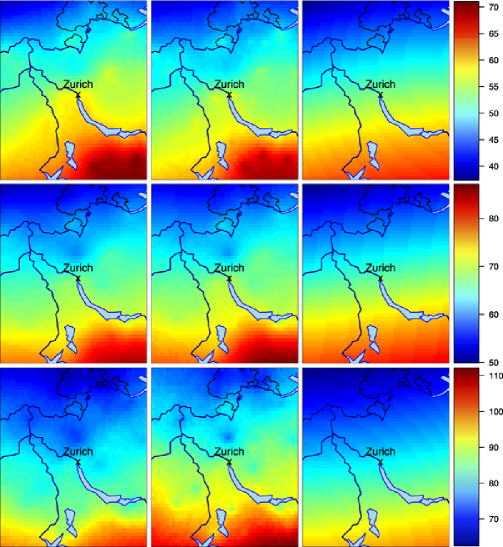
Figure 3: Maps of the (predictive) pointwise 25-year return level estimates for rainfall (mm) obtained from the latent variable and max-stable models. The top and bottom rows show the lower and upper bounds of the $95\%$ pointwise credible/confidence intervals. The middle row shows the predictive pointwise posterior mean and pointwise estimates. The left column corresponds to the latent variable model assuming ${\rm Gamma}(5,3)$ prior on $\lambda$. The middle column assumes the less informative priors $\lambda_{\eta}\sim{\rm Gamma}(1,100)$, $\lambda_{\tau}\sim{\rm Gamma}(1,10)$ and $\lambda_{\xi}\sim{\rm Gamma}(1,10)$. The right column corresponds to the extremal $t$ copula model.

Figure 3 shows maps of the predictive pointwise posterior mean for the $25$-year return level, with pointwise $95\%$ credible intervals. These maps were produced by first generating one conditional simulation of three independent Gaussian processes for each state of the Markov chain given its then-current values of $\bolds{\eta}$, $\bolds{\tau}$ and $\bolds{\xi}$, and then using this realization to compute pointwise $25$-year return levels at ungauged sites. This shows the main strength of the latent variable approach: the use of stochastic processes to model the spatial behavior of the marginal parameters enables us to capture complex local variation in the return levels that deterministic trend surfaces cannot reproduce. The simulation output can be manipulated to obtain posterior standard errors and other uncertainty measures for quantities of interest, such as these or other return levels.

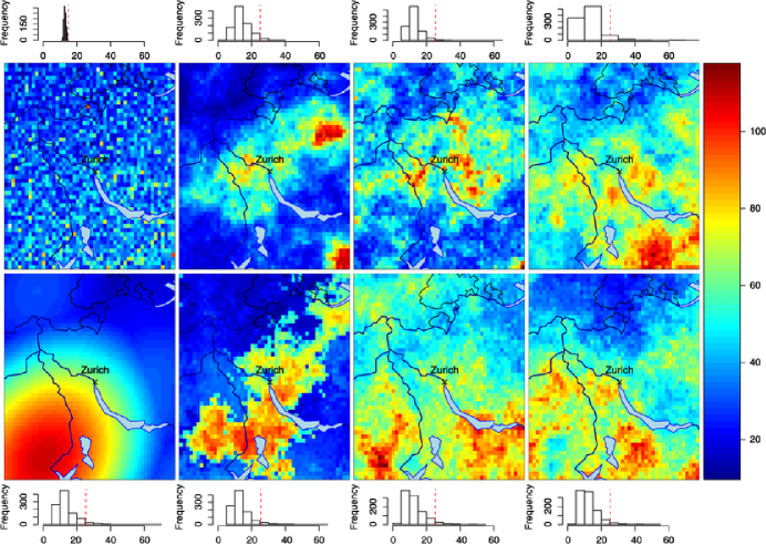
Figure 4: One realization from each of the models. From left to right, the top row shows results from the latent variable, Student $t$ copula, Hüsler–Reiss copula and extremal-$t$ copula models; the bottom row shows results from the Smith, Schlather, geometric Gaussian and Brown–Resnick models. The extreme top and bottom panels show histograms of 1000 realizations of the summary statistic $T$, and the vertical lines correspond to the realizations shown.

Although the pointwise return level maps look reasonable, the latent variable approach does not provide plausible spatial process realizations. The upper left panel of Figure 4 shows one realization of the spatial process from this model. Clearly, the assumption of conditional independence given the latent process leads to unrealistic spatial structure, and this has a severe impact when using this model to analyze the multivariate distribution of extremes for several sites, or for regional analysis. Compared to the other models, the conditional independence assumption underlying the latent variable modelleads to much less variation in quantities such as the statistic used to choose the simulations shown, that is, $T=|\mathcal{B}|^{-1}\int_{x\in\mathcal{B}}Z(x)$, where $\mathcal{B}$ denotes a ball of radius 10 km centered on Zurich.

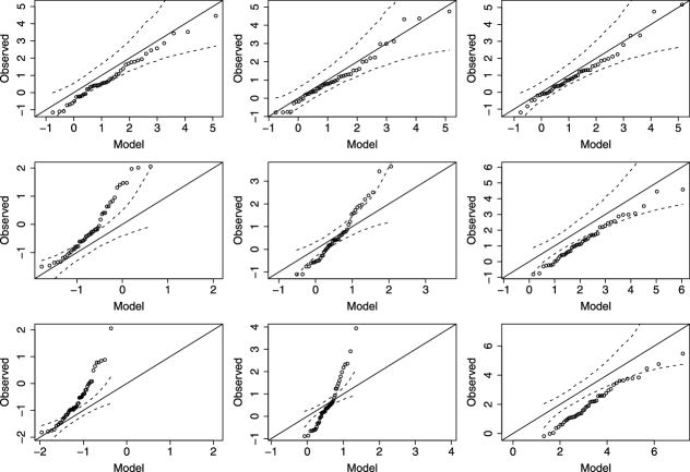
Figure 5: Model checking for the latent variable model. The top row compares pairwise maxima simulated from the model and the observed maxima for pairs of stations separated by 7 km (left), 45 km (middle) and 83 km (right). The middle row compares the observed and predicted minima (left), mean (middle) and maxima (right) for a group of five stations chosen randomly. The bottom row compares the observed and predicted minima (left), mean (middle) and maxima (right) for all 16 stations kept for model validation. Overall 95% confidence envelopes are also shown. For clarity the values are transformed to the unit Gumbel scale using the probability integral transform for the fitted GEV model for each station.

Figure 5 confirms this through QQ-plots for different groupwise maxima. The multivariate distribution of the validation sample is very poorly modeled, because the conditional independence assumption is not appropriate for extreme rainfall events involving dependence between stations. For instance, when groups of maxima are considered, the latent variable model seems to systematically overestimate their joint distribution, by an amount that depends on the number of sites contributing to the maximum.

7.3 Copula Models

In this section we describe the results obtained from fitting the copula models. We fit the nonextremal Gaussian and Student $t$ copulas using the full likelihood, and the extremal copulas using maximum pairwise likelihood estimation. In each case we use the marginal structures (24)–(26) and the correlation functions in Table 1.

We first fitted the Gaussian and Student $t$ copulas (14) and (5.2) with GEV marginal distributions and various correlation functions, using the corresponding likelihoods. These copulas are not max-stable, so we do not expect this approach to yield good models for the joint extremes; this is essentially a frequentist approach to fitting models like that of Sang and Gelfand (2010). The left panel of Figure 6 shows the empirical semivariogram for the fitting and validation stations, with the fitted semivariograms from the best and worst-fitting models obtained using this approach. The Student $t$ fit seems reasonable, though not ideal, but the center and right panels show that the corresponding extremal coefficients do not match to the data; the extremal coefficient for the Gaussian copula equals 2 at all distances $h$, and that for the Student $t$ copula predicts very weak extremal dependence inconsistent with the observed extremes.

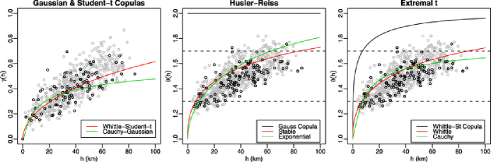
Figure 6: Comparison between data and fitted copula models. The left panel shows the empirical semivariogram values for the pairs of stations used in the fitting (grey) and the validation stations (black), with the fitted semivariograms for the best (red) and worst (green) models. The center and right panels show $F$-madogram estimates of the pairwise extremal coefficients for the fitting and validation stations, and the fitted extremal coefficient functions for the copula models with the lowest CLIC (red line) and the highest CLIC (green line). The horizontal dashed lines in the center and right panels are at 1.3 and 1.7; these panels also show the extremal coefficient curves (black) for the models in the left panel. The center and right panels also show the extremal coefficients corresponding to the best-fitting nonextremal Gaussian and Student $t$ copula models; that for the Gaussian model takes a constant value 2, and that for the $t$ model lies well above the empirical extremal coefficients.

Turning to extremal copulas, Table 4 shows that the extremal $t$ models all fit the data appreciably better than do the Hüsler–Reiss models, with well-determined but small estimates of the degrees of freedom. As in more standard geostatistical applications, it is difficult to estimate the scale and shape parameters of the correlation functions, and this is compounded by the presence of the degrees of freedom for the extremal $t$ models; the standard errors for $\lambda$ and $\kappa$ can be large and somewhat variable. At first sight the differences in the estimates of $\lambda$ in the upper and lower parts of the table are surprising, but they are clarified by noting that the limit (5.3) obtained by letting $\nu\to\infty$ in (5.3) implies that for large $\nu$, $(\|h\|/\lambda)^{\kappa}\approx 2\nu(\|h\|/\lambda^{\prime})^{\kappa^{\prime}}$, where the parameters $\lambda^{\prime},\kappa^{\prime}$ are those of the extremal $t$ model and those without the primes are those of the Hüsler–Reiss model. We therefore expect that $\kappa^{\prime}\approx\kappa$ and $\lambda^{\prime}\approx\lambda(2\nu)^{1/\kappa}$, and this is indeed the case, apart from estimation error. Perhaps not surprisingly for rainfall data, which tend to have high local variation corresponding to rough spatial processes, the estimates of the shape parameters $\kappa$ are less than unity.

To aid the comparison of these models, we introduce an extremal practical range. In conventional geostatistics with stationary isotropic correlation, the practical range is the distance $h$ for which the correlation function $\rho(h)=0.05$. In the extremal context we instead use the distances $h_{-}$ and $h_{+}$ satisfying $\theta(h_{-})=1.3$ and $\theta(h_{+})=1.7$. Table 4 suggests that these distances are more stable than the parameters of the correlation functions themselves, though those for the exponential and Cauchy functions, which provide the worst fits, indicate stronger dependence of extremal rainfall. Overall inclusion of the degrees of freedom has a large impact on the model fit, while the effect of varying the correlation function is more limited. The extremal $t$ model with the Whittle–Matérn correlation function provides the minimum CLIC, consistent with the best fit obtained with max-stable models below, from the geometric Gaussian process.

Table 4: Fits of extremal $t$ and Hüsler–Reiss copula models to Swiss rainfall data. The first column reports the correlation function used, and the second to fourth columns give parameter estimates (standard errors); DoF is the estimated degrees of freedom, $\lambda$ is the scale parameter and $\kappa$ is the shape parameter. $(\ast)$ denotes that the parameter is held fixed. $h_{-}$ and $h_{+}$ are the estimated distances at which $\theta(h)$ equals 1.3 and 1.7. NoP is the number of parameters, $\ell_{p}$ is the maximized composite log-likelihood, and CLIC is the information criterion

	Extremal $\bolds{t}$
Correlation	DoF	$\bolds{\lambda}$ (km)	$\bolds{\kappa}$	$\bolds{h_{-}}$ (km)	$\bolds{h_{+}}$ (km)	NoP	$\bolds{\ell_{p}}$	CLIC
Whittle	5.5 (2.1)	316 (235)0	0.39 (0.05)	6.9	087	10	$-$210,232	423,107
Stable	5.5 (2.1)	279 (206)0	0.81 (0.09)	6.9	088	10	$-$210,233	423,110
Exponential	4.8 (1.5)	160 (62)00	1.00 $(\ast)$0..	9.0	072	09	$-$210,264	423,131
Cauchy	5.5 (2.1)	00006.3 (1.2)00	0.06 (0.03)	7.6	217	10	$-$210,296	423,230
		Hüsler–Reiss
Semivariogram		$\bolds{\lambda}$ (km)	$\bolds{\kappa}$	$\bolds{h_{-}}$ (km)	$\bolds{h_{+}}$ (km)	NoP	$\bolds{\ell_{p}}$	CLIC
Stable		11.8 (3.4)	0.74 (0.07)	5.8	84	9	$-$210,348	423,232
Exponential		14.6 (3.2)	1.00 $(\ast)$.00	8.7	63	8	$-$210,438	423,338

The center and right panels of Figure 6 compare the $F$-madogram estimates of the extremal coefficients between pairs of stations with the extremal coefficient functions obtained with the fitted Hüsler–Reiss and extremal $t$ models that have the largest and smallest CLIC values. The interpretation of such plots is somewhat awkward because the $F$-madogram estimates do not correspond to independent pairs of stations, but both fits appear to underestimate extremal dependence at distances under 30 km, and to provide better fits, at least to the grey points, at longer distances.

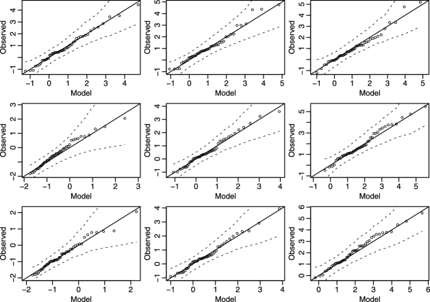
Figure 7: Model checking for the extremal $t$ model with the Whittle–Matérn correlation function. For details, see the caption to Figure 5.

The rightmost three top panels in Figure 4, which show one realization from each of the Student $t$ and best Hüsler–Reiss and extremal $t$ copula models, show that these processes provide more realistic spatial dependence than does the latent process, though the Student $t$ realization gives a smaller area with really large precipitation, consistent with Figure 6.

Figure 7 shows the outcome of the model checking procedure for extremal $t$ models with the Whittle–Matérn correlation function, using the validation stations. Overall the fit seems much better than for the latent variable model. For comparison, Figure 8 displays the results of the model checking procedure for the Student $t$ copula model with the Whittle–Matérn correlation function. Although the fit is appreciably better than for the latent variable model, the systematic appearance of the observed minima above the diagonal and of the observed maxima below the diagonal suggest that the model does not include enough dependence in the extremes, as one anticipates from the rapidly decreasing extremal dependence for this model, shown in the right panel of Figure 6. Overall the fit is not as good as that of the extremal $t$ copula, shown in Figure 7.

Figure 8: Model checking for the Student $t$ copula model with the Whittle–Matérn correlation function. For details, see the caption to Figure 5.

A map of the pointwise 25-year return levels for this model is very similar to the corresponding plot for the max-stable models, shown in Figure 3; both are less plausible than the corresponding map for the latent variable model, which shows better adaptation to local variation, though at the cost of more uncertainty for quantile estimates.

7.4 Max-Stable Models

In this section we focus on the max-stable models, again fitted with the marginal trend surfaces (24)–(26). Table 5 summarizes the fitted models. The Brown–Resnick and the geometric Gaussian models have the smallest CLIC values, perhaps owing to the behavior of their extremal coefficients for large distances. The variance parameter $\sigma^{2}$ in the geometric Gaussian model controls the upper bound of the extremal coefficient function, for instance, for an isotropic correlation function in $\mathbb{R}^{2}$ $\theta(h)\leq 2\Phi(0.838\sigma)$, for all $h\geq 0$. Hence, this model allows extremal coefficients $\theta(h)\approx 2$ if $\sigma^{2}$ is large enough. The Brown–Resnick model with variogram $\gamma(h)=|h|^{\alpha}$, $0<\alpha\leq 2$, also allows $\theta(h)\to 2$ when $h\to+\infty$, because then $\gamma(h)\to+\infty$. These differ from theSchlather model, which imposes $\theta(h)\to 1+1/2^{1/2}$ as $h\to\infty$. See Figure 9.

Table 5: Summary of the max-stable models fitted to the Swiss rainfall data. Standard errors are in parentheses. $(\ast)$ denotes that the parameter was held fixed. $h_{-}$ and $h_{+}$ are, respectively, the distances for which $\theta(h)$ is equal to $1.3$ and $1.7$. NoP is the number of parameters. $\ell_{p}$ is the maximized composite log-likelihood and CLIC is the corresponding information criterion

	Smith
Correlation	$\bolds{\sigma_{11}}$ (km)	$\bolds{\sigma_{12}}$ (km)	$\bolds{\sigma_{22}}$ (km)	$\bolds{h_{-}}$ (km)	$\bolds{h_{+}}$ (km)	NoP	$\bolds{\ell_{p}}$	CLIC
Isotropic	$259~{}(45)$	$\phantom{6}0~{}(\ast)$	$\sigma_{22}=\sigma_{11}$	$12.4$	$33$	0$8$	$-$212,455	427,113
Anisotropic	$251~{}(46)$	$64~{}(13)$	$290~{}(50)$	$6.6$–$11.1$	$18$–$30$	$10$	$-$212,395	427,020
	Schlather
Correlation		$\bolds{\lambda}$ (km)	$\bolds{\kappa}$	$\bolds{h_{-}}$ (km)	$\bolds{h_{+}}$ (km)	NoP	$\bolds{\ell_{p}}$	CLIC
Whittle		$39.3~{}(21.4)$	$0.44~{}(0.12)$	$6.0$	0$147$	$9$	$-$210,813	424,200
Stable		$34.8~{}(11.5)$	$0.95~{}(0.16)$	$6.3$	0$146$	$9$	$-$210,815	424,206
Exponential		$34.1~{}(9.0)$1	$1.00~{}(\ast)$00.	$6.8$	0$134$	$8$	$-$210,816	424,167
Cauchy		$\phantom{3}8.0~{}(2.2)$1	$0.34~{}(0.16)$	$7.1$	$2370$	$9$	$-$210,874	424,321
	Geometric Gaussian
Correlation	$\bolds{\sigma^{2}}$	$\bolds{\lambda}$ (km)	$\bolds{\kappa}$	$\bolds{h_{-}}$ (km)	$\bolds{h_{+}}$ (km)	NoP	$\bolds{\ell_{p}}$	CLIC
Whittle	$11.1~{}(3.8)$00	$700~{}(\ast)$00..	$0.37~{}(0.03)$	$5.8$	0$86$	$9$	$-$210,349	423,232
Stable	$15.0~{}(5.4)$00	$1000~{}(\ast)$000..	$0.76~{}(0.06)$	$5.9$	0$86$	$9$	$-$210,349	423,233
Exponential	0$2.42~{}(0.93)$	00$53.2~{}(18.4)$	$1.00~{}(\ast)$00.	$7.0$	$116$	$9$	$-$210,368	423,271
Cauchy	$30.9~{}(8.1)$00	000$5.2~{}(0.66)$	$0.01~{}(\ast)$00.	$6.7$	$192$	$9$	$-$210,412	423,355
	Brown–Resnick
Variogram		$\bolds{\lambda}$ (km)	$\bolds{\alpha}$	$\bolds{h_{-}}$ (km)	$\bolds{h_{+}}$ (km)	NoP	$\bolds{\ell_{p}}$	CLIC
Fractional		$30~{}(9.23)$	$0.74~{}(0.07)$	$5.8$	$84$	$9$	$-$210,348	423,231
Brownian		$29~{}(6.36)$	$1.00~{}(\ast)$00.	$8.7$	$63$	$8$	$-$210,438	423,338

Isotropic and anisotropic Smith models were also considered. Their CLIC values show that the anisotropic model is better, but both fit much less well than the other models. This might be explained by the lack of flexibility of this model, which assumes a deterministic shape for the storms and leads to dependence of the extremal coefficient on the Mahalanobis distance rather than on a more flexible function of distance; it corresponds to taking the Brown–Resnick model with variogram $\gamma(h)\propto h^{2}$.

Apart from the Smith models, all give comparable estimates for $h_{-}$, though the choice of the correlation function may have a large impact on the estimation of $h_{+}$. In particular, the Cauchy function differs greatly from the others. The best-fitting models show values for $h_{+}$ similar to those from the best extremal copula models, though the copula models have lower CLIC values.

The geometric Gaussian model with Whittle–Matérn or stable correlation functions and the Brown–Resnick model appear to provide the best fits to our data, though we had difficulties in simultaneously estimating $\sigma^{2}$, $\lambda$ and $\kappa$ for the former models. In accordance with our results for the latent variable model, these parameters seem not to be jointly identifiable (Zhang (2004)), perhaps because of the upper limit of around 90 km on the distances between sites, which means that ${\sigma}^{2}$ is difficult to estimate from these data. The safest strategy when using the geometric Gaussian model appears to be to fix one of these parameters, preferably the range $\lambda$ or shape $\kappa$, which do not determine an upper bound for the extremal coefficient. Some numerical experimentation shows that $\sigma^{2}$ and $\lambda$ are strongly related: completely different values of them can lead to indistinguishable extremal coefficient functions, at least for the distances seen in our data.

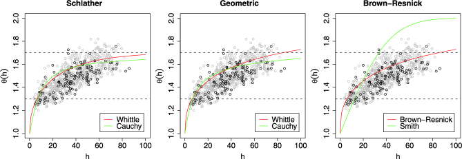
Figure 9: Comparison between the $F$-madogram estimates for the fitting (grey points) and the validation (black points) data sets and the estimated extremal coefficient functions for different max-stable models.

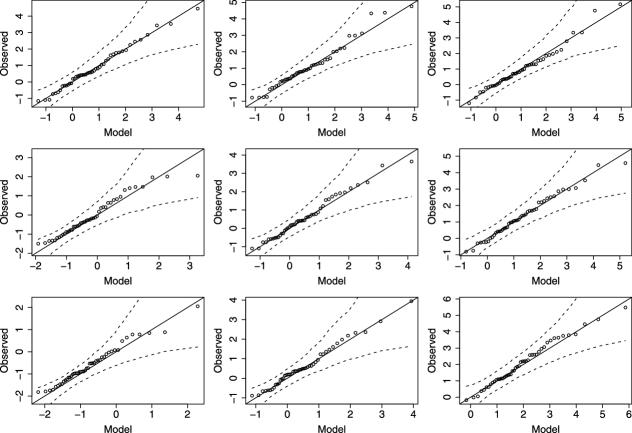
Figure 10: Model checking for the Brown–Resnick model. For details, see the caption to Figure 5.

Figure 10 shows the fits of the best max-stable model to the data from the validation stations. Pairwise dependencies seem to be well estimated whatever the distance between two sites, and the higher-dimensional properties also seem to be accurately modeled, even if different summary statistics are considered.

Figure 4, which plots one realization from the best Smith, Schlather, geometric Gaussian and Brown–Resnick max-stable models, illustrates the differences among them. The elliptical forms in the Smith model realization seem unrealistic, while the Schlather, geometric Gaussian and Brown–Resnick model realizations appear more plausible. The difference between those from the last three models is less obvious visually, though the geometric Gaussian and Brown–Resnick models tend to give less dependence at long ranges than does the Schlather model, owing to the restrictions that the latter imposes on the extremal coefficient.

The drawback of the max-stable process is that it may be difficult to find accurate trend surfaces for the marginal parameters. This may result in unrealistically smooth pointwise return levels, similar to that shown in Figure 3.

8 Discussion

If the purpose of spatial analysis of extremes is simply to map marginal return levels for the underlying process, a very simple approach is to apply kriging to quantiles estimated separately for each site. The strong asymmetry in the uncertainty suggests that this is best applied to transformed estimates, perhaps their logarithms, followed by back-transformation to the original scale. The obvious disadvantages of this approach are that maps for different quantiles may be contradictory, that their uncertainties may be hard to assess, and that the resulting maps may be inconsistent with risk assessment for more complex events.

Turning to the approaches discussed in detailabove, a major asset of latent variable models is flexibility: it is conceptually straightforward to add further elements or other layers of variation, if they are thought to be necessary, though the computations become more challenging. Moreover, the use of stochastic processes for the spatial distribution of the GEV parameters enables the treatment of situations for which these parameters display complex variation. Prediction at unobserved sites $x_{+}$ is also straightforward using conditional simulation of Gaussian random fields for each state of the chain, from which observations can be generated at each $x_{+}$, and it is straightforward to obtain measures of uncertainty for quantities of interest.

Apart from generic issues related to the choice of prior distribution in Bayesian inference, there are two main drawbacks to the latent variable approach in the present context. The first is that after the averaging over the underlying process $\{S(x)\}$, the marginal distribution of $\{Y(x)\}$ is not of extreme-value form, and therefore will not be max-stable. This contradicts the argument leading to (3), but might be regarded as the price to be paid for the flexibility of including latent variables and fully Bayesian inference; see, for example, Turkman, Turkman and Pereira (2010). The second drawback is more serious, and stems from the construction of the model: conditional on the underlying process, extremes will arise independently at adjacent sites. This is clearly unrealistic, and seems to undermine the use of this approach to forecasting for specific events, though it may still be very useful for the computation of marginal properties of extremal distributions, such as return levels. The copula-based approach of Sang and Gelfand (2010) is intended to deal with this, but results in Section 7.3 suggest that a closely-related frequentist copula model does not adequately explain the local extremal dependence of our annual maximum rainfall data, so the use of Gaussian copulas cannot be regarded as wholly satisfactory. A more promising approach has been suggested in the as-yet unpublished work of Reich and Shaby (2011), who develop a finite latent process approximation to the Smith process in a Bayesian framework, and are thus able to approximate this model closely using Markov chain Monte Carlo methods. They are also able to incorporate nonstationarity and latent process models for the marginal parameters.

Our rainfall application suggests that there is an awkward trade-off to be made in modeling spatial extremes. Latent variables allow a realistic and flexible spatial structure in the marginal distributions and thus enable a good assessment of the variation of return levels across space, but the spatial structure they attribute to extreme events seems quite unrealistic: compare the simulations in Figures 3 and 4. It would be worthwhile to investigate the fitting of such structures using pairwise likelihood, which is the only approach currently available for the fitting of the spatially appropriate copula and max-stable process models. Ribatet, Cooley and Davison (2012) report promising results from an investigation into the use of pairwise likelihood in Bayesian inference, but it would be good to have a better understanding of that approach.

The connections between copula and max-stable models also need more investigation: while the former seem to provide the best fits overall—compare Tables 4 and 5—the formulation of the latter in terms of a full spatial process is very attractive. Presumably the difference is simply a technical matter of using a spatially-defined dependence function and extending the copula models to the full spatial domain, but the connections are intriguing and merit further study.

Although we have used pairwise likelihood for inference, it would be worthwhile to investigate whether the inclusion of third- and higher-order marginal densities in the composite likelihood would increase its efficiency. Genton, Ma and Sang (2011) show that this increases the efficiency of estimation for the Smith model, but so far as we are aware, their work has not yet been extended to other max-stable models or used in applications. Another way to improve statistical efficiency while reducing the computational burden of the composite likelihood could be the downweighting or exclusion of likelihood contributions from sites very far apart, as suggested by Bevilacqua et al. (2012) and Padoan, Ribatet and Sisson (2010); in the context of time series, including unnecessary pairs can degrade inference (Davis and Yau (2011)), and simulations suggest that this is also true for certain models for spatial extremes (Gholamrezaee (2010); Padoan, Ribatet and Sisson (2010)). This is related to the issue of the scalability of the max-stable and extremal copula analyses: the combinatorial explosion associated with the use of pairwise likelihood might render these infeasible for data from thousands of sites. In such cases a judicious sub-sampling of pairs seems necessary, but our expectation is that inference should be feasible in such settings.

We apply our ideas to block maxima, essentially because this seems to be the only extremal setting for which spatial methods are currently available, but the extension to threshold modeling (Davison and Smith (1990); Coles and Tawn (1991)) would enable more flexible inference. Encouraging results for spatio-temporal modeling of rain data have been obtained in Huser and Davison (2012), and further exploration of related ideas, for example, due to Turkman, Turkman and Pereira (2010), seems eminently worthwhile.

Throughout the discussion above we have supposed that the classical theory of extremes provides appropriate models for maxima, and, in particular, that the extremal dependence observed in the data can be extrapolated to higher levels for which observations are unavailable. In practice, dependence is often seen to decrease for increasingly rare events, suggesting inadequacies in the classical formulation. The development of models for so-called near-independence (Ledford and Tawn, 1996, 1997; Heffernan and Tawn (2004); Ramos and Ledford (2009)) of spatial extremal data would be very valuable. Wadsworth and Tawn (2012) tackle this important topic.

Appendix: MCMC Algorithm for Latent Variable Model

Inference for our latent variable model may be performed using a Gibbs sampler, whose steps we now describe. Given a current value of the Markov chain

$$\psi_{t} = (\bolds{\eta}_{t},\bolds{\tau}_{t},\bolds{\xi}_{t},\alpha_{\eta,t},\lambda_{\eta,t},\alpha_{\tau,t},\lambda_{\tau,t},\alpha_{\xi,t},\lambda_{\xi,t},$$

$$\hskip 114.0pt{}\bolds{\beta}_{\eta,t},\bolds{\beta}_{\tau,t},\bolds{\beta}_{\xi,t}),$$

the next state $\psi_{t+1}$ of the chain is obtained as follows.

Step 1: Updating the GEV parameters at each site. Each component of $\bolds{\eta}_{t}=\{\eta_{t}(x_{1}),\ldots,\eta_{t}(x_{D})\}$ is updated singly according to the following scheme. Generate a proposal $\eta_{p}(x_{d})$ from a symmetric random walk and compute the acceptance probability

$$\alpha\{\eta_{t}(x_{d}),\eta_{p}(x_{d})\}$$

$$\quad=\min\bigl{\{}1,\pi\{y_{d}\mid\eta_{p}(x_{d}),\tau_{t}(x_{d}),\xi_{t}(x_{d})\}$$

$${}\hskip 29.0pt\qquad\times\pi(\bolds{\eta}_{p}\mid\alpha_{\eta},\lambda_{\eta},\bolds{\beta}_{\eta})$$

$$\qquad\big{/}\bigl{(}\pi\{y_{d}\mid\eta_{t}(x_{d}),\tau_{t}(x_{d}),\xi_{t}(x_{d})\}$$

$${}\hskip 72.0pt\qquad\times\pi(\bolds{\eta}_{t}\mid\alpha_{\eta},\lambda_{\eta},\bolds{\beta}_{\eta})\bigr{)}\bigr{\}},$$

that is, a ratio of GEV likelihoods times a ratio of multivariate Normal likelihoods. With probability $\alpha\{\eta_{t}(x_{d}),\eta_{p}(x_{d})\}$, the $\eta(x_{d})$ component of $\bolds{\psi}_{t+1}$ is set to $\eta_{p}(x_{d})$; otherwise it remains at $\eta_{t}(x_{d})$. The scale and shape parameters are updated similarly.

Step 2: Updating the regression parameters. Due to the use of conjugate priors, $\beta_{\eta}$ is drawn directly from a multivariate Normal distribution having covariance matrix and mean vector

$$\{(\Sigma_{\eta}^{*})^{-1}+\mathbf{X}_{\eta}^{\mathrm{T}}\Sigma_{\eta}^{-1}\mathbf{X}_{\eta}\}^{-1},$$

$$\{(\Sigma_{\eta}^{*})^{-1}+\mathbf{X}_{\eta}^{\mathrm{T}}\Sigma_{\eta}^{-1}\mathbf{X}_{\eta}\}^{-1}\{(\Sigma_{\eta}^{*})^{-1}\mu_{\eta}^{*}+\mathbf{X}_{\eta}^{\mathrm{T}}\Sigma_{\eta}^{-1}\bolds{\eta}\},$$

where $\mu_{\eta}^{*}$ and $\Sigma_{\eta}^{*}$ are the mean vector and covariance matrix of the prior distribution for $\bolds{\beta}_{\eta}$ and $\mathbf{X}_{\eta}$ is the design matrix related to the regression coefficients $\bolds{\beta}_{\eta}$. Again the regression parameters for the GEV scale and shape parameters are updated similarly.

Step 3: Updating the sill parameters of the covariance function. Due to the use of conjugate priors, $\alpha_{\eta}$ is drawn directly from an inverse Gamma distribution whose shape and rate parameters are

$$\tfrac{1}{2}{k}+\kappa_{\alpha}^{*},$$

$$\theta_{\alpha_{\eta}}^{*}+\tfrac{1}{2}{\alpha_{\eta,t}(\bolds{\eta}_{t}-\mathbf{X}_{\eta}\bolds\beta_{\eta,t})^{\mathrm{T}}\Sigma_{\eta,t}^{-1}(\bolds{\eta}_{t}-\mathbf{X}_{\eta}\beta_{\eta,t})},$$

where $\kappa_{\alpha_{\eta}}^{*}$ and $\theta_{\alpha_{\eta}}^{*}$ are respectively the shape and scale parameters of the inverse Gamma prior distribution and $\mathbf{X}_{\eta}$ is the design matrix related to the regression coefficients $\bolds{\beta}_{\eta}$. The sill parameters of the covariance function for the GEV scale and shape parameters are updated similarly.

Step 4: Updating the range parameters of the covariance function. Generate a proposal $\lambda_{\eta,p}\sim\break U(\lambda_{\eta,t}-\epsilon_{\lambda},\lambda_{\eta,t}+\epsilon_{\lambda})$ and compute the acceptance probability

$$\alpha(\lambda_{\eta,t},\lambda_{\eta,p})$$

$$\quad=\min\biggl{\{}1,{\pi(\bolds{\eta}_{t}\mid\alpha_{\eta,t},\lambda_{\eta,p},\bolds{\beta}_{\eta,p})\over\pi(\bolds{\eta}_{t}\mid\alpha_{\eta,t},\lambda_{\eta,t},\bolds{\beta}_{\eta,t})}$$

$$\hskip 32.0pt\qquad{}\times\biggl{(}{\lambda_{\eta,p}\over\lambda_{\eta,t}}\biggr{)}^{k_{\lambda_{\eta}}^{*}-1}\exp\biggl{(}{\lambda_{\eta,t}-\lambda_{\eta,p}\over\theta_{\lambda_{\eta}}^{*}}\biggr{)}\biggr{\}},$$

a ratio of multivariate Normal densities times the ratio of the prior densities and where $\kappa_{\lambda_{\eta}}^{*}$ and $\theta_{\lambda_{\eta}}^{*}$ are respectively the shape and the scale parameters of the Gamma prior distribution. With probability $\alpha(\lambda_{\eta,t},\lambda_{\eta,p})$, the $\lambda_{\eta}$ component of $\bolds{\psi}_{t+1}$ is set to $\lambda_{\eta,p}$; otherwise it remains at $\lambda_{\eta,t}$. The range parameters related to the scale and shape GEV parameters are updated similarly. If the covariance family has a shape parameter like the powered exponential or the Whittle–Matérn covariance functions, this is updated in the same way.

References

- Akaike (1973) {bincollection}[mr] \bauthor\bsnmAkaike, \bfnmH.\binitsH. (\byear1973). \btitleInformation theory and an extension of the maximum likelihood principle. In \bbooktitleSecond International Symposium on Information Theory (Tsahkadsor, 1971) (\beditor\bfnmB. N.\binitsB. N. \bsnmPetrov and \beditor\bfnmF.\binitsF \bsnmCzáki, eds.) \bpages267–281. \bpublisherAkadémiai Kiadó, \baddressBudapest. \bidmr=0483125 \bptokimsref \endbibitem
- Banerjee, Carlin and Gelfand (2004) {bbook}[auto:STB—2012/03/21—07:41:58] \bauthor\bsnmBanerjee, \bfnmS.\binitsS., \bauthor\bsnmCarlin, \bfnmB. P.\binitsB. P. and \bauthor\bsnmGelfand, \bfnmA. E.\binitsA. E. (\byear2004). \btitleHierarchical Modeling and Analysis for Spatial Data. \bpublisherChapman & Hall/CRC, \baddressNew York. \bptokimsref \endbibitem
- Beirlant et al. (2004) {bbook}[mr] \bauthor\bsnmBeirlant, \bfnmJan\binitsJ., \bauthor\bsnmGoegebeur, \bfnmYuri\binitsY., \bauthor\bsnmTeugels, \bfnmJozef\binitsJ. and \bauthor\bsnmSegers, \bfnmJohan\binitsJ. (\byear2004). \btitleStatistics of Extremes: Theory and Applications. \bpublisherWiley, \baddressChichester. \biddoi=10.1002/0470012382, mr=2108013 \bptokimsref \endbibitem
- Bevilacqua et al. (2012) {bmisc}[auto:STB—2012/03/21—07:41:58] \bauthor\bsnmBevilacqua, \bfnmM.\binitsM., \bauthor\bsnmGaetan, \bfnmC.\binitsC., \bauthor\bsnmMateu, \bfnmJ.\binitsJ. and \bauthor\bsnmPorcu, \bfnmE.\binitsE. (\byear2012). \bhowpublishedEstimating space and space–time covariance functions: A weighted composite likelihood approach. J. Amer. Statist. Assoc. 107. To appear. \bptokimsref \endbibitem
- Blanchet and Davison (2011) {barticle}[auto:STB—2012/03/21—07:41:58] \bauthor\bsnmBlanchet, \bfnmJ.\binitsJ. and \bauthor\bsnmDavison, \bfnmA. C.\binitsA. C. (\byear2011). \btitleSpatial modelling of extreme snow depth. \bjournalAnn. Appl. Stat. \bvolume5 \bpages1699–1725. \bptokimsref \endbibitem
- Boldi and Davison (2007) {barticle}[mr] \bauthor\bsnmBoldi, \bfnmM. O.\binitsM. O. and \bauthor\bsnmDavison, \bfnmA. C.\binitsA. C. (\byear2007). \btitleA mixture model for multivariate extremes. \bjournalJ. R. Stat. Soc. Ser. B Stat. Methodol. \bvolume69 \bpages217–229. \biddoi=10.1111/j.1467-9868.2007.00585.x, issn=1369-7412, mr=2325273 \bptokimsref \endbibitem
- Buishand, de Haan and Zhou (2008) {barticle}[mr] \bauthor\bsnmBuishand, \bfnmT. A.\binitsT. A., \bauthor\bparticlede \bsnmHaan, \bfnmL.\binitsL. and \bauthor\bsnmZhou, \bfnmC.\binitsC. (\byear2008). \btitleOn spatial extremes: With application to a rainfall problem. \bjournalAnn. Appl. Stat. \bvolume2 \bpages624–642. \biddoi=10.1214/08-AOAS159, issn=1932-6157, mr=2524349 \bptokimsref \endbibitem
- Butler et al. (2007) {barticle}[mr] \bauthor\bsnmButler, \bfnmAdam\binitsA., \bauthor\bsnmHeffernan, \bfnmJanet E.\binitsJ. E., \bauthor\bsnmTawn, \bfnmJonathan A.\binitsJ. A. and \bauthor\bsnmFlather, \bfnmRoger A.\binitsR. A. (\byear2007). \btitleTrend estimation in extremes of synthetic North Sea surges. \bjournalJ. Roy. Statist. Soc. Ser. C \bvolume56 \bpages395–414. \biddoi=10.1111/j.1467-9876.2007.00583.x, issn=0035-9254, mr=2409758 \bptokimsref \endbibitem
- Casson and Coles (1999) {barticle}[auto:STB—2012/03/21—07:41:58] \bauthor\bsnmCasson, \bfnmE.\binitsE. and \bauthor\bsnmColes, \bfnmS.\binitsS. (\byear1999). \btitleSpatial regression models for extremes. \bjournalExtremes \bvolume1 \bpages449–468. \bptokimsref \endbibitem
- Chavez-Demoulin and Davison (2005) {barticle}[mr] \bauthor\bsnmChavez-Demoulin, \bfnmV.\binitsV. and \bauthor\bsnmDavison, \bfnmA. C.\binitsA. C. (\byear2005). \btitleGeneralized additive modelling of sample extremes. \bjournalJ. Roy. Statist. Soc. Ser. C \bvolume54 \bpages207–222. \biddoi=10.1111/j.1467-9876.2005.00479.x, issn=0035-9254, mr=2134607 \bptokimsref \endbibitem
- Coles (2001) {bbook}[mr] \bauthor\bsnmColes, \bfnmStuart\binitsS. (\byear2001). \btitleAn Introduction to Statistical Modeling of Extreme Values. \bpublisherSpringer, \baddressLondon. \bidmr=1932132 \bptokimsref \endbibitem
- Coles and Casson (1998) {barticle}[auto:STB—2012/03/21—07:41:58] \bauthor\bsnmColes, \bfnmS. G.\binitsS. G. and \bauthor\bsnmCasson, \bfnmE.\binitsE. (\byear1998). \btitleExtreme value modelling of hurricane wind speeds. \bjournalStructural Safety \bvolume20 \bpages283–296. \bptokimsref \endbibitem
- Coles and Tawn (1991) {barticle}[mr] \bauthor\bsnmColes, \bfnmStuart G.\binitsS. G. and \bauthor\bsnmTawn, \bfnmJonathan A.\binitsJ. A. (\byear1991). \btitleModelling extreme multivariate events. \bjournalJ. Roy. Statist. Soc. Ser. B \bvolume53 \bpages377–392. \bidissn=0035-9246, mr=1108334 \bptokimsref \endbibitem
- Cooley and Sain (2010) {barticle}[mr] \bauthor\bsnmCooley, \bfnmDaniel\binitsD. and \bauthor\bsnmSain, \bfnmStephan R.\binitsS. R. (\byear2010). \btitleSpatial hierarchical modeling of precipitation extremes from a regional climate model. \bjournalJ. Agric. Biol. Environ. Stat. \bvolume15 \bpages381–402. \biddoi=10.1007/s13253-010-0023-9, issn=1085-7117, mr=2787265 \bptokimsref \endbibitem
- Cooley, Naveau and Poncet (2006) {bincollection}[mr] \bauthor\bsnmCooley, \bfnmDan\binitsD., \bauthor\bsnmNaveau, \bfnmPhilippe\binitsP. and \bauthor\bsnmPoncet, \bfnmPaul\binitsP. (\byear2006). \btitleVariograms for spatial max-stable random fields. In \bbooktitleDependence in Probability and Statistics. \bseriesLecture Notes in Statist. \bvolume187 \bpages373–390. \bpublisherSpringer, \baddressNew York. \biddoi=10.1007/0-387-36062-X_17, mr=2283264 \bptokimsref \endbibitem