Symmetric achromatic low-beta collider interaction region design concept

Abstract

We present a new symmetry-based concept for an achromatic low-beta collider interaction region design. A specially-designed symmetric Chromaticity Compensation Block (CCB) induces an angle spread in the passing beam such that it cancels the chromatic kick of the final focusing quadrupoles. Two such CCBs placed symmetrically around an interaction point allow simultaneous compensation of the 1st-order chromaticities and chromatic beam smear at the IP without inducing significant 2nd-order aberrations to the particle trajectory. We first develop an analytic description of this approach and explicitly formulate 2nd-order aberration compensation conditions at the interaction point. The concept is next applied to develop an interaction region design for the ion collider ring of an electron-ion collider. We numerically evaluate performance of the design in terms of momentum acceptance and dynamic aperture. The advantages of the new concept are illustrated by comparing it to the conventional distributed-sextupole chromaticity compensation scheme.

I Introduction

In order to achieve the highest possible luminosity in a collider des_rep12 ; erhic_zdr , the colliding beams must be focused to a small spot at the Interaction Point (IP). This tight focusing is unavoidably accompanied by a large transverse beam extension before the beam enters the Final Focusing Block (FFB). The size of the required beam extension is determined by the desired degree of beam squeezing at the IP and the focal length of the FFB, which is closely related to the space between the IP and the nearest focusing quadrupole. The larger this distance, the greater the beam extension must be. Since the FFB’s focal length depends on the particle’s momentum, the large beam size inside the FFB leads to a large correlation between the particle’s phase advance and its momentum handbook_ape .

The problem with such a correlation is two-fold. First of all, it induces a large chromatic betatron tune spread. Since the available betatron tune space is limited by the beam resonances, the chromatic betatron tune dependence limits the ring’s momentum aperture. Secondly, the chromatic dependence of the focal length causes chromatic beam smear at the IP, which can even dominate over the beam size due to the emittance, significantly increasing the beam spot size at the IP and resulting in luminosity loss. Thus, an Interaction Region (IR) design must employ sextupole magnets to compensate the chromatic effects nosochkov92 ; kekb_des_rep ; raimondi01 ; alexahin11 . However, the nonlinear sextupole fields generate 2nd- and higher-order aberrations to the particle trajectory at the IP, introduce nonlinear phase advance and limit the ring’s dynamic aperture. Compensation of these nonlinear effects is one of the main challenges of an IR and, even more generally, collider ring design. A commonly used chromaticity compensation technique is to install same-strength sextupoles in pairs with $-I$ (minus the identity) transformation between them to cancel their nonlinear kicks handbook_ape ; lee99 . However, this approach does not treat all of the sextupole-induced 2nd-order effects. Besides, organizing $-I$ transformations for the sufficient number of sextupole pairs for simultaneous compensation of the horizontal and vertical chromaticities is difficult. The concept described below not only includes all of the $-I$ transformation benefits but goes further by compensating all of the 2nd-order effects together with the 2nd-order beam smear at the IP. It also offers a more compact compensation scheme.

The IR design approach presented in this paper involves installation of a dedicated Chromaticity Compensation Block (CCB) next to the FFB derbenev07 ; wang09 ; morozov_ipac11 ; lin_ipac12 . In the CCB, certain symmetries of the beam orbital motion and dispersion are created using a symmetric arrangement of dipoles and quadrupoles. Two such CCBs are placed symmetrically around the IP. The symmetries of the beam orbital motion and dispersion combined with a symmetric quadrupole and sextupole arrangement in the CCBs then allow simultaneous compensation of the 1st-order chromaticities and chromatic beam smear at the IP without inducing significant 2nd-order aberrations and therefore helping preserve the ring’s dynamic aperture.

A schematic IR layout is shown in Fig. 1. The Beam Extension Section (BES) first expands the beam from its regular size in the arcs to the size required for final focusing. The beam next passes through the CCB, which creates in it an angle spread negatively correlated with the chromatic kick of the FFB, so that the FFB’s chromatic effect is cancelled. The FFB then focuses the beam to the required spot size at the IP. The IR design is mirror-symmetric with respect to the IP.

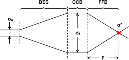
Figure 1: Schematic IR layout consisting of Beam Extension Section (BES), Chromaticity Compensation Block (CCB), and Final Focusing Block (FFB).

II Analytic description

In general, compensation of chromatic effects of a focusing lattice requires introduction of dipole and sextupole magnets along the lattice. The dipole field changes the beam reference orbit and creates dispersion, i.e. orbit dependence on the particle energy. The sextupole field then introduces an additional energy-dependent focusing strength to counter the original chromatic effect of the quadrupoles.

The particle motion in the horizontal $x$ and vertical $y$ planes about the reference orbit is described by the following equations courant58 :

$$\begin{split}&x^{\prime\prime}+(K^{2}-n)x=K\delta+f_{x},\\ &y^{\prime\prime}+ny=f_{y},\end{split}$$ (1)

where the prime ^′ denotes a derivative with respect to the longitudinal coordinate $s$, $K\equiv 1/\rho$ is the curvature of the bent reference orbit, $n\equiv(\partial B_{y}/\partial x)/(p/|e|)$ is the normalized quadrupole strength, and $\delta\equiv\Delta p/p$ is the particle’s relative momentum deviation from the reference value. The force terms $f_{x}$ and $f_{y}$ in Eq. (1) up to the 2nd order in $\delta$, $x$, and $y$ are given by

$$\begin{split}&f_{x}=-n\delta x+n_{s}(x^{2}-y^{2}),\\ &f_{y}=n\delta y-2n_{s}xy,\end{split}$$ (2)

where $n_{s}\equiv(\partial^{2}B_{y}/\partial x^{2})/(p/|e|)$ is the normalized sextupole strength. The quantities $K$, $n$, $n_{s}$, and, therefore, $f_{x}$ and $f_{y}$ are functions of $s$.

The particle trajectory in the horizontal plane can be represented as a superposition of the dispersive component $D\delta$ and the betatron component $x_{b}$:

$$x=D\delta+x_{b},$$ (3)

where the dispersion function $D\equiv\partial x/\partial\delta$ satisfies the equation

$$D^{\prime\prime}+(K^{2}-n)D=K.$$ (4)

Then the evolution of the betatron component is determined by the following equations:

$$\begin{split}x_{b}^{\prime\prime}&+(K^{2}-n)x_{b}=f_{x}=-(n-2Dn_{s})\delta x_{b}\\ &+D(Dn_{s}-n)\delta^{2}+n_{s}(x_{b}^{2}-y^{2}),\\ y^{\prime\prime}&+ny=f_{y}=(n-2Dn_{s})\delta y-2n_{s}x_{b}y.\end{split}$$ (5)

Sextupoles are usually placed in the ring arcs to compensate the energy dependence of the global betatron tunes. In that case, the chromaticity compensating sextupoles need to be configured to satisfy only two conditions associated with the $\delta x_{b}$ and $\delta y$ terms on the right hand side of Eq. (5), i.e. the integral effect of these terms over one revolution must be zero. The influence of the other three terms in Eq. (5) on the particle amplitude and global phase advance is zero when averaged over many revolutions. However, local chromatic effects in short sections or even at specific points like the IP where the beam experiences a strong transverse compression are generally not compensated on average in one turn. Compensation of these effects is a much more complicated problem, which requires taking into account all terms in Eq. (5). As one can see from these equations, the sextupole field component and dispersion give rise to the undesirable quadratic aberrations:

$$\begin{split}&\Delta x^{\prime\prime}\propto n_{s}[(D\delta)^{2}+x_{b}^{2}-y^{2}]-Dn\delta^{2},\\ &\Delta y^{\prime\prime}\propto-2n_{s}x_{b}y.\end{split}$$ (6)

Compensating the impact of these terms on the beam size at the IP, where the beam size is supposed to be extremely small, requires satisfying five different conditions in total. In order to explicitly state these conditions, we use the analytic perturbation approach below.

We represent the betatron motion as

$$\begin{split}x_{b}&=x_{1}+\tilde{x},\\ y&=y_{1}+\tilde{y}.\end{split}$$ (7)

where the unperturbed linear parts $x_{1}$ and $y_{1}$ satisfy the homogeneous equations:

$$\begin{split}&x_{1}^{\prime\prime}+(K^{2}-n)x_{1}=0,\\ &y_{1}^{\prime\prime}+ny_{1}=0,\end{split}$$ (8)

while the perturbed trajectory components are given by

$$\begin{split}&\tilde{x}^{\prime\prime}+(K^{2}-n)\tilde{x}=f_{x},\\ &\tilde{y}^{\prime\prime}+n\tilde{y}=f_{y}.\end{split}$$ (9)

We next express $x_{1}$ and $y_{1}$ as linear combinations of the two linearly-independent solutions $u(s)$ and $v(s)$ of Eq. (8):

$$\begin{split}x_{1}&=a_{x}u_{x}(s)+b_{x}v_{x}(s),\\ y_{1}&=a_{y}u_{y}(s)+b_{y}v_{y}(s).\end{split}$$ (10)

We then use the parameter variation technique to solve for the perturbed part

$$\begin{split}\tilde{x}&=\tilde{a}_{x}(s)u_{x}(s)+\tilde{b}_{x}(s)v_{x}(s),\\ \tilde{y}&=\tilde{a}_{y}(s)u_{y}(s)+\tilde{b}_{y}(s)v_{y}(s).\end{split}$$ (11)

Using the Cramer’s rule, the formal solution for the perturbed part can be written as

$$\begin{split}\tilde{x}(s)&=\frac{1}{W_{x}}[v_{x}\int_{0}^{s}u_{x}f_{x}ds-u_{x}\int_{0}^{s}v_{x}f_{x}ds],\\ \tilde{y}(s)&=\frac{1}{W_{y}}[v_{y}\int_{0}^{s}u_{y}f_{y}ds-u_{y}\int_{0}^{s}v_{y}f_{y}ds],\end{split}$$ (12)

where $W_{x}\equiv u_{x}v_{x}^{\prime}-u_{x}^{\prime}v_{x}$ and $W_{y}$ are the Wronskians of the $x$ and $y$ basis functions $u$ and $v$.

Suppose that $u$ and $v$ are chosen such that at the IP $u^{\ast}=0$ and $v^{\prime\ast}=0$, then the perturbed trajectory components at the IP are given by

$$\begin{split}\tilde{x}^{\ast}&=\frac{1}{W_{x}}v_{x}^{\ast}\int_{0}^{\ast}u_{x}f_{x}ds=-\frac{1}{u_{x}^{\prime\ast}}\int_{0}^{\ast}u_{x}f_{x}ds,\\ \tilde{y}^{\ast}&=\frac{1}{W_{y}}v_{y}^{\ast}\int_{0}^{\ast}u_{y}f_{y}ds=-\frac{1}{u_{y}^{\prime\ast}}\int_{0}^{\ast}u_{y}f_{y}ds.\end{split}$$ (13)

By performing the integration in Eq. (13) over the whole beam path from the start of the beam extension after the arc to the IP, we obtain the perturbation of the particle transverse position at the IP caused by the aberrations from all of the involved bends, quadrupoles, and sextupoles.

To find the next order correction to the unperturbed solution $x_{1}$ and $y_{1}$, in accordance with the iteration method, we plug the 1st-order unperturbed solution $x=D\delta+x_{1}$ and $y=y_{1}$ into the right-hand side of Eq. (9), obtaining the following equations for the 2nd-order correction:

$$\begin{split}\tilde{x}_{2}^{\prime\prime}&-n\tilde{x}_{2}=-(n-2Dn_{s})\delta x_{1}\\ &+D(Dn_{s}-n)\delta^{2}+n_{s}(x_{1}^{2}-y_{1}^{2}),\\ \tilde{y}_{2}^{\prime\prime}&+n\tilde{y}_{2}=(n-2Dn_{s})\delta y_{1}-2n_{s}x_{1}y_{1},\end{split}$$ (14)

where we neglected the term $K^{2}x$ on the left-hand side of the $x$ equation, since the effect of the orbit curvature on beam focusing at high energy is very small compared to that of the quadrupole field. Using Eq. (13), the 2nd-order correction to the particle’s unperturbed trajectory at the IP is given by

$$\begin{split}\tilde{x}_{2}^{\ast}=&-\frac{1}{u_{x}^{\prime\ast}}\int_{0}^{\ast}u_{x}[-(n-2Dn_{s})\delta x_{1}\\ &+D(Dn_{s}-n)\delta^{2}+n_{s}(x_{1}^{2}-y_{1}^{2})]ds,\\ \tilde{y}_{2}^{\ast}=&-\frac{1}{u_{y}^{\prime\ast}}\int_{0}^{\ast}u_{y}[(n-2Dn_{s})\delta y_{1}-2n_{s}x_{1}y_{1}]ds.\end{split}$$ (15)

Consider an almost parallel beam after the beam extension. The function $u$ then describes the dominant (“cos”-like) parallel component of the trajectory while the orthogonal solution $v$ is associated with the small remaining angular spread (“sin”-like trajectory). Then, neglecting the angular divergence, one can use Eq. (10) to approximate $x_{1}$ and $y_{1}$ in Eq. (15) as

$$\begin{split}x_{1}&\approx a_{x}u_{x}(s),\\ y_{1}&\approx a_{y}u_{y}(s),\end{split}$$ (16)

obtaining for the 2nd-order trajectory correction at the IP

$$\begin{split}\tilde{x}_{2}^{\ast}\approx&-\frac{1}{u_{x}^{\prime\ast}}\int_{0}^{\ast}u_{x}[-(n-2Dn_{s})\delta a_{x}u_{x}\\ &+D(Dn_{s}-n)\delta^{2}+n_{s}(a_{x}^{2}u_{x}^{2}-a_{y}^{2}u_{y}^{2})]ds,\\ \tilde{y}_{2}^{\ast}\approx&-\frac{1}{u_{y}^{\prime\ast}}\int_{0}^{\ast}u_{y}[(n-2Dn_{s})\delta a_{y}u_{y}\\ &-2n_{s}a_{x}u_{x}a_{y}u_{y}]ds.\end{split}$$ (17)

Clearly, aberration compensation requires

$$\begin{split}\tilde{x}_{2}^{\ast}=0,\\ \tilde{y}_{2}^{\ast}=0.\end{split}$$ (18)

Equation (17) then leads to the following five compensation conditions:

$$\begin{split}&(1)\hskip 14.22636pt2\int_{0}^{\ast}Dn_{s}u_{x}^{2}ds=\int_{0}^{\ast}nu_{x}^{2}ds,\\ &(2)\hskip 14.22636pt2\int_{0}^{\ast}Dn_{s}u_{y}^{2}ds=\int_{0}^{\ast}nu_{y}^{2}ds,\\ &(3)\hskip 14.22636pt\int_{0}^{\ast}D(Dn_{s}-n)u_{x}ds=0,\\ &(4)\hskip 14.22636pt\int_{0}^{\ast}n_{s}u_{x}^{3}ds=0,\\ &(5)\hskip 14.22636pt\int_{0}^{\ast}n_{s}u_{x}u_{y}^{2}ds=0.\end{split}$$ (19)

Conditions (1) and (2) in Eq. (19) are the usual conditions for compensation of the chromatic spread. Conditions (3)-(5) are the requirements for compensation of the 2nd-order dispersion effect and sextupole beam smear.

In the above analysis of the perturbed trajectory component, we so far ignored contribution of the angular spread, which is associated with the solution $v$. Even though this contribution is small compared to that of $u$, it may become dominant after compensation of the main aberration terms. Perhaps more importantly, the nonlinear phase advance associated with the angular spread may adversely affect the dynamic aperture. Using Eqs. (10) and (15) and neglecting the terms of the 2nd order in $v$, contribution of the angular spread to the 2nd-order perturbation at the IP can be written as

$$\begin{split}\Delta\tilde{x}_{2}^{\ast}\approx&-\frac{1}{u_{x}^{\prime\ast}}\int_{0}^{\ast}u_{x}[-(n-2Dn_{s})\delta b_{x}v_{x}\\ &+2n_{s}(a_{x}u_{x}b_{x}v_{x}-a_{y}u_{y}b_{y}v_{y})]ds,\\ \Delta\tilde{y}_{2}^{\ast}\approx&-\frac{1}{u_{y}^{\prime\ast}}\int_{0}^{\ast}u_{y}[(n-2Dn_{s})\delta b_{y}v_{y}\\ &-2n_{s}(a_{x}u_{x}b_{y}v_{y}+a_{y}u_{y}b_{x}v_{x})]ds.\end{split}$$ (20)

Compensation of the aberration terms in Eq. (20) imposes five more constraints in addition to those in Eq. (19):

$$\begin{split}&(1)\hskip 14.22636pt2\int_{0}^{\ast}Dn_{s}u_{x}v_{x}ds=\int_{0}^{\ast}nu_{x}v_{x}ds,\\ &(2)\hskip 14.22636pt2\int_{0}^{\ast}Dn_{s}u_{y}v_{y}ds=\int_{0}^{\ast}nu_{y}v_{y}ds,\\ &(3)\hskip 14.22636pt\int_{0}^{\ast}n_{s}u_{x}^{2}v_{x}ds=0,\\ &(4)\hskip 14.22636pt\int_{0}^{\ast}n_{s}u_{x}u_{y}v_{y}ds=0,\\ &(5)\hskip 14.22636pt\int_{0}^{\ast}n_{s}u_{y}^{2}v_{x}ds=0.\end{split}$$ (21)

Corrections beyond the 2nd order can be obtained by considering further iterations:

$$\begin{split}\tilde{x}&=\tilde{x}_{2}+\tilde{x}_{3}+\ldots,\\ \tilde{y}&=\tilde{y}_{2}+\tilde{y}_{3}+\ldots\end{split}$$ (22)

Thus, the 3rd-order correction terms can be found by integrating the following equations:

$$\begin{split}\tilde{x}_{3}^{\prime\prime}&-n\tilde{x}_{3}\approx n\delta^{2}x_{1}+(2Dn_{s}-n)\delta\tilde{x}_{2}\\ &+2n_{s}(x_{1}\tilde{x}_{2}-y_{1}\tilde{y}_{2})-\frac{1}{6}n^{\prime\prime}(D\delta+x_{1})^{3}\\ &+n_{o}[(D\delta+x_{1})^{3}-3(D\delta+x_{1})y_{1}^{2}],\\ \tilde{y}_{3}^{\prime\prime}&+n\tilde{y}_{3}\approx-n\delta^{2}y_{1}-(2Dn_{s}-n)\delta\tilde{y}_{2}\\ &-2n_{s}(x_{1}\tilde{y}_{2}+y_{1}\tilde{x}_{2})+\frac{1}{6}n^{\prime\prime}y_{1}^{3}\\ &+n_{o}[y_{1}^{3}-3(D\delta+x_{1})^{2}y_{1}],\end{split}$$ (23)

where we introduced the octupole field component $n_{o}\equiv(\partial^{3}B_{y}/\partial x^{3})/(p/|e|)$. The higher-order terms should be studied to determine their effects on the beam smear at the IP and the ring’s dynamic aperture. Equation (23) can be integrated similarly to Eq. (14); however, a complete analytic analysis clearly becomes rather cumbersome even in this 3rd-order case and one must employ a numerical approach. Nevertheless, one can still use Eq. (23) to identify the symmetries helpful in compensating the higher-order aberrations to guide the numerical studies.

III IR linear optics design

Equation (19) is an analytic representation of the interaction region design requirements up to the 2nd order in effects on the particle trajectory. By imposing certain symmetries of the orbital motion, dispersion and magnetic field components with respect to the center of the CCB, namely,

$$\begin{split}&u_{x}(s)=\mp u_{x}(-s),\\ &u_{y}^{2}(s)=u_{y}^{2}(-s),\\ &D(s)=\pm D(-s),\\ &n(s)=n(-s),\\ &n_{s}(s)=\pm n_{s}(-s),\end{split}$$ (24)

the five conditions of Eq. (19) are reduced to just the first two, i.e. the linear chromaticity compensation conditions. While creating chromatic kick, the CCB does not generate the nonlinear aberrations associated with the 2nd-order effects of the dispersion and transverse beam sizes in the sextupole fields. All these terms corresponding to conditions (3)-(5) of Eq. (19) are automatically compensated inside the CCB due to the special optics design and lattice symmetry. Equation (19) ignores the effect of the beam angular spread, which is admittedly small since the beam is assumed to be greatly extended and almost parallel at the entrance into the CCB. However, this effect may adversely affect the ring’s dynamic aperture. The 2nd-order terms associated with the beam’s angular spread are given by Eq. (21). The symmetry conditions in Eq. (24) do not give any advantage in this case. The significance of these and higher-order terms needs to be examined in each specific case and any required compensation may be done by introducing additional sextupole and higher-order multipole families, perhaps, also with appropriate types of symmetry.

We next test our symmetry concept by developing a conceptual IR design morozov_ipac11 ; lin_ipac12 for the ion collider ring of the Medium-energy Electron-Ion Collider (MEIC) that is being proposed by Jefferson Lab des_rep12 . Note that this is a proof-of-principle demonstration rather than a final IR design. It is used primarily to validate our symmetry-based chromaticity compensation concept. However, due to the modularity of our approach and the fact that the concept is independent of a particular FFB design, the IR design presented in this paper can be easily optimized to meet any specific nuclear physics detector requirements as discussed in des_rep12 ; morozov_ipac12 .

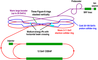
Figure 2: Schematic layout of the proposed MEIC complex.

Figure 2 shows a proposed layout of the MEIC complex des_rep12 . The main MEIC parameters are summarized in Table 1. As shown in Fig. 2, the electron and ion collider rings have geometrically-matching figure-8 shapes consisting of two $240^{\circ}$ arcs connected by two straight sections crossing each other in the middle at $60^{\circ}$. There is a total of two IPs: one IP per straight. The rings are stacked vertically in the arcs but, at the IPs, the beams cross in the horizontal plane. This is done by keeping the electron ring flat and bringing the ion beam to the electron beam’s plane using vertical chicanes located at the ends of the arcs.

Table 1: Main MEIC parameters.

Parameter	Unit	Electrons	Protons
Momentum range	GeV/$c$	3-11	20-100
Optimization point	GeV/$c$	5	60
Polarization	%	$\sim 80$	$>70$
Collision frequency	MHz	748.5
Particles per bunch	$10^{10}$	2.5	0.42
Beam current	A	3.0	0.5
$\Delta p/p$ (rms)	$10^{-3}$	0.7	0.3
Bunch length (rms)	mm	7.5	10
Norm. $x$ emit. (rms)	$\mu$m	54	0.35
Norm. $y$ emit. (rms)	$\mu$m	11	0.07
$\beta_{x}$ at IP $(\beta_{x}^{*})$	cm	10
$\beta_{y}$ at IP $(\beta_{y}^{*})$	cm	2
Collider ring length	m	1340
Luminosity per IP	cm-2s-1	$5.6\times 10^{33}$

Since the IR design concepts are similar for the two collider rings, below we focus our discussion on the ion collider ring, which is perhaps more challenging due to its larger natural linear chromaticities des_rep12 . Two IRs are incorporated into the ion ring’s two straight sections. The IR sections are assumed identical and the ring is arranged in a two-fold symmetric way. The ring’s horizontal $\nu_{x}$ and vertical $\nu_{y}$ betatron tunes are set to 23.273 and 21.285, respectively, by adjusting the phase advance outside of the IRs. The ring lattice used in the below simulations is fairly basic; it does not include components such as RF cavities, detector solenoids, vertical chicanes, spin control devices, injection/extraction elements, etc. However, the details of the ring design outside of the IR sections have little impact on the results of this paper and their description can be found in des_rep12 . Therefore, below we focus our attention on the IR design.

A conceptual drawing of an IR with a CCB that has an even symmetry of the dispersion and an odd symmetry of the horizontal betatron trajectory is shown in Fig. 3. If one then uses an even symmetry of the sextupole fields, conditions (3)-(5) of Eq. (19) are automatically satisfied. The two remaining chromaticity compensation conditions are satisfied by adjusting the fields of, at least, two sextupole families. This can be attained using the difference in the behavior of the horizontal and vertical $\beta$-functions.

In Fig. 3, there are two identical bends at the beginning and at the end of the CCB, which generate and then suppress the dispersion while symmetric quadrupole optics ensures the appropriate symmetries of the betatron and dispersive orbital components with respect to the center of the CCB. When designing the ion interaction region of an electron-ion collider, one has to keep in mind that it has to match the footprint of the electron interaction region. In the electron ring, since the CCB dipoles are located in regions with large $\beta$-function values, their maximum bends must be limited to avoid their emittance-degrading impact. In the ion ring, on the other hand, it is advantageous to have strong bends to produce a large dispersion thus reducing required sextupole fields and their nonlinear effects. These bend requirements are somewhat contradicting. Our solution is to use alternating but still symmetric bends in the ion CCB. One can then generate a large dispersion while having the flexibility of the footprint geometry.

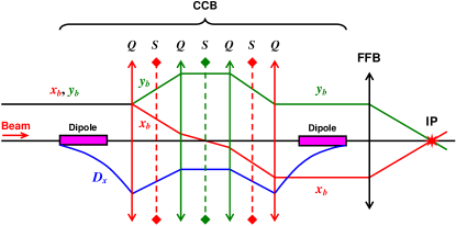
Figure 3: A conceptual drawing of an IR with a CCB that has an odd-symmetry horizontal betatron trajectory $x_{b}$, an even-symmetry vertical betatron trajectory $y_{b}$, and an even-symmetry horizontal dispersion $D_{x}$. It shows a possible arrangement of dipoles, quadrupoles $Q$, and sextupoles $S$ that satisfies the magnetic field symmetry requirements and produces the desired symmetries of $x_{b}$, $y_{b}$, and $D_{x}$.

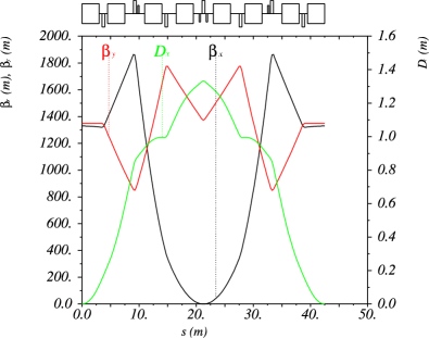
Figure 4: CCB optics.

Since the chromaticity correction scheme is independent of particular BES and FFB implementations, we first focus on the CCB design. Figure 4 shows CCB optics developed for the MEIC ion collider ring following the concept illustrated in Fig. 3. Note that, in comparison to the simplified schematic of Fig. 3, a larger number of quadrupoles were used to better control the beta function behavior. The CCB is composed of eight symmetrically-arranged alternating bends with seven quadrupoles placed symmetrically between them. The sum of the absolute values of all dipole bending angles is 480 mrad, while, due to the alternation of their bending directions, the net CCB bending angle is 120 mrad. The quadrupole strengths are adjusted to produce a total CCB transfer matrix that meets the symmetry requirements of Eq. (24).

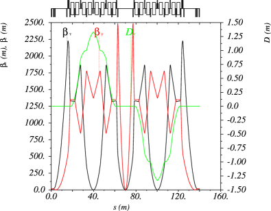
Figure 5: Complete IR optics of the MEIC ion collider ring. The IP is located at the symmetry point in the middle.

For the conceptual study presented in this paper, a simple quadrupole doublet is used for the FFB. As shown in Table 1, the design values of the horizontal and vertical $\beta$-functions at the IP $(\beta_{x,y}^{*})$ are 10 and 2 cm, respectively. The distance from the IP to the front face of the nearest FFB quadrupole is assumed to be 7 m, which, in combinations with the $\beta_{x,y}^{*}$ values, determines the maximum values of the $\beta$-functions in the IR region. The FFB optics design also determines the Twiss function values at the entrance into the CCB. The FFB quadrupole strengths, lengths and spacing are adjusted so that the $\beta$-functions have roughly equal values at the entrance into the CCB and the $\alpha$-functions $(\alpha_{x,y}\equiv-(\partial\beta_{x,y}/\partial s)/2)$ are equal to zero in the middle of the CCB. A BES consisting of 7 quadrupoles then matches the CCB optics to the ring’s regular lattice. This involves a substantial beam extension and therefore requires an appropriately large amount of longitudinal space. The IR is arranged symmetrically with respect to the IP. The complete IR optics of the MEIC ion collider ring is shown in Fig. 5. The detector solenoid and its coupling compensation elements are not included in this design. Note that the CCB bends on the opposite sides of the IP are reversed making the dispersion anti-symmetric with respect to the IP. This is also done for the purpose of electron and ion IR footprint matching.

The optics shown in Figs. 4 and 5 corresponds to the collider mode of operation. Since the injected beam’s emittance is typically much greater than after acceleration and cooling, keeping the collider-mode optics at injection may result in an unacceptably large beam size. Therefore, to keep the magnet apertures reasonable, the maximum $\beta$-functions occurring in the IR section may need to be reduced at injection and during acceleration and then restored for the collider operation. The described IR design allows a straightforward implementation of such a “$\beta$ squeeze”. Since entering and exiting the CCB the dispersion is suppressed and the $\alpha$-functions are almost zero, the CCB optics is compatible with any initial $\beta$-functions without any adjustment required as long as $\alpha_{x,y}$ have appropriate close-to-zero values. Thus, the size of the $\beta$-functions inside the IR can be controlled by adjusting the $\beta$-function values at the end of the BES. This requires only changing the optics of the BES with the rest of the ring optics intact.

IV Momentum acceptance and dynamic aperture

IV.1 Chromaticity compensation and momentum acceptance

In accordance with our chromaticity compensation concept, two sextupole pairs are inserted in each CCB. The sextupoles in each pair are identical and are placed symmetrically with respect to the center of the CCB. The sextupoles are shown in Figs. 4 and 5 by the shorter bars. The sextupole positions are chosen at the points where the dispersion is near maximum and there is a large difference between the horizontal and vertical $\beta$-functions. The two parameters corresponding to the strengths of the sextupole pairs are adjusted to compensate the horizontal $\xi_{x}$ and vertical $\xi_{y}$ natural linear chromaticities.

In this collider ring design des_rep12 , the total values of $\xi_{x}$ and $\xi_{y}$ are -278 and -268, respectively. Contributions of the IRs to $\xi_{x}$ and $\xi_{y}$ are -254 (91.4%) and 245 (91.3%), respectively. Therefore, contribution of the remainder of the ring is almost negligible and can also be compensated locally by the CCBs. The two sextupole families are used to adjust the slopes of the chromatic horizontal and vertical betatron tune curves to zero. The chromatic tune dependence before and after the compensation is shown in Fig. 6. The horizontal and vertical tune variations are less than 0.02 and 0.03, respectively, within $\Delta p/p$ of about $\pm 4\times 10^{-3}$.

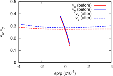
Figure 6: Momentum dependence of the horizontal $\nu_{x}$ (red) and vertical $\nu_{y}$ (blue) fractional betatron tunes before (solid lines) and after (dashed lines) the linear chromaticity compensation.

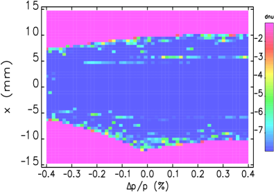
Figure 7: Frequency map in the $(x-\Delta p/p)$ phase space. The color reflects the tune change in terms of the tune diffusion $d$ defined as $d\equiv\log(\Delta\nu_{x}^{2}+\Delta\nu_{y}^{2})$.

An effective method to evaluate the nonlinearity of a particle’s dynamics is to obtain a frequency map laskar95 from particle tracking. At the design 60 GeV/$c$ proton beam momentum of the MEIC ion collider ring, the maximum horizontal and vertical rms beam sizes are 3.2 and 1.6 mm, respectively, due to a relatively large detector space of $\pm 7$ m. This makes it more challenging to obtain a sufficiently large dynamic aperture in the horizontal dimension. Therefore, the frequency map is first computed in the $(x-\Delta p/p)$ phase space as shown in Fig. 7. The map is obtained by tracking particles for 2000 turns using a well-established accelerator simulation software Elegant borland_elegant . All ring components are modeled as canonical kick elements with exact Hamiltonians retaining all orders in momentum offset. The magnet fields are approximated as hard-edge and the lattice is assumed perfect, i.e. containing no alignment or field errors. The simulation does not take into account effects such as beam-beam, intra-beam scattering (IBS), etc. The particles are launched parallel to the beam axis at the entrance into one of the CCBs where the horizontal and vertical $\beta$-functions are about 1330 and 1350 m, respectively. The color in Fig. 7 reflects the tune change in terms of the tune diffusion $d$ defined as $d\equiv\log(\Delta\nu_{x}^{2}+\Delta\nu_{y}^{2})$ where $\Delta\nu_{x,y}$ is the tune change from the first to the second half of the simulation in the horizontal and vertical planes, respectively. The diffusion index $d$ is one of the best criteria steier10 to determine the particle’s long term stability and enables one to see the nonlinear behavior, i.e. the more negative the diffusion, the smaller the nonlinear effects are.

Two conclusions can be drawn immediately from the frequency map in Fig. 7:

1. the momentum acceptance can easily reach $\Delta p/p$ of $\pm 4\times 10^{-3}$ with only the linear chromaticity compensation,

2. the uniform color distribution means that there are no strong resonant perturbations in the particle tracking.

The simulation was terminated at $\Delta p/p=\pm 4\times 10^{-3}$, which is about $\pm 14\sigma_{\delta}$ (an rms momentum spread $\sigma_{\delta}$ of about $3\times 10^{-4}$ is expected after cooling) and demonstrates a sufficient momentum acceptance. Thus, without any compensation of higher-order chromaticities, the symmetry concept immediately results in an excellent momentum acceptance. Figure 7 also indicates that the horizontal dynamic aperture size is about $\pm 10$ mm, which is reasonable given the large compensated values of the natural chromaticities and the fact that there was no nonlinear optimization after the linear chromaticity compensation. However, due to the large beam extension required to achieve the ambitiously small $\beta^{*}$ values, clearly, further optimization of the dynamic aperture using multiple sextupole and octupole families is required. One approach to such optimization is presented in Section IV.3.

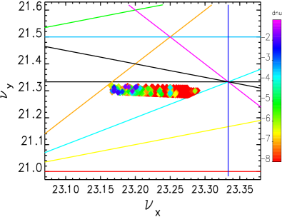
Figure 8: Betatron tune footprint with the color indicating the tune diffusion $d$.

Figure 8 shows the tune footprint corresponding to the same tracking as the frequency map in Fig. 7. As with the frequency map, the color of the tune footprint reflects the tune change in terms of the diffusion index. The lines indicate betatron resonances up to the 3rd order; higher-order resonances are not shown in this plot. Since the tunes in Fig. 8 are calculated for particles with initial coordinates in the $(x-\Delta p/p)$ phase space, the vertical tune variation arises only from the chromatic tune dependence, which is around 0.03 within $\Delta p/p$ of $\pm 4\times 10^{-3}$ as shown in Fig. 6. The horizontal tune variation is about 0.14, which is significantly greater than the chromatic tune change of 0.02 corresponding to $\Delta p/p$ of $\pm 4\times 10^{-3}$ in Fig. 6. This indicates that, after the linear chromaticity compensation, the horizontal betatron motion produces a substantial tune change, which can drive particles close to or into a resonance mode and cause particle loss. The tune change due to the particle’s transverse motion is discussed in detail in Section IV.3. Overall, the tune footprint immediately reveals the distribution of the particle tunes, which allows one to understand the tune trend due to the particle motion and subsequently adjust the design tunes to avoid approaching or crossing strong resonances.

An important feature of our symmetry concept is compensation of the chromatic beam smear at the IP. It is attained together with the linear chromaticity correction when two CCBs are placed symmetrically around the IP. One way to demonstrate this is by using the chromatic amplitude functions $W_{x,y}$, which are directly related to the chromatic derivatives of the $\beta$-functions $\partial\beta_{x,y}/\partial\delta$ wfunc_madx . Figure 9 shows the $W_{x,y}$ functions plotted over the whole ion collider ring length before and after the linear chromaticity correction, respectively. The fact that $W_{x,y}$ are close to zero at the IP indicates that the chromatic beam smear is compensated.

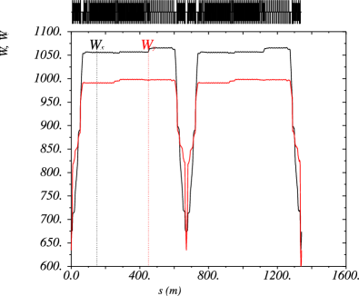
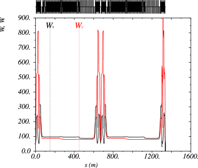
Figure 9: Horizontal and vertical chromatic amplitude functions $W_{x,y}$ plotted over the whole ion collider ring length before (top) and after (bottom) the linear chromaticity compensation.

IV.2 Comparison to the conventional distributed-sextupole scheme

To demonstrate the advantages of the proposed symmetry concept, we compared its performance with that of a more conventional “distributed-sextupole” (DS) chromaticity compensation scheme based on introducing two sextupole families in the arc FODO cells. To make a fair comparison to the CCB scheme, the CCBs were taken out of the ring optics to eliminate their chromatic contribution, and the BESs were connected directly to the FFBs. Additional FODO cells and two more sextupole families were introduced in the regions between the arcs and BESs for higher-order chromaticity correction. The phase advances between the sextupoles and between the sextupoles and IP were adjusted to cancel the sextupole nonlinear kicks and to optimize the 2nd-order chromaticity compensation as discussed in nosochkov92 . These modifications to the linear optics resulted, in particular, in higher betatron tunes but the initial horizontal $\xi_{x}$ and $\xi_{y}$ vertical natural chromaticities of -199 and -262, respectively, were still smaller than in the CCB scheme.

First, for the linear chromaticity compensation, two sextupole families were introduced in the arcs. Following the same guidelines as in the CCB case, the sextupoles were placed at locations with nearly maximum dispersion and a large difference between the horizontal and vertical $\beta$-functions. With 52 FODO cells in the two arcs of the ion collider ring, one might expect that such a globally distributed sextupole scheme can effectively reduce the sextupole strengths with a consequent suppression of the nonlinear effects introduced by the sextupole fields. However, the $\beta$-functions of a regular arc FODO cell are much smaller than those in the CCBs. Hence, even though the DS scheme has a total of 104 sextupoles compared to only 16 sextupoles in the CCB scheme, the sextupole strengths in the DS scheme are still much stronger than those in the CCB scheme. Table 2 summarizes the parameters of the two different linear chromaticity correction schemes including the values of the optical functions at the sextupole locations and the sextupole strengths.

Table 2: Comparison of the optical functions at the sextupole locations and of the sextupole strengths $\partial^{2}B_{y}/\partial x^{2}$ for 60 GeV/$c$ protons in cases of the DS and CCB-based linear chromaticity correction schemes.

Parameter	DS scheme		CCB scheme
	Sextupole family
	1	2	1	2
# of sextupoles	52	52	8	8
$\beta_{x}$ (m)	13.8	6.0	1614	2.3
$\beta_{y}$ (m)	6.0	13.8	944	1396
$D_{x}$ (m)	1.19	0.8	0.9	1.3
$\partial^{2}B_{y}/\partial x^{2}$ (T/m2)	4000	-7000	238	-288

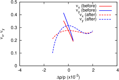
Figure 10: Chromatic dependence of the fractional betatron tunes before and after the linear chromaticity compensation using the DS approach.

Figure 10 compares the chromatic dependence of the fractional betatron tunes before and after the linear chromaticity compensation using the two sextupole families in the arc FODO cells. The slopes of the horizontal $\nu_{x}$ and vertical $\nu_{y}$ chromatic betatron tune curves are zero at $\Delta p/p=0$ after the correction, which reduces the tune variation and somewhat extends the momentum acceptance. However, the second derivatives of the corrected chromatic curves (the 2nd-order chromaticities) start dominating the tune spread and still limit the momentum acceptance. Therefore, we introduce two additional families to a total of 128 sextupoles close to the IR to compensate the 2nd-order chromaticities. For the optimal compensation, we set the phase advance between the sextupoles and IP following the approach described in nosochkov92 . The strengths of the new sextupole families were comparable to those of the two original families in Table 2.

Figure 11: Chromatic dependence of the fractional betatron tunes before and after the chromaticity compensation up to 2nd order.

Figure 11 shows the chromatic tune dependence after combining the linear and 2nd-order chromaticity compensations. Figure 11 indicates that the momentum acceptance is extended further in comparison to Fig. 10. However, the strong sextupole fields give rise to even higher-order chromaticities still leading to an impractically large tune spread. The frequency map and tune footprint for this 2nd-order DS chromaticity compensation scheme are also calculated using particle tracking and plotted in Figs. 12 and 13, respectively. Because of such a large chromatic tune spread, the particles experience numerous resonances, which limit the momentum acceptance.

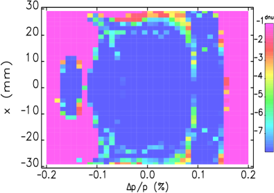
Figure 12: Frequency map in the $(x-\Delta p/p)$ phase space for the 2nd-order DS scheme with the color indicating the tune diffusion $d$.

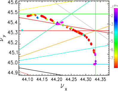
Figure 13: Tune footprint for the 2nd-order DS scheme with the color indicating the tune diffusion $d$.

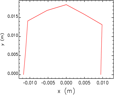
Figure 14: Dynamic aperture in the $(y-x)$ space at the entrance into one of the CCBs for the on-momentum particle.

IV.3 Dynamic aperture with the CCB scheme

A ring’s property that is equally important to its momentum acceptance is its dynamic aperture (DA), i.e. a region in the transverse plane of stable particle motion. Therefore, we study the ion collider ring’s DA for the case of the CCB-based chromaticity compensation scheme. The DA is explored by tracking particles for 1000 turns while progressively increasing their initial horizontal $(x)$ and vertical $(y)$ amplitudes until the boundary between survival and loss is found. Figure 14 shows the on-momentum particle’s DA at the entrance into one of the CCBs. The DA reaches $\sim 10$ mm horizontally and $\sim 18$ mm vertically, which is quite reasonable given the large natural chromaticities and the fact that there was no nonlinear optimization after the linear chromaticity correction. However, due to the large beam extension required to achieve the ambitiously small $\beta_{x,y}^{*}$ values at the MEIC (see Table 1), these horizontal and vertical DA sizes correspond to only $\sim 4\sigma_{x}$ and $\sim 15\sigma_{y}$, respectively. Thus, optimization of the DA using multiple sextupole and octupole families is required.

For the on-momentum particle, there is clearly no tune variation due to the chromatic tune dependence. The tune change comes from the nonlinearity of the transverse betatron motion caused by the nonlinear fields, in particular, of the sextupoles. Thus, we explore the dependence of the betatron tunes on the transverse motion. For a particle with initial transverse amplitudes $x$ and $y$, its horizontal $\nu_{x}$ and vertical $\nu_{y}$ tunes are calculated by tracking it for a number of turns. The obtained tune dependence is shown in Fig. 15: $\nu_{x}$ is plotted as a function of $x$ and $y$ at the top while $\nu_{y}$ is plotted as a function of $x$ and $y$ at the bottom.

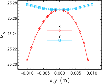
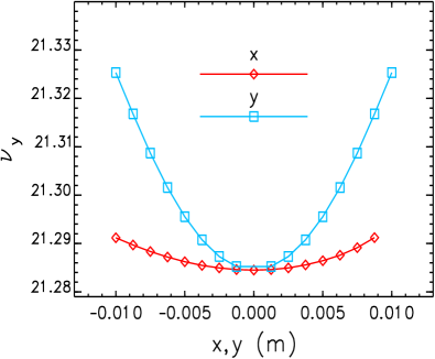
Figure 15: Dependence of the horizontal $\nu_{x}$ (top) and vertical $\nu_{y}$ (bottom) betatron tunes on the initial transverse amplitudes $x$ and $y$.

The simulations show that, after the sextupole compensation, there is a large amplitude-dependent tune shift. This is due to the fact the nonlinearity of the sextupole fields causes stronger focusing of the particles with larger transverse amplitudes. As seen from Fig. 15, $\nu_{x}$ and $\nu_{y}$ change from the design values by 0.08 (the red line in the top plot) and 0.04 (the blue line in the bottom plot), respectively, within $x$ and $y$ of about $\pm 10$ mm. Such a large tune deviation can easily drive particles to approach or cross betatron resonances, which inevitably causes their loss. The tune shift with amplitude limits the ring’s DA, especially in the horizontal direction due to the large horizontal beam extension in the ion collider ring (the maximum horizontal rms beam size $\sigma_{x}$ along the ring is 3.2 mm). Figure 15 also shows that there is very little coupling between the two transverse dimensions: $\nu_{x}$ is almost independent of the vertical motion (the blue line in the top plot of Fig. 15) while $\nu_{y}$ is unaffected by the horizontal motion (the red line in the bottom plot of Fig. 15).

A straightforward mechanism to compensate the amplitude-dependent tune shift caused by the sextupoles is to introduce octupoles. Depending on the octupole locations, both the amplitude dependent tune shift and higher-order chromaticities can be controlled by adjusting the octupole strengths. Since the momentum acceptance is large enough after the linear chromaticity correction with the CCBs, we focus on compensation of the amplitude-dependent tune shift. Therefore, octupole families should be placed in dispersion-free regions to leave the chromatic correction unaffected. Also, to reduce the required octupole strengths, they should be placed at large $\beta$-function points. Following these considerations, three families of octupoles are introduced in the BES and FFB regions. It was the most convenient for us to find a solution for the octupole strengths that provide compensation of the 1st-order amplitude dependent tune shifts, using the arbitrary-order expansion tools of COSY Infinity berz_cosy . After this compensation, the horizontal and vertical tune variations are again obtained as functions of the initial transverse amplitudes $x$ and $y$ from particle tracking and are plotted in Fig. 16. Compared to the tune changes of 0.08 and 0.04 within the transverse amplitude of about $\pm 10$ mm in Fig. 15, the horizontal and vertical tune changes are now 0.04 and 0.03, respectively, within an amplitude range of over $\pm 15$ mm. Consequently, the DA is increased as shown by the blue line in Fig. 17 in comparison to the red line without the octupole optimization.

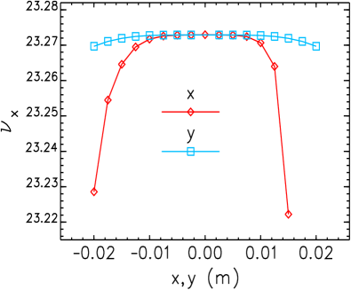
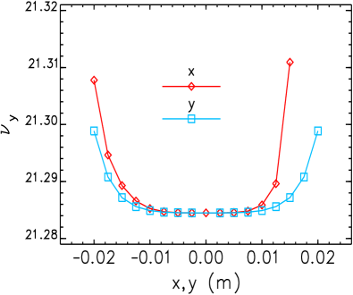
Figure 16: $\nu_{x}$ (top) and $\nu_{y}$ (bottom) as functions of $x$ and $y$ after compensation of the 1st-order amplitude dependent tune shifts.

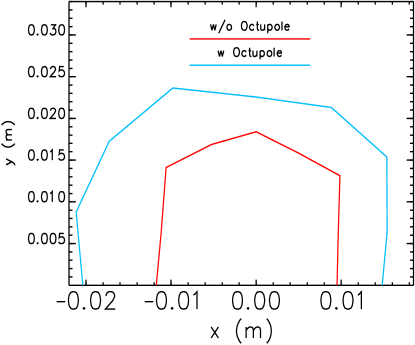
Figure 17: Dynamic aperture in the $(y-x)$ space at the entrance into one of the CCBs for the on-momentum particle without (red) and with (blue) the octupole compensation of the 1st-order amplitude-dependent tune shift.

After the octupole compensation, the limitation on the DA comes from the effect of the 2nd-order amplitude-dependent tune shift, which starts dominating the tune behavior in Fig. 16. This provides a guideline that the DA can be further enhanced by considering and optimizing the 1st-, 2nd-, and even higher-order amplitude-dependent effects. One possibility for future studies is to use a genetic algorithm to optimize the DA directly by simultaneously adjusting multiple sextupole and octupole families borland10 . Note that magnet errors are not included in the above simulations. Addressing the question of error tolerances is the subject of our future studies.

V Conclusions

We proposed a new symmetry-based interaction region concept for a high-luminosity collider ring design. Such a symmetric design allows simultaneous compensation of (a) the betatron tune spreads due to the 1st-order chromaticities, (b) chromatic beam smear at the IP, i.e. chromatic spread of focal point, and (c) other 2nd-order aberrations to the particle trajectory at the IP and on average over one turn, such as the 2nd-order dispersion effect and sextupole-generated beam smear due to the beam size. According to this concept, two specially-designed symmetric Chromaticity Compensation Blocks (CCBs) are placed symmetrically around an IP. Each CCB induces an angle spread in the passing beam such that it cancels the chromatic kick of the final focusing quadrupoles. We developed an analytic description of this approach and explicitly formulated 2nd-order aberration compensation conditions at the IP. We verified our concept by developing a specific interaction region design and applying our chromaticity compensation scheme to a challenging case of a high-chromaticity small-$\beta^{*}$ MEIC ion collider ring des_rep12 . We then compared performance of our symmetric CCB approach with that of the conventional distributed-sextupole chromaticity compensation scheme. The CCB approach resulted in a much greater momentum acceptance with a smaller number of weaker sextupoles. The dynamic aperture after the chromaticity correction is reasonably large, especially given the large natural chromaticities. We identified the factors limiting the dynamic aperture, namely, the 1st- and higher-order amplitude-dependent tune shifts, and demonstrated an approach to dynamic aperture optimization using octupole families. Further optimization may be needed depending on the specific requirements. Evaluation of the error impact will be addressed in the future studies.

VI Acknowledgments

This work was supported in part by the U.S. Department of Energy Small Business Technology Transfer Grant DE-SC0006272. This manuscript has been authored by Jefferson Science Associates, LLC under Contract No. DE-AC05-06OR23177 with the U.S. Department of Energy. The United States Government retains and the publisher, by accepting the article for publication, acknowledges that the United States Government retains a non-exclusive, paid-up, irrevocable, world-wide license to publish or reproduce the published form of this manuscript, or allow others to do so, for United States Government purposes. We are grateful to C.M. Ankenbrandt, S.A. Bogacz, A.M. Hutton, G.A. Krafft, F.C. Pilat, and T.J. Satogata for their help and advice.

References

- (1) Science Requirements and Conceptual Design for a Polarized Medium Energy Electron-Ion Collider at Jefferson Lab, edited by Y. Zhang and J. Bisognano (2012) [http://casa.jlab.org/meic/files/MEIC_Report.pdf].
- (2) eRHIC Zeroth-Order Design Report, edited by M. Farkhondeh and V. Ptitsyn (2004) [http:// web.mit.edu/eicc/DOCUMENTS/eRHIC_ZDR.pdf].
- (3) Handbook of Accelerator Physics and Engineering, edited by A.W. Chao and M. Tigner (World Scientific, Singapore, 2006).
- (4) Y. Nosochkov, F. Pilat, and T. Sen, in Proceedings of Workshop on Stability of Particle Motion in Storage Rings, Upton, NY, 1992, AIP Conf. Proc. No. 292 (AIP, Melville, NY, 1992), p. 135.
- (5) KEKB B-Factory Design Report, KEK Report No. 95-7 (1995).
- (6) P. Raimondi and A. Seryi, Phys. Rev. Lett. 86, 3779 (2001).
- (7) Y.I. Alexahin, E. Gianfelice-Wendt, V.V. Kashikhin, N.V. Mokhov, A.V. Zlobin, and V.Y. Alexakhin, Phys. Rev. ST Accel. Beams 14, 061001 (2011).
- (8) S.Y. Lee, Accelerator Physics (World Scientific, Singapore, 1999).
- (9) Ya.S. Derbenev, presentation at the 2007 Low-Emittance Muon Collider Workshop (LEMC’07), Batavia, IL [http://www.muonsinc.com/mcwfeb07/presentations /Derbenev_021307.doc].
- (10) G. Wang, Ya.S. Derbenev, S.A. Bogacz, P. Chevtsov, A. Afanasev, C.M. Ankenbrandt, V. Ivanov, and R.P. Johnson, in Proceedings of the 2009 Particle Accelerator Conference, Vancouver, Canada (IEEE, Piscataway, NJ, 2009), WE6PFP064, p. 2649.
- (11) V.S. Morozov and Ya.S. Derbenev, in Proceedings of the 2011 International Particle Accelerator Conference, San Sebastian, Spain (EPS-AG, San Sebastian, Spain, 2011), THPZ017, p. 3723.
- (12) F. Lin, Ya.S. Derbenev, V.S. Morozov, and Y. Zhang, in Proceedings of the 2012 International Particle Accelerator Conference (IPAC’12), New Orleans, LA (IEEE, New York, NY, 2012), TUPPC099, p. 1389.
- (13) E.D. Courant and H.S. Snyder, Ann. Phys. 3, 1 (1958).
- (14) V.S. Morozov, R. Ent, P. Nadel-Turonski and C.E. Hyde, in Proceedings of the 2012 International Particle Accelerator Conference, New Orleans, Louisiana, USA, 2012 (Ref. lin_ipac12 ), TUPPR080, p. 2011.
- (15) J. Laskar, in Proceedings of 3DHAM95, NATO Advanced Study Institutes (Kluwer Academic Publishers, Dordrecht, The Netherlands, 1999), p. 134.
- (16) M. Borland, ANL/APS Report No. LS-287 (2000) [http://www.aps.anl.gov/Science/Publications/lsnotes/ ls287.pdf].
- (17) C. Steier and W. Wan, in Proceedings of the 2010 International Particle Accelerator Conference, Kyoto, Japan (ICR, Kyoto, 2010), THPE095, p. 4746.
- (18) H. Grote and F.C. Iselin, CERN Report No. CERN/SL/ 90-13 (AP) (Rev. 5) (1996).
- (19) K. Makino and M. Berz, Nucl. Instrum. Methods Phys. Res., Sect. A 558, 346 (2006).
- (20) M. Borland, V. Sajaev, L. Emery, and A. Xiao, ANL/APS Report No. LS-319 (2010) [http:// www.ipd.anl.gov/anlpubs/2010/08/67580.pdf].