Suppression of superconductivity by Neel-type magnetic fluctuations in the iron pnictides

Abstract

Motivated by recent experimental detection of Neel-type ($(\pi,\pi)$) magnetic fluctuations in some iron pnictides, we study the impact of competing $\left(\pi,\pi\right)$ and $\left(\pi,0\right)$ spin fluctuations on the superconductivity of these materials. We show that, counter-intuitively, even short-range, weak Neel fluctuations strongly suppress the $s^{+-}$ state, with the main effect arising from a repulsive contribution to the $s^{+-}$ pairing interaction, complemented by low frequency inelastic scattering. Further increasing the strength of the Neel fluctuations leads to a low-$T_{c}$ d-wave state, with a possible intermediate $s+id$ phase. The results suggest that the absence of superconductivity in a series of hole-doped pnictides is due to the combination of short-range Neel fluctuations and pair-breaking impurity scattering, and also that $T_{c}$ of optimally doped pnictides could be further increased if residual $\left(\pi,\pi\right)$ fluctuations were reduced.

The proximity of the superconducting state (SC) to a “stripe” spin-density wave instability (SDW) in the phase diagrams of the recently discovered iron-based superconductors reviews (FeSC) prompted the proposal that SDW spin fluctuations provide the pairing mechanism magnetic . Indeed, the Fermi surface (FS) of many iron pnictides consists of electron pockets displaced from central hole pockets by the SDW ordering vector $\mathbf{Q}_{\mathrm{SDW}}=\left(\pi,0\right)/\left(0,\pi\right)$ (see Fig. 1). In this situation, even weak SDW fluctuations may overcome a strong on-site repulsion giving rise to an $s^{+-}$ SC state, in which the gap function has one sign on the electron pockets and another sign on the hole pockets reviews_pairing .

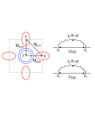
Figure 1: (left panel) Schematic Fermi surface configuration in the 1-Fe Brillouin zone, with two central hole pockets and two electron pockets. (right panel) Self-energy diagrams of the Eliashberg equations: normal component (upper panel) and anomalous component (lower panel).

However, the two electron pockets in Fig. 1 are connected by the momentum $\mathbf{Q}_{\mathrm{Neel}}=\left(\pi,\pi\right)$ suggesting that Neel-type magnetic fluctuations may also be important Kuroki09 . These fluctuations favor a d-wave SC state in which the gap function has opposite sign in the two electron pockets. On the theory side, first-principle and Hartree-Fock calculations find that the Neel state is locally stable, but with a higher energy than the SDW state Johannes09 ; Bascones11 , while random phase approximation (RPA) calculations performed in the paramagnetic phase find a peak in the magnetic susceptibility at $\mathbf{Q}_{\mathrm{Neel}}$, which is however weaker than the peak at $\mathbf{Q}_{\mathrm{SDW}}$ Graser10 .

Experimentally, neutron scattering measurements Mn_neutron revealed that even at small $x$, $\mathrm{Ba}\left(\mathrm{Fe_{1-x}Mn_{x}}\right)_{2}\mathrm{As_{2}}$ exhibits spin fluctuations peaked at $\mathbf{Q}_{\mathrm{Neel}}$, in addition to the SDW fluctuations peaked at $\mathbf{Q}_{\mathrm{SDW}}$. NMR measurements Mn_NMR confirmed that these Neel fluctuations couple to the conduction electrons. Because the entire family of “in-plane” hole-doped $\mathrm{Ba}\left(\mathrm{Fe_{1-x}}M_{\mathrm{x}}\right)_{2}\mathrm{As_{2}}$ compounds ($M=\mathrm{Mn}$, Cr, Mo) hole_doped_series displays SDW order at $x=0$ and Neel order at $x=1$, we expect that competing Neel and SDW fluctuations will be found across the whole material family. Intriguingly, superconductivity has not been reported in these materials to date Mn_pressure , in contrast to the electron-doped counterparts $M=\mathrm{Co}$, Ni, Rh, Pt, Cu, where SC is always observed Canfield_transition_metals .

There is also indirect evidence for Neel fluctuations in the extremely electron-doped $A_{y}\mathrm{Fe_{2-x}Se_{2}}$ compounds KFe2Se2 . In these materials, the near absence of FS pockets in the center of the Brillouin zone suggests that SDW fluctuations and the $s^{+-}$ state are disfavored, while the square-like shape of the electron pockets is expected to enhance the $\left(\pi,\pi\right)$ fluctuations Scalapino12 . Chemical substitution on the $A$ site or application of pressure Balatsky12 , can create a small pocket in the center of the Brillouin zone, which could support $\left(\pi,0\right)$ fluctuations and $s^{+-}$ SC.

The effect of competing spin fluctuations on FeSCs is thus of experimental and theoretical interest. In this paper, we address the problem via a multi-band Eliashberg approach Eliashberg ; Carbotte in which the effect of spin fluctuations on electrons is determined from the one-loop self energy (see Fig. 1). This approximation has been extensively employed in studies of cuprates Monthoux92 ; Millis92 ; critical_pairing , ferromagnetic SC Roussev01 , and pnictides eliashberg_pnictides . Our calculation goes beyond previous work eliashberg_pnictides by incorporating both SDW and Neel fluctuations, including the Coulomb pseudo-potential, and using the experimentally determined spin fluctuation spectrum instead of the single-pole approximation employed previously.

We find that the Coulomb pseudo-potential has only a weak effect on the dominant $s^{+-}$ state but that even weak, short-range Neel fluctuations strongly suppress the transition temperature $T_{c}^{\mathrm{s-wave}}$. If sufficiently strong, the Neel fluctuations may induce a d-wave state, but the transition temperature is found to be much lower than the optimal $T_{c}$ for the $s^{+-}$ state. The transition between $s^{+-}$ and $d$-SC may either occur via an intermediate time reversal symmetry-breaking $s+id$ state Stanev10 ; s_plus_id or, if the impurity scattering is stronger, via an intermediate non-SC state separating the two regions (see Fig. 2).

To gain insight into the results, we use the functional derivative methods of Bergmann and Rainer Bergmann_Rainer ; Millis88 . We find that the strong suppression of the $s^{+-}$ state comes mostly from a repulsive $s^{+-}$ pairing interaction induced by the Neel fluctuations, although pair-breaking inelastic scattering plays some role. Finally, we discuss the implications of our results not only to the SC of the in-plane hole-doped pnictides, but also to the value of $T_{c}$ in the FeSCs in general.

Our model consists of a two-dimensional FS with two central hole pockets ($\Gamma$, density of states $N_{\Gamma}$) and two electron pockets ($X$ and $Y$, density of states $N_{X}$) displaced from the center by the momenta $\left(\pi,0\right)$ and $\left(0,\pi\right)$ (Fig. 1) Maiti11 . For simplicity, hereafter we assume that these two hole pockets are degenerate - our results do not depend on this simplification. Following Ref. Vekhter11 , we set $r=N_{X}/N_{\Gamma}=0.65$. The electrons are coupled to two types of low-energy bosonic excitations, namely, SDW spin fluctuations peaked at $\left(\pi,0\right)/\left(0,\pi\right)$ and Neel spin fluctuations peaked at $\left(\pi,\pi\right)$. Experiment (Refs.Mn_neutron ; INS_pnictides ) indicates that in the paramagnetic phase these excitations are described by diffusive dynamic susceptibilities:

$$\chi_{i}^{-1}\left(\mathbf{Q}_{i}+\mathbf{q},\Omega_{n}\right)=\xi_{i}^{-2}+q^{2}+\gamma_{i}^{-1}\left|\Omega_{n}\right|$$ (1)

Here, $\mathbf{q}$ is the momentum deviation from the ordering vector $\mathbf{Q}_{i}$ (all lengths are in units of the lattice parameter $a$) and $\Omega_{n}$ is the bosonic Matsubara frequency. The quantity that actually enters the Eliashberg equations is the spectral function integrated over the momentum component $q_{\parallel}$ parallel to the FS and evaluated at $q_{\bot}=0$, i.e. $A_{\mathrm{Neel}}\left(\omega\right)=\int dq_{\parallel}\mathrm{Im}\chi_{\mathrm{Neel}}\left(q_{\parallel},\omega\right)$. This spectral function gives rise to the Matsubara-axis interaction $a^{(i)}\left(\Omega_{n}\right)=\xi_{i}/\sqrt{1+\left|\Omega_{n}\right|\gamma_{i}^{-1}\xi_{i}^{2}}$ which enters the Eliashberg equations as described below. Note that the orbital character of the low energy states varies with position around the FS. In the Eliashberg formalism the resulting angular dependence of the interaction parameters is averaged over the FS, so as shown in the Supplementary Material the variation in the orbital character only affects the values of the effective coupling constants.

The spin fluctuations in each momentum channel $i$ are described by two parameters: the Landau damping $\gamma_{i}$, which sets the energy scale, and the correlation length $\xi_{i}$, which sets both the strength and the spatial/temporal correlations of the spin fluctuations. We will tune the spectrum by varying $\xi_{i}$. Because the Landau damping originates from the low-energy decay of the spin excitations into electron-hole pairs, $\gamma_{i}$ is determined by the electron-boson coupling constant $g_{i}$ and the densities of states. The coupling $g_{\mathrm{SDW}}$ is set to yield $T_{c,0}^{\mathrm{s-wave}}\approx 30$ K. Following the experimental results of Ref. Mn_neutron , we use $\gamma_{\mathrm{Neel}}/\gamma_{\mathrm{SDW}}\approx 0.33$ with $\gamma_{\mathrm{SDW}}\approx 25$ meV; the value of $g_{\mathrm{Neel}}$ follows from the relationship between $\gamma_{\mathrm{Neel}}/\gamma_{\mathrm{SDW}}$ and $g_{\mathrm{Neel}}/g_{\mathrm{SDW}}$. Finally, we set $\xi_{\mathbf{\mathrm{SDW}}}=5a$ throughout our calculations, varying the correlation length of the Neel fluctuations $\xi_{\mathrm{Neel}}$. Our results do not change significantly for smaller values of $\xi_{\mathrm{SDW}}$.

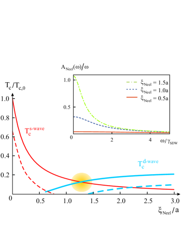
Figure 2: Transition temperatures $T_{c}$ of the s-wave (red/light curve) and d-wave (blue/heavy curve) states as function of the Neel magnetic correlation length $\xi_{\mathrm{Neel}}$, for $r=0.65$, $\gamma_{\mathrm{Neel}}/\gamma_{\mathrm{SDW}}=0.33$, $\lambda_{\mathrm{Neel}}/\lambda_{\mathrm{SDW}}=2$, and $\mu^{*}=0.8$. $T_{c,0}\approx 0.1\gamma_{\mathrm{SDW}}$ is the $s^{+-}$ transition temperature for $\xi_{\mathrm{Neel}}=0$. The shaded area denotes the regime where the two states have similar transition temperatures and a possible $s+id$ state may occur. The dashed lines show the behavior of the system in the presence of impurity scattering, with $\tau^{-1}\approx 0.1T_{c,0}$. The inset shows the frequency dependence of the spectral function $A_{\mathrm{Neel}}\left(\omega\right)$ of the Neel fluctuations for different values of $\xi_{\mathrm{Neel}}$.

To obtain the transition temperatures in the $s$ and $d$-wave channels we linearize the Eliashberg equations in the superconducting quantities and solve the resulting equations for the anomalous component $W_{\alpha,n}$ and the normal component $Z_{\alpha,n}=\mathrm{Im}\Sigma_{\alpha,n}^{N}/i\omega_{n}$ of the self-energy (the real part of $\Sigma^{N}$ just renormalizes the band dispersions, possibly differently for different pockets Eliashberg ; Carbotte ; Benfatto11 ). These quantities are averaged over each Fermi pocket becoming functions only of the Fermi pocket label $\alpha$ and the fermionic Matsubara frequency $\omega_{n}=\left(2n+1\right)\pi T$. With the aid of the auxiliary “gap functions” $\bar{\Delta}_{\Gamma,n}\equiv\frac{W_{\Gamma,n}}{Z_{\Gamma,n}\left|\omega_{n}\right|\sqrt{N_{X}}}$ and $\bar{\Delta}_{(X/Y),n}\equiv\frac{W_{(X/Y),n}}{Z_{X,n}\left|\omega_{n}\right|\sqrt{N_{\Gamma}}}$, the linearized gap equation is expressed as a matrix equation in Matsubara (indices $n,m$) and band (indices $\alpha,\beta$) spaces $\sum_{m,\beta}K_{nm}^{\alpha\beta}\bar{\Delta}_{\beta,m}=0$, with the kernel:

$$\left(K_{nm}^{\alpha\beta}\right) = -\left(\begin{array}[]{ccc}\delta_{nm}\frac{Z_{\Gamma,n}\left|\omega_{n}\right|}{T}&\frac{\lambda_{\mathrm{SDW}}}{2}a_{nm}^{(1)}&\frac{\lambda_{\mathrm{SDW}}}{2}a_{nm}^{(1)}\\ \lambda_{\mathrm{SDW}}a_{nm}^{(1)}&\delta_{nm}\frac{Z_{X,n}\left|\omega_{n}\right|}{T}&\lambda_{\mathrm{Neel}}a_{nm}^{(2)}\\ \lambda_{\mathrm{SDW}}a_{nm}^{(1)}&\lambda_{\mathrm{Neel}}a_{nm}^{(2)}&\delta_{nm}\frac{Z_{X,n}\left|\omega_{n}\right|}{T}\end{array}\right)$$ (9)

$$-\frac{1}{2}\left[\frac{\mu^{*}}{1+r}-\frac{\tau^{-1}}{T}\frac{\delta_{nm}}{r}\right]\left(\begin{array}[]{ccc}2&\sqrt{r}&\sqrt{r}\\ 2\sqrt{r}&r&r\\ 2\sqrt{r}&r&r\end{array}\right)$$

Here we have introduced the matrix elements coming from the bosonic modes $a_{nm}^{(i)}=a^{i}(\omega_{n}-\omega_{m})$ ($i=1$ corresponds to SDW and $i=2$, to Neel fluctuations) and the dimensionless coupling constants $\lambda_{\mathrm{SDW}}=2g_{\mathrm{SDW}}^{2}\sqrt{N_{\Gamma}N_{X}}$, $\lambda_{\mathrm{Neel}}=g_{\mathrm{Neel}}^{2}N_{X}$. $T$ is the temperature. We also introduce an upper frequency cutoff $\Lambda=8\gamma_{\mathrm{SDW}}$, corresponding to the energy scale of the bottom/top of the electron/hole bands, and we assume that $\mu^{*}$ is a bare Coulomb interaction renormalized in the standard way by higher energy processes. $\tau^{-1}$ is the scattering rate associated with non-magnetic point impurities and the $Z_{\alpha,n}$ functions are obtained analytically (see Supplementary Material). The Coulomb pseudo-potential favors solutions with $\sum_{\alpha}N_{\alpha}\Delta_{\alpha}=0$.

Reflecting the tetragonal symmetry of the system, the matrix equation supports two different types of solution: the s-wave state $\bar{\Delta}_{X,n}=\bar{\Delta}_{Y,n}$, with either $s^{++}$ ($\bar{\Delta}_{\Gamma,n}\propto\bar{\Delta}_{X,n}$) or $s^{+-}$ ($\bar{\Delta}_{\Gamma,n}\propto-\bar{\Delta}_{X,n}$) structure, and the d-wave state $\bar{\Delta}_{X,n}=-\bar{\Delta}_{Y,n}$. The solution in a given symmetry channel is obtained when the largest eigenvalue $\eta$ of the matrix (9) vanishes. Since our calculations never yield an $s^{++}$ state, we use the terms s-wave and $s^{+-}$ to refer to the same state. Due to limitations of the size of the matrices that can be diagonalized, and since the matrix size scales as $\Lambda/T$, we resolve $T_{c}\gtrsim 10^{-3}\gamma_{\mathrm{SDW}}$. Hereafter, we set $\lambda_{\mathrm{SDW}}=0.4$ and the Coulomb pseudo-potential $\mu^{*}=0.8$, which gives, in the absence of competing Neel fluctuations, $T_{c,0}^{\mathrm{s-wave}}\approx 30$K and implies $\lambda_{\mathrm{Neel}}=0.8$.

Fig. 2 shows our principal results: the dependence of the SC transition temperature $T_{c}$ on the strength of Neel fluctuations (parametrized by the Neel correlation length $\xi_{\mathrm{Neel}}$). The light solid line (red online) shows the transition temperature $T_{c}^{\mathrm{s-wave}}$ for the $s^{+-}$ channel in the absence of impurity scattering. Surprisingly, even weak, short-range fluctuations strongly suppress $s^{+-}$ SC, but once $T_{c}^{\mathrm{s-wave}}$ has been substantially reduced, the additional suppression effect caused by further increasing $\xi_{\mathrm{Neel}}$ is small. Sufficiently strong Neel correlations produce a d-wave solution (heavier solid line, blue online) with $T_{c}^{\mathrm{d-wave}}$ that eventually becomes larger than $T_{c}^{\mathrm{s-wave}}$ but always remains small compared to the maximum $T_{c}^{\mathrm{s-wave}}$. In our linearized theory the transition between s-wave and d-wave superconductors appears as a discontinuous change in the nature of the state, but the considerations of Stanev10 suggest that nonlinear terms not included here will generate an intermediate $s+id$ state (shaded area). The dashed lines show the behavior in the presence of impurity scattering, which is pair-breaking for both $s^{+-}$ and $d$-wave superconductivity. Sufficiently strong impurity scattering can disconnect the two SC states, leaving an intermediate non-SC regime.

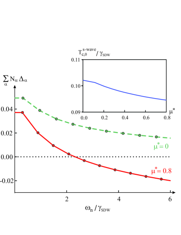
Figure 3: Averaged $s^{+-}$ gap function $\sum_{\alpha}N_{\alpha}\Delta_{\alpha}$ across the different pockets at $T_{c,0}^{\mathrm{s-wave}}$ as function of Matsubara frequency $\omega_{n}$ (in units of $\gamma_{\mathrm{SDW}}$), for $\mu^{*}=0$ (green/dashed curve) and $\mu^{*}=0.8$ (red/solid curve). The inset shows $T_{c,0}^{\mathrm{s-wave}}$ (in units of $\gamma_{\mathrm{SDW}}$) as function of $\mu^{*}$. Although here we used $\xi_{\mathrm{Neel}}=0$, a similar behavior holds for $\xi_{\mathrm{Neel}}\neq 0$.

We also analyze the impact of the Coulomb pseudo-potential $\mu^{*}$ on the $s^{+-}$ state - the d-wave state avoids the Coulomb repulsion. Fig. 3 shows the pocket-averaged $s^{+-}$ gap function $\sum_{\alpha}N_{\alpha}\Delta_{\alpha}$ both in the presence and in the absence of $\mu^{*}$. To avoid the local repulsion, the averaged order parameter changes sign at a non-zero Matsubara frequency, although the sign of each individual gap does not necessarily change. This is the multi-band analogue of the response of a single-band s-wave superconductor to the local repulsion. For all values of $\xi_{\mathrm{Neel}}$ we have studied, neither $\Delta_{n=0}$ nor $T_{c}^{\mathrm{s-wave}}$ (shown in the inset) are substantially altered by $\mu^{*}$, in agreement with the weak-coupling analysis of Ref. Mazin_Schmalian .

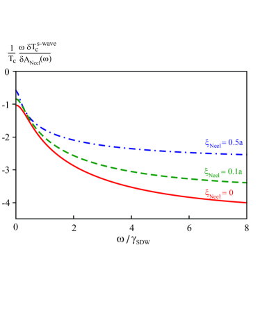
Figure 4: Functional derivative $T_{c}^{-1}\omega\delta T_{c}^{\mathrm{s-wave}}/\delta A_{\mathrm{Neel}}\left(\omega\right)$ as function of frequency $\omega$ (in units of $\gamma_{\mathrm{SDW}}$) for the cases $\xi_{\mathrm{Neel}}=0$ (red/solid line), $\xi_{\mathrm{Neel}}=0.1a$ (green/dashed line), and $\xi_{\mathrm{Neel}}=0.5a$ (blue/dotted dashed line).

We now turn to the physics of the decrease of $T_{c}^{\mathrm{s-wave}}$ caused by Neel fluctuations. Increasing $\xi_{\mathrm{Neel}}$ increases the spin fluctuation intensity and changes its functional form (see the inset of Fig. 2). To analyze how different frequency regions of the Neel spectral function  affect $T_{c}^{\mathrm{s-wave}}$, we follow Ref. Bergmann_Rainer ; Millis88 and calculate the functional derivative

$$\frac{1}{T_{c}}\frac{\omega\,\delta T_{c}}{\delta A_{\mathrm{Neel}}\left(\omega\right)}=\left[\hat{\Delta}\frac{\omega\,\delta\hat{K}}{T_{c}\,\delta A_{\mathrm{Neel}}\left(\omega\right)}\hat{\Delta}\right]/\left(-\frac{\partial\eta}{\partial T_{c}}\right)_{\eta=0}$$ (10)

for different values of $\xi_{\mathrm{Neel}}$, as shown in Fig. 4. Previous work Bergmann_Rainer ; Millis88 has shown that the low frequency regime captures the pair-breaking effects of inelastic scattering while the high frequency regime expresses the changes to the pairing interaction. The larger magnitude of $\delta\log T_{c}/\delta A_{\mathrm{Neel}}$ at high frequencies shows that in the pnictides the dominant effect of the Neel fluctuations is to provide a negative contribution to the $s^{+-}$ pairing interaction, with the extra pair-breaking effect of the induced low frequency inelastic scattering being less important. Because Fig. 4 shows that the logarithmic derivative of $T_{c}$ is a slow function of $\xi_{\mathrm{Neel}}$ we conclude that the initial steep drop and subsequent flattening of the $T_{c}$ curve shown in Fig. 2 is due in large part to the variation of $T_{c}$ itself. Additionally, as $\xi_{\mathrm{Neel}}$ is increased the Neel fluctuation spectrum shifts to lower frequencies (see the inset of Fig. 2), where the pair-breaking is less effective. However, additional physics is also at play. In the weak-coupling limit of two effective competing pairing interactions $\lambda_{s}$ and $\lambda_{d}$ we obtain $T_{c}\propto\exp\left[-1/\left(\sqrt{\lambda_{s}^{2}+\lambda_{d}^{2}}-\lambda_{d}\right)\right]$ so

$$\frac{d\log T_{c}}{d\lambda_{d}}\propto-\frac{1}{\left(\lambda_{s}^{2}+\lambda_{d}^{2}-\lambda_{d}\sqrt{\lambda_{s}^{2}+\lambda_{d}^{2}}\right)}$$ (11)

which is larger in magnitude for larger $\lambda_{d}$, implying an opposite ordering of the curves to that seen in Fig. 4. Our Eliashberg results and Eq. 11 differ because the gap function self-consistently adjusts to the pairing potential, so that for larger $\xi_{\mathrm{Neel}}$ the gap function decreases more rapidly with frequency, thereby minimizing the depairing effects of the Neel fluctuations (see Supplementary Material).

Our results offer a possible explanation for the puzzling behavior of the hole-doped $\mathrm{Ba}\left(\mathrm{Fe_{1-x}}M_{\mathrm{x}}\right)_{2}\mathrm{As_{2}}$ series ($M=\mathrm{Mn}$, Cr, Mo) hole_doped_series , which, in contrast to its electron-doped counterpart ($M=\mathrm{Co}$, Ni, Rh, Pt, Cu) Canfield_transition_metals , does not display SC. The short-range Neel fluctuations induced by the dopants, which were observed experimentally for low concentrations of $M=\mathrm{Mn}$ Mn_neutron ; Mn_NMR , suppress the $s^{+-}$ state without giving rise to a high-temperature d-wave state. This low-$T_{c}$ $s^{+-}$ state, in turn, can be easily suppressed, for example by impurity scattering or by another competing ordered state, such as the SDW state FernandesPRB10 ; Vorontsov09 observed at low $x$. We suggest that improving the purity of the samples and applying pressure to suppress the SDW state may reveal either a weakened $s^{+-}$ state or perhaps a low $T_{c}$ d-wave state. Similarly, in the extremely electron-doped $A_{y}\mathrm{Fe_{2-x}Se_{2}}$ systems KFe2Se2 ; ARPES_Fe2Se2 ; Keimer_Fe2Se2 , where for small $y$ the hole pocket is generally absent and d-wave superconductivity is discussed, adding holes by changing $A$ Scalapino12 or by applying pressure Balatsky12 should produce the reverse competition. Interestingly, recent pressure experiments found two separate SC domes in $\mathrm{K}_{0.8}\mathrm{Fe_{1.78}Se_{2}}$ Mao_FeSe , which could be related to the behavior shown in Fig. 2 (dashed lines). Indeed, pressure changes the shapes of the Fermi pockets, which affects the relative strength of SDW and Neel fluctuations.

More generally, since most FeSC compounds have two matching electron pockets separated by $\mathbf{Q}_{\mathrm{Neel}}$ even at optimal doping compositions, we expect at least weak Neel-type fluctuations. Indeed, recent Raman data indicate that a d-wave instability, presumably originated from these Neel fluctuations, compete with the $s^{+-}$ state of optimally-doped FeSC raman_mode . However, our findings show that these weak $\left(\pi,\pi\right)$ fluctuations strongly suppress $T_{c}^{\mathrm{s-wave}}$. This suggests that the highest $T_{c}$ in several FeSCs can be potentially enhanced if the $\left(\pi,\pi\right)$ fluctuations are minimized. One possible route is to make the sizes and shapes of the two electron pockets unequal, via, for example, a tetragonal symmetry breaking Fernandes12 . Interestingly, torque magnetometry measurements found such a tetragonal symmetry breaking above $T_{c}$ in some optimally doped FeSCs Matsuda12 . In Ref. Kuo12 , it was also observed that a small strain applied along the orthorhombic axis can enhance $T_{c}$.

In summary, our results open a new route to explore unconventional superconductivity in multi-band systems by controlling competing spin fluctuations. In particular, Neel fluctuations have a strong effect on the $s^{+-}$ state of the FeSCs, rapidly reducing $T_{c}$ and potentially driving a transition from s-wave to d-wave SC (Fig. 2). Depending on the strength of impurity scattering, more exotic states can emerge, such as the $s+id$ state Stanev10 , although this might also arise from other mechanisms s_plus_id . Notice also that the lower $T_{c}$ solution, even if not present in the ground state, will give rise to a collective excitation which can in principle be detected by Raman scattering raman_mode ; collective_mode .

We thank P. Canfield, A. Chubukov, A. Goldman, I. Eremin, A. Kreyssig, B. Lau, R. McQueeney, D. Pratt, J. Schmalian, and G. Tucker for useful discussions. RMF is supported by the NSF Partnerships for International Research and Education (PIRE) program OISE-0968226 and AJM by NSF-DMR-1006282.

Supplementary material for “Suppression of superconductivity by Neel-type magnetic fluctuations in the iron pnictides”

I Formulation and Solution of Eliashberg Equations

I.1 Formulation of Equations

The low-energy action describing the coupling between the electrons and the SDW and Neel fluctuations is conveniently expressed in terms of the Nambu operator $\Psi_{\mathbf{k}}^{\dagger}=\left(\begin{array}[]{cccccccc}c_{\Gamma,\mathbf{k}\uparrow}^{\dagger}&c_{\Gamma,-\mathbf{k}\downarrow}^{\phantom{}}&c_{\Gamma^{\prime},\mathbf{k}\uparrow}^{\dagger}&c_{\Gamma^{\prime},-\mathbf{k}\downarrow}^{\phantom{}}&c_{X,\mathbf{k}\uparrow}^{\dagger}&c_{X,-\mathbf{k}\downarrow}^{\phantom{}}&c_{Y,\mathbf{k}\uparrow}^{\dagger}&c_{Y,-\mathbf{k}\downarrow}^{\phantom{}}\end{array}\right)$, where $c_{\Gamma,\mathbf{k}\sigma}$, $c_{\Gamma^{\prime},\mathbf{k}\sigma}$, $c_{X,\mathbf{k}\sigma}$, and $c_{Y,\mathbf{k}\sigma}$ correspond to operators on the $\Gamma$ and $\Gamma^{\prime}$ hole pockets, on the $X$ electron pocket at $\left(\pi,0\right)$ , and on the $Y$ electron pocket at $\left(0,\pi\right)$, respectively. We have:

$$S=\int_{k}\Psi_{k}^{\dagger}\left(\hat{\varepsilon}_{\mathbf{k}}-i\omega_{n}\hat{1}\right)\Psi_{k}+\sum_{i=1}^{5}\int_{k}\chi_{i}^{-1}\left(k\right)\boldsymbol{\Phi}_{i,k}\cdot\boldsymbol{\Phi}_{i,-k}+\sum_{i=1}^{5}g_{i}\int_{k,q}\boldsymbol{\Phi}_{i,-k-q}\cdot\left(\Psi_{k}^{\dagger}\hat{\boldsymbol{\rho}}_{i}\Psi_{q}\right)$$ (S1)

where $k=\left(\mathbf{k},\omega_{n}\right)$ refers to both momentum and fermionic Matsubara frequency, $\boldsymbol{\Phi}_{i,k}$ denotes the collective bosonic fields associated with the SDW ($i=1,...,4$) and Neel ($i=5$) fluctuations, and $\chi_{i}\left(k\right)$ refers to the corresponding dynamic magnetic susceptibilities. Our indices are defined such that $\chi_{\left(\Gamma,\Gamma^{\prime}\right)}\left(\pi,0\right)$ corresponds to $i=1,2$, $\chi_{\left(\Gamma,\Gamma^{\prime}\right)}\left(0,\pi\right)$ to $i=3,4$, and $\chi\left(\pi,\pi\right)$ to $i=5$. The coupling constants satisfy $g_{i=1...4}=g_{\mathrm{SDW}}$ and $g_{5}=g_{\mathrm{Neel}}$. We also have the band dispersions $\hat{\varepsilon}_{\mathbf{k}}=\mathrm{diag}_{4}\left(\varepsilon_{\Gamma,\mathbf{k}},\,\varepsilon_{\Gamma^{\prime},\mathbf{k}},\,\varepsilon_{X,\mathbf{k}},\,\varepsilon_{Y,\mathbf{k}}\right)\otimes\tau_{3}$, where $\tau_{i}$ are Pauli matrices in Nambu space. For a spin-rotationally invariant system, and for the case of singlet pairing, we can focus on the $z$-axis projection of $\hat{\boldsymbol{\rho}}_{i}$ S_Lonzarich , given by:

$$\hat{\rho}_{1}=\left(\begin{array}[]{cccc}0&0&\tau_{0}&0\\ 0&0&0&0\\ \tau_{0}&0&0&0\\ 0&0&0&0\end{array}\right);\;\hat{\rho}_{2}=\left(\begin{array}[]{cccc}0&0&0&0\\ 0&0&\tau_{0}&0\\ 0&\tau_{0}&0&0\\ 0&0&0&0\end{array}\right);\;\hat{\rho}_{3}=\left(\begin{array}[]{cccc}0&0&0&\tau_{0}\\ 0&0&0&0\\ 0&0&0&0\\ \tau_{0}&0&0&0\end{array}\right)$$ (S14)

$$\hat{\rho}_{4}=\left(\begin{array}[]{cccc}0&0&0&0\\ 0&0&0&\tau_{0}\\ 0&0&0&0\\ 0&\tau_{0}&0&0\end{array}\right);\;\hat{\rho}_{5}=\left(\begin{array}[]{cccc}0&0&0&0\\ 0&0&0&0\\ 0&0&0&\tau_{0}\\ 0&0&\tau_{0}&0\end{array}\right)$$ (S23)

The Eliashberg equations are obtained by calculating the one-loop self-energy

$$\hat{\Sigma}_{k}=\sum_{i}g_{i}^{2}\int_{q}\chi_{i}\left(k-q\right)\hat{\rho}_{i}\hat{G}_{q}\hat{\rho}_{i}$$ (S24)

with $\hat{G}_{k}^{-1}=\hat{G}_{0,k}^{-1}-\hat{\Sigma}_{k}$ and $\hat{G}_{0,k}^{-1}\equiv i\omega_{n}\hat{1}-\hat{\varepsilon}_{\mathbf{k}}$.

I.2 Reformulation of Equations

To solve the self-consistent system of equations, Eq. S24, we rearrange them into a form more convenient for numerical solution. We write the self energy as

$$\hat{\Sigma}_{k}=i\omega_{n}\left(\hat{1}-\hat{Z}_{k}\right)\otimes\tau_{0}+\hat{W}_{k}\otimes\tau_{1}+\hat{\zeta}_{k}\otimes\tau_{3}$$ (S25)

where $\hat{Z}_{k}=\mathrm{diag}_{4}\left(Z_{\Gamma,k},\,Z_{\Gamma^{\prime},k},\,Z_{X,k},\,Z_{Y,k}\right)$ and $\hat{\zeta}_{k}=\mathrm{diag}_{4}\left(\zeta_{\Gamma,k},\,\zeta_{\Gamma^{\prime},k},\,\zeta_{X,k},\,\zeta_{Y,k}\right)$ are the imaginary and real parts of the normal component, respectively, and $\hat{W}_{k}=\mathrm{diag}_{4}\left(W_{\Gamma,k},\,W_{\Gamma^{\prime},k},\,W_{X,k},\,W_{Y,k}\right)$ is the anomalous component of the self-energy. As we discussed in the main text, the real part $\zeta_{\alpha,k}$ renormalizes each $\alpha$ band dispersion (possibly in different ways S_Benfatto11 ), and will not be discussed here.

Hereafter we will consider two degenerate hole pockets ($N_{\Gamma}=N_{\Gamma^{\prime}}$ and $\chi_{\Gamma}\left(\mathbf{Q}_{i}\right)=\chi_{\Gamma^{\prime}}\left(\mathbf{Q}_{i}\right)$), implying $W_{\Gamma}=W_{\Gamma^{\prime}}$ and $Z_{\Gamma}=Z_{\Gamma^{\prime}}$. Using the tetragonal symmetry of the system, we have $\chi\left(0,\pi\right)=\chi\left(\pi,0\right)$ and $Z_{X}=Z_{Y}$, reducing the number of self-consistent equations to five. We integrate over the momentum component $q_{\perp}$ perpendicular to the Fermi surface, using the fact that the electronic propagator is more sharply peaked at the Fermi level than the bosonic propagator S_Chubukov . Next, we linearize the equations by keeping the leading terms in order $W_{\alpha,n}$ S_Carbotte and average the gaps along each Fermi pocket. We also include the impurity scattering and the Coulomb pseudo-potential in the standard way, obtaining, for the normal part:

$$\left(Z_{\Gamma,n}-1\right)\omega_{n} = 2g_{\mathrm{SDW}}^{2}N_{X}T\sum_{m}\mathrm{sgn}\left(2m+1\right)\int dq_{\parallel}\chi_{\mathrm{SDW}}\left(q_{\parallel},\omega_{n}-\omega_{m}\right)$$

$$+g_{u}^{2}\omega_{n}\sum_{\alpha}N_{\alpha}+u_{\mathrm{imp}}^{2}\mathrm{sgn}\left(\omega_{n}\right)\sum_{\alpha}N_{\alpha}$$

$$\left(Z_{X,n}-1\right)\omega_{n} = T\sum_{m}\mathrm{sgn}\left(2m+1\right)\left[2g_{\mathrm{SDW}}^{2}N_{\Gamma}\int dq_{\parallel}\chi_{\mathrm{SDW}}\left(q_{\parallel},\omega_{n}-\omega_{m}\right)+g_{\mathrm{Neel}}^{2}N_{X}\int dq_{\parallel}\chi_{\mathrm{Neel}}\left(q_{\parallel},\omega_{n}-\omega_{m}\right)\right]$$ (S26)

$$+g_{u}^{2}\omega_{n}\sum_{\alpha}N_{\alpha}+u_{\mathrm{imp}}^{2}\mathrm{sgn}\left(\omega_{n}\right)\sum_{\alpha}N_{\alpha}$$

and for the anomalous part:

$$W_{\Gamma,n} = -g_{\mathrm{SDW}}^{2}N_{X}T\sum_{m}\frac{\left(W_{X,m}+W_{Y,m}\right)}{Z_{X,m}\left|\omega_{m}\right|}\int dq_{\parallel}\chi_{\mathrm{SDW}}\left(q_{\parallel},\omega_{n}-\omega_{m}\right)$$

$$-g_{u}^{2}T\sum_{m}\sum_{\alpha}N_{\alpha}\frac{W_{\alpha,m}}{Z_{\alpha,m}\left|\omega_{m}\right|}+u_{\mathrm{imp}}^{2}\sum_{\alpha}N_{\alpha}\frac{W_{\alpha,n}}{Z_{\alpha,n}\left|\omega_{n}\right|}$$

$$W_{\left(X/Y\right),n} = -2g_{\mathrm{SDW}}^{2}N_{\Gamma}T\sum_{m}\frac{W_{\Gamma,m}}{Z_{\Gamma,m}\left|\omega_{m}\right|}\int dq_{\parallel}\chi_{\mathrm{SDW}}\left(q_{\parallel},\omega_{n}-\omega_{m}\right)-g_{\mathrm{Neel}}^{2}N_{X}T\sum_{m}\frac{W_{\left(Y/X\right),m}}{Z_{X,m}\left|\omega_{m}\right|}\int dq_{\parallel}\chi_{\mathrm{Neel}}\left(q_{\parallel},\omega_{n}-\omega_{m}\right)$$ (S27)

$$-g_{u}^{2}T\sum_{m}\sum_{\alpha}N_{\alpha}\frac{W_{\alpha,m}}{Z_{\alpha,m}\left|\omega_{m}\right|}+u_{\mathrm{imp}}^{2}\sum_{\alpha}N_{\alpha}\frac{W_{\alpha,n}}{Z_{\alpha,n}\left|\omega_{n}\right|}$$

Here, $g_{u}$ is the coupling to the Coulomb repulsion and $u_{\mathrm{imp}}^{2}$ is the averaged local impurity potential. The Coulomb repulsion renormalizes all bare interactions, which become $g_{i}^{2}\rightarrow g_{i}^{2}/\left(1+g_{u}^{2}N\right)$, where $N=2N_{\Gamma}+2N_{X}$ is the total density of states.

Using the diffusive expression for the spin susceptibility, Eq. (1) of the main text, yields:

$$\int dq_{\parallel}\chi(q_{\parallel},\Omega_{n})\equiv\int_{-\infty}^{\infty}dq_{\parallel}\frac{1}{\left|\Omega_{n}\right|\gamma_{i}^{-1}+q_{\parallel}^{2}+\xi_{i}^{-2}}=\pi\xi_{i}\left(\frac{1}{\sqrt{1+\left|\Omega_{n}\right|\gamma_{i}^{-1}\xi_{i}^{2}}}\right)$$ (S28)

For convenience, we absorb the coefficient $\pi$ into the coupling constants $g_{i}^{2}$ and introduce the density of states ratio $r=N_{X}/N_{\Gamma}$, defining the Coulomb pseudo-potential $\mu^{*}=g_{u}^{2}N/\left(1+g_{u}^{2}N\right)$, the scattering rate $\tau^{-1}=2N_{X}u_{\mathrm{imp}}^{2}$, and the coupling constants $\lambda_{\mathrm{SDW}}=2g_{\mathrm{SDW}}^{2}\sqrt{N_{\Gamma}N_{X}}$ and $\lambda_{\mathrm{Neel}}=g_{\mathrm{Neel}}^{2}N_{X}$. An important note about the form of the magnetic susceptibility: while its static part comes from high-energy modes not considered in our model, the Landau damping is a direct result of the coupling between the paramagnons and the fermions, as given by Eq. (S1). Thus, the parameter $\gamma_{i}$ contains information about the coupling constant $g_{i}$. By evaluating the bosonic self-energy to one-loop, we obtain $\gamma_{\mathrm{SDW}}^{-1}=\kappa_{\mathrm{SDW}}^{-1}g_{\mathrm{SDW}}^{2}N_{X}N_{\Gamma}$ and $\gamma_{\mathrm{Neel}}^{-1}=\kappa_{\mathrm{Neel}}^{-1}g_{\mathrm{Neel}}^{2}N_{X}^{2}$, where $\kappa_{i}$ are dimensionless parameters presumably of similar orders of magnitude. This puts constraints on the ratio between the effective couplings $\lambda_{\mathrm{SDW}}=2g_{\mathrm{SDW}}^{2}\sqrt{N_{\Gamma}N_{X}}$ and $\lambda_{\mathrm{Neel}}=g_{\mathrm{Neel}}^{2}N_{X}$, which is expressed as $\frac{\lambda_{\mathrm{Neel}}}{\lambda_{\mathrm{SDW}}}=\frac{\kappa_{\mathrm{Neel}}}{2\kappa_{\mathrm{SDW}}}\,\frac{\gamma_{\mathrm{SDW}}}{\gamma_{\mathrm{Neel}}}\sqrt{\frac{N_{\Gamma}}{N_{X}}}$.

I.3 Solution of Equations

Substituting the definitions given above into Eq. (S26) and evaluating the sums over Matsubara frequencies yields

$$\frac{Z_{\Gamma,n}\omega_{n}}{T} = \left(2n+1\right)+\sqrt{r}\lambda_{\mathrm{SDW}}\xi_{\mathrm{SDW}}S_{\mathrm{SDW},n}+\frac{\tau^{-1}}{T}\mathrm{sgn}\left(\omega_{n}\right)\left(1+\frac{1}{r}\right)$$

$$\frac{Z_{X,n}\omega_{n}}{T} = \left(2n+1\right)+\left(\frac{\lambda_{\mathrm{SDW}}\xi_{\mathrm{SDW}}S_{\mathrm{SDW},n}}{\sqrt{r}}+\lambda_{\mathrm{Neel}}\xi_{\mathrm{Neel}}S_{\mathrm{Neel},n}\right)+\frac{\tau^{-1}}{T}\mathrm{sgn}\left(\omega_{n}\right)\left(1+\frac{1}{r}\right)$$ (S29)

with the auxiliary functions:

$$S_{i,n} = \frac{2\,\mathrm{sgn}\left(n\right)}{\sqrt{\frac{2\pi T\xi_{i}^{2}}{\gamma_{i}}}}\left[\mathrm{Hw}\left(\frac{1}{2},1+\frac{\gamma_{i}}{2\pi T\xi_{i}^{2}}\right)-\mathrm{Hw}\left(\frac{1}{2},\left|n\right|+\frac{\mathrm{sgn}\left(n\right)+1}{2}+\frac{\gamma_{i}}{2\pi T\xi_{i}^{2}}\right)\right]+\mathrm{sgn}\left(n\right)\,,\,\>n\neq 0,-1$$

$$S_{i,n} = 2\,\mathrm{sgn}\left(n\right)+1\,,\,\>n=0,-1$$ (S30)

Here, $\mathrm{Hw}\left(\frac{1}{2},x\right)$ is the Hurwitz zeta function for which efficient numerical evaluations exist.

After defining the auxiliary “gap functions” $\bar{\Delta}_{\Gamma,n}\equiv W_{\Gamma,n}/\left(\sqrt{N_{X}}Z_{\Gamma,n}\left|\omega_{n}\right|\right)$ and $\bar{\Delta}_{(X/Y),n}\equiv W_{(X/Y),n}/\left(\sqrt{N_{\Gamma}}Z_{X,n}\left|\omega_{n}\right|\right)$ and using the solutions for $Z$ given above, it is straightforward to write down the gap equations (S27) as a matrix equation in Matsubara and band spaces, yielding Eq. (2) of the main text. For numerical computations, it is convenient to use the tetragonal symmetry of the system and split the matrix equation in two: one for the s-wave case $\bar{\Delta}_{X,n}=\bar{\Delta}_{Y,n}$ and another one for the d-wave case $\bar{\Delta}_{X,n}=-\bar{\Delta}_{Y,n}$, yielding two different kernels $\hat{K}_{s}$ ($2\times 2$ matrix) and $\hat{K}_{d}$ ($1\times 1$ matrix). We use standard routines to obtain the leading eigenvalue and corresponding eigenvector of the matrix; the transition temperature is the temperature at which the leading eigenvalue crosses zero.

I.4 Equations in the orbital basis

The formalism can be recast in a $N$-orbital basis in a straightforward way. Consider the creation operator $a_{\mu,\mathbf{k}s}^{\dagger}$, where $\mu=1,...,N$ refers to the orbital and $s$ to the spin. The non-interacting Hamiltonian is given by:

$$H_{0}=\sum_{\mathbf{k}s}\sum_{\mu,\nu}\tilde{\varepsilon}_{\mu\nu,\mathbf{k}}a_{\mu,\mathbf{k}s}^{\dagger}a_{\nu,\mathbf{k}s}^{\phantom{\dagger}}$$ (S31)

By diagonalizing the matrix $\tilde{\varepsilon}_{\mu\nu,\mathbf{k}}$ in orbital space, $H_{0}$ can be written in terms of the band-basis operators $c_{m,\mathbf{k}s}$:

$$H_{0}=\sum_{\mathbf{k}s}\sum_{m}\varepsilon_{m,\mathbf{k}}c_{m,\mathbf{k}s}^{\dagger}c_{m,\mathbf{k}s}^{\phantom{\dagger}}$$ (S32)

where $\varepsilon_{m,\mathbf{k}}=\sum_{\mu\nu}P_{m\mu,\mathbf{k}}\tilde{\varepsilon}_{\mu\nu,\mathbf{k}}P_{m\nu,\mathbf{k}}^{*}$ and $P_{\mathbf{k}}$ is the unitary matrix that diagonalizes Eq. (S31). It also follows that $c_{m,\mathbf{k}s}=\sum_{\nu}P_{m\mu,\mathbf{k}}a_{\mu,\mathbf{k}s}$. Herefater, greek indices refer to orbitals and latin indices, to bands.

The magnetic susceptibility in the orbital basis is expressed as $\chi_{\mu\mu^{\prime},\nu\nu^{\prime}}$. In principle, it can be calculated from the non-interacting susceptibility within an RPA approach, see Ref. S_Graser ; S_Zhang . By defining the Nambu operators $\left(\begin{array}[]{cc}a_{\mu,\mathbf{k}\uparrow}^{\dagger}&a_{\mu,-\mathbf{k}\downarrow}^{\phantom{\dagger}}\end{array}\right)$, and assuming a spin-rotationally invariant system with singlet pairing, we obtain the one-loop self-energy:

$$\hat{\Sigma}_{\mu\nu,k}=\tilde{g}^{2}\int_{q}\chi_{\mu\mu^{\prime},\nu\nu^{\prime}}\left(k-q\right)\hat{G}_{\mu^{\prime}\nu^{\prime},q}$$ (S33)

where $\tilde{g}$ is the coupling constant, $\hat{G}_{\mu\nu,k}^{-1}=\left(\hat{G}_{\mu\nu,k}^{(0)}\right)^{-1}-\hat{\Sigma}_{\mu\nu,k}$, and the hat denotes a matrix in Nambu space. We have, in Nambu space:

$$\hat{G}_{\mu\nu,k}^{(0)}=\left(\begin{array}[]{cc}G_{\mu\nu,k}^{(0)}&0\\ 0&-G_{\mu\nu,-k}^{(0)}\end{array}\right)$$ (S34)

and:

$$\hat{\Sigma}_{\mu\nu,k}=\hat{\Sigma}_{\mu\nu,k}^{(N)}+\hat{W}_{\mu\nu,k}=\left(\begin{array}[]{cc}\Sigma_{\mu\nu,k}^{(N)}&W_{\mu\nu,k}\\ W_{\mu\nu,k}&-\Sigma_{\mu\nu,-k}^{(N)}\end{array}\right)$$ (S35)

where $\hat{\Sigma}^{(N)}$ denotes the normal part and $\hat{W}$, the anomalous part of the self-energy. Defining the renormalized normal Green’s function $\mathcal{G}_{\mu\nu,k}^{-1}=\left(G_{\mu\nu,k}^{(0)}\right)^{-1}-\Sigma_{\mu\nu,k}^{(N)}$, we write:

$$\hat{G}_{\mu\nu,k}=\hat{\mathcal{G}}_{\mu\nu,k}+\hat{\mathcal{F}}_{\mu\nu,k}=\left(\begin{array}[]{cc}\mathcal{G}_{\mu\nu,k}&\mathcal{F}_{\mu\nu,k}\\ \mathcal{F}_{\mu\nu,k}&-\mathcal{G}_{\mu\nu,-k}\end{array}\right)$$ (S36)

where $\mathcal{F}_{\mu\nu,k}$ is the anomalous Green’s function. Close to $T_{c}$, we can expand Dyson’s equation to leading order in $W_{\mu\nu,k}$, yielding:

$$\hat{G}_{\mu\nu,k}=\hat{\mathcal{G}}_{\mu\nu,k}+\hat{\mathcal{G}}_{\mu\mu^{\prime},k}\hat{W}_{\mu^{\prime}\nu^{\prime},k}\hat{\mathcal{G}}_{\nu^{\prime}\nu,k}$$ (S37)

Substituting Eq. (S36) gives the anomalous Green’s function in terms of the anomalous self-energy:

$$\mathcal{F}_{\mu\nu,k}=-\mathcal{G}_{\mu\mu^{\prime},k}W_{\mu^{\prime}\nu^{\prime},k}\mathcal{G}_{\nu^{\prime}\nu,-k}$$ (S38)

which, combined with Eq. (S33), yields the Eliashberg gap equation:

$$W_{\mu\nu,k}=-\tilde{g}^{2}\int_{q}\chi_{\mu\mu^{\prime},\nu\nu^{\prime}}\left(k-q\right)\mathcal{G}_{\mu^{\prime}\mu^{\prime\prime},q}W_{\mu^{\prime\prime}\nu^{\prime\prime},q}\mathcal{G}_{\nu^{\prime\prime}\nu^{\prime},-q}$$ (S39)

It is now straightforward to make contact with our band-basis equations. We can project on the band basis and obtain:

$$W_{m,k} = -\tilde{g}^{2}\int_{q}\left[P_{m\mu,\mathbf{k}}^{*}P_{m\nu,-\mathbf{k}}^{*}\chi_{\mu\mu^{\prime},\nu\nu^{\prime}}\left(k-q\right)P_{n\mu^{\prime},\mathbf{q}}P_{n\nu^{\prime},-\mathbf{q}}\right]\mathcal{G}_{n,q}W_{n,q}\mathcal{G}_{n,-q}$$

$$W_{m,k} = -\tilde{g}^{2}\int_{q}\left[P_{m\mu,\mathbf{k}}^{*}P_{m\nu,-\mathbf{k}}^{*}\chi_{\mu\mu^{\prime},\nu\nu^{\prime}}\left(k-q\right)P_{n\mu^{\prime},\mathbf{q}}P_{n\nu^{\prime},-\mathbf{q}}\right]\frac{W_{n,q}}{Z_{n,q}^{2}\omega_{n}^{2}+\varepsilon_{n,\mathbf{q}}^{2}}$$ (S40)

The main difference between this expression and the one we used in our calculations are the matrix elements $P_{m\mu,\mathbf{k}}$. As pointed out by Refs. S_Graser ; S_Maiti , they can give rise to an angular dependence of the gap function $W_{n,q}$ across Fermi surface $n$ and maybe induce accidental nodes.

However, in our Eliashberg formalism, we still average $W_{n,q}$ over the Fermi surface, since we are interested in comparing the energetics of the $s$-wave and $d$-wave states. Thus, although these averaged matrix elements will certainly renormalize the coupling constants, they are not expected to change our main results. Furthermore, the direct formulation of the problem in band space has the advantage of allowing us to use the expressions for $\chi_{\mathrm{SDW}}\left(\mathbf{k},\omega\right)$ and $\chi_{\mathrm{Neel}}\left(\mathbf{k},\omega\right)$ as determined by fittings of neutron scattering data.

II Form of the Real Axis spectral function

The spectral function for Neel fluctuations that enters the Eliashberg equations is

$$A_{\mathrm{Neel}}\left(\omega\right)=\int dq_{\parallel}\mathrm{Im}\chi_{\mathrm{Neel}}\left(q_{\parallel},\omega\right)$$ (S41)

Evaluating the integrals gives

$$A_{\mathrm{Neel}}\left(\omega\right)=\frac{\sqrt{2}\xi_{\mathrm{Neel}}}{\pi\sqrt{\gamma_{\mathrm{Neel}}}}\sqrt{\frac{\sqrt{\gamma_{\mathrm{Neel}}^{2}+\omega^{2}\xi_{\mathrm{Neel}}^{4}}-\gamma_{\mathrm{Neel}}}{\gamma_{\mathrm{Neel}}^{2}+\omega^{2}\xi_{\mathrm{Neel}}^{4}}}$$ (S42)

This is plotted for different $\xi_{\mathrm{Neel}}$ in inset of Fig. 2 of the main text.

III Bergmann-Rainer analysis

We here recall how to obtain the functional derivative $\delta T_{c}^{\mathrm{s-wave}}/\delta A_{\mathrm{Neel}}\left(\omega\right)$ via the Bergmann-Rainer approach S_Bergmann_Rainer . The linearized gap equation for the s-wave channel can be cast as an eigenvalue problem

$$\eta\hat{\Delta}=\hat{K}_{s}\hat{\Delta}$$ (S43)

with $\hat{K}_{s}$ is a matrix in Matsubara and band space and $\eta$ the largest eigenvalue of $\hat{K}$. $T_{c}$ is the temperature at which $\eta=0$.

Changing $A_{\mathrm{Neel}}(\omega)\rightarrow A_{\mathrm{Neel}}(\omega)+\delta A_{\mathrm{Neel}}(\omega)$ and using the Hellman-Feynman theorem gives

$$k\frac{\delta\eta}{\delta A_{\mathrm{Neel}}(\omega)}=\left(\hat{\Delta}\right)^{\dagger}\frac{\delta{\hat{K}}_{s}}{\delta A_{\mathrm{Neel}}(\omega)}\hat{\Delta}$$ (S44)

Using the result:

$$\xi_{i}a_{nm}^{(i)}=\int_{0}^{\infty}d\omega\frac{\omega A_{i}\left(\omega\right)}{\omega^{2}+\left|\omega_{n}-\omega_{m}\right|^{2}}$$ (S45)

we obtain:

$$\frac{\delta\left(K_{nm}^{\alpha\beta}\right)_{s}}{\delta A_{\mathrm{Neel}}\left(\omega\right)}=-\frac{\lambda_{\mathrm{Neel}}}{\omega}\left(\begin{array}[]{cc}0&0\\ 0&\delta_{nm}\mathrm{sgn}\left(\omega_{n}\right)f_{n}\left(\frac{\omega}{2\pi T}\right)+\frac{\omega^{2}}{\omega^{2}+\left|\omega_{n}-\omega_{m}\right|^{2}}\end{array}\right)$$ (S46)

where $f_{n}\left(x\right)=x\,\mathrm{Im}\left[\psi\left(-n+ix\right)-\psi\left(n+1+ix\right)\right]$ and $\psi(x)$ is the digamma function.

Using the fact that $\eta$ varies smoothly with temperature and rearranging the equation gives

$$\frac{\omega\,\delta T_{c}}{T_{c}\,\delta A_{\mathrm{Neel}}\left(\omega\right)}=\left[\hat{\Delta}\frac{\omega\,\delta\hat{K}_{s}}{\delta A_{\mathrm{Neel}}\left(\omega\right)}\hat{\Delta}\right]_{\eta=0}/\left(-\frac{T\partial\eta}{\partial T}\right)_{\eta=0}$$ (S47)

where the sum over Matsubara and band indices is left implicit. Here we choose to consider the functional derivative with respect to $A(\omega)/\omega$ because at low frequencies this is the quantity which gives the scattering rate, while if $A$ is concentrated at high frequencies the $1/\omega$ gives the usual BCS logarithm.

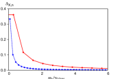
Figure S1: Gap function of the electron pocket $\bar{\Delta}_{X,n}$ as function of Matsubara frequency $\omega_{n}$ (in units of $\gamma_{\mathrm{SDW}}$) for the parameters used in the main text and $\xi_{\mathrm{Neel}}=0$ (red/solid line) and $\xi_{\mathrm{Neel}}=0.5a$ (blue/dashed line).

We see that the logarithmic derivative of the transition temperature (S47) is determined by the frequency dependence of the gap function (eigenvectors) $\bar{\Delta}_{i,n}$ – explicitly in the expectation value of $\delta\hat{K}_{s}$ and implicitly in the temperature dependence of $\eta$. In figure S1, we plot the gap $\bar{\Delta}_{X,n}$ of the electron pocket for the cases $\xi_{\mathrm{Neel}}=0$ (red/solid line) and $\xi_{\mathrm{Neel}}=0.5a$ (blue/dashed line). The hole pocket gap displays a similar behavior. Clearly, the s-wave gap in the presence of Neel fluctuations decreases much faster as function of frequency than the gap of the “pure” $s^{+-}$ state. Thus, the $s^{+-}$ state adapts to the presence of $\left(\pi,\pi\right)$ fluctuations by suppressing the gap at higher frequencies to avoid the main depairing effect, which comes from the high frequency components of the Neel spectrum.

IV Dependence of transition temperature on Impurity Scattering

The Bergmann-Rainer approach is also used to obtain the dependence of the transition temperature on impurity scattering:

$$\frac{\partial T_{c}^{\mathrm{s-wave}}}{\partial\tau^{-1}}=\left[\hat{\Delta}\frac{\partial\hat{K}_{s}}{\partial\tau^{-1}}\hat{\Delta}\right]_{\eta=0}/\left(-\frac{\partial\eta}{\partial T}\right)_{\eta=0}$$ (S48)

where $\tau^{-1}$ is the scattering rate due to impurity scattering. The reduced $\tilde{T}_{c}^{\mathrm{s-wave}}$ is then obtained via the linear approximation $\tilde{T}_{c}^{\mathrm{s-wave}}=T_{c}^{\mathrm{s-wave}}+\tau^{-1}\left(\frac{\partial T_{c}^{\mathrm{s-wave}}}{\partial\tau^{-1}}\right)$.

References

(1) K. Ishida, Y. Nakai and H. Hosono, J. Phys. Soc.
Japan 78, 062001 (2009); D. C. Johnston, Adv. Phys. 59,
803 (2010); J. Paglione and R. L. Greene, Nature Phys. 6,
645 (2010); P. C. Canfield and S. L. Bud’ko, Annu. Rev. Cond. Mat.
Phys. 1, 27 (2010); H. H. Wen and S. Li, Annu. Rev. Cond.
Mat. Phys. 2, 121 (2011).
(2) I. I. Mazin, D. J. Singh, M. D. Johannes, and
M. H. Du, Phys. Rev. Lett. 101, 057003 (2008); A. V. Chubukov,
D. V. Efremov and I Eremin, Phys. Rev. B 78, 134512 (2008);
K. Kuroki, S. Onari, R. Arita, H. Usui, Y. Tanaka, H. Kontani, and
H. Aoki, Phys. Rev. Lett. 101, 087004 (2008); V. Cvetković
and Z. Tešanović, Phys. Rev. B 80, 024512 (2009); J.
Zhang, R. Sknepnek, R. M. Fernandes, and J. Schmalian, Phys. Rev.
B 79, 220502(R) (2009); A. F. Kemper, T. A. Maier, S. Graser,
H-P. Cheng, P. J. Hirschfeld and D. J. Scalapino, New J. Phys. 12,
073030 (2010)
(3) P. J. Hirschfeld, M. M. Korshunov, and
I. I. Mazin, Rep. Prog. Phys. 74, 124508 (2011); A. V. Chubukov,
Annu. Rev. Cond. Mat. Phys. 3, 57 (2012).
(4) K. Kuroki, H. Usui, S. Onari, R. Arita, and H.
Aoki, Phys. Rev. B 79, 224511 (2009).
(5) M. D. Johannes and I. Mazin, Phys. Rev. B 79,
220510(R) (2009).
(6) M.J. Calderon, G. Leon, B. Valenzuela, and E.
Bascones, arXiv:1107.2279
(7) S. Graser, A. F. Kemper, T. A. Maier, H.-P. Cheng,
P. J. Hirschfeld, and D. J. Scalapino, Phys. Rev. B 81, 214503
(2010).
(8) G. S. Tucker, D. K. Pratt, M. G. Kim, S. Ran,
A. Thaler, G. E. Granroth, K. Marty, W. Tian, J. L. Zarestky, M. D.
Lumsden, S. L. Bud’ko, P. C. Canfield, A. Kreyssig, A. I. Goldman,
and R. J. McQueeney, arXiv:1206.3486
(9) Y. Texier, Y. Laplace, P. Mendels, J. T. Park, G.
Friemel, D. L. Sun, D. S. Inosov, C. T. Lin, J. Bobroff, EPL 99,
17002 (2012).
(10) A. S. Sefat, D. J. Singh, L. H. VanBebber,
Y. Mozharivskyj, M. A. McGuire, R. Jin, B. C. Sales, V. Keppens, and
D. Mandrus, Phys. Rev. B 79, 224524 (2009); J. S. Kim, S. Khim, H.
J. Kim, M. J. Eom, J. M. Law, R. K. Kremer, J. H. Shim, and K. H.
Kim, Phys. Rev. B 82, 024510 (2010); M. G. Kim, A. Kreyssig,
A. Thaler, D. K. Pratt, W. Tian, J. L. Zarestky, M. A. Green, S. L.
Bud’ko, P. C. Canfield, R. J. McQueeney, and A. I. Goldman, Phys.
Rev. B 82, 220503(R) (2010); K. Marty, A. D. Christianson,
C. H. Wang, M. Matsuda, H. Cao, L. H. VanBebber, J. L. Zarestky, D.
J. Singh, A. S. Sefat, and M. D. Lumsden, Phys. Rev. B 83,
060509(R) (2011); A. Pandey, V. K. Anand, and D. C. Johnston, Phys.
Rev. B 84, 014405 (2011); A. S. Sefat, K. Marty, A. D. Christianson,
B. Saparov, M. A. McGuire, M. D. Lumsden, W. Tian, and B. C. Sales,
Phys. Rev. B 85, 024503 (2012); A. Pandey, R. S. Dhaka, J.
Lamsal, Y. Lee, V. K. Anand, A. Kreyssig, T. W. Heitmann, R. J. McQueeney,
A. I. Goldman, B. N. Harmon, A. Kaminski, and D. C. Johnston, Phys.
Rev. Lett. 108, 087005 (2012).
(11) A. Thaler, H. Hodovanets, M. S. Torikachvili,
S. Ran, A. Kracher, W. Straszheim, J. Q. Yan, E. Mun, and P. C. Canfield,
Phys. Rev. B 84, 144528 (2011).
(12) P. C. Canfield, S. L. Bud’ko,
Ni Ni, J. Q. Yan, and A. Kracher, Phys. Rev. B 80, 060501(R)
(2009); N. Ni, A. Thaler, A. Kracher, J. Q. Yan, S. L. Bud’ko, and
P. C. Canfield, Phys. Rev. B 80, 024511 (2009);N. Ni, A.
Thaler, J. Q. Yan, A. Kracher, E. Colombier, S. L. Bud’ko, and P.
C. Canfield, Phys. Rev. B 82, 024519 (2010).
(13) J. Guo, S. Jin, G. Wang, S. Wang, K. Zhu, T. Zhou,
M. He, and X. Chen, Phys. Rev. B 82, 180520(R) (2010).
(14) T. A. Maier, S. Graser, P. J. Hirschfeld, and
D. J. Scalapino, Phys. Rev. B 83, 100515(R) (2011); T. A.
Maier, P. J. Hirschfeld, and D. J. Scalapino, arXiv:1206.5235.
(15) T. Das and A. V. Balatsky, arXiv:1208.2468
(16) G. M. Eliashberg, Sov. Phys. JETP 11,
696 (1960); Sov. Phys. JETP 16, 780 (1963).
(17) see J. P. Carbotte, Rev. Mod. Phys. 62,
1027 (1990) and references therein.
(18) P. Monthoux and D. Pines, Phys. Rev. Lett. 69,
961 (1992).
(19) A. J. Millis, Phys. Rev. B 45, 13047
(1992).
(20) Ar. Abanov, A. V. Chubukov, and A. M.
Finkel’stein, EPL 54, 488 (2001); Ar. Abanov, A. V. Chubukov,
and J. Schmalian, EPL 55, 369 (2001); Ar. Abanov, A. V. Chubukov,
and J. Schmalian, Adv. Phys. 52, 119 (2003); A. V. Chubukov
and J. Schmalian, Phys. Rev. B 72, 174520 (2005).
(21) R. Roussev and A. J. Millis, Phys. Rev. B 63,
140504(R) (2001).
(22) O. V. Dolgov, I. I. Mazin, D. Parker,
and A. A. Golubov, Phys. Rev. B 79, 060502(R) (2009); L.
Benfatto, E. Cappelluti, and C. Castellani, Phys. Rev. B 80,
214522 (2009); G. A. Ummarino, M. Tortello, D. Daghero, and R. S.
Gonnelli, Phys. Rev. B 80, 172503 (2009).
(23) V. Stanev and Z. Tešanović, Phys. Rev. B 81,
134522 (2010).
(24) R. Thomale, C. Platt, W. Hanke, J. Hu, and B.
A. Bernevig, Phys. Rev. Lett. 107, 117001 (2011); C. Platt,
R. Thomale, C. Honerkamp, S.-C. Zhang, and W. Hanke, Phys. Rev. B
85, 180502(R) (2012); M. Khodas and A. V. Chubukov, Phys.
Rev. Lett. 108, 247003 (2012).
(25) A. J. Millis, S. Sachdev, and C. M. Varma, Phys.
Rev. B 37, 4975 (1988).
(26) D. J. Bergmann and D. Rainer, Z. Phys.
263, 59 (1973).
(27) S. Maiti, M. M. Korshunov, T. A. Maier, P. J. Hirschfeld,
and A. V. Chubukov, Phys. Rev. B 84, 224505 (2011); ibid
Phys. Rev. Lett. 107, 147002 (2011).
(28) Y. Wang, J.S. Kim, G. R. Stewart, P.J. Hirschfeld,
S. Graser, S. Kasahara, T. Terashima, Y. Matsuda, T. Shibauchi, and
I. Vekhter, Phys. Rev. B 84, 184524 (2011).
(29) D. S. Inosov, J. T. Park, P. Bourges, D.
L. Sun, Y. Sidis, A. Schneidewind, K. Hradil, D. Haug, C. T. Lin,
B. Keimer, and V. Hinkov, Nature Phys. 6, 178 (2010); H.-F.
Li, C. Broholm, D. Vaknin, R. M. Fernandes, D. L. Abernathy, M. B.
Stone, D. K. Pratt, W. Tian, Y. Qiu, N. Ni, S. O. Diallo, J. L. Zarestky,
S. L. Bud’ko, P. C. Canfield, and R. J. McQueeney, Phys. Rev. B 82,
140503(R) (2010).
(30) L. Benfatto and E. Cappelluti, Phys. Rev. B
83, 104516 (2011).
(31) I. I. Mazin and J. Schmalian, Physica C
469, 614 (2009).
(32) R. M. Fernandes, D. K. Pratt, W. Tian, J.
Zarestky, A. Kreyssig, S. Nandi, M. G. Kim, A. Thaler, N. Ni, P. C.
Canfield, R. J. McQueeney, J. Schmalian, and A. I. Goldman, Phys.
Rev. B 81, 140501(R) (2010); R. M. Fernandes and J. Schmalian,
Phys. Rev. B 82, 014521 (2010).
(33) A. B. Vorontsov, M. G. Vavilov, and A. V. Chubukov,
Phys. Rev. B 79, 060508(R) (2009).
(34) M. Xu, Q. Q. Ge, R. Peng, Z. R. Ye, Juan Jiang,
F. Chen, X. P. Shen, B. P. Xie, Y. Zhang, and D. L. Feng, Phys. Rev.
B 85, 220504(R) (2012).
(35) J. T. Park, G. Friemel, Yuan Li, J.-H. Kim,
V. Tsurkan, J. Deisen- hofer, H.-A. Krug von Nidda, A. Loidl, A. Ivanov,
B. Keimer, D. S. Inosov, Phys. Rev. Lett. 107, 177005 (2011);
G. Friemel, J. T. Park, T. A. Maier, V. Tsurkan, Yuan Li, J. Deisen-
hofer, H.-A. Krug von Nidda, A. Loidl, A. Ivanov, B. Keimer, D. S.
Inosov, Phys. Rev. B 85, 140511(R) (2012).
(36) L. Sun et al., Nature 483, 67
(2012).
(37) F. Kretzschmar et al., arXiv:1208.5006.
(38) R. M. Fernandes, A. V. Chubukov, J. Knolle,
I. Eremin, and J. Schmalian, Phys. Rev. B 85, 024534 (2012).
(39) S. Kasahara, H. J. Shi, K. Hashimoto, S. Tonegawa,
Y. Mizukami, T. Shibauchi, K. Sugimoto, T. Fukuda, T. Terashima, A.
H. Nevidomskyy, and Y. Matsuda, Nature 486, 382 (2012).
(40) H.-H. Kuo, J. G. Analytis, J.-H. Chu, R. M. Fernandes,
J. Schmalian, and I. R. Fisher, arXiv:1207.3858.
(41) A. Bardasis and J. R. Schrieffer, Phys.
Rev. 121, 1050 (1961); D. J. Scalapino and T. P. Devereaux,
Phys. Rev. B 80, 140512(R) (2009).

References

(1) P. Monthoux and G. G. Lonzarich, Phys. Rev.
B 59, 14598 (1999).
(2) L. Benfatto and E. Cappelluti, Phys. Rev.
B 83, 104516 (2011).
(3) A. V. Chubukov and J. Schmalian, Phys. Rev.
B 72, 174520 (2005).
(4) see J. P. Carbotte, Rev. Mod. Phys. 62,
1027 (1990) and references therein.
(5) S. Graser, T. A. Maier, P. J. Hirschfeld, and
D. J. Scalapino, New J. Phys. 11, 025016 (2009).
(6) J. Zhang, R. Sknepnek, R. M. Fernandes, and J.
Schmalian, Phys. Rev. B 79, 220502(R) (2009).
(7) S. Maiti, M. M. Korshunov, T. A. Maier, P. J. Hirschfeld,
and A. V. Chubukov, Phys. Rev. Lett. 107, 147002 (2011).
(8) D. J. Bergmann and D. Rainer, Z. Phys.
263, 59 (1973).