Magnetic field reversals and galactic dynamos

Abstract

We argue that global magnetic field reversals similar to those observed in the Milky Way occur quite frequently in mean-field galactic dynamo models that have relatively strong, random, seed magnetic fields that are localized in discrete regions. The number of reversals decreases to zero with reduction of the seed strength, efficiency of the galactic dynamo and size of the spots of the seed field. A systematic observational search for magnetic field reversals in a representative sample of spiral galaxies promises to give valuable information concerning seed magnetic fields and, in this way, to clarify the initial stages of galactic magnetic field evolution.

Keywords: Galactic dynamos; Magnetic fields of galaxies; Magnetic field reversals; MHD

1 Introduction

An outstanding question in the study of magnetic fields in spiral galaxies is that of large-scale field reversals. Do they occur, how easily can they be detected, can dynamo models explain them?

It appears that there may be such a field reversal in the Milky Way – certainly there is a localized feature relatively close to the Sun, but the difficulties of observing through the confusion of the disc plane make it difficult to be absolutely certain whether it is global in extent. Further reversals have been claimed to exist, but with increasing uncertainty (e.g. Simard-Normandin and Kronberg, 1979; Beck et al., 1996; Frick et al., 2001; Men et al., 2008; Nota and Katgert, 2010; Pshirkov et al., 2011; van Eck et al., 2011; Beck, 2011). Speaking generally, the idea that magnetic field reversals are present in the Milky Way is widely accepted.

The situation in external galaxies (see the review Beck et al., 1996), where the problem of observing from a position in the disc plane is absent, is nevertheless rather more uncertain. Except for the immediate neighbours of the Milky Way, the available resolution is too low to make definitive statements. But in the well observed nearby M31, reversals appear to be absent.

Classical mean-field dynamo models that start from a dynamically small field do not in general produce field reversals (e.g. Ruzmaikin et al., 1988; Meinel et al., 1990), because the leading eigenfunction of the kinematic mean-field galactic dynamo usually has no reversals, and this dominates the field structure as the field strength grows.

The situation becomes less straightforward when the seed field for the dynamo is stronger in comparison to the contemporary galactic magnetic field, so the galactic dynamo becomes nonlinear before the magnetic field configuration approaches the leading eigenfunction of the kinematic dynamo. It appears that long-lived reversals can survive in the form of nonlinear fronts (Poezd et al., 1993; Beck et al., 1994; Moss et al., 1998): these are essentially field discontinuities, (see e.g. Belyanin et al., 1994; Vasil’eva et al., 1994; Moss et al., 2000; Petrov et al., 2001). However these models depend on rather carefully chosen initial conditions, and existing examples are one dimensional.

More recently, Moss et al. (2012) have published an extended mean-field model in which long-lived reversals appear to be a quite common feature. This dynamo model differs in several important ways from earlier 2D mean-field models. Notably these computations begin from initial conditions of small-scale, approximately equipartition strength, fields that are randomly distributed in many discrete spots. This is in contrast to nearly all previous mean-field models, which begin from dynamically weak seed fields, either quasi-homogeneous or small-scale. The rationale is that these dynamically strong fields are the result of small-scale dynamo action in star forming regions in the protogalaxy. In the computations described in Moss et al. (2012) there are also ongoing injections of small-scale field, but we will argue here that these are not central to the generation of reversals.

Our approach is close to that of the one dimensional model of Beck et al. (1994), where a localized random initial condition was considered and long-lived large-scale magnetic reversals developed. (This contrasts with the model of Poezd et al. (1993), where there were ongoing injections of random fields.) Thus both Poezd et al. (1993) and Beck et al. (1994) considered magnetic fields depending on galactocentric radius only, i.e. ring-like magnetic structures were described. The novelty of our approach is that we consider seed fields that depend on both radius and azimuth, i.e. there is no a priori restriction to ring-like structures, and any such structures develop as a result of the dynamo process. We demonstrate below that ring-like structures with reversals, similar to those described by Beck et al. (1994), also develop in our simulations. Thus our model reinforces and extends the results of Beck et al. (1994).

On the other hand, we note that the stable magnetic ring-like structures with reversals obtained by Poezd et al. (1993) appeared in a model with some fine tuning of the model parameters. Stability conditions for such structures obtained by Belyanin et al. (1994) depend on rather subtle properties of the galactic disc; this gave a hint that the magnetic configuration of the Milky Way with field reversals is a rare exception to the typical situation without reversals. Possibly, there was a misinterpretation of the results, and maybe the authors of the papers cited above were not insistent enough. Nevertheless, dynamo generated configurations with reversals remained rather neglected by the astronomical community. Moreover, the option of including continuous injection of small-scale magnetic field as considered by Poezd et al. (1993), was not further developed until recently.

In contrast, the new generation of dynamo models presented in Moss et al. (2012) produce magnetic structures with reversals even for the simplest and most primitive distribution of the dynamo governing parameters and they appear to occur more or less as commonly as structures without reversals. This is why we consider below examples of dynamo models with (and without) reversals. They are demonstrably oversimplified and do not include any fine tuning of the governing parameters of the dynamo.

The paper Moss et al. (2012) focussed on applications of the model to future observations of magnetic fields of the earliest galaxies using the recently developed (e.g. LOFAR) and planned (SKA) radio telescopes. The aim of this paper is to describe the long-lived reversals obtained as a quite general phenomenon of galactic dynamos. We are motivated here by future observations of magnetic fields in very young galaxies, whose detailed structures are almost unknown at the moment, and so we study a very simple, generic model. This is in some contrast to the approch of Poezd et al. (1993) (and to some extent Beck et al. (1994)) who focussed their attention on the dynamo properties of particular nearby galaxies (M31 and the Milky Way) and exploited particular subtle properties of their rotation curves and other parameters.

2 The dynamo model

Detailed modeling of galactic magnetic of galactic magnetic field evolution from the time of galactic formation up to the age of a contemporary galaxy is a severe problem, both because of obvious numerical difficulties and our very poor knowledge of hydrodynamics of early galaxies. Moss et al. (2012) used a reasonable simplification of the problem in the mean-field approach in the form of the ”no-$z$” model (e.g. Moss, 1995) which restricts the modelling to quantities which are accessible observationally, at least in the immediate future, and make the numerical implementation affordable. Phillips (2001) systematically compared this approximation with the standard ”local model” (cf. Ruzmaikin et al., 1988) and found satisfactory agreement.

Here we use the same simplified model. For the sake of clarity we briefly reproduce the relevant equations from Moss et al. (2012). The code solves in the $\alpha\omega$ approximation explicitly for the field components parallel to the disc plane while the component perpendicular to this plane (i.e. in the $z$-direction) is given by the solenoidality condition. An even (quadrupole-like) magnetic field parity with respect to the disc plane is assumed. The field components parallel to the plane can be considered as mid-plane values, or as a form of vertical average through the disc. The key parameters are the aspect ratio $\lambda=h/R$, where $h$ corresponds to the semi-thickness of the warm gas disc and $R$ is its radius, and the dynamo numbers $R_{\alpha}=\alpha_{0}h/\eta,R_{\omega}={\varOmega}_{0}h^{2}/\eta$ (if disc thickness varies with radius then $h$ is some reference value, $h_{0}$ say). $\lambda$ must be a small parameter. $\eta$ is the turbulent diffusivity, assumed uniform, and $\alpha_{0},{\varOmega}_{0}$ are typical values of the $\alpha$-coefficient and angular velocity respectively. Thus the dynamo equations become in cylindrical polar coordinates $(r,\phi,z)$

$$\frac{\partial B_{r}}{\partial t}=-R_{\alpha}B_{\phi}-\frac{\pi^{2}}{4}B_{r}+\lambda^{2}\left[\frac{\partial}{\partial r}\left(\frac{1}{r}\frac{\partial}{\partial r}(rB_{r})\right)+\frac{1}{r^{2}}\frac{\partial^{2}B_{r}}{\partial\phi^{2}}-\frac{2}{r^{2}}\frac{\partial B_{\phi}}{\partial\phi}\right],$$ (1)

$$\frac{\partial B_{\phi}}{\partial t}=R_{\omega}rB_{r}\frac{{\mathrm{d}}{\varOmega}}{{\mathrm{d}}r}-R_{\omega}{\varOmega}\frac{\partial B_{\phi}}{\partial\phi}-\frac{\pi^{2}}{4}B_{\phi}+\lambda^{2}\left[\frac{\partial}{\partial r}\left(\frac{1}{r}\frac{\partial}{\partial r}(rB_{\phi})\right)+\frac{1}{r^{2}}\frac{\partial^{2}B_{\phi}}{\partial\phi^{2}}-\frac{2}{r^{2}}\frac{\partial B_{r}}{\partial\phi}\right],$$ (2)

where $z$ does not appear explicitly. Here the disc semi-thickness $h$ is assumed to be constant: taking $h=h(r)$ would introduce geometric correction factors $(h(r)/h_{0}),(h(r)/h_{0})^{2}$ multiplying $R_{\alpha}$, and the terms $-\frac{\pi^{2}}{4}(B_{r},B_{\phi})$, respectively. This equation has been calibrated by introduction of the factors $\pi^{2}/4$ in the vertical diffusion terms. In principle in the $\alpha\omega$ approximation the parameters $R_{\alpha},R_{\omega}$ can be combined into a single dynamo number $D=R_{\alpha}R_{\omega}$, but we choose to keep them separate. Equations (1) and (2) are displayed in polar coordinates but for ease of numerical implementation they are rewritten in Cartesians. Computations are performed on a uniform grid of resolution $229\times 229$ in the region $-1\leq x,y\leq 1$. This resolution was tested in Moss et al. (2012), and indeed is in excess of what is required for the very straightforward dynamo problem solved after $t=0$. The unit of time is about $0.8$ Gyr. Further details are given in Moss et al. (2012).

Length, time and magnetic field are non-dimensionalized in units of $R$, $h^{2}/\eta$ and the equipartition field strength $B_{\rm eq}$ respectively. A naive algebraic $\alpha$-quenching nonlinearity is assumed, $\alpha=\alpha_{0}/(1+B^{2}/B_{\rm eq}^{2})$, where $B_{\rm eq}$ is the strength of the equipartition field in the general disc environment. Note that small-scale field is injected only at time zero; after that we conduct a standard mean field dynamo simulation.

The coefficients $\alpha_{0}$ and $B_{\rm eq}$ are assumed to be uniform in the work described in this paper because our restricted knowledge of the properties of the earliest galaxies give no secure basis for more realistic assumptions. For example, it is argued that $\alpha_{0}$ depends on both disc thickness and local angular velocity, i.e. $\alpha_{0}\propto{\varOmega}h^{-1}$, where $h$ can be expected to increase with radius, and ${\varOmega}$ to decrease. Of course, we continue our simulations to a time corresponding to the present day where knowledge of particular galaxies is rather better – we emphasize again that we are studying generic properties of thin disc dynamos. Taking typical galactic values, we can estimate $R_{\alpha}={\mathrm{O}}(1)$, $R_{\omega}={\mathrm{O}}(10)$ (i.e. $D={\mathrm{O}}(10)$).

We appreciate that more sophisticated approaches to the saturation process exist, however it does appear that in some cases at least, such a naive algebraic quenching can reproduce reasonably well the results from a more sophisticated treatment (e.g. Kleeorin et al., 2002).

3 Results

Moss et al. (2012) presented a particular galactic dynamo model that quite often resulted in magnetic field configuration with one or more reversals. We argue here that many specific features of the model Moss et al. (2012) are not essential for the development of reversals.

We show in figure 2a the statistically steady field (at age ca. 13 Gyr) resulting from a standard computation of Moss et al. (2012) (model 135, $R_{\alpha}=1,R_{\omega}=20$; we keep here and below the numbers of the models from the working journal to allow identification of the models between various papers). In this case the initial field is randomly distributed in $n_{\rm spot}=100$ discrete regions, with r.m.s. value $B_{0}$ of the field in these regions of order unity - i.e. the alpha-quenching nonlinearity is immediately important. Figure 1 shows a representation of this initial field. Large-scale reversals are clearly visible in the resulting statistically steady configuration of this model – figure 2a. We then show in figure 2b (model NOINJECT10) the results of a similar computation using the same initial conditions, the only difference being that there is now no ongoing injection of fields in discrete regions. The final, steady, field is now smooth (the irregularities visible in figure 2a are caused by the ongoing injection of small-scale field), but two large-scale reversals are again clearly visible. A reversal has appeared by dimensionless time $t=1$ (age $\;\raise 1.29167pt\hbox{$<$\kern-7.5pt\raise-4.73611pt\hbox{$\sim$ }}\;\hskip-2.0pt1$ Gyr), and have stabilized by $t=3$ (ca $2.5$ Gyr). A time sequence is shown in figure 3 for the model whose steady configuration is shown in figure 2b.

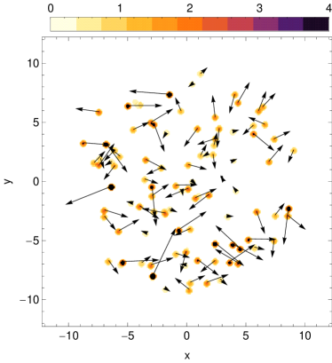
Figure 1: (Colour online). A typical configuration of the initial magnetic field; only the ${\bm B}$ vectors at the centre of the spots are shown. The shaded circles indicate the gaussian half-width of the spots. (Taken from Moss et al. (2012).)

We expect that by reducing the strength of the seed field we will reduce the number of reversals to zero. In order to test this prediction we repeated the computation of figure 2b with the r.m.s. value, $B_{0}$, of the initial field in the discrete spots that was smaller by a factor of $10^{-6}$, and then by a factor of $10^{-8}$. In the first of these cases the steady configuration has a single reversal (figure 4a, model NOINJECT11), in the second case there are no reversals (figure 4c, model NOINJECT16).

(a)

(b)

Figure 2: (a) Statistically steady state of model 135 of Moss et al. (2012) with $R_{\alpha}=1,R_{\omega}=20$ at dimensionless time $t=17$ (approximately $13$ Gyr); (b) steady state of similar model without the ongoing injections of random field (NOINJECT10) at the same time.

(a)

(b)

(c)

Figure 3: Snapshots of the field configuration of the model NOINJECT10 at times (a) $t=0.1$ (ca. $0.08$ Gyr); (b) $t=1.0$ (ca. $0.8$ Gyr); (c) $t=3.0$ (ca. $2.4$ Gyr).

We also anticipate that a reduction of efficiency of the large-scale dynamo will affect reversals in a more or less similar way as reducing the seed field strength. The point is that both of these changes act to prolong the stage of quasi-kinematic magnetic field evolution. We verified this expectation, repeating the above computations with $R_{\omega}$ reduced from $20$ to $10$; then with $B_{0}\approx 1$ there is one reversal in the final steady configuration, and with $R_{\omega}=7$ there are no reversals. With $B_{0}\approx 10^{-6},R_{\omega}=20$ there are none.

(a)	(b)
(c)	(d)

Figure 4: Steady field configurations for (a) $R_{\alpha}=1,R_{\omega}=20$, r.m.s. value of initial spotty field $B_{0}\approx 10^{-6}$; (b) $R_{\alpha}=1,R_{\omega}=20$, initial field randomly assigned at every mesh point with r.m.s. value of unity; (c) as (a) with $B_{0}\approx 10^{-8}$; (d) the model NOINJECT10 with a different realization of random numbers – compare figure 2b.

If the size of the spots that localize the seed field becomes very small, reversals disappear. We demonstrate this in an experiment where the initial field is randomly assigned at every mesh point, again with $R_{\alpha}=1,R_{\omega}=20$, and $B_{0}\approx 1$. The final steady field configuration is shown in figure 4b (model NOINJECT12) – it is smooth with no reversals. A similar result was found with $B_{0}\approx 10^{-6}$. Note that, in order to simplify comparison between these models, we used the same realization of random numbers to determine the seed field distribution in each case discussed above, with the exception of the case shown in figure 4b.

We further show that the eventual steady state configuration has some dependence on the initial conditions, by the following experiment. The case NOINJECT10 (the same initial conditions as model 135 from Moss et al. (2012), without the ongoing field injections) is re-simulated with a different realization of the random numbers, arriving at a field configuration that is quite different from that shown in figure 2b – see figure 4d. We also repeated the NOINJECT10 calculation with ‘global’ alpha-quenching, i.e. quenching by the mean global energy. The final configuration was quite different, but reversals are again present. We conclude that the form of the initial field can influence significantly the steady state configuration.

Repeating the case illustrated in figure 2b with $n_{\rm spot}=50$ produces a superficially quite similar final state. As a final check, a simulation with $n_{\rm spot}=1,B_{0}=1$ produces a field without reversals.

4 Discussion and Conclusions

We deduce from these experiments that long-lived reversals can be generated by a standard 2D (nonaxisymmetric) mean-field dynamo model, given suitable initial conditions and a suitable range of the dynamo governing parameters. The initial conditions play a key role – this is probably why such solutions have not been widely noted previously. Different steady solutions can be found for the same dynamo parameters, depending on the initial conditions. Large-scale reversals can appear after about $1$ Gyr, and they stabilize after $2-3$ Gyr. The important elements appear to be an inhomogeneous distribution of the initial field and strong differential rotation (larger $R_{\omega}$), the latter effect being enhanced by initial fields that are locally near equipartition values. Note that even with larger values of $R_{\omega}$ ($R_{\omega}=20$ say), some initial conditions still produce final configurations without reversals.

We note that some of these results were anticipated by Beck et al. (1994). This paper studied a one-dimensional model and showed that, with a sufficiently strong small-scale seed field, reversals could persist for times of order the age of the Universe.

As a straightforward consequence of the above conclusion, a systematic observational search for magnetic field reversals in a representative sample of spiral galaxies may provide valuable information concerning seed magnetic fields, and so clarify initial stages of galactic magnetic field evolution. This appears to be a realistic possibility for the forthcoming generation of radio telescopes. For a contemporary comparison, it might be appropriate for orientation to look at figure 11 of van Eck et al. (2011), showing their best model of the reversals in the Milky Way field.

If we compare figure 2a with subsequent plots, the ongoing magnetic field injections gives an important additional mechanism to generate magnetic reversals. In addition to the global scale magnetic field reversals discussed above, this model contains several local reversals which appear to be due to local field injections, and which exist for some time. Possibly, such local reversals can be compared with reversals suggested to exist in the Milky Way (see e.g. Han and Zhang, 2007)

We appreciate that the models presented are very oversimplified, but our intention is to show that initial conditions can strongly influence the long term evolution of the large-scale magnetic field. With ”standard” weak initial fields ($|{\bm B}|<<B_{\rm eq}$), any reversals are transient features. It appears important that the nonlinearity operates before the large-scale field forms. Of course, confirmation or revision of the conclusions of this paper in the framework of 3D mean-field models, or even by direct numerical simulations of the microscopic induction equation, performed with realistic hydrodynamical models of very early galaxies would be an important development of the theory of galactic dynamos. However this obviously is beyond the scope of this paper.

We are grateful to our colleagues, who work on magnetic field evolution in very young galaxies namely T. Arshakian, R. Beck, M. Krause, R. Stepanov, for fruitful discussions which stimulated the writing of this the paper. We also thank Anvar Shukurov and an anonymous referee for critical readings of the paper.

References

- Beck et al. (1996) Beck, R., Brandenburg, A., Moss, D., Shukurov and Sokoloff, D., Galactic magnetism: Recent developments and perspectives. Ann. Rev. Astron. Astrophys. 1996, 34, 155–206.
- Beck et al. (1994) Beck, R., Poezd, A.D., Shukurov, A. and Sokoloff, D. D., Dynamos in evolving galaxies. Astron. Astrophys. 1994, 289, 94–100.
- Beck (2011) Beck, R., Cosmic Magnetic Fields: Observations and Prospects, arXiv 1104.3479, 2011.
- Belyanin et al. (1994) Belyanin, M.P., Sokoloff, D.D. and Shukurov, A.M., Asymptotic steady-state solutions to the nonlinear hydromagnetic dynamo equations. Russ. J. Math. Phys. 1994, 2, 149-174. 155–206.
- Frick et al. (2001) Frick, P., Stepanov, R., Shukurov, A., Sokoloff, D., Structures in the rotation measure sky, Mon. Not. Roy. Astron. Soc. 2001, 325, 649-664.
- Han and Zhang (2007) Han, J.L. and Zhang, J.S., The Galactic distribution of magnetic fields in molecular clouds and HII regions, Astron. Astrophys. 2007, 464, 609-614.
- Kleeorin et al. (2002) Kleeorin, N., Moss, D., Rogachevskii, I. and Sokoloff, D., The role of magnetic helicity transport in nonlinear galactic dynamos. Astron. Astrophys. 2002, 387, 453-462.
- Meinel et al. (1990) Meinel, R., Elstner, D. and Ruediger, G., The galactic dynamo in perfectly conducting surroundings. Astron. Astrophys. 1990, 236, L33-L35.
- Men et al. (2008) Men, H., Ferrière, K., and Han, J.L., Observational constraints on models for the interstellar magnetic field. Astron. Astrophys. 2008, 486, 819-828.
- Moss (1995) Moss, D., On the generation of bisymmetric magnetic field structures in spiral galaxies by tidal interactions. Mon. Not. Roy. Astron. Soc. 1995, 275, 191–194.
- Moss et al. (2012) Moss, D., Stepanov, R., Arshakian, T.G., Beck, R., Krause, M. and Sokoloff, D., Multiscale magnetic fields in spiral galaxies: evolution and reversals. Astron. Astrophys. 2012, 537, A68 .
- Moss et al. (2000) Moss, D., Petrov, A. and Sokoloff, D., The motion of magnetic fronts in spiral galaxies. Geophys. Astrophys. Fluid Dyn. 2000, 92, 129-149.
- Moss et al. (1998) Moss, D., Shukurov, A. and Sokoloff, D., Boundary effects and propagating, magnetic fronts in disc dynamos, Geophys. Astrophys. Fluid Dyn. 1998, 89, 285-308.
- Nota and Katgert (2010) Nota, T. and Katgert, P., The large-scale magnetic field in the fourth Galactic quadrant. Astron. Astrophys. 2010, 513, A65.
- Petrov et al. (2001) Petrov, A.P., Sokoloff, D.D. and Moss, D.L., Magnetic fronts in galaxies. Astron. Rep. 2001, 45, 497-501.
- Poezd et al. (1993) Poezd, A., Shukurov, A. and Sokoloff, D., Global magnetic patterns in the Milky-Way and the Andromeda nebula. Mon. Not. Roy. Astron. Soc. 1993, 264, 285-297.
- Phillips (2001) Phillips, A.D., A comparison of the asymptotic and no-z approximations for galactic dynamos. Geophys. Astrophys. Fluid Dyn. 2001, 94, 135-150.
- Pshirkov et al. (2011) Pshirkov, M. S., Tinyakov, P.G., Kronberg, P.P. and Newton-McGee, K.J., Deriving the global structure of the Galactic magnetic field from Faraday rotation measures of extragalactic sources. Astrophys. J. 2011, 738, 192.
- Ruzmaikin et al. (1988) Ruzmaikin A.A., Shukurov, A.M. and Sokoloff, D.D.., Magnetic Fields of Galaxies, 1988, Kluwer, Dordrecht.
- Simard-Normandin and Kronberg (1979) Simard-Normandin, M. and Kronberg, P.P., New large-scale magnetic features of the Milky Way. Nature 1979, 279, 115–118.
- Vasil’eva et al. (1994) Vasil’eva, A., Nikitin, A. and Petrov, A., Stability of contrasting solutions of nonlinear hydromagnetic dynamo equations and magnetic fields reversals in galaxies. Geophys. Astrophys. Fluid Dyn. 1994, 78, 261-279.
- van Eck et al. (2011) van Eck, C.L., Brown, J.C., Stil, J.M., Rae, K., Mao, S.A., and 6 others, Modelling the magnetic field in the Galactic disk using new rotation measure observations from the Very Large Array. Astrophys. J. 2011, 728, 97