SN 2007bg: The Complex Circumstellar Environment Around One of the Most Radio-Luminous Broad-Lined Type Ic Supernovae

Abstract

In this paper we present the results of the radio light curve and X-ray observations of broad-lined Type Ic SN 2007bg. The light curve shows three distinct phases of spectral and temporal evolution, implying that the SNe shock likely encountered at least 3 different circumstellar medium regimes. We interpret this as the progenitor of SN 2007bg having at least two distinct mass-loss episodes (i.e., phases 1 and 3) during its final stages of evolution, yielding a highly-stratified circumstellar medium. Modelling the phase 1 light curve as a freely-expanding, synchrotron-emitting shell, self-absorbed by its own radiating electrons, requires a progenitor mass-loss rate of $\dot{M}\approx 1.9\times 10^{-6}(v_{w}/1000\;\rm{km\,s}^{-1})$ M${}_{\odot}\,$yr^-1 for the last $t\sim 20(v_{w}/1000\;\rm{km\,s}^{-1})$ yr before explosion, and a total energy of the radio emitting ejecta of $E\approx 1\times 10^{48}$ erg after $10$ days from explosion. This places SN 2007bg among the most energetic Type Ib/c events. We interpret the second phase as a sparser ”gap” region between the two winds stages. Phase 3 shows a second absorption turn-on before rising to a peak luminosity $2.6$ times higher than in phase 1. Assuming this luminosity jump is due to a circumstellar medium density enhancement from a faster previous mass-loss episode, we estimate that the phase 3 mass-loss rate could be as high as $\dot{M}\la 4.3\times 10^{-4}(v_{w}/1000\;\rm{km\,s}^{-1})$ M${}_{\odot}\,$yr^-1. The phase 3 wind would have transitioned directly into the phase 1 wind for a wind speed difference of $\approx 2$. In summary, the radio light curve provides robust evidence for dramatic global changes in at least some Ic-BL progenitors just prior ($\sim 10-1000$ yr) to explosion. The observed luminosity of this SN is the highest observed for a non-gamma-ray-burst broad-lined Type Ic SN, reaching $L_{8.46\,\rm{GHz}}\approx 1\times 10^{29}$ erg Hz^-1 s^-1, $\sim 567$ days after explosion.

1 Introduction

Core collapse supernovae (SNe) mark the spectacular death of massive stars (Woosley & Weaver, 1986). Among these SNe Types Ib and Ic (collectively referred to as Ib/c due to their perceived similarities) are associated with the explosion of massive stars which were stripped of their H envelopes by strong stellar winds. Types Ib show He features in their spectra, whereas Types Ic do not. Our current understanding of Type Ib/c SNe suggests that Wolf-Rayet (WR) stars are a primary progenitor path (Van Dyk, Li & Filippenko, 2003), although the relative numbers of WR stars fall well short of the observed Type Ib/c rates and thus a lower-mass binary progenitor path is most likely required to account for a significant fraction of these events (e.g., Podsiadlowski et al., 1992; Ryder et al., 2004; Weiler et al., 2011; Smith et al., 2011). Archival imaging of pre-SNe locations, however, have failed to produce direct associations between Type Ib/c SNe and their possible progenitors (e.g., Smartt, 2009). Thus we must rely both on theory and indirect information obtained after the explosion. Fortunately, X-ray and radio emission are detectable by-products of the shock interaction between the high-velocity ejecta and the low-velocity progenitor wind in SNe (whereas the optical emission is generated by lower-velocity ejecta and radioactive decay). These observables crudely scale with the density of the circumstellar medium (CSM), and hence provide constraints on the wind properties of the SN progenitor (e.g., Chevalier, 1982a, b). Because massive stars are expected to have strong episodic mass-loss (e.g., Humphreys & Davidson, 1994) and line driven winds (e.g., Vink, de Koter & Lamers, 2000), radio monitoring of Type Ib/c SNe provide interesting constraints on possible progenitor types. The past decade has witnessed increased attention on Type Ib/c SNe due to the association of Type Ic SN 1998bw with gamma-ray burst (GRB) 980425 (Galama et al., 1998), as these objects may help elucidate how the central engines of both GRBs and their associated SNe work. Following this historic connection, several other Type Ic SNe have been linked to GRBs (e.g., Hjorth et al., 2003; Kawabata et al., 2003; Matheson et al., 2003; Stanek et al., 2003; Frail et al., 2005; Modjaz et al., 2006; Woosley & Bloom, 2006; Bufano et al., 2012); all of these objects show broad emission lines in their optical spectra, with velocities above $15000$ km s^-1. To date so far 5 GRBs have been spectroscopically confirmed to have a SNe counterpart, while 14 show photometric evidence of a SNe counterpart (Hjorth & Bloom, 2011), and hence a larger sample is needed in order to shed some light on the explosion mechanisms involved. Given the large number of SNe Type Ic compared to GRBs, one key question is whether these SNe could simply be off-axis GRBs. Initial efforts concluded that the vast majority were not (e.g., Soderberg et al., 2006c). Recently new evidence was presented for the detection of at least one possible off-axis GRB with no direct observation of the gamma-ray emission: SN 2009bb (Soderberg et al., 2010b); as well as the more controversial SN 2007gr (Paragi et al., 2010; Soderberg et al., 2010a; Xu et al., 2011).

Here we report on a particularly interesting broad-lined Type Ic, SN 2007bg, which was optically discovered on 2007 April 16.15 UT at $\alpha=11^{\rm h}49^{\rm m}26.18^{\rm s}$, $\delta=+51^{\circ}49^{\prime}21.8^{\prime\prime}$ (J2000) at redshift $z=0.0346$ (Quimby, Rykoff & Yuan, 2007) ($d=152$ Mpc, $H_{0}=70$ km s^-1 Mpc^-1, $\Omega_{\rm{M}}=0.3$, and $\Omega_{\rm{\Lambda}}=0.7$ in a $\Lambda$CDM cosmology). A spectrum taken on 2007 April 18.3 with the 9.2 m Hobby-Everly Telescope let Quimby et al. (2007) classify SN 2007bg as a Type Ic broad-lined (Ic-BL) supernova. The classification of this SN as a Type Ic and the fact that it resides in a faint host encouraged Prieto, Stanek & Beacom (2008) to think about this object as a likely off-axis GRB. Prieto, Watson & Stanek (2009) also noted that SN 2007bg was one of the brightest radio SNe one year after explosion, making it an even better candidate for an off-axis GRB. However, based on the radio light curve of SN 2007bg known at the time, Soderberg (2009) contended that the observed radio emission could be explained by the presence of a density enhancement in the CSM, rather than a GRB like central engine driving the explosion. Using the archival radio data for SN 2007bg, we further address this issue below.

The article outline is the following. In §2 we introduce the observations taken with the Very Large Array (VLA). Our results and modelling of the radio light curves are presented in §3. Finally in §4 we summarise our findings and provide a brief discussion on the future of radio observations of SNe.

2 Observations

2.1 Radio

The VLA radio observations were carried out between 2007 April 19 and 2009 August 28 as part of the programs AS887, AS929 and AS983 (PI A. M. Soderberg).

The data were taken in standard continuum observing mode, with a bandwidth of $2\times 50$ MHz. Data were collected at $1.43$, $4.86$, $8.46$, $15$, $22.5$ and $43.3$ GHz. As primary flux density calibrators 3C286 and 3C147 were used. We used these calibrators to scale our flux density measurements to the Perley-Buttler 2010 absolute flux scale. For secondary calibrators three different sources were used; SDSS J114856.56+525425.2 in most epochs, as well as SDSS J114644.20+535643.0 and SBS 1150+497. The derived flux density for the secondary calibrators is shown in Table 1. Traditionally one has been able to cross-check the derived secondary calibrator fluxes with archival data, but in this case the VLA stopped regular monitoring of calibrators since 2007. This, in combination with the weak calibrator for the $15$ and $22.5$ GHz data, makes this data less reliable than the rest at lower frequencies, even adopting larger error bars for it.

Table 1: VLA secondary calibrator measurements^a

Obs.	$f_{1.43\,\rm{GHz}}$	$f_{4.86\,\rm{GHz}}$	$f_{8.46\,\rm{GHz}}$	$f_{15\,\rm{GHz}}$	$f_{22.5\,\rm{GHz}}$
Date	(Jy)	(Jy)	(Jy)	(Jy)	(Jy)
2007-Apr-19			0.4525
2007-Apr-23			0.4306		0.2732
2007-Apr-24		0.4571	0.433
2007-Apr-25			0.453		0.282
2007-Apr-26		0.4552	0.4521	0.3644
2007-Apr-30		0.467	0.4583
2007-May-3				0.355	0.2752
2007-May-5		0.458	0.4427
2007-May-12		0.412	0.396	0.3607	0.2733
2007-May-17		0.4582	0.4623	0.3590	0.268
2007-May-27	0.4533b	0.4507	0.4173	0.345	0.2784
2007-Jun-11		0.45	0.464	0.359	0.2781
2007-Jun-22		0.4587	0.4372
2007-Jul-3				0.30	0.29
2007-Jul-7		0.4599	0.4479
2007-Jul-24	0.465b	0.453	0.4462	0.349	0.266
2007-Aug-18		0.4545	0.4410	0.348	0.2720
2007-Sep-7	0.465b	0.464	0.4475	0.352	0.30
2007-Sep-23	0.476b	0.4668	0.4624
2007-Oct-23	0.459b	0.4514	0.4410
2007-Nov-17	0.4562b	0.4332	0.4449
2007-Dec-23	0.452b	0.4583	0.4513
2008-Jan-3					0.2685
2008-Jan-28		0.50	0.475		0.10
2008-Feb-25		0.4642	0.4561		0.304
2008-Apr-19	0.476b	0.6247b	0.587b
2008-May-7			0.449
2008-Jun-9		1.197c	1.05c		1.050c
2008-Nov-3	0.5160b	0.6480b	0.6069b		0.491b
2008-Dec-30			0.481	0.351
2009-Apr-6	0.5100b	0.575b	0.5430b		0.3491b
2009-May-31	0.503b	0.5763b	0.523b
2009-Aug-27	0.530b	0.5411b	0.5162b
a Unless otherwise stated, the flux density measurements are
for SDSS J114856.56+525425.2.
b Flux density measurements are for SDSS J114644.20+535643.0.
c Flux density measurements are for SBS 1150+497.
On 2008 January 5 the source was observed at $43.3$ GHz.
The secondary calibrator flux during this epoch is $0.209$ Jy.

During this period of time, the VLA incorporated the new EVLA correlator to some of the antennas, so some of the antennas did not have all of the different wavelength receivers. This greatly reduced the sensitivity of observations during some epochs, especially at $1.43$ and $15$ GHz. We flagged, calibrated, and imaged the observations using the CASA (Common Astronomy Software Applications) software following standard procedures. We combined VLA and EVLA baselines, and to reduce the effects of the differences between VLA and EVLA antennas, we derived baseline-dependent calibrations on the primary flux calibrator.

To measure the flux density of the source we fitted a Gaussian at the source position in our cleaned images, as for upper limits these were computed from the dirty map rms in the central region. Since the rms noise in each cleaned map only provides a lower limit on the total error we added a systematic uncertainty $\epsilon_{\nu}$ due to possible inaccuracies of the VLA flux density calibration and deviations from an absolute flux density scale resulting in a final error for each flux density measurement of $\sigma^{2}=(\epsilon_{\nu}S_{\nu})^{2}+\sigma_{\it{rms}}^{2}$, with $\epsilon_{\nu}=0.2,0.2,0.1,0.05,0.05,0.05$ at $43.3$, $22.5$, $15$, $8.46$, $4.86$, and $1.43$ GHz. The factors were chosen based on the quality of the secondary calibrator, and on the observed phase scatter after calibration of the data. The resulting flux density measurements of SN 2007bg are shown in Table 2 along with the image rms.

Table 2: VLA flux density measurements for SN 2007bg

Obs.	$\Delta t$	$f_{1.43\,\rm{GHz}}$	$f_{4.86\,\rm{GHz}}$	$f_{8.46\,\rm{GHz}}$	$f_{15\,\rm{GHz}}$	$f_{22.5\,\rm{GHz}}$	$f_{43.3\,\rm{GHz}}$	Array
Date	(Days)a	($\mu$Jy)	($\mu$Jy)	($\mu$Jy)	($\mu$Jy)	($\mu$Jy)	($\mu$Jy)	Configuration
2007-Apr-19	2.9			$\leq$264				D
2007-Apr-23	7.0			$\leq$348		$\leq$1421		D
2007-Apr-24	7.8		$\leq$390	$\leq$387				D
2007-Apr-25	8.8			$\leq$417		1293 $\pm$ 220		D
2007-Apr-26	9.8		$\leq$339	$\leq$555	$\leq$666			D
2007-Apr-30	13.8		$\leq$291	480 $\pm$ 102				D
2007-May-03	16.8				$\leq$978	1032 $\pm$ 75		D
2007-May-05	19.2		$\leq$1692	753 $\pm$ 107				D
2007-May-12	26.1		$\leq$1905	804 $\pm$ 100	1900 $\pm$ 300	1062 $\pm$ 245		D
2007-May-17	30.9		$\leq$657	728 $\pm$ 87	1480 $\pm$ 289	$\leq$1050		D
2007-May-27	41.3	$\leq$171	487 $\pm$ 96	1257 $\pm$ 53	1250 $\pm$ 270	$\leq$1020		A
2007-Jun-11	55.9		$\leq$1191	1490 $\pm$ 104	2000 $\pm$ 308	1246 $\pm$ 127		A
2007-Jun-22	66.8		709 $\pm$ 60	1390 $\pm$ 45				A
2007-Jul-03	77.8				$\leq$843	$\leq$978		A
2007-Jul-07	81.8		915 $\pm$ 62	1325 $\pm$ 47				A
2007-Jul-24	98.8	$\leq$201	886 $\pm$ 80	1131 $\pm$ 59	$\leq$909	$\leq$870		A
2007-Aug-18	124.0		1050 $\pm$ 90	957 $\pm$ 64	$\leq$957	$\leq$693		A
2007-Sep-07	144.0	$\leq$336	1103 $\pm$ 88	621 $\pm$ 81	$\leq$1137	$\leq$825		A
2007-Sep-23	159.8	$\leq$525	792 $\pm$ 77	316 $\pm$ 57				AnB
2007-Oct-23	189.9	$\leq$585	685 $\pm$ 62	379 $\pm$ 59				AnB
2007-Nov-17	214.9	$\leq$342	479 $\pm$ 65	404 $\pm$ 62				B
2007-Dec-23	250.9	$\leq$387	685 $\pm$ 65	783 $\pm$ 57				B
2008-Jan-03	261.8					1723 $\pm$ 77		B
2008-Jan-05	263.8						$\leq$1662	B
2008-Jan-28	286.8		$\leq$594	1669 $\pm$ 90		$\leq$999		B
2008-Feb-25	314.8		1059 $\pm$ 70	2097 $\pm$ 73		2570 $\pm$ 160		CnB
2008-Apr-19	368.8	$\leq$822	1304 $\pm$ 62	2200 $\pm$ 59				C
2008-May-07	386.8			2852 $\pm$ 58				C
2008-Jun-09	419.9		2039 $\pm$ 88	3344 $\pm$ 81		2023 $\pm$ 140		DnC
2008-Nov-03	566.9	$\leq$321	2812 $\pm$ 60	3897 $\pm$ 78		1854 $\pm$ 128		A
2008-Dec-30	623.8			3891 $\pm$ 78	$\leq$2358			A
2009-Apr-06	720.8	746 $\pm$ 168	3390 $\pm$ 136	3842 $\pm$ 69		1629 $\pm$ 115		B
2009-May-31	775.8	$\leq$1167	3460 $\pm$ 80	3641 $\pm$ 79				CnB
2009-Aug-27	863.8	$\leq$1503	3373 $\pm$ 84	3408 $\pm$ 109				C
a Days since explosion assuming an explosion date of 2007 April 16.15 UT.
All upper limits are $3\sigma$.

2.2 X-Ray

SN 2007bg was observed seven times with the Swift X-ray Telescope (XRT) and once with the Chandra X-ray Observatory, as listed in Table 3. Processed data were retrieved from the Swift and Chandra archives, and analysis was performed using the HEASOFT (v6.12) and CIAO (v4.4.1) software packages, along with the latest calibration files available at the time. In the case of Chandra, we reprocessed the data to apply the latest calibration modifications, apply positional refinements, and correct for charge transfer inefficiency (CTI). All datasets were then screened for standard grade selection, exclusion of bad pixels and columns, and intervals of excessively high background (none was found).

The seven Swift datasets were combined into three rough epochs. We adopted a 35″radius aperture (corresponding to $\sim$85% encircled energy) as the source extraction region and modelled the local diffuse and scattered background using an annulus of 35–100″. No statistically significant detection was found within our adopted aperture. For the Chandra dataset, we adopted a 1$\aas@@fstack{\prime\prime}$5 radius aperture (corresponding to $\sim$95% encircled energy) as the source extraction region and modelled the local diffuse and scattered background using an annulus of 1.5–10″. Although five (5) counts fell within our aperture (a $\sim 2\sigma$ signal), no statistically significant detection could be made. Upper limits in all cases were determined using the Bayesian technique from Kraft, Burrows & Nousek (1991). We used PIMMS v4.6 to determine a count-to-flux conversion, adopting an absorbed APEC thermal plasma model with $kT=4$ keV and $N_{\rm{H}}=1.5\times 10^{20}$ cm^-2 (Dickey & Lockman, 1990).

Table 3: X-Ray measurements for SN 2007bg

Datea	Instrument	Obsid	Exposure	0.5-8.0	$F_{0.5-8.0}$	$L_{0.5-8.0}$
		(ks)		Counts	(erg s-1 cm-2)	(erg s-1)
2007-Apr-221	Swift XRT	00030920001	9.4	$<$4.6	$<2.0\times 10^{-14}$	$<5.5\times 10^{40}$
2007-Apr-302	Chandra ACIS-S3	7643	34.0	$<$11.2	$<2.6\times 10^{-15}$	$<7.2\times 10^{39}$
2008-Mar-053	Swift XRT	00030920002	2.8	$<$11.1	$<4.4\times 10^{-14}$	$<1.2\times 10^{40}$
2008-Mar-173	Swift XRT	00030920003	4.2
2008-Apr-233	Swift XRT	00030920004	2.9
2009-Jun-094	Swift XRT	00030920005	3.5	$<$6.9	$<3.1\times 10^{-14}$	$<8.6\times 10^{40}$
2009-Jun-154	Swift XRT	00030920006	3.1
2009-Jun-174	Swift XRT	00030920007	2.0
a Different epochs were combined to increase SNR. The superscript on the date indicates which were combined.

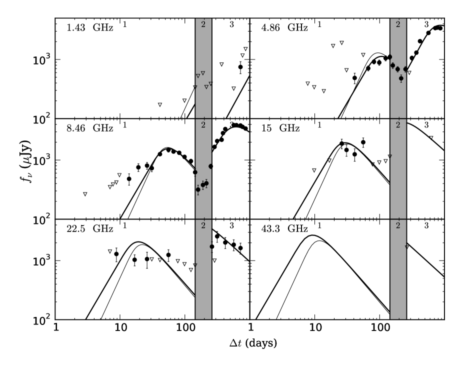
Figure 1: Light curves for SN 2007bg. Phase 1 is shown as the first white region, phase 2 is the shaded region and phase 3 the last white region. Different frequencies are represented by the following colours: $1.43$ GHz, $4.86$ GHz, $8.46$ GHz, $15$ GHz, $22.5$ GHz and $43.3$ GHz. We see a slow turn-on at $8.46$ GHz during phase 1. The lines during phase 1 represents the model fits. The thin line assumes a density profile $r\propto t^{0.94}$ and $B\propto t^{-1}$, while the thick line requires $r\propto t^{0.75}$ and $B\propto t^{-0.75}$. During this phase we modelled the emission as arising from a spherical expanding shell self that is absorbed by its own radiating electrons, as explained in §3.2. During phase 3 the line model represents our best fit model including the presence of SSA and a clumpy CSM. This is described in §3.4. Filled circles denote detections with $1\sigma$ error bars (which are smaller than symbols in some cases), while inverted triangles denote $3\sigma$ error limits.

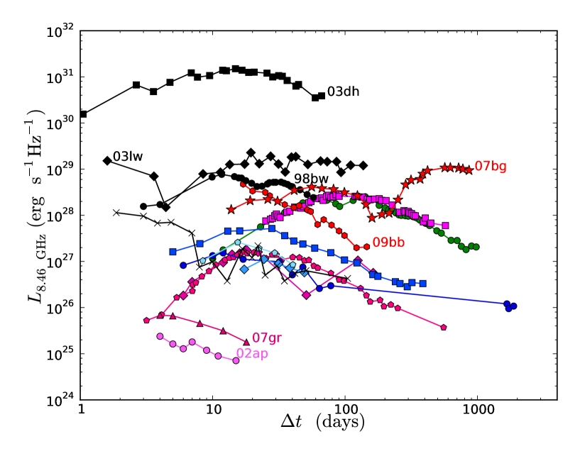
Figure 2: Radio light curves for different Type Ib SNe (shades of blue with different symbols) Type Ic’s (shades of pink with different symbols), a Type IIb SN (green) and GRBs (black with different symbols). SN 2007bg (red stars) is shown along with other objects. We observe that the radio luminosity from SN 2007bg is lower than that of GRBs on comparable time-scales and it is larger than in regular SNe at the time of the first peak during phase 1. Phase 3 starts at a comparable time-scale compared to other SNe, but the peak luminosity reached is larger by orders of magnitude. The SNe shown in this plot are Type Ic 2002ap (circles; Berger, Kulkarni & Chevalier, 2002), Type IIb 2003bg (circles; Soderberg et al., 2006a), Ic 2003L (squares; Soderberg et al., 2005), Ic 2004cc, Ib 2004dk, Ib 2004gq (diamonds; circles; squares; Wellons et al., 2012), Ic 1994I (pentagons; Weiler et al., 2011), Ic 2007gr (triangles; Soderberg et al., 2010a), Ib 2007uy, Ib/X-ray flash 2008D (diamonds; triangles; van der Horst et al., 2011) and Type Ic broad-lined 2009bb (hexagons; Soderberg et al., 2010b). Also, SNe associated with a GRBs Type Ic 1998bw (circles; Kulkarni et al., 1998), Ic 2003dh (squares; Hjorth et al., 2003; Kawabata et al., 2003; Matheson et al., 2003; Frail et al., 2005), Ic 2003lw (diamonds; Soderberg et al., 2004) and Ic 2006aj (Xs; Soderberg et al., 2006b).

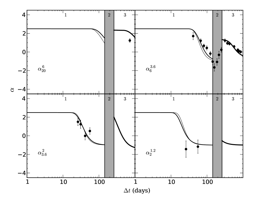
Figure 3: Spectral indices between adjacent bands. Over plotted are the predicted values from the light curve fitting as described in §3.2 and §3.4. The thin and thick lines represent the same models as in Fig. 1. Top left panel shows the evolution of the spectral index between $20$ cm and $6$ cm. Top right panel shows the spectral index from $6$ cm and $3.6$ cm, the best sampled set of observations. Bottom left spectral index between $3.6$ cm and $2$ cm. Bottom right spectral index between $2$ cm and $1.2$ cm. We note that near the end of phase 1 a large negative spectral index is observed, this is mainly because the light curve at $1.2$ cm deviates from the evolution observed at other wavelengths. Filled circles denote detections with $1\sigma$ error bars (which are smaller than symbols in some cases), while inverted triangles denote $3\sigma$ upper limits and triangles $3\sigma$ lower limits.

3 Results

The resulting light curves for SN 2007bg are shown in Fig. 1. The evolution of the light curves can be divided in three phases. Phase 1: this phase starts after the explosion and lasts until day $144$. Here we observe the typical turn-on of radio supernovae (RSNe), first starting at shorter wavelengths and cascading to longer wavelengths with time as wavelength-dependent absorption becomes less important. The peak luminosity reached during phase 1 is $4.1\times 10^{28}$ erg Hz^-1 s^-1 observed on day $55.9$ at $8.46$ GHz. This makes SN 2007bg one of the most luminous Type Ib/c RSNe on comparable time-scales. The first detections at $4.86$ and $8.46$ deviate from the rest of the evolution, and it could be due to interstellar scintillation, a real deviation from pure SSA due to clumpy CSM, or deceleration; unfortunately there is not enough early-time data to confirm it robustly. On day $55.9$ we also observe a rise in luminosity at $15$ and $22.5$ GHz, this could be the effect of a small density enhancement, since that would produce the achromatic variation observed, and as the lower frequencies are still optically thick it would not be noticed at these frequencies. Phase 2: if the shock is expanding into a constant (or even smoothly-varying) stellar wind, then after the absorption turn-on one expects the source to fade in intensity following a power-law decline with time. However on day $144$ the flux density consistently deviates from this at $8.46$ and $4.86$ GHz, showing a discontinuous drop in the observed flux density from days $\sim 144-250$. Phase 3: the luminosity of SN 2007bg begins a second turn-on around day $261.8$, becoming brighter than in phase 1 and reaching a peak luminosity of $1\times 10^{29}$ erg Hz^-1 s^-1 at $8.46$ GHz on day $566.9$. This late time behaviour is comparable to that of other Type Ib/c SNe like SN 2004cc, SN 2004dk and SN2004gq (Wellons, Soderberg & Chevalier, 2012), albeit much stronger and more well-defined than these other objects. There are also some Type IIb’s SNe which show late time modulations in their radio light curves. One of these is SN 2001ig (Ryder et al., 2004) in which case the late time modulations could be explained by a binary companion of the progenitor. Another example is SN 2003bg (Soderberg et al., 2006a), where the late time variations can not rule out a binary companion or different mass-loss episodes of the progenitor. In both cases the modulations in the light curve result from modulations in the CSM density. A comparison between SN 2007bg, other SNe and GRBs is shown in Fig. 2. During phase 1 the light curve of SN 2007bg resembles that of other SNe. It shows the characteristic turn-on, but with a higher luminosity than other normal Ib/c SNe and comparable to GRB-SNe. Then during phase 3 we observe a strong rise in its luminosity, which is unprecedented for SNe, as it reaches such high luminosities, $2.6$ times larger than during phase 1.

The spectral index, $f_{\nu}\propto\nu^{\alpha}$, evolution of the source is shown in Fig. 3. We observe a trend towards a negative value between the best sampled frequencies $4.86$ GHz and $8.46$ GHz during phase 1, but it could be that during this phase the source is still optically thick at $4.86$ GHz. If we assume that at this time the emission has reached its peak luminosity at $4.86$ GHz, then the late observed values of the spectral index point to a value of $\alpha\approx-1$. Even the deviant points at $15$ and $22.5$ GHz on day $55.9$ are consistent with this spectral index value. During phase 2 the source spectrum begins to invert. This behaviour continues during the first days of phase 3, indicating that some absorption mechanism becomes important again in phase 3. From the earliest spectral indices available we observe that the values are $\alpha\sim 2$, which is lower than the typical synchrotron self absorption (SSA) value of $2.5$ and the spectrum is shallower than the exponential cut-off expected from free-free absorption (FFA). This suggests may be observing a variety of emission regions from SN 2007bg; some being absorbed more highly than others. Since we can not resolve the source, we get the combined flux resulting in a shallower optically thick part of the spectrum.

Given that we do not have strong constraints on how the intrinsic spectral index varies with time, we adopt a fixed spectral slope for each phase of $\alpha\approx-1$.

3.1 Early Physical Constraints from Phase 1

Our first data point at $8.46$ GHz allows us to evaluate the brightness temperature of the source at $13.8$ days after explosion. The brightness temperature of the source should not exceed $3\times 10^{11}$ K if it is to remain under inverse Compton catastrophe (ICC), where the cooling time due to inverse Compton scattering is shorter than the synchrotron cooling time (Readhead, 1994) (see also; Kellermann & Pauliny-Toth, 1969). Using the measured flux density of $753$ $\mu$Jy at $8.46$ GHz, and if we assume that the optical expansion speed of $\sim 17500$ km s^-1, measured from the optical Ca II triplet, at $\sim 5$ days after explosion (Young et al., 2010) also pertains the radio emitting region, we obtain $T\approx 3.6\times 10^{12}$ K. This value is above the ICC limit, so one of our assumptions must be wrong. As discussed in the introduction, typically the radio ejecta from SNe have higher velocities than that of the photosphere, which produces the optical emission. Based on this we adopt a radius for the source such that the brightness temperature remains below the ICC limit constraining the source size to be $(7\pm 1)\times 10^{15}$ cm. The reported errors come from the flux density measurement uncertainty. At $13.8$ days after explosion this implies a bulk expansion speed of $\beta\Gamma\approx(0.2\pm 0.04)c$, where $\beta=v/c$ and $\Gamma$ is the Lorentz factor. This speed $v\approx(0.19\pm 0.03)c$ is $\approx 3$ times larger than that of the photosphere. We stress that this only a lower limit on the actual velocity at which the radio emitting region expands, as the radio ejecta could be expanding at a higher velocity and be well below the ICC brightness temperature. The resulting brightness temperature is shown in Fig. 4 where we assumed that the radio emitting region does not decelerate i.e., $r\propto t$.

Another way to estimate the expansion speed of the radio emitting region can be obtained by placing SN 2007bg in a luminosity peak time plot, which as discussed by Chevalier (1998) provides information about the average expansion speed of the radio emitting region. The plot is shown in Fig. 5 and we note that SN 2007bg has an average expansion speed of $\sim 0.2c$ typical of Type Ib/c RSNe and it shows one of the highest luminosities among Type Ib/c’s and comparable to those of GRBs. It is important to note that other absorption mechanisms, such as FFA, or deviations from equipartition, would increase the expansion velocity (and hence source energy, derived later).

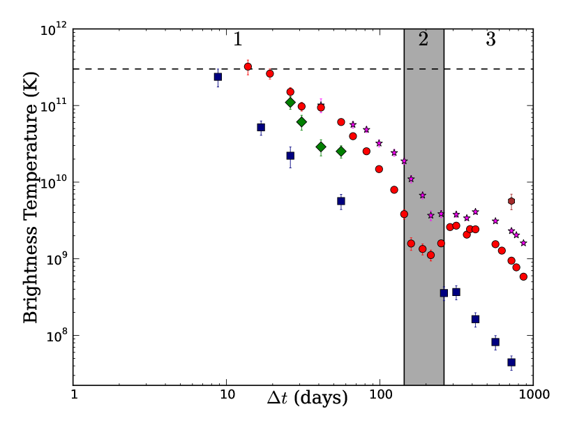
Figure 4: Brightness temperature curve for SN 2007bg using a constant bulk speed of $0.18c$. Different wavelengths are represented by different symbols, $1.43$ GHz (brown hexagons), $4.86$ GHz (magenta stars), $8.46$ GHz (red circles), $15$ GHz (green diamonds) and $22.5$ GHz (blue squares). The dashed line represents the ICC limit of $3\times 10^{11}$ K. The symbols are shown with their $1\sigma$ error bars (which are smaller than symbols in some cases). $3\sigma$ upper limits are represented by inverted triangles following the colour coding.

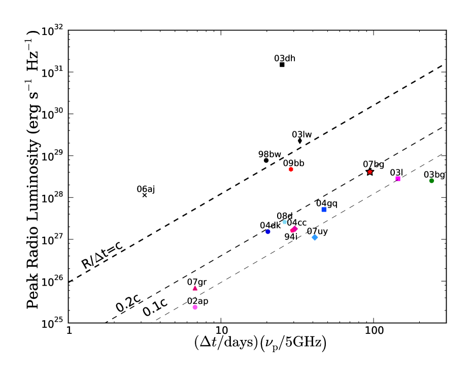
Figure 5: Source peak radio luminosity versus time of peak. The resulting position in this plot provides an estimate of the average expansion speed of the source. Some objects lie above $R/\Delta t=c$, because the emission from GRBs is different from that of SNe, for which this diagnostic was made. SN 2007bg lies at the high end of normal Type Ib/c SNe based on its high luminosity and shows an expansion speed of $\gamma\beta\approx 0.2c$. Here we have used data from phase 1 only. Other SNe and GRBs are the same as in Fig. 2. Error bars are small compared to the plot symbols.

3.2 Constraints from SSA Evolution during Phase 1

Synchrotron emission from SNe originates from the shock region between the SNe ejecta and the pre-existing CSM. This shock amplifies the existing magnetic fields via turbulence. The electrons in the shock region then interact with this magnetic field producing the observed synchrotron emission. This emission is subject to self-absorption, which is caused by SSA (Chevalier, 1998) in the case of low density environments. To describe the time evolution of the flux density during phase 1 we adopt the parametrization of Soderberg et al. (2005) in which the radio emission originates from a spherical thin shell of width $r/\eta$ expanding at a velocity $v$ in which the intrinsic synchrotron emission is absorbed by SSA. The parameter $\eta$ is the number of shells that fit into the size of the source with a value of $\eta\approx 10$ (Frail, Waxman & Kulkarni, 2000). We adopt the assumptions of the standard model of Chevalier (1982b) where the hydrodynamic evolution of the ejecta is self-similar across the shock discontinuity. With this assumption the radius of the source evolves as $r\propto t^{\alpha_{r}}$ where the parameter $\alpha_{r}$ is related to the density profile of the outer SN ejecta $\rho\propto r^{-n}$ and the density profile of the radiating electrons in the shock region $n_{\rm{e}}\propto r^{-s}$ such that $\alpha_{r}=(n-3)/(n-s)$. The self similar model also requires that $s<3$, $n>5$ and $\alpha_{r}$ in the range $0.75-1$. The model also assumes that the magnetic energy density and the relativistic electron energy density scale as the total post-shock energy density. This implies that the fraction of energy contained in the relativistic electrons $\epsilon_{\rm{e}}$ and magnetic field $\epsilon_{\rm{B}}$ remains fixed. This in turn relates the magnetic field evolution $B\propto t^{\alpha_{B}}$, to the radius of the source and the density profile of the radiating electrons $\alpha_{B}=(2-s)\alpha_{r}/2-1$. This means that for a freely expanding wind $s=2$, the magnetic field evolves as $B\propto t^{-1}$. For our analysis we adopt a source in equipartition with $\epsilon_{\rm{e}}=\epsilon_{\rm{B}}=0.1$. Equipartition of energy minimizes the total energy.

Using this model and requiring the time evolution of the magnetic field to go as $B\propto t^{-1}$ we find that the radius of the source evolves as $r\propto t^{0.94}$. We will refer to this as model 1. This is consistent with a shock expanding freely through the CSM. The normalization constants for the flux density and SSA are $C_{f}\approx 8.4\times 10^{-53}$ g s^-1 and $C_{\tau}\approx 8.5\times 10^{36}$ s^3.5, giving a reduced chi square value of $\chi_{r}=7.3$ for 22 degrees of freedom. These values require the size of the source to go as $r\approx 6.5\times 10^{15}(t/t_{0})^{0.94}$ cm, which in turn means that the expansion velocity is $v\approx 0.25(t/t_{0})^{-0.06}c$. The magnetic field goes as $B\approx 2.6(t/t_{0})^{-1}$ G and the energy is $E\approx 9.6\times 10^{47}$ erg. For this we assumed a synchrotron characteristic frequency of $\nu_{\rm{m}}=1$ GHz. Using these values we can also estimate the mass-loss rate of the progenitor. Following Soderberg et al. (2006a) we estimate a mass-loss rate of $\dot{M}\approx 1.5\times 10^{-6}(v_{w}/1000\;\rm{km\,s}^{-1})$ M${}_{\odot}\,$yr^-1. This mass-loss rate lies at the low end of those observed for WR stars in low metallicity environments (Crowther et al., 2002). The derived mass-loss rates from this model depend on the fraction of energy contained in relativistic electrons and magnetic fields, deviations from equipartition would require higher mass-loss rates and energy requirements.

The early data hint at a shallower slope of the light curve, so we also fit a second model, model 2, where we allow the magnetic field evolution to change as $B\propto t^{-0.75}$ and the source size as $r\propto t^{0.75}$. In this model the reduced chi square value is $\chi_{r}=4.4$ for 21 degrees of freedom. In this case the normalization constants are $C_{f}\approx 1.7\times 10^{-52}$ g s^-1 and $C_{\tau}\approx 4.6\times 10^{36}$ s^3.5. This implies a source size evolution of $r\approx 8.7\times 10^{15}(t/t_{0})^{0.74}$ cm, and an expansion velocity of $v\approx 0.3(t/t_{0})^{-0.25}c$. Given this expansion speed the source would remain below the ICC limit. The magnetic field goes as $B\approx 2.1(t/t_{0})^{-0.75}$ G. The source energy with these values is $E\approx 1.5\times 10^{48}$ erg, and the mass-loss rate is $\dot{M}\approx 1.9\times 10^{-6}(v_{w}/1000\;\rm{km\,s}^{-1})$ M${}_{\odot}\,$yr^-1. Here again we have used the same parameters for $\nu_{m}$ and $\eta$. Given this time evolution for the magnetic field and source size, the density radial profile goes as $\rho\propto r^{-8}$ and the number density of emitting electrons as $n_{\rm{e}}\propto r^{-1.3}$. We adopt the result from model 2, as it provides a better fit to the data, although we cannot truly rule out model 1 due to the lack of early detections.

Given this mass-loss rate, the circumstellar density for a wind stratified medium $A_{*}$, defined as $\dot{M}/4\pi v_{w}=5\times 10^{11}A_{*}$ g cm^-1 (Li & Chevalier, 1999), is $A_{*}\approx 0.2$. Under these conditions a relativistic jet from a GRB would become non-relativistic, and hence observable on a time-scale of $t_{\rm{NR}}\approx 0.3(E_{\rm{K}}/10^{51}\,\rm{erg})A_{*}^{-1}$. With the kinetic energy of the ejecta of $E_{\rm{K}}\approx 4\times 10^{51}$ erg, derived from the optical light curve (Young et al., 2010), this time-scale is $t_{\rm{NR}}\approx 6$ yr. The lack of clear afterglow signatures (e.g., Li & Chevalier, 1999; Waxman, 2004; Soderberg et al., 2006c) in our observations thus provide strong evidence against an expanding GRB jet being the source of the observed luminosity for SN 2007bg.

3.3 Stratified CSM: Phase 2

As can be seen in Fig. 1, at around day $144$ the flux density at $8.46$ and $4.86$ GHz suddenly decreases creating a break in the power law flux decay of the optically thin radio emission. At $8.46$ GHz the observed flux is a $44\%$ less than the predicted one at the beginning of phase 2 on day $159.8$. Based on the derived size of the radio emitting region, from the SSA modelling, this drop occurs at a distance of $\approx 6.7\times 10^{16}$ cm. The most likely cause for this decrease in the radio emission is a drop in the CSM density. Here we consider two scenarios that would produce a change in CSM density such as a binary companion or two different wind components from the progenitor star. In the first scenario, there should be evidence of this interaction from the optical spectra as Balmer series recombination lines. The late time optical spectra for SN 2007bg was too faint to be detected. The early optical spectra evidence points to a broad-lined SNe, most likely associated with SNe like 1998bw (Young et al., 2010), and the latest optical spectra of SN 2007bg where it is detected does not show evidence for a transition from a type Ib/c to a type II. For this kind of SNe the most likely progenitor is a single WR. Also if there was a binary companion we would expect to see coherence between the emission before and after the drop/increase (depending on whether the CSM density dropped/increased at the region of interest). In the case of SN 2007bg, we see a $>1$ dex jump in the normalizations of the unabsorbed phase 1 and phase 3 light curves, as well as a strong enhancement in absorption, making a binary companion CSM scenario highly unlikely. The second scenario considered is that the drop in flux density is due to a change in the progenitor wind. Based on the distance of the drop and with our assumed wind speed of $\approx 1000$ km s^-1 the change occurred $\approx 45$ yr before the explosion and lasted for $\approx 23$ yr. Since $L_{\nu}\propto(\dot{M}/v_{w})^{(\alpha-8+12\alpha_{r})/4}$ (Chevalier, 1982b) a flux density decrease of $44\%$ implies that the mass-loss rate/wind speed dropped by a factor of $\approx 5$. For this estimate we have used $\alpha_{r}=0.94$. Our modelling of the light curves during phase 1 suggests that the density profile of the CSM is shallower (i.e., smaller $\alpha_{r}$), but as discussed bellow, this relation overestimates the mass-loss rate in such cases.

3.4 Second Rise: Phase 3

Phase 3 begins around day $261.8$ with an increase in the flux density at $22.5$, $8.46$ and $4.86$ GHz. As discussed in §3 the luminosity of the source during this phase is larger than in phase 1 in all of the bands where we detect it. This flux density rise shows the characteristics of an absorption turn-on. At $22.5$ GHz we observe what appears to be the peak of the turn-on on day $314.8$, and at longer wavelengths the radio spectrum begins to turn-on near the end of observations. This turn-on is accompanied by an increase in the spectral index suggesting that the source has become optically thick again. The luminosity increase implies a sharp CSM density enhancement, presumably due to evolution of the progenitor wind, while the observed re-absorption requires either SSA or FFA. Following Fransson, Lundqvist & Chevalier (1996) we can estimate the mass-loss rate from the progenitor assuming that the absorption is purely FFA. Adopting the time of peak at $4.86$ GHz as the time when the free-free optical depth is unity, and taking the expansion velocity of the shock from phase 1 then the mass-loss rate is $\dot{M}\approx 10^{-1}(v_{w}/1000\;\rm{km\,s}^{-1})$ M${}_{\odot}\,$yr^-1. This rate is suspiciously high and inconsistent with our estimate (later in this section) of the mass-loss rate based on the unabsorbed portion of the spectrum. This high rate favours SSA. The absorption slope is relatively flat, and thus pure SSA with a similar model as fit to phase 1 does a poor job of fitting the turn-on. One possibility is differential SSA arising from small dense clumps in the CSM, which are preferentially affected by SSA while sparser regions are less affected; this naturally flattens the optically thick slope. The existence of clumpy winds in WR stars has been confirmed by observations (Moffat et al., 1988), and thus provides a natural way of explaining the observed radio emission. Alternatively, the density jump would naturally produce strong X-ray emission, which could ionize CSM material in front of the shock and provide the necessary free electrons for FFA. However, without constraints on the X-ray luminosity and phase 3 CSM density distribution for SN2007bg, it is difficult to assess the feasibility of FFA. Given the poor fit of the pure SSA model ($\chi_{r}=9$), we simply adopt the parametrization of Weiler et al. (2002) including only a clumpy CSM with the presence of internal SSA. In this case the flux density is normalised by $K_{1}$, the clumpy CSM absorption by $K_{3}$ and SSA by $K_{5}$. We fit the above model to the light curve during phase 3. The best-fit values are given in Table 4. The resulting reduced chi square of this fit is $\chi_{r}=4.4$ for 18 degrees of freedom.

Table 4: SN 2007bg best-fit values for phase 3.

Parameter	Adopted value
$\alpha$	$-1^{a}$
$\beta$	$-1^{b}$
$\alpha_{r}$	$1^{c}$
Parameter	Best-fit value
$K_{1}$	$5\times 10^{6}$
$K_{3}$	$2.3\times 10^{5}$
$\delta^{\prime}$	$-3.53$
$K_{5}$	$4.5\times 10^{8}$
$\delta^{\prime\prime}$	$-2.96$
a Adopted from observed values of $\alpha$.
b Assumed because of the lack of data.
c Computed using $\alpha_{r}=-(\alpha-\beta-3)/3$.

As shown in Fig. 1, this model provides a reasonable fit to the light curves at all frequencies and also to the spectral index, Fig. 3. The deviant point at $1.43$ GHz could be easily affected by the host galaxy luminosity. The data did not allow us to constrain the deceleration rate, so we adopted a constant expansion by fixing $\beta=-1$, which in turn requires that $\alpha_{r}=m=1$ given the spectral index. Using our best-fit values we can estimate the mass-loss rate from the progenitor during this period following equations (11) and (13) of Weiler et al. (2002). The effective optical depth at the time of our latest observation, $\sim 863$ days, at $4.86$ GHz is $\langle\tau_{\rm{eff}}^{0.5}\rangle\approx 2.2\times 10^{-3}$ and $m\approx 1$. If we extrapolate the velocity derived in §3.2 to phase 3, $v_{i}\approx 0.13c$ at $t_{i}\approx 300$ days, then the derived mass-loss rate is $\dot{M}\approx 4.3\times 10^{-4}(v_{w}/1000\;\rm{km\,s}^{-1})$ M${}_{\odot}\,$yr^-1, where an electron temperature of $10^{4}$ K was used. This mass-loss rate is higher than the one observed during phase 1, which is a natural explanation for the high luminosity observed during phase 3. However, such a large mass-loss rate has not yet been directly observed, and it is at odds with the metallicity mass-loss rate relation derived from the Milky Way and Magellanic Clouds WR samples (see for e.g., Crowther, 2006). This relation predicts orders of magnitude lower $\dot{M}$ in such a low metallicity host. On the other hand, this large mass-loss rate is also roughly consistent with that of the saturation limit for line-driven winds, $\dot{M}\approx 10^{-4}$ M${}_{\odot}\,$yr^-1, and is of the same order of magnitude as values found in other Type Ib/c SNe (e.g., Wellons et al., 2012). We should caution however that the dramatic flux increase between phases 1 and 3 implies a strong density contrast that is inconsistent with one of the primary assumptions of the Chevalier (1982b) self-similar model (namely a CSM density profile with a power-law slope). This density discontinuity could naturally lead to an overestimate of the mass-loss rate; to properly account for this type of case, one should generally model the hydrodynamics in detail; unfortunately, such simulations are not well-constrained by radio data alone due to ambiguities in how the B-field and electron density distribution might change across the density discontinuity and are beyond the scope of this work. Thus this phase 3 mass-loss rate should be regarded with caution and viewed as a likely upper limit. The strong mass-loss variations on such short time-scales seen here imply that the progenitor of SN 2007bg may have undergone unstable mass-loss just prior to explosion or a dramatic change in wind properties. Such rapid variations have been seen in a handful of objects before. For instance, in the case of Type Ib SN 2006jc (Pastorello et al., 2007), a bright optical transient was observed two years prior to explosion. This was interpreted as a luminous blue variable-like outburst event from the progenitor, which the later SN explosion surely interacted with. Then there are other possibilities like the case of Type IIn SN 1996cr (Bauer et al., 2008). In this event, the radio light curve also exhibits a strong late-time rise in emission associated with a density enhancement likely arising from the interaction of the SN blast-wave with a wind-blown bubble (Dwarkadas, Dewey & Bauer, 2010). The progenitor of SN 1996cr is proposed to be either a WR or blue supergiant star. We still know relatively little about why such global changes in the progenitors occur, but it seems clear that a subset of SNe progenitors have them.

3.5 X-Ray Constraints

X-ray emission from supernovae can arise from three mechanisms; non-thermal emission from synchrotron radiating electrons, thermal bremsstrahlung emission from the material in the circumstellar and reverse shocks, and inverse Compton emission. Since X-ray emission from SN 2007bg could not be detected it is difficult to assess the feasibility of each of these mechanisms, so we will compare the derived mass-loss rates from the previous subsections with that predicted by the thermal bremsstrahlung process.

If the X-ray emission comes from synchrotron radiating electrons then the X-ray luminosity can be obtained by extrapolating the radio synchrotron spectrum up to higher frequencies. To do this we must consider that the synchrotron spectrum changes its slope at the cooling frequency $\nu_{\rm{c}}\propto t^{-2}B^{-3}$ by a factor $\Delta\alpha\approx-0.5$ (Soderberg et al., 2005). Using the derived magnetic field $B$ from our SSA analysis of the radio light curve §3.2 we find that $\nu_{\rm{c}}\approx 323$ GHz. Extrapolation of the luminosity as $L_{\nu}\propto\nu^{-1.5}$ from the cooling break on gives a X-ray luminosity 5 orders of magnitude bellow our upper limit $\sim 30$ days after explosion (epoch 2). Extrapolation of the cooling frequency up to epochs 3 and 4 of the X-ray data yields X-ray fluxes $\sim 5$ orders of magnitude bellow the upper limits. However, as mentioned in previous sections, the CSM discontinuity between phases 1 and 3 could cause a break in the magnetic field evolution.

X-ray emission from thermal bremsstrahlung comes from the interaction of the shocked electrons with the circumstellar material. This interaction heats the electrons in the medium which then cool via free-free emission. In this process the X-ray luminosity is related to the density of the emitting material as $L\propto\dot{M}^{2}v_{w}^{-2}t^{-1}$ (Chevalier & Fransson, 2003; Sutaria et al., 2003). We can obtain an upper limit on the mass-loss rate from the X-ray luminosity upper limits using equation (30) of Chevalier & Fransson (2006). At $t\sim 30$ days the X-ray luminosity is $L_{0.5-8.0}<7.2\times 10^{39}$ erg s^-1. We use the density profile of the outer SNe ejecta derived from our SSA analysis, $\rho\propto r^{-8}$. Given this luminosity and CSM properties thermal bremsstrahlung requires a mass-loss rate of $\dot{M}<4.6\times 10^{-4}(v_{w}/1000\;\rm{km\,s}^{-1})$ M${}_{\odot}\,$yr^-1. At epochs 3 and 4 of the X-ray data we obtain mass-loss rates of $\dot{M}<3.6\times 10^{-3}(v_{w}/1000\;\rm{km\,s}^{-1})$ and $\dot{M}<1.4\times 10^{-2}(v_{w}/1000\;\rm{km\,s}^{-1})$ respectively. These mass-loss rates are consistent with the one required by SSA during phase 1 and the light curve during phase 3.

Inverse Compton scattering of the optical photons by the relativistic synchrotron emitting electrons can also be a cause of X-ray emission in SNe. It has been shown that this process played an important role in the case of SN 2002ap (Björnsson & Fransson, 2004), SN 2003L (Soderberg et al., 2005) and 2003bg (Soderberg et al., 2006a). Using equation (15) of Björnsson & Fransson (2004) we obtain a ratio of $U_{\rm{ph}}/U_{B}\sim 12$ $\sim 30$ days after explosion. For this we have used a bolometric luminosity of $L_{bol}\sim 10^{41.5}$ erg s^-1 based on the pseudo-bolometric light curves for SN 2007bg of Young et al. (2010). Given the ratio $U_{\rm{ph}}/U_{B}$ and the radio flux of $\nu F_{\nu}\approx 2\times 10^{-16}$ erg s^-1 cm^-2 the derived X-ray luminosity of $\sim 2\times 10^{-17}$ erg s^-1 cm^-2 is in agreement with our upper limits. For later epochs we can not estimate the bolometric luminosity of SN 2007bg.

4 Summary and Conclusions

In this article we presented the radio light curves and X-ray observations of Type Ic-BL SN 2007bg. The radio emission is characterised by three different phases. Phase 1 being characterised by a SSA turn-on. Based on the brightness temperature of SN 2007bg the expansion speed of the radio emitting region is $v=0.19\pm 0.02c$. An expansion speed similar to what has been found in the small sample of radio-emitting Type Ib/c SNe.

The derived mass-loss rate from the progenitor during phase 1 is $\dot{M}\approx 1.9\times 10^{-6}(v_{w}/1000\;\rm{km\,s}^{-1})$ M${}_{\odot}\,$yr^-1, a low mass-loss rate among the observed in WR stars. During phase 2 we observe a drop in the flux density while the spectral index seems to follow a smooth evolution. This drop is presumably due to the radio ejecta entering a region of lower CSM density, probably arising because of a change in the mass-loss rate of the progenitor or a variable wind speed. Then during phase 3 we observe a rise in the radio flux density along with a re-absorption of the radio emission. The shallow observed slope of the re-absorption could be explained by small clumps of material in the progenitor wind which would become more strongly self-absorbed than the surrounding CSM when shocked and produce a shallower optically-thick spectrum. From our modelling of the radio light curves during phase 3 we put an upper limit on the mass-loss rate of $\dot{M}\la 4.3\times 10^{-4}(v_{w}/1000\;\rm{km\,s}^{-1})$ M${}_{\odot}\,$yr^-1. This second wind component could arise from a different stellar evolution phase of the progenitor prior to explosion, possibly a LBV phase. Or it could be the effect of stellar rotation on the stellar wind properties. If the radio flux density from SN 2007bg declines in time like $f_{\nu}\propto t^{-1}$. It should still be detectable, with a flux density at $22.5$ GHz of $\sim 500$ $\mu$Jy, and higher at lower frequencies. If the progenitor star went through more mass-loss episodes, then the observed flux density would deviate from this value. Recent observations taken with the Karl G. Jansky Very Large Array (JVLA) should help to establish this. Very few broad-lined type Ic SNe have radio detections, and none of them show signs of a complex CSM like that of SN 2007bg.

These different wind components, along with the derived mass-loss rates will eventually help to constrain the progenitors of Type Ib/c SNe, from their inferred pre-SNe properties. Currently two main evolutionary paths has been proposed to account for the rate of these explosions: a single WR origin, and a binary system. However, the single WR scenario itself still needs significant clarification. For instance, what effects do evolution (mass-loss, rotation, etc.) and metallicity have in shaping the CSM around massive type Ib/c progenitors and ultimately their explosions. And more generally, how does this fold into the connection between type II’s, type Ib/c, and GRBs.

Compounded by their relative rarity, a key impediment to improving our knowledge of broad-lined Ic SNe has been the lack of high-quality, multi-frequency observations from early through late epochs. Sensitive high-frequency radio observations of Ic SNe within 1-2 days of explosion are needed to efficiently identify the best objects for follow-up and allow further refinement of the physical properties surrounding these unique explosions. Both ALMA and the newly retooled JVLA will play critical roles here, providing rigorous probes of the synchrotron-emitting shock (to constrain evolution of the shock velocity, any potential beaming, etc.) and ultimately new insights into the properties of their CSM (such as density, variability, clumpiness, and perhaps even dust content for these massive systems). Sensitive, long-term X-ray and optical/NIR spectroscopic follow-up are also needed in order to break potential degeneracies and provide consistency checks against the shock-CSM interaction models. If such complete datasets can be assembled in the next several years, they may afford us a leap in our physical understanding of SNe and GRBs.

References

- Bauer et al. (2008) Bauer F. E., Dwarkadas V. V., Brandt W. N., Immler S., Smartt S., Bartel N., Bietenholz M. F., 2008, ApJ, 688, 1210
- Berger et al. (2002) Berger E., Kulkarni S. R., Chevalier R. A., 2002, ApJL, 577, L5
- Björnsson & Fransson (2004) Björnsson C.-I., Fransson C., 2004, ApJ, 605, 823
- Bufano et al. (2012) Bufano F., et al., 2012, ApJ, 753, 67
- Chevalier (1982a) Chevalier R. A., 1982a, ApJ, 258, 790
- Chevalier (1982b) Chevalier R. A., 1982b, ApJ, 259, 302
- Chevalier (1998) Chevalier R. A., 1998, ApJ, 499, 810
- Chevalier & Fransson (2003) Chevalier R. A., Fransson C., 2003, in Weiler K., ed., Supernovae and Gamma-Ray Bursters Vol. 598 of Lecture Notes in Physics, Berlin Springer Verlag, Supernova Interaction with a Circumstellar Medium. pp 171–194
- Chevalier & Fransson (2006) Chevalier R. A., Fransson C., 2006, ApJ, 651, 381
- Crowther (2006) Crowther P. A., 2006, in Lamers H. J. G. L. M., Langer N., Nugis T., Annuk K., eds, Stellar Evolution at Low Metallicity: Mass Loss, Explosions, Cosmology Vol. 353 of Astronomical Society of the Pacific Conference Series, Observed Metallicity Dependence of Winds from WR stars. p. 157
- Crowther et al. (2002) Crowther P. A., Dessart L., Hillier D. J., Abbott J. B., Fullerton A. W., 2002, A&A, 392, 653
- Dickey & Lockman (1990) Dickey J. M., Lockman F. J., 1990, ARA&A, 28, 215
- Dwarkadas et al. (2010) Dwarkadas V. V., Dewey D., Bauer F., 2010, MNRAS, 407, 812
- Frail et al. (2005) Frail D. A., Soderberg A. M., Kulkarni S. R., Berger E., Yost S., Fox D. W., Harrison F. A., 2005, ApJ, 619, 994
- Frail et al. (2000) Frail D. A., Waxman E., Kulkarni S. R., 2000, ApJ, 537, 191
- Fransson et al. (1996) Fransson C., Lundqvist P., Chevalier R. A., 1996, ApJ, 461, 993
- Galama et al. (1998) Galama T. J., et al., 1998, Nature, 395, 670
- Hjorth & Bloom (2011) Hjorth J., Bloom J. S., 2011, arXiv:1104.2274
- Hjorth et al. (2003) Hjorth J., et al., 2003, Nature, 423, 847
- Humphreys & Davidson (1994) Humphreys R. M., Davidson K., 1994, PASP, 106, 1025
- Kawabata et al. (2003) Kawabata K. S., et al., 2003, ApJL, 593, L19
- Kellermann & Pauliny-Toth (1969) Kellermann K. I., Pauliny-Toth I. I. K., 1969, ApJL, 155, L71
- Kraft et al. (1991) Kraft R. P., Burrows D. N., Nousek J. A., 1991, ApJ, 374, 344
- Kulkarni et al. (1998) Kulkarni S. R., et al., 1998, Nature, 395, 663
- Li & Chevalier (1999) Li Z.-Y., Chevalier R. A., 1999, ApJ, 526, 716
- Matheson et al. (2003) Matheson T., et al., 2003, ApJ, 599, 394
- Modjaz et al. (2006) Modjaz M., et al., 2006, ApJL, 645, L21
- Moffat et al. (1988) Moffat A. F. J., Drissen L., Lamontagne R., Robert C., 1988, ApJ, 334, 1038
- Paragi et al. (2010) Paragi Z., et al., 2010, Nature, 463, 516
- Pastorello et al. (2007) Pastorello A., et al., 2007, Nature, 447, 829
- Podsiadlowski et al. (1992) Podsiadlowski P., Joss P. C., Hsu J. J. L., 1992, ApJ, 391, 246
- Prieto et al. (2008) Prieto J. L., Stanek K. Z., Beacom J. F., 2008, ApJ, 673, 999
- Prieto et al. (2009) Prieto J. L., Watson L. C., Stanek K. Z., 2009, The Astronomer’s Telegram, 2065, 1
- Quimby et al. (2007) Quimby R., Rykoff E., Yuan F., 2007, Central Bureau Electronic Telegrams, 927, 1
- Readhead (1994) Readhead A. C. S., 1994, ApJ, 426, 51
- Ryder et al. (2004) Ryder S. D., Sadler E. M., Subrahmanyan R., Weiler K. W., Panagia N., Stockdale C., 2004, MNRAS, 349, 1093
- Smartt (2009) Smartt S. J., 2009, ARA&A, 47, 63
- Smith et al. (2011) Smith N., Li W., Filippenko A. V., Chornock R., 2011, MNRAS, 412, 1522
- Soderberg (2009) Soderberg A. M., 2009, The Astronomer’s Telegram, 2066, 1
- Soderberg et al. (2010a) Soderberg A. M., Brunthaler A., Nakar E., Chevalier R. A., Bietenholz M. F., 2010a, ApJ, 725, 922
- Soderberg et al. (2006a) Soderberg A. M., Chevalier R. A., Kulkarni S. R., Frail D. A., 2006a, ApJ, 651, 1005
- Soderberg et al. (2004) Soderberg A. M., et al., 2004, Nature, 430, 648
- Soderberg et al. (2006b) Soderberg A. M., et al., 2006b, Nature, 442, 1014
- Soderberg et al. (2010b) Soderberg A. M., et al., 2010b, Nature, 463, 513
- Soderberg et al. (2005) Soderberg A. M., Kulkarni S. R., Berger E., Chevalier R. A., Frail D. A., Fox D. B., Walker R. C., 2005, ApJ, 621, 908
- Soderberg et al. (2006c) Soderberg A. M., Nakar E., Berger E., Kulkarni S. R., 2006c, ApJ, 638, 930
- Stanek et al. (2003) Stanek K. Z., et al., 2003, ApJL, 591, L17
- Sutaria et al. (2003) Sutaria F. K., Chandra P., Bhatnagar S., Ray A., 2003, A&A, 397, 1011
- van der Horst et al. (2011) van der Horst A. J., et al., 2011, ApJ, 726, 99
- Van Dyk et al. (2003) Van Dyk S. D., Li W., Filippenko A. V., 2003, PASP, 115, 1
- Vink et al. (2000) Vink J. S., de Koter A., Lamers H. J. G. L. M., 2000, A&A, 362, 295
- Waxman (2004) Waxman E., 2004, ApJ, 602, 886
- Weiler et al. (2002) Weiler K. W., Panagia N., Montes M. J., Sramek R. A., 2002, ARA&A, 40, 387
- Weiler et al. (2011) Weiler K. W., Panagia N., Stockdale C., Rupen M., Sramek R. A., Williams C. L., 2011, ApJ, 740, 79
- Wellons et al. (2012) Wellons S., Soderberg A. M., Chevalier R. A., 2012, ApJ, 752, 17
- Woosley & Bloom (2006) Woosley S. E., Bloom J. S., 2006, ARA&A, 44, 507
- Woosley & Weaver (1986) Woosley S. E., Weaver T. A., 1986, ARA&A, 24, 205
- Xu et al. (2011) Xu M., Nagataki S., Huang Y. F., 2011, ApJ, 735, 3
- Young et al. (2010) Young D. R., et al., 2010, A&A, 512, A70