Synthetic Aperture Radar Imaging and Motion Estimation
via Robust Principal Component Analysis

Abstract

We consider the problem of synthetic aperture radar (SAR) imaging and motion estimation of complex scenes. By complex we mean scenes with multiple targets, stationary and in motion. We use the usual setup with one moving antenna emitting and receiving signals. We address two challenges: (1) the detection of moving targets in the complex scene and (2) the separation of the echoes from the stationary targets and those from the moving targets. Such separation allows high resolution imaging of the stationary scene and motion estimation with the echoes from the moving targets alone. We show that the robust principal component analysis (PCA) method which decomposes a matrix in two parts, one low rank and one sparse, can be used for motion detection and data separation. The matrix that is decomposed is the pulse and range compressed SAR data indexed by two discrete time variables: the slow time, which parametrizes the location of the antenna, and the fast time, which parametrizes the echoes received between successive emissions from the antenna. We present an analysis of the rank of the data matrix to motivate the use of the robust PCA method. We also show with numerical simulations that successful data separation with robust PCA requires proper data windowing. Results of motion estimation and imaging with the separated data are presented, as well.

1 Introduction

In synthetic aperture radar (SAR), the basic problem [6, 16, 7] is to image the reflectivity supported in a set ${\cal J}^{{}^{\cal I}}$ on the ground surface using measurements obtained with an antenna system mounted on a platform flying above it, as illustrated in Figure 1. The antenna emits periodically a probing signal $f(t)$ and records the echos $D(s,t)$, indexed by the slow time $s$ of the SAR platform displacement and the fast time $t$. The slow time parametrizes the location $\vec{\bf r}(s)$ of the platform at the instant it emits the signal, and the fast time $t$ parametrizes the echoes received between two consecutive illuminations $\left(0<t<\Delta s\right)$.

Figure 1: Setup for synthetic aperture imaging.

The echoes $D(s,t)$ are approximately, and up to a multiplicative factor, a superposition of the emitted signals $f(t)$ time-delayed by the round-trip travel-time between the platform $\vec{\bf r}(s)$ and the locations $\vec{\boldsymbol{\rho}}$ of scatterers on the ground

$$\tau\left(s,\vec{\boldsymbol{\rho}}\right)=2\left|\vec{\bf r}(s)-\vec{\boldsymbol{\rho}}\right|/c.$$ (1.1)

Here $c$ is the wave speed, assumed constant and equal to the speed of light.

A SAR image is formed by superposing over a platform trajectory of length (aperture) $a$ the data $D(s,t)$ convolved with the time reversed emitted signal (matched filtered), and then backpropagated to points in the imaging domain ${\cal J}^{{}^{\cal I}}$ using travel times. With high bandwidth probing signals and large flight apertures, SAR is capable of generating images with roughly ten centimeter resolution at ranges of ten kilometers away from the platform. Such resolution cannot be achieved for complex scenes because moving targets appear blurred and displaced in the images. Image formation should therefore be done in conjunction with target motion estimation. In fact, in applications such as persistent surveillance SAR, tracking and imaging the moving targets is one of the primary objectives.

Because targets may have complicated motion over lengthy data acquisition trajectories, the targets are tracked over successive small sub-apertures. Each sub-aperture corresponds to a short time interval over which the target is in approximate uniform translational motion. The problem is to estimate this motion for each time interval in order to bring the small aperture images of the moving targets into focus. Then, the images are superposed to form high resolution images over larger apertures.

The existing algorithms for motion estimation fall roughly into two categories: The first is for the usual SAR setup with a single moving antenna, and the target motion is estimated from the phase modulations of the return echoes [2, 9, 8, 1, 21, 24, 13, 15, 18, 20, 10]. These algorithms assume that all the targets are in the same motion, and are sensitive to the presence of strong stationary targets. The second class of methods uses more complex antenna systems [14, 23, 22], with multiple receiver and/or transmitter antennas. They form a collection of images with the echoes measured by each receiver-transmitter pair, and then they use the phase variation of the images with respect to the receiver/transmitter offsets, pixel by pixel, to extract the target velocity.

In this paper we consider imaging and motion estimation of complex scenes with the usual SAR setup, using a single antenna. We address two challenges: (1) the detection of moving targets in the scene and (2) the separation of data in subsets of echoes from the stationary scene and echoes from the moving targets. The stationary scene can be imaged by itself after such separation, and the motion estimation can be carried out on the echoes from the moving targets alone. We propose and analyze a detection and data separation approach based on the robust principle component analysis (robust PCA) method [4]. Robust PCA is designed to decompose a matrix into a low rank one plus a sparse one. The main contribution of this paper is to show with analysis and numerical simulations that by appropriately pre-processing and windowing the SAR data we can decompose it into a low rank part, corresponding to the stationary scene, and a sparse part, corresponding to the moving targets. Our theoretical and numerical study describes the rank of the pre-processed SAR data as a function of the velocity, location, and density of the scatterers. It specifies in particular how slowly a target can move and still be distinguishable from the stationary scene. It also addresses the question of proper windowing of the data for the separation with robust PCA to work.

The paper is organized as follows: We begin in section 2 with a brief description of basic SAR data processing and image formation. There are two processing steps that are key to the data decomposition: pulse compression and range compression. We illustrate with numerical simulations in section 3 that robust PCA can be used for motion detection and data separation if it is complemented with proper data windowing. The analysis is in section 4. Additional numerical results on data separation, motion estimation and imaging are in section 5. We end with a summary in section 6.

2 Basic SAR data processing and image formation

The antenna emits signals that consist of a base-band waveform $f_{B}(t)$ modulated by a carrier frequency $\nu_{o}=\omega_{o}/(2\pi)$,

$$f(t)=\cos(\omega_{o}t)f_{B}(t).$$ (2.2)

Its Fourier transform is

$$\widehat{f}(\omega)=\int dt\,f(t)e^{i\omega t}=\frac{1}{2}\left[\widehat{f}_{B}(\omega+\omega_{o})+\widehat{f}_{B}(\omega-\omega_{o})\right],$$ (2.3)

with $\widehat{f}_{B}(\omega)$ supported in the interval $[-\pi B,\pi B]$, where $B$ is the bandwidth. The support of $\widehat{f}(\omega)$ is the same interval with center shifted at $\omega_{o}$, and its mirror image in the negative frequencies.

Imaging relies on accurate estimation of travel times. Recall that the echoes are approximately, up to some amplitude factors, superpositions of the emitted signals delayed by the round trip travel times between the antenna and the targets in the scene. Suppose that

$$f_{B}(t)=\varphi(Bt),$$

with $\varphi$ a function of a dimensionless argument and compact support in the unit interval $[0,1]$. Then $f_{B}(t)$ has the form of a pulse, and the travel times can be estimated with precision $1/B$, the pulse support. But such pulses are almost never used in SAR because of power limitations at the antenna [16]. The SAR echoes should be above the antenna’s noise level, so the emitted signals should carry large power. However, the instantaneous power at the antenna is limited, while large net power can be delivered by longer signals, such as chirps. The problem is that the received scattered energy is spread out over the long time support of such signals, making it impossible to resolve the time of arrival of different echoes. This is overcome by compressing the long echoes, as if they were created by an incident pulse. This pulse compression amounts to convolving the data with the complex conjugate of the time reversed emitted signal $f(-t)$

$$D_{p}(s,t)=\int dt^{\prime}\,D(s,t^{\prime})\overline{f\left(t^{\prime}-t\right)}.$$ (2.4)

The result is as if the antenna emitted the signal

$$f_{p}(t)=\int dt^{\prime}\,f(t^{\prime})\overline{f\left(t^{\prime}-t\right)},$$

which turns out to be a pulse of support $1/B$, as explained in detail in [16].

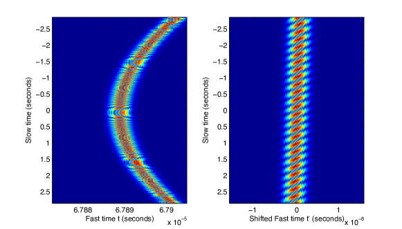
Figure 2: Left: Pulse compressed data $D_{p}(s,t)=f(t-\tau(s,\vec{\boldsymbol{\rho}}))$ from a single scatterer at $\vec{\boldsymbol{\rho}}=(0,5,0)$, recorded by a SAR antenna moving at speed $V=70$ m/s along a linear aperture of $400$ m, at range $L=10$ km from $\vec{\boldsymbol{\rho}}$. Note the hyperbolic curve defined by the peak. Right: Pulse and range-compressed data $D_{r}(s,t^{\prime})$ with respect to point $\vec{\boldsymbol{\rho}}_{o}=(0,0,0)$. The abscissa is the shifted fast time $t^{\prime}$. Note that most of the slow time dependence is removed in the range-compressed data.

Another common data pre-processing step is range compression. It amounts to evaluating the pulse compressed data at times offset by the round trip travel time to a reference point $\vec{\boldsymbol{\rho}}_{o}\in{\cal J}^{{}^{\cal I}}$,

$$D_{r}(s,t^{\prime})=D_{p}(s,t^{\prime}+\tau(s,\vec{\boldsymbol{\rho}}_{o})).$$ (2.5)

Here $t^{\prime}$ is the fast time shifted by $\tau(s,\vec{\boldsymbol{\rho}}_{o})$, so that

$$t^{\prime}+\tau(s,\vec{\boldsymbol{\rho}}_{o})=t\in[0,\Delta s].$$

In the Fourier domain, the range compression amounts to removing the large phase $\omega\tau(s,\vec{\boldsymbol{\rho}}_{o})$ of $\widehat{D}_{p}(s,\omega)$. This is obviously advantageous from the computational point of view. But range compression plays a bigger role in our context. It is essential for the robust PCA method to work. To illustrate this, we show in Figure 2 the pulse compressed echo from a single scatterer, for a linear aperture. The scatterer is at $\vec{\boldsymbol{\rho}}=(0,5,0)$, with the first two coordinates defining the location in the imaging plane and the third the elevation, which is always zero. The coordinates in the imaging plane are range and cross-range, with origin at the reference point. The range is the coordinate of $\vec{\boldsymbol{\rho}}$ along the direction pointing from the SAR platform (at the center of the aperture) to $\vec{\boldsymbol{\rho}}_{o}$. The cross-range is the coordinate of $\vec{\boldsymbol{\rho}}$ in the direction orthogonal to the range.

We plot in Figure 2 the amplitude of $D_{p}(s,t)$ as a function of $s$ and $t$, and note that the location of the peak, defined by equation

$$\left(\frac{ct}{2}\right)^{2}=|\vec{\bf r}(s)-\vec{\boldsymbol{\rho}}|^{2},$$

is a hyperbola for the linear aperture. The peak lies on some other curve in the $(s,t)$ plane for other apertures. The amplitude of the range compressed data is shown in the right plot of Figure 2. We note that the dependence on the slow time $s$ has been approximately removed by the range compression. Explicitly, it lies on the curve in the $(s,t^{\prime})$ plane defined by equation

$$\frac{ct^{\prime}}{2}=|\vec{\bf r}(s)-\vec{\boldsymbol{\rho}}|-|\vec{\bf r}(s)-\vec{\boldsymbol{\rho}}_{o}|.$$

This curve is close to the vertical axis $t^{\prime}=0$ because $\vec{\boldsymbol{\rho}}$ and $\vec{\boldsymbol{\rho}}_{o}$ are close to each other,

$$|\vec{\boldsymbol{\rho}}-\vec{\boldsymbol{\rho}}_{o}|\ll|\vec{\bf r}(s)-\vec{\boldsymbol{\rho}}|,\qquad\forall s.$$

Consequently, the matrix with entries $D_{r}(s,t)$, sampled at discrete $s$ and $t$, appears to be of low rank and it can be handled by the robust PCA method.

We work with the pulse and range compressed data from now on, and to simplify notation, we drop the prime from the shifted fast time $t^{\prime}$. We borrow terminology from the geophysics literature and call the pulse and range compressed echoes data traces. The image is formed by superposing the traces over the aperture, and backpropagating them to the imaging points $\vec{\boldsymbol{\rho}}^{\,\cal I}\in{\cal J}^{{}^{\cal I}}$ using travel times

$${\cal I}\left(\vec{\boldsymbol{\rho}}^{{\cal I}}\right) = \sum_{j=-n/2}^{n/2}D_{r}(s_{j},\tau(s_{j},\vec{\boldsymbol{\rho}}^{\,\cal I})-\tau(s_{j},\vec{\boldsymbol{\rho}}_{o}))$$ (2.6)

$$\approx \frac{1}{\Delta s}\int_{-S(a)}^{S(a)}ds\,D_{r}(s,\tau(s,\vec{\boldsymbol{\rho}}^{\,\cal I})-\tau(s,\vec{\boldsymbol{\rho}}_{o})).$$

Here $s_{j}$ are the discrete slow time samples in the interval $[-S(a),S(a)]$ defining the aperture $a$ along the flight track. The sampling is uniform, at intervals $\Delta s$, and

$$2S(a)=n\Delta s,\quad\mbox{with}~{}n~{}\mbox{even}.$$

Assuming a large $n$, that is a small $\Delta s$, we approximate the sum in (2.6) by an integral over the aperture.

When the aperture is very large, the data in (2.6) is weighted by a factor that compensates for geometrical spreading effects over the long flight track, and thus improves the focus of the image. Here we work with small apertures where geometrical spreading plays no role, which is why there are no weights in the imaging function (2.6).

3 Robust PCA for motion detection and SAR data separation

We begin in section 3.1 with a brief discussion of the robust PCA method. Then, we give in section 3.2 a heuristic explanation of why it makes sense to use it for motion detection and data separation. We also illustrate in section 3.3 the difficulties arising in the separation, and the improvements achieved by proper data windowing.

3.1 Robust PCA

The robust PCA method, introduced and analyzed in [4], applies to matrices $M\in\mathbb{R}^{n_{1}\times n_{2}}$ that are sums of a low rank matrix ${\cal L}_{o}$ and a sparse matrix ${\cal S}_{o}$. It solves a convex optimization problem called principle component pursuit:

$$\min_{{\cal L},{\cal S}\in\mathbb{R}^{n_{1}\times n_{2}}}\quad||{\cal L}||_{*}+\eta||{\cal S}||_{1}$$ (3.1)

$$\text{subject to}\quad{\cal L}+{\cal S}=M,$$ (3.2)

with

$$\eta=\frac{1}{\sqrt{\max\{n_{1},n_{2}\}}}.$$ (3.3)

Here $||{\cal L}||_{*}$ is the nuclear norm, i.e. the sum of the singular values of ${\cal L}$, and $||{\cal S}||_{1}$ is the matrix 1-norm of ${\cal S}$. The optimization can be done for any matrix, but the point is that if $M={\cal L}_{o}+{\cal S}_{o}$, with ${\cal L}_{o}$ low rank and $S_{o}$ sparse and high rank, then the principle component pursuit recovers exactly ${\cal L}_{o}$ and ${\cal S}_{o}$. The analysis in [4] gives sufficient conditions under which the decomposition is exact. These conditions are bounds on the rank of ${\cal L}_{o}$ and the number of non-zero entries in the high rank matrix ${\cal S}_{o}$. They are not necessary conditions, meaning that the decomposition can be achieved for a much larger class of matrices than those fulfilling the assumptions of the theorems in [4]. This is already pointed out in [4].

3.2 The structure of the matrix of range compressed SAR data

We illustrate in this section the pulse and range compressed echoes (the traces) from a complex scene. The point of the illustration is to show that typically, the sampled traces from the stationary scene form a low rank matrix, whereas those from moving targets give a high rank but sparse matrix. We refer to section 5 for the description of the setup of the numerical simulations used to produce the results presented here and in the next section.

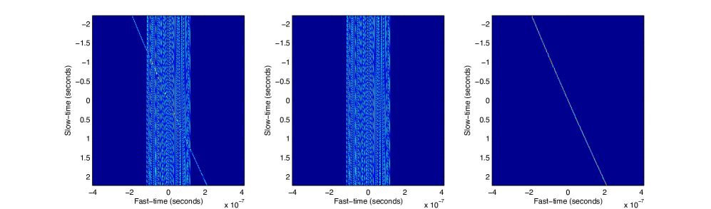
Figure 3: Desired separation of the range and pulse compressed SAR data. Left: $|D_{r}(s,t)|$ for a sample scene with thirty stationary targets. The vertical traces correspond to the stationary targets, while the sloped trace corresponds to the moving target. Middle: The stationary component of $|D_{r}(s,t)|$. Right: The moving component of $|D_{r}(s,t)|$. We plot the absolute value of these matrices only to increase contrast for the figures.

Let $M$ be the matrix with entries given by the data traces sampled at the discrete slow and fast times

$$M_{jl}=D_{r}(s_{j},t_{l}),$$ (3.4)

where

$$s_{j}=j\Delta s,\quad j=-n/2,\ldots,n/2,$$ (3.5)

and

$$t_{l}=l\Delta t,\quad l=-m/2,\ldots,m/2.$$ (3.6)

The sampling is at uniform intervals $\Delta s$ and $\Delta t$, and $n$ and $m$ are positive integers satisfying

$$2S=n\Delta s,\quad\mbox{and}\quad\Delta s=m\Delta t.$$ (3.7)

We assume throughout that $n$ and $m$ are even and large.

We show in the left plot of Figure 3 the matrix $M$ for a scene with a single moving target and thirty stationary scatterers. The ideal separation of this matrix would be

$$M={\cal L}_{o}+{\cal S}_{o}$$

where ${\cal L}_{o}$ is given by the echoes from the stationary targets alone and ${\cal S}_{o}$ is given by the echo from the moving target. We plot ${\cal L}_{o}$ and ${\cal S}_{o}$ in the middle and right plot of Figure 3. It appears to the eye that ${\cal L}_{o}$ is a matrix with almost parallel columns, so we expect it to be low rank. The matrix ${\cal S}_{o}$ is given by the sloped curve in the $(s,t)$ plane. The range compression does not remove the $s$ dependence of the echo from the moving target, as is the case for the stationary ones, and this is why we see this sloped curve. Consequently, ${\cal S}_{o}$ has higher rank than ${\cal L}_{o}$. But it is sparse, because we have only one moving target, i.e., one sloped curve. Obviously, the matrix ${\cal S}_{o}$ will remain sparse for a small number of moving targets, as well.

Thus, the matrix $M$ appears to have the appropriate structure for the robust PCA method to be useful. But we show next that robust PCA alone will not do the job adequately. It must be complemented with proper data windowing.

3.3 Data windowing for separation with robust PCA

We illustrate with two numerical simulations that robust PCA cannot be applied as a black box to the SAR data traces and produce the desired separation of the stationary and moving target parts. However, if it is applied to properly calibrated subsets (or windows) of the data, robust PCA can separate the traces for a large class of complex scenes.

The results of the first simulation are in Figure 4. We have a scene with seven stationary targets at coordinates $(0,0,0)$m, $(\pm 5,0,0)$m, $(0,\pm 5,0)$m and $(\pm 10,0,0)$m in the imaging plane, which is at elevation zero. There is also a moving target that is at location $(0,0,0)$, at slow time $s=0$ corresponding to the center of the aperture. The target moves with velocity ${\bf u}=\frac{28}{\sqrt{2}}(1,1)$m/s in the plane. We refer to section 5 for a detailed description of the setup for the simulations. In the top row of plots in Figure 4 we show the results with robust PCA applied to the matrix $M$ of data traces shown on the left. The middle and right plots are the resulting low rank and sparse parts given by the robust PCA algorithm. Due to the fact that the entire matrix $M$ is sparse to begin with, much of the stationary target data is captured by the sparse component. Thus, we do not have a good separation. However, the result is very good when we apply the robust PCA algorithm on a smaller fast-time window of the data, as shown in the second row of plots. The number of nonzero entries in the windowed $M$ is no longer small relative to its size, and robust PCA separates the moving target trace from the rest.

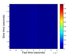
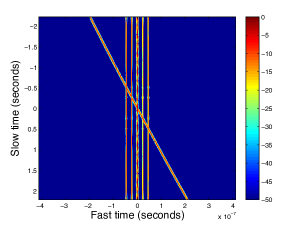
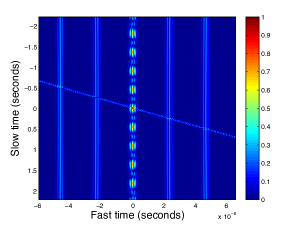
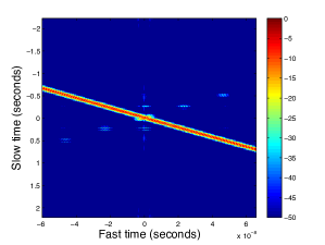
Figure 4: Robust PCA separation of traces from a scene with seven stationary targets and a moving target. From left to right we show the matrix $M$ of traces, the low rank ${\cal L}$, and sparse ${\cal S}$ components from robust PCA. Top row is robust PCA applied to the entire data, bottom row is robust PCA applied to a windowed part of the data. In each plot the matrices are normalized by the largest value of $|D_{r}(s,t)|$. The sparse components shown in the right column are plotted in (decibel) dB scale to make the contrast more visible.

In Figure 6 we show the results for a scene with thirty stationary targets and a moving one. The data traces from this scene are displayed in Figure 5. The moving target is as in the previous example. The point of the simulation is to show that when we work in a large fast time window the traces from all the stationary targets may no longer form a low rank matrix. The top row of plots in Figure 6 shows that the sparse component of the matrix $M$, as returned by the robust PCA algorithm, has a large residual part from the stationary targets. The much improved results in the bottom are obtained by applying robust PCA on successive small fast time windows of the data, and then reassembling the separated traces. To give an idea of the size of the windows, the matrix $M$ has dimensions $n=296$ by $m=16,384$. The matrices are windowed in fast-time and are of size $296\times 450$.

Figure 5: SAR scene with thirty stationary targets and a moving one.

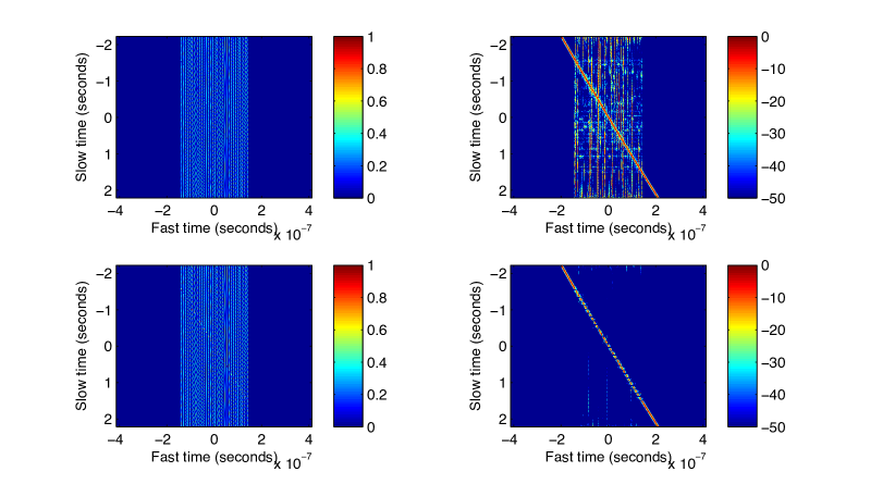
Figure 6: Robust PCA separation of traces from a scene with thirty stationary targets and a moving one. The top row of plots shows the results with robust PCA applied to the entire data matrix in Figure 5. The low rank and sparse components are shown in the middle and on the right. The bottom row of plots shows the results with robust PCA applied to successive small time windows of the data. The sparse components shown in the right column are plotted in dB scale to make the contrast more visible.

The two examples given above show that data windowing plays an important role in achieving a successful data separation with robust PCA. The last simulation also illustrates the role of robust PCA in the detection of the moving target. While the trace from this target is faint and difficult to distinguish from the others over most of the fast time interval in Figure 5, it is clearly visible in Figure 6 after the processing of the traces with robust PCA.

4 Analysis of rank of the matrix of SAR data traces

We present here an analysis of the rank of the matrix of SAR data traces for simple scenes with one or two targets. The goal is to understand how the rank depends on the position of the targets and their velocity. We limit the analysis to at most two targets to get a simple structure of the matrix $MM^{T}$, for which we can calculate the rank almost explicitly. The numerical results presented above and in section 5 show that the data separation works for complex scenes, with many stationary targets.

We begin in section 4.1 with the scaling regime used in the analysis. We illustrate it with the GOTCHA Volumetric SAR data set [5] for X-band surveillance SAR. The model of the matrix $M$ is given in section 4.2. We analyze its rank in section 4.3 for a single target, and in section 4.4 for two targets. We end with a brief discussion in section 4.5.

4.1 Scaling regime and illustration with GOTCHA volumetric SAR

The important scales in the problem are: The central frequency $\nu_{o}$, the bandwidth $B$, the typical distance (range) $L$ from the SAR platform to the targets, the aperture $a$, the magnitude $|{\bf u}|$ of the speed of the targets, the speed $V$ of the SAR platform and $R^{{\cal I}}$, the diameter of the imaging set ${\cal J}^{{}^{\cal I}}$. We assume that they are ordered as follows

$$B\ll\nu_{o},$$ (4.1)

and

$$a\ll L,\quad R^{{}^{\cal I}}\ll L,$$ (4.2)

and we let

$$L=|\vec{\bf r}(0)-\vec{\boldsymbol{\rho}}_{o}|.$$ (4.3)

We also suppose that the target speed is smaller than that of the SAR platform

$$|{\bf u}|<V.$$ (4.4)

As an illustration, consider the setup in GOTCHA Volumetric SAR. The central frequency of the probing signal is $\nu_{0}=9.6$GHz and the bandwidth is $B=622$MHz, so assumption (4.1) holds. The SAR platform trajectory is circular, at height $H=7.3$km, with radius $R=7.1$km and speed $V=250$km/h or $70$m/s. One circular degree of trajectory is $124$m. The pulse repetition rate is $117$ per degree, which means that a pulse is sent every $1.05$m, and $\Delta s=0.015$s. A typical distance to a target is $L=10$km and we consider imaging domains of radius $R^{{}^{\cal I}}$ of at most $50$m, so assumptions (4.2) hold. The target speed is $|{\bf u}|\sim 100$km/h or $28$m/s, so it satisfies (4.4).

For a stationary target we obtain from basic resolution theory (for single small aperture imaging) that the range can be estimated with precision $c/B=48$cm, and the cross range resolution is $\lambda_{0}L/a=2.5$m, with one degree aperture $a$ and central wavelength $\lambda_{0}=3$cm. The image of a moving target is out of focus unless we estimate its velocity and compensate for the motion in the imaging function.

4.2 Data model

Our model of the data assumes that the scatterers lying on the imaging surface behave like point targets. We neglect any interaction between the scatterers, meaning that we make the single scattering, Born approximation. The pulse and range compressed data is approximated by

$$D_{r}(s,t)\approx\sum_{q=1}^{N}\frac{\sigma_{q}(\omega_{o})}{(4\pi|\vec{\bf r}(s)-\vec{\boldsymbol{\rho}}_{q}(s)|)^{2}}f_{p}(t-(\tau(s,\vec{\boldsymbol{\rho}}_{q}(s))-\tau(s,\vec{\boldsymbol{\rho}}_{o}))),$$ (4.5)

in the case of $N$ targets at locations

$$\vec{\boldsymbol{\rho}}_{q}(s)=(\boldsymbol{\rho}_{q}(s),0),\quad q=1,\ldots,N,$$

with reflectivity $\sigma_{q}(\omega_{o})$. Here we used the so-called stop-start approximation which neglects the displacement of the targets during the round trip travel time. This is justified in radar because the waves travel at the speed of light that is many orders of magnitude larger than the speed of the targets. We refer to [2] for a derivation of the model (4.5) in the scaling regime described above.

Because of our scaling assumptions (4.2), we can approximate the amplitude factors as

$$\frac{1}{4\pi|\vec{\bf r}(s)-\vec{\boldsymbol{\rho}}_{q}(s)|}\approx\frac{1}{4\pi L},$$

and obtain the simpler model

$$D_{r}(s,t)=\left(\frac{1}{4\pi L}\right)^{2}\sum_{q=1}^{N}\sigma_{q}f_{p}(t-\Delta\tau(s,\vec{\boldsymbol{\rho}}_{q}(s))),$$ (4.6)

where we let

$$\Delta\tau(s,\vec{\boldsymbol{\rho}}(s))=\tau(s,\vec{\boldsymbol{\rho}}(s))-\tau(s,\vec{\boldsymbol{\rho}}_{0}).$$ (4.7)

We assume henceforth, for simplicity, that the targets are identical

$$\sigma_{q}=\sigma,\quad q=1,\ldots,N,$$

and write

$$D_{r}(s,t)\approx\frac{\sigma(\omega_{o})}{(4\pi L)^{2}}{\mathcal{M}}(s,t),$$ (4.8)

with

$${\mathcal{M}}(s,t)=\sum_{q=1}^{N}f_{p}(t-\Delta\tau(s,\vec{\boldsymbol{\rho}}_{q}(s))).$$ (4.9)

The matrix of traces analyzed below is given by discrete samples of (4.9),

$$M_{jl}={\mathcal{M}}\left(s_{j-\frac{n}{2}-1},t_{l-1}\right),\quad j=1,\ldots,n+1,~{}~{}l=1,\ldots,m+1,$$ (4.10)

with slow times $s_{j}$ and fast times $t_{l}$ defined in (3.5) and (3.6). We also take for convenience a compressed pulse given by a Gaussian modulated by a cosine at the central frequency,

$$f_{p}(t)=\cos(\omega_{o}t)e^{-B^{2}t^{2}/2}.$$ (4.11)

4.3 Analysis of rank of the data traces for one target

In the case of one target at location $\vec{\boldsymbol{\rho}}(s)=(\boldsymbol{\rho}(s),0)$, the entries of matrix (4.10) are given by

$$M_{jl}=\cos\left[\omega_{o}(t-\Delta\tau(s,\vec{\boldsymbol{\rho}}(s)))\right]\exp\left[-\frac{B^{2}}{2}(t-\Delta\tau(s,\vec{\boldsymbol{\rho}}(s)))^{2}\right],$$ (4.12)

with $\Delta\tau$ defined by (4.7). The target is moving at speed $\vec{\bf u}=({\bf u},0)$, so we have that

$$\vec{\boldsymbol{\rho}}(s)=\vec{\boldsymbol{\rho}}+s\,\vec{{\bf u}},\quad|s|\leq S(a),$$ (4.13)

where we let

$$\vec{\boldsymbol{\rho}}:=\vec{\boldsymbol{\rho}}(0)$$

be the location of the target at the time $s=0$, corresponding to the center of the aperture.

We study the rank of $M$, which is equivalent to studying the rank of the symmetric, square matrix $C\in\mathbb{R}^{(n+1)\times(n+1)}$, with entries given by

$$C_{j,l}={\cal C}\left(s_{j-\frac{n}{2}-1},s_{l-\frac{n}{2}-1}\right),\qquad j,l=1,\ldots,n+1,$$ (4.14)

in terms of the function

$${\cal C}(s,s^{\prime})=\sum_{q=-m/2}^{m/2}D_{r}(s,t_{q})D_{r}(s^{\prime},t_{q})\approx\frac{1}{\Delta t}\int_{-\infty}^{\infty}dt\ D_{r}(s,t)D_{r}(s,t).$$ (4.15)

Here we used the assumption that $\Delta t$ is small enough to approximate the Riemann sum over $q$ by the integral over $t$. Because the traces $D_{r}(s,t)$ vanish for $|t|>\Delta s/2$, we extended the integral to the whole real line.

We obtain after a calculation given in appendix A that if the aperture $a$ is small enough, the matrix $C$ has a Toeplitz structure.

Proposition 1

Assuming that the Fresnel number $\frac{a^{2}}{\lambda_{o}L}$ is bounded by

$$\frac{a^{2}}{\lambda_{o}L}\ll\min\left\{\frac{L}{R^{{}^{\cal I}}},\frac{V}{|\vec{\bf u}|}\right\},$$ (4.16)

the matrix $C$ is approximately Toeplitz, with entries given by

$${\cal C}(s,s^{\prime})\approx\frac{\sqrt{\pi}}{2B\Delta t}\cos\left[\omega_{o}\alpha(s-s^{\prime})\right]\exp\left[-\frac{(B\alpha)^{2}(s-s^{\prime})^{2}}{4}\right].$$ (4.17)

The dimensionless parameter $\alpha$ depends linearly on the velocity in the range direction and the cross-range offset of the target with respect to the reference point $\vec{\boldsymbol{\rho}}_{o}$. It is given by

$$\alpha=\frac{2\vec{\bf u}\cdot\vec{{\bf m}}_{o}}{c}-\frac{2V\vec{{\bf t}}\cdot\mathbb{P}_{o}(\vec{\boldsymbol{\rho}}-\vec{\boldsymbol{\rho}}_{o})}{cL}+\frac{2\vec{\bf u}\cdot\mathbb{P}_{o}(\vec{\boldsymbol{\rho}}-\vec{\boldsymbol{\rho}}_{o})}{cL},$$ (4.18)

with $\vec{{\bf m}}_{o}$ the unit vector pointing in the range direction from the center $\vec{\bf r}(0)$ of the aperture

$$\vec{{\bf m}}_{o}=\frac{\vec{\bf r}(0)-\vec{\boldsymbol{\rho}}_{o}}{|\vec{\bf r}(0)-\vec{\boldsymbol{\rho}}_{o}|},$$ (4.19)

and $\mathbb{P}_{o}$ the orthogonal projection

$$\mathbb{P}_{o}=I-\vec{{\bf m}}_{o}\vec{{\bf m}}_{o}^{T}.$$ (4.20)

The unit vector $\vec{{\bf t}}$ is defined by

$$\frac{d\vec{\bf r}(0)}{ds}=V\vec{{\bf t}}.$$ (4.21)

It is tangential to the flight track, at the center of the aperture.

Figure 7: The matrix $C$ for one stationary target at $\vec{\boldsymbol{\rho}}=(0,15,0)$m. The reference point is $\vec{\boldsymbol{\rho}}_{o}=\vec{\bf 0}$. The aperture is $310$m, the range $L=10$km and the central wavelength is $\lambda_{o}=3$cm. The plot shows that the matrix is essentially constant along the diagonals, it is approximately Toeplitz.

As an illustration, we plot in Figure 7 the matrix $C$ for an aperture $a=310$m, in the GOTCHA regime with central wavelength $\lambda_{o}=3$cm and range $L=10$km. We have a stationary target at $\vec{\boldsymbol{\rho}}=(0,15,0)$m, and $\vec{\boldsymbol{\rho}}_{o}$ is at the origin. The Fresnel number

$$\frac{a^{2}}{\lambda_{o}L}=320.3$$ (4.22)

is only half the ratio $L/R^{{}^{\cal I}}$, with $R^{{}^{I}}=15$m, and yet the matrix $C$ is essentially Toeplitz.

Remark: Since

$$\|D_{r}(s,\cdot)\|^{2}_{2}=\frac{\sqrt{\pi}}{2B\Delta t},\quad\forall s,$$

the angle between two rows of the matrix $M$ of data traces, indexed by $s$ and $s^{\prime}$, is given by

$$\cos\angle(D_{r}(s\cdot),D_{r}(s^{\prime},\cdot))\approx\cos[\omega_{o}\alpha(s-s^{\prime})]\exp\left[-\frac{(B\alpha)^{2}(s-s^{\prime})^{2}}{4}\right].$$ (4.23)

Nearby rows with indices satisfying

$$\alpha|s-s^{\prime}|<\frac{1}{B},$$

are nearly parallel, with a small, rapidly fluctuating angle between them. But rows that are far apart, with indices satisfying

$$\alpha|s-s^{\prime}|\geq\frac{3\sqrt{2}}{B},$$

are essentially orthogonal, because the right hand side in (4.23) is approximately zero. When the target is stationary, and its cross-range offset is zero, then $\alpha=0$, and all the entries in $C$ are constant and equal to one. Moreover, all the rows of $M$ are parallel to each other, and the matrix has rank one. When we view the data traces we see a vertical line at $t=0$, as in the left plot of Figure 8. Obviously, the larger $|\alpha|$ is, the closer the indices of the rows that are nearly orthogonal. So we expect the rank of $M$ to increase with $|\alpha|$. This is indeed the case, as we show next. We also illustrate this fact in the right plot of Figure 8, where we show the matrix of data traces for a stationary target that is offset from the reference point $\vec{\boldsymbol{\rho}}_{o}$. Note that by definition (4.18), $|\alpha|$ is large when the cross-range offset of the target and/or the target speed are large.

Figure 8: Matrix $M$ of data traces for a stationary target located at $\vec{\boldsymbol{\rho}}=\vec{\boldsymbol{\rho}}_{o}=(0,0,0)$m (left) and at $\vec{\boldsymbol{\rho}}=(-10,-10,0)$m (right).

4.3.1 Asymptotic characterization of the rank

Because matrix $C$ is Toeplitz and large, we can use the asymptotic Szegő theory [17, 3] to estimate its rank. To do so, let us define the sequence $\{c_{j}\}_{j\in\mathbb{Z}}$ with entries

$$c_{j}=\frac{\sqrt{\pi}}{2B\Delta t}e^{-\frac{(\xi j)^{2}}{4}}\cos(\xi j),\qquad\xi=B|\alpha|\Delta s.$$ (4.24)

A finite set of this sequence, for indices $|j|\leq n$, defines approximately the diagonals of the matrix $C$,

$$C_{j,l}\approx c_{j-l},\quad j,l=1,\ldots,n+1.$$ (4.25)

Since multiplication of a large Toeplitz matrix with a vector is approximately a convolution, and since convolutions are diagonalized by the Fourier transform, it is not surprising that the spectrum of $C$ is defined in terms of the symbol $Q(\theta)$, the coefficients of the Fourier series of (4.24),

$$Q(\theta)=\sum_{j=-\infty}^{\infty}c_{j}e^{ij\theta},\quad\quad\theta\in(-\pi,\pi).$$ (4.26)

With this symbol, we can characterize asymptotically in the limit $n\to\infty$ the rank of $C$, using Szegő’s first limit theorem [3], that gives

$$\lim_{n\to\infty}\frac{{\cal N}(n;\beta_{1},\beta_{2})}{n+1}=\frac{1}{2\pi}\int_{-\pi}^{\pi}1_{[\beta_{1},\beta_{2}]}(Q(\theta))d\theta.$$ (4.27)

Here $1_{[\beta_{1},\beta_{2}]}$ is the indicator function of the interval $[\beta_{1},\beta_{2}]$ and ${\cal N}(n;\beta_{1},\beta_{2})$ is the number of eigenvalues of $C$ that lie in this interval.

We show in appendix B that the symbol is given approximately by

$$Q(\theta)\approx\frac{\pi}{2B\Delta t\xi}\left\{\exp\left[-\frac{(\theta-\gamma)^{2}}{\xi^{2}}\right]+\exp\left[-\frac{(\theta+\gamma)^{2}}{\xi^{2}}\right]\right\},$$ (4.28)

where $\gamma\in(-\pi,\pi)$ is defined by

$$\gamma=[(\omega_{0}\alpha\Delta s+\pi)\mod 2\pi]-\pi.$$ (4.29)

We use this result and (4.27) to obtain an asymptotic estimate of the essential rank, defined by

$$\mbox{rank}\left[C\right]:={\cal N}\left(n;\epsilon\|Q\|_{\infty},\infty\right),\quad\quad\|Q\|_{\infty}=\sup_{\theta\in(-\pi,\pi)}|Q(\theta)|.$$ (4.30)

Here $0<\epsilon\ll 1$ is a small threshold parameter, and $\|Q\|_{\infty}$ is of the order of the largest singular value of $C$. It follows from the Szegő theory [17, 3] that this singular value is given by the maximum of the symbol, which is of the order of $\pi/(2B\Delta t\xi)$. We obtain that for $n\gg 1$,

$$\frac{\mbox{rank}\left[C\right]}{n+1} \approx \frac{1}{2\pi}\int_{-\pi}^{\pi}1_{[\epsilon\|Q\|_{\infty},\infty)}(Q(\theta))d\theta$$ (4.31)

$$= \min\left(\frac{2|\alpha|B\Delta s\sqrt{\log 1/\epsilon}}{\pi},1\right),$$

where the last equality follows from direct calculation.

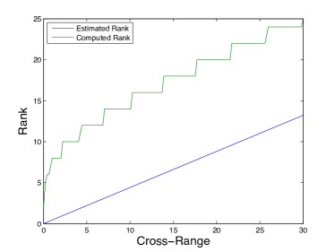
(a) Stationary

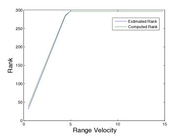
(b) Moving

Figure 9: Comparison of the computed and estimated rank of $C$ for a single target. Left: Stationary target at various cross-range positions. Right: Moving target with various velocities.

As an illustration, we show with green in Figure 9a the computed rank of the matrix $C$ for a single stationary target, versus the cross-range position. Positions with larger cross-range result in larger $|\alpha|$ and thus larger rank, as expected. The asymptotic estimate (4.31) of the rank is shown in blue. It exhibits the same linear growth in cross-range and therefore in $|\alpha|$, but it is lower than the computed rank. This is because in this simulation $n$ is not sufficiently large. We get a good approximation when $c_{j}\approx 0$ for $j\approx n$, so we can approximate the series (4.26) that defines the symbol by the truncated sum for indices $|j|\leq n$. This is not the case in this simulation, so there is a discrepancy in the estimated rank. However, the result improves when we increase $n$, by increasing the aperture. This is illustrated in Figure 10, where we show the rank normalized by the size of the matrix, and note that it has the predicted asymptote as $n$ increases.

The plot in Figure 9b shows the computed rank (in green) and the asymptotic estimate (4.31) (in blue) for a moving target located at $\vec{\boldsymbol{\rho}}=\vec{\boldsymbol{\rho}}_{o}$ at $s=0$. We plot the rank as a function of the range component of the velocity. The rank increases with the velocity, and therefore with $|\alpha|$, as expected. Moreover, the asymptotic estimate is very close to the computed one, because in this case the entries in the sequence $\{c_{j}\}_{j\in\mathbb{Z}}$ decay faster with $j$. Finally, notice that even for small velocities, the rank is much larger for the moving target than the stationary target.

Figure 10: Convergence of the rank of $C$ normalized by the size $(n+1)$. The blue line is the computed value and the green line is the asymptotic estimate.

4.4 Analysis of the rank of the data traces for two targets

In the case of two targets at locations $\vec{\boldsymbol{\rho}}_{j}(s)$ for $j=1,2$, the entries of the matrix $M$ follow from equations (4.9) and (4.10),

$$M_{jl}=\sum_{j=1}^{2}\cos\left[\omega_{o}(t-\Delta\tau(s,\vec{\boldsymbol{\rho}}_{j}(s)))\right]\exp\left[-\frac{B^{2}}{2}(t-\Delta\tau(s,\vec{\boldsymbol{\rho}}_{j}(s)))^{2}\right].$$ (4.32)

We take for simplicity the case of two stationary targets

$$\vec{\boldsymbol{\rho}}_{j}(s)=\vec{\boldsymbol{\rho}}_{j}:=\vec{\boldsymbol{\rho}}_{j}(0),\quad j=1,2.$$

Extensions to moving targets with speeds $\vec{\bf u}_{1}$ and $\vec{\bf u}_{2}$ are straightforward. They amount to redefining the parameters $\alpha_{1}$ and $\alpha_{2}$ defined below by adding two linear terms in the target velocity, as in equation (4.18).

The expression of matrix $C=MM^{T}$ is given in the following proposition. It is obtained with a calculation that is similar to that in appendix A, using the same assumption on the Fresnel number as in Proposition 1.

Proposition 2

Assume that the Fresnel number satisfies the bound (4.16), with $\vec{\bf u}=0$ since the targets are stationary. The matrix $C$ has entries defined by the function

$${\cal C}(s,s^{\prime}) \approx\frac{\sqrt{\pi}}{2B\Delta t}\left\{\sum_{j=1}^{2}\cos[\omega_{o}\alpha_{j}(s-s^{\prime})]\exp\left[-\frac{(B\alpha_{j})^{2}(s-s^{\prime})^{2}}{4}\right]\right.$$

$$+\cos[\omega_{o}(\alpha_{1}s-\alpha_{2}s^{\prime}+\beta)]\exp\left[-\frac{B^{2}(\alpha_{1}s-\alpha_{2}s^{\prime}+\beta)^{2}}{4}\right]$$ (4.33)

$$\left.+\cos[\omega_{o}(\alpha_{1}s^{\prime}-\alpha_{2}s+\beta)]\exp\left[-\frac{B^{2}(\alpha_{1}s^{\prime}-\alpha_{2}s+\beta)^{2}}{4}\right]\right\},$$

sampled at the discrete slow times. Here we let

$$\alpha_{j}=-\frac{2V\vec{{\bf t}}\cdot\mathbb{P}_{o}(\vec{\boldsymbol{\rho}}_{j}-\vec{\boldsymbol{\rho}}_{o})}{cL},$$ (4.34)

and

$$\beta=\frac{2}{c}\sum_{j=1}^{2}(-1)^{j}\left\{\vec{{\bf m}}_{o}\cdot(\vec{\boldsymbol{\rho}}_{j}-\vec{\boldsymbol{\rho}}_{o})+\frac{[\vec{{\bf m}}_{o}\cdot(\vec{\boldsymbol{\rho}}_{j}-\vec{\boldsymbol{\rho}}_{o})]^{2}}{2L}\right\}.$$ (4.35)

The structure of the matrix $C$ is now more complicated. The first term in (4.33) gives a Toeplitz matrix, as before. The other two, which are due to the interaction between the targets, give matrices that are approximately g-Toeplitz or g-Hankel, depending on the sign of the ratio $\alpha_{2}/\alpha_{1}$.

Definition 1

An $(n+1)\times(n+1)$ g-Hankel matrix $H$ with shift $g\in\mathbb{Z}^{+}$ is defined by a sequence $\{h_{j}\}_{j\in\mathbb{N}}$ as

$$H_{jl}=h_{j-1+g(l-1)},\qquad j,l=1,\ldots,n+1.$$

The matrix is Hankel when $g=1$. A g-Toeplitz matrix is defined similarly, by replacing $g$ with $-g$.

To analyze the spectrum of matrix $C$, we choose the reference point $\vec{\boldsymbol{\rho}}_{o}$ in such a way that

$$\frac{\alpha_{2}}{\alpha_{1}}<0,\quad\mbox{and}\quad g:=\left|\frac{\alpha_{2}}{\alpha_{1}}\right|\in\mathbb{N}.$$ (4.36)

Then, $C$ is given by

$$C=T+H+H^{T},$$ (4.37)

with Toeplitz matrix

$$T_{jl}=c_{j-l},\qquad j,l=1,\ldots,n+1,$$ (4.38)

and g-Hankel matrix

$$H_{jl}=h_{(j-1)+g(l-1)},\qquad j,l=1,\ldots,n+1.$$ (4.39)

Here $\{c_{j}\}_{j\in\mathbb{Z}}$ and $\{h_{j}\}_{j\in\mathbb{N}}$ are sequences with entries

$$c_{j}=\frac{\sqrt{\pi}}{2B\Delta t}\left[e^{-\frac{(\xi_{1}j)^{2}}{4}}\cos(\xi_{1}j)+e^{-\frac{(\xi_{2}j)^{2}}{4}}\cos(\xi_{2}j)\right],\quad\xi_{\ell}=B|\alpha_{\ell}|\Delta s,\quad\ell=1,2$$ (4.40)

and

$$h_{j}=\frac{\sqrt{\pi}}{2B\Delta t}e^{-\frac{[\xi_{1}(j+\zeta)]^{2}}{4}}\cos[\xi_{1}(j+\zeta)],\qquad\zeta=\frac{\beta}{|\alpha_{1}|\Delta s}.$$ (4.41)

An example of matrix $C$ and its Toeplitz and g-Hankel parts is shown in Figure 11.

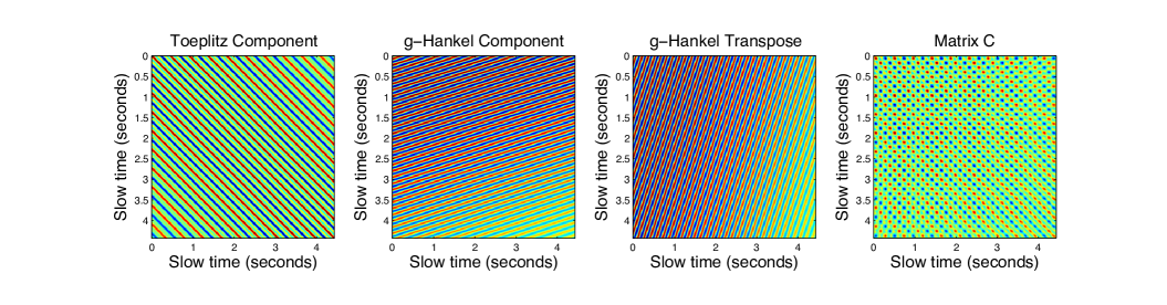
Figure 11: Components of matrix $C$ for two stationary targets located at $\vec{\boldsymbol{\rho}}_{1}=(0.15,15,0)$m and $\vec{\boldsymbol{\rho}}_{2}=(-0.15,-5,0)$m. On the left we show the Toeplitz part $T$. The next two plots show the g-Hankel part $H$ and its transpose $H^{T}$. The right plot shows the sum, i.e., the matrix $C$.

If the range offsets are large, so that

$$\xi_{1}|\zeta|=B|\beta|=\frac{2B}{c}\left|\sum_{j=1}^{2}(-1)^{j}\{\vec{{\bf m}}_{o}\cdot(\vec{\boldsymbol{\rho}}_{j}-\vec{\boldsymbol{\rho}}_{o})+\frac{[\vec{{\bf m}}_{o}\cdot(\vec{\boldsymbol{\rho}}_{j}-\vec{\boldsymbol{\rho}}_{o})]^{2}}{2L}\right|\gg 1,$$

the g-Hankel matrix has small entries, and $C$ is approximately Toeplitz, as in the single target case. The difference of the travel times between the SAR platform and such targets is larger than the compressed pulse width, and their interaction in (4.33) is negligible. If the range offsets are small, the structure of the matrix $C$ is as in equation (4.37), and the estimate of its rank follows from the recent results in [19, 11, 12]. They say that the g-Hankel terms $H+H^{T}$ have a negligible effect on the rank in the limit $n\to\infty$. See appendix C for more details. Thus, in either case, the rank estimate of $C$ is given by equation (4.27), in terms of the symbol $Q(\theta)$ defined by (4.26), using the sequence $\{c_{j}\}_{j\in\mathbb{Z}}$ with entries (4.40).

Explicitly, the symbol is given by

$$Q(\theta)\approx\frac{\pi}{2B\Delta t\xi_{1}}\left[e^{-\frac{(\theta-\gamma_{1})^{2}}{\xi_{1}^{2}}}+e^{-\frac{(\theta+\gamma_{1})^{2}}{\xi_{1}^{2}}}\right]+\frac{\pi}{2B\Delta t\xi_{2}}\left[e^{-\frac{(\theta-\gamma_{2})^{2}}{\xi_{2}^{2}}}+e^{-\frac{(\theta+\gamma_{2})^{2}}{\xi_{2}^{2}}}\right],$$ (4.42)

with $\gamma_{j}\in(-\pi,\pi)$ defined by

$$\gamma_{j}=[(\omega_{0}\alpha_{j}\Delta s+\pi)\mod 2\pi]-\pi,$$ (4.43)

for $j=1,2$, and the rank is given by

$$\mbox{rank}\left[C\right]\approx\frac{(n+1)}{2\pi}\int_{-\pi}^{\pi}1_{[\epsilon\|Q\|_{\infty},\infty)}(Q(\theta))d\theta.$$ (4.44)

Figure 12: Data traces from two stationary targets. Left: the targets are at positions $\vec{\boldsymbol{\rho}}_{1}=(2,5,0)$m and $\vec{\boldsymbol{\rho}}_{2}=(-2,15,0)$m. Middle: $\vec{\boldsymbol{\rho}}_{1}=(2,5,0)$m and $\vec{\boldsymbol{\rho}}_{2}=(-2,5,0)$m. Right: $\vec{\boldsymbol{\rho}}_{1}=(0.15,5,0)$m and $\vec{\boldsymbol{\rho}}_{2}=(-0.15,15,0)$m.

4.4.1 Illustration

We compare in Figure 13 the computed and estimated rank for two stationary targets. The results on the left are for one target fixed at location $\vec{\boldsymbol{\rho}}_{1}=(5,5,0)$m. We vary the location of the other target between $(-5,0.01,0)$m and $(-5,30,0)$m. The range separation is $10$m, so that $B|\beta|=41.47,$ and the g-Hankel matrix $H$ has negligible entries. The results on the right are for one target at $\vec{\boldsymbol{\rho}}_{1}=(0.15,5,0)$m and the location of the other varying between $(-0.15,0.01,0)$m to $(-0.15,30,0)$m. The range separation is $0.3$m, so that $B|\beta|=1.24,$ and the g-Hankel matrix $H$ is no longer negligible. We see that in spite of $H$ being neglible or not, the rank of matrix $C$ behaves essentially the same, as predicted by the asymptotic theory. This would be difficult to guess by just looking at the data traces displayed in Figure 12.

The computed and the estimated ranks grow at the same rate with the cross range of the second target, i.e., with $|\alpha_{2}|$. The growth is monotone except in the vicinity of the local minimum corresponding to the targets having exactly the same cross-range. In this special configuration $\alpha_{1}=\alpha_{2}$, and therefore $\xi_{1}=\xi_{2}$. The symbol (4.42) simplifies to

$$Q(\theta)\approx\frac{\pi}{B\Delta t\xi_{1}}\left[e^{-\frac{(\theta-\gamma_{1})^{2}}{\xi_{1}^{2}}}+e^{-\frac{(\theta+\gamma_{1})^{2}}{\xi_{1}^{2}}}\right],$$

and it exceeds the threshold $\epsilon\|Q\|_{\infty}$ for $\theta$ in a smaller subset of $(-\pi,\pi)$, than in the general case with $\xi_{1}\neq\xi_{2}$. The rank is defined by the size of this set, so it should have a minimum as observed in Figure 12.

Similar to the result in Figure 9 for a single stationary target, there is a discrepancy between the computed and estimated rank, due to the aperture not being large enough. This discrepancy diminishes as we increase $n$ and therefore the aperture.

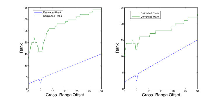
Figure 13: Computed and estimated rank of matrix $C$ for two stationary targets. One is fixed at location $\vec{\boldsymbol{\rho}}_{1}=(5,5,0)$m and the location of the other varies on the line segment between $(-5,0.01,0)$m and $(-5,30,0)$m.

4.5 Discussion

The analysis above shows that the matrix of data traces from a moving target has much higher rank than that from a stationary target. The larger the speed, the higher the rank. The rank of the matrix of traces from a stationary target is smallest, equal to one, when the target is at the same cross-range as the reference point $\vec{\boldsymbol{\rho}}_{o}$. The rank increases at a linear rate with the cross-range offset from $\vec{\boldsymbol{\rho}}_{o}$.

Comparing the results for one and two stationary targets, we see that the rank increases. The rank depends strongly on the cross-range offset of the targets. There is a small effect due to the separation of the targets in range, but it becomes negligible in the asymptotic limit $n\to\infty$.

Although we have not presented an analysis for more than two targets, we observe numerically that the rank increases as we add more and more stationary targets. The implication is that the matrix of traces from a stationary scene with many targets is not in general low rank. This is why the data separation with robust PCA should be done in successive small time windows, with each window containing the traces from only a few stationary targets. These traces give a matrix that is low rank, and thus can be separated from the traces due to moving targets. The simulation results shown in Figure 6 illustrate this point.

5 Numerical simulations

We begin with the setup for the numerical simulations. Then we present three sets of results.

5.1 Setup

We use the GOTCHA Volumetric SAR setup described in section (4.1). The data traces are generated with the model (4.5). In all the simulations but the last one, the point targets are assumed identical, with reflectivity $\sigma_{q}=1$. The images are obtained by computing the function (2.6) at points in the square imaging region of area $70\times 70\,\mbox{m}^{2}$ centered at $\vec{\boldsymbol{\rho}}_{o}$. The motion estimation results are obtained with the phase space algorithm introduced in [2]. This algorithm requires that we know the location of the target at one instant. We choose it at the center of the aperture, which is why there is no error in the target trajectory at $s=0$.

The principle component pursuit optimization in the robust PCA is solved with an augmented Lagrangian approach. It requires the computation of the top few singular values and corresponding singular vectors of large and sparse matrices, which we do with the software package PROPACK.

5.2 Simulation 1

The first simulation is for a collection of $30$ stationary targets placed randomly in the imaging region, and a single moving target located at $(0,0,0)$m at $s=0$, and moving in the plane with velocity ${\bf u}=\frac{28}{\sqrt{2}}(1,1)$m/s. The data traces are shown in Figure 5.

The estimated moving target trajectory is shown in the left plot in Figure 14. The blue line corresponds to the true trajectory. The red and green lines are the estimated trajectories with the sparse component of the matrix of traces, as returned by robust PCA with and without windowing. These sparse components are shown in the right plots in Figure 6. The separation with robust PCA is better for the windowed traces, and so is the estimate of the target trajectory. This is more clear in the rig ht plot of Figure 14, where we show the error of the trajectory.

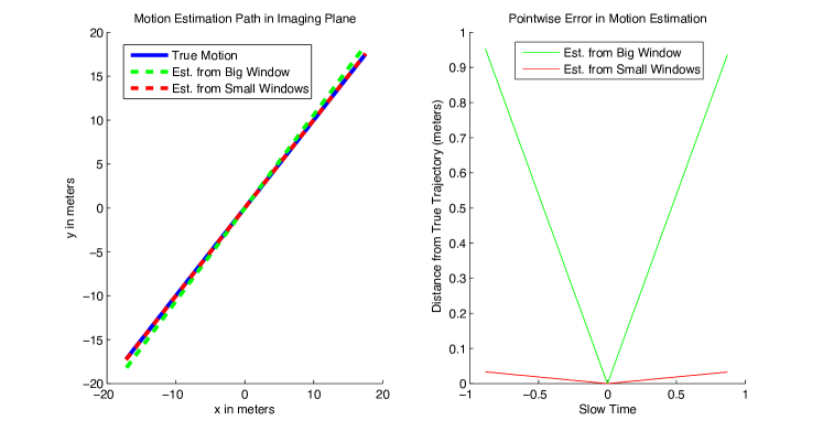
Figure 14: Estimation of the trajectory of a moving target in a complex scene with 30 stationary scatterers, placed at random in a $50\times 50\ m^{2}$ imaging region. We compare the results obtained with the sparse part of the data traces returned by robust PCA with and without windowing. These sparse parts are shown in the top right and bottom right plots in 6.

In the left plot of Figure 15 we show the image obtained with the data traces, and with exact compensation of the motion of the target. The image is focused at the initial location $(0,0,0)$m of the moving target, as expected. However, the stationary targets are out of focus, and the image appears noisy. The right plot of Figure 15 shows the image obtained with the sparse component of the traces, separated successfully by robust PCA with data windowing. The motion compensation is with the estimated velocity. We note that the artifacts due to the stationary targets are now removed, and the image peaks at the expected location $(0,0,0)$m. There are two ghost peaks, due to the error in the estimated target velocity, but they are much smaller than the peak at the correct location.

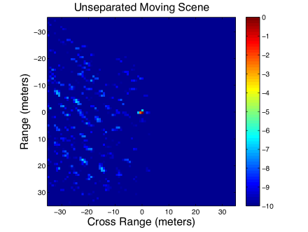
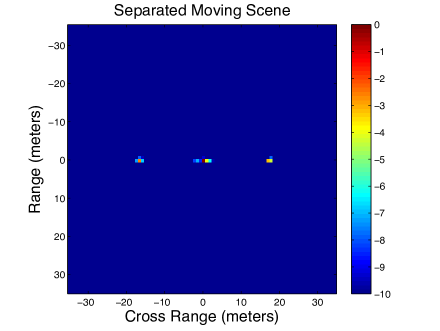
Figure 15: Images of a scene with 30 randomly placed stationary scatterers and one moving target with velocity 28 m/s. Left: the image given by the original data with exact compensation of the motion of the target. Right: the image given by the sparse component of the data, separated from the other traces by robust PCA with time windowing. The images are normalized by the largest pixel value and plotted in dB.

5.3 Simulation 2

The second simulation is for a scene with 20 stationary targets and two moving targets. The first moving target is as in the first simulation, The second one is located at $(-5,5,0)$m at $s=0$ and moves in the plane with velocity ${\bf u}=\frac{14}{\sqrt{3}}\left(-1,\sqrt{2}\right)$m/s.

The data traces $D_{r}(s,t)$ are plotted on the left in Figure 16. The separation with robust PCA is shown in the middle and right plots of Figure 16. Each is normalized by the maximum of $|D_{r}(s,t)|$, and then plotted on the same color scale. Note how the traces from the two moving targets are separated from the other traces. This simplifies the motion estimation.

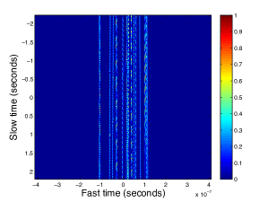
Figure 16: Data trace separation with robust PCA for a scene with 20 stationary targets and two moving targets. From left to right we show the matrix $M$ of data traces, the low rank ${\cal L}$, and the sparse ${\cal S}$ parts. In each plot we show absolute values normalized by the largest value of $|D_{r}(s,t)|$. The sparse component is plotted in dB scale to emphasize the contrast.

5.4 Simulation 3

Our last simulation considers again a scene with 30 stationary targets and a single moving target. This target is like that in simulation one, except that its reflectivity is ten times larger than that of the stationary targets.

The data separation results are in Figure 17. We show in Figure 18 the estimated target trajectory with the original data traces (left plot in Figure 17), and the sparse component (right plot in Figure 17). We obtain as before that the estimation is better after the data separation.

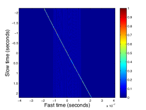
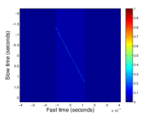
Figure 17: Data trace separation with robust PCA for a scene with 30 stationary targets and a moving one with reflectivity that is ten times stronger than the others. From left to right we show the matrix $M$ of data traces, the low rank ${\cal L}$, and the sparse ${\cal S}$ parts. In each plot we show absolute values normalized by the largest value of $|D_{r}(s,t)|$. The sparse component is plotted in dB scale to emphasize the contrast.

The left plot in Figure 19 shows the image computed with the original SAR data traces. The image is focused at the stationary targets, but there is a strong artifact (streak), due to the moving target. The middle plot in Figure 19 shows the image computed with the low rank component of the data traces, displayed in the middle in Figure 17. The effect of the moving target is now considerably smaller. The right plot in Figure 19 shows the image obtained with the sparse component of the traces, with motion compensation using the estimated target velocity. There is no artifact due to the stationary targets and the image is focused at the location $(0,0,0)$m, as expected.

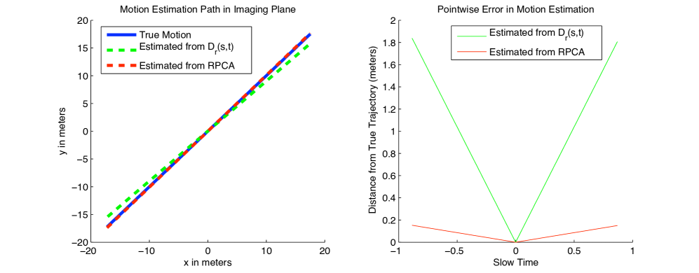
Figure 18: Estimation of the trajectory of a moving target in a complex scene with 30 stationary scatterers, placed at random in a $50\times 50\ m^{2}$ imaging region. The reflectivity of the moving target is ten times stronger than that of the stationary ones. Left: estimated target trajectory using the original traces (green) and the separated traces (red). The true trajectory is in blue. Right: errors of the estimated trajectories.

Figure 19: Images of a scene with 30 stationary targets and a moving one with reflectivity that is ten times stronger than the others. Left: image obtained with the original data traces. Middle: image obtained with the low rank component of the data traces, returned by robust PCA. Right: image obtained with the sparse component of the data traces, returned by robust PCA. The motion compensation is with the estimated target velocity.

6 Summary

In this paper we consider the problem of synthetic aperture radar (SAR) imaging of complex scenes consisting of a few moving and many stationary targets. The SAR setup is the usual one with a single antenna mounted on a platform flying above the region to be imaged. With large bandwidth probing signals and long data acquisition trajectories, SAR can produce high resolution images of stationary scenes. However, the presence of moving targets may cause serious degradation of the images. When the targets have moderate speed, they appear displaced and blurred in the images. Fast moving targets create significant artifacts such as prominent streaks.

To bring the images of the moving targets in focus we need to estimate their motion. This is necessarily done with small successive sub-apertures, corresponding to short acquisition times over which the target motion can be approximated by uniform translation. Imaging with motion estimation is difficult for at least the following reasons: First, the echoes from the moving targets may be overwhelmed by those from the stationary scenes, so the targets may be difficult to detect. Second, even if we can detect the presence of a moving target in a complex scene, it is difficult to estimate its motion with the existing algorithms, unless we use multiple receiver or transmitter antennas. The algorithms that work with the usual SAR setup assume that all the targets move the same way and are sensitive to the presence of strong stationary targets. Third, even if we detect and estimate well the target motion, when we compensate for it in the image formation process we may bring the stationary targets out of focus, and thus still get images with significant artifacts.

To address these challenges, we propose a pre-processing step of the SAR data designed to separate the stationary target echoes from those due to the moving targets. The main result of the paper is to show that this can be accomplished with the robust principal component analysis (PCA) algorithm complemented with appropriate data windowing. The robust PCA algorithm decomposes a matrix $M$ into a low rank part ${\cal L}$ and a sparse part ${\cal S}$. In our context, the matrix $M$ is given by the pulse and range compressed echoes received at the SAR platform. We show with analysis and numerical simulations that the contribution of the stationary targets to $M$ is a low rank matrix when we observe it in a small enough time window. Thus, we may think of it as the component ${\cal L}$ of $M$. The contribution of a few moving targets to $M$ is a sparse matrix that has higher rank, depending on the target velocity. Therefore, we expect that robust PCA separates it from the low rank part ${\cal L}$, due to the stationary targets.

We show with numerical simulations that indeed, robust PCA can accomplish such data separation. But the algorithm cannot be applied as a black box. It must be complemented with proper windowing of the pulse and range compressed SAR data in order to achieve a good separation. We present results for various imaging scenes containing multiple stationary targets, and one or two moving targets that may be stronger or weaker than the stationary ones. For weaker targets, we demonstrate that robust PCA can detect their faint echoes and it separates them from those due to the stationary targets. We also show motion estimation and imaging results with and without the data separation step, in order to demonstrate its importance in achieving good results.

Appendices

Appendix A Single target covariance matrix

We approximate here the function

$${\cal C}(s,s^{\prime}) \approx\frac{1}{\Delta t}\int_{-\infty}^{\infty}dt\,D_{r}(s,t)D_{r}(s^{\prime},t)$$

$$=\frac{1}{\Delta t}\int_{-\infty}^{\infty}dt\ \cos(\omega_{o}(t-\Delta\tau(s,\vec{\boldsymbol{\rho}}(s))))\exp\left[-\frac{B^{2}}{2}(t-\Delta\tau(s,\vec{\boldsymbol{\rho}}(s)))^{2}\right]$$

$$\hskip 43.36243pt\times\cos(\omega_{o}(t-\Delta\tau(s^{\prime},\vec{\boldsymbol{\rho}}(s^{\prime}))))\exp\left[-\frac{B^{2}}{2}(t-\Delta\tau(s^{\prime},\vec{\boldsymbol{\rho}}(s^{\prime})))^{2}\right],$$

and simplify notation as

$$\Delta\tau^{-}(s,s^{\prime}) :=\Delta\tau(s,\vec{\boldsymbol{\rho}}(s))-\Delta\tau(s^{\prime},\vec{\boldsymbol{\rho}}(s^{\prime}))$$

$$\Delta\tau^{+}(s,s^{\prime}) :=\Delta\tau(s,\vec{\boldsymbol{\rho}}(s))+\Delta\tau(s^{\prime},\vec{\boldsymbol{\rho}}(s^{\prime}))$$

We rewrite the integrand using a trigonometric identity, and completing the square

$$\cos[\omega_{o}(t-\Delta\tau(s,\vec{\boldsymbol{\rho}}(s)))]\cos[\omega_{o}(t-\Delta\tau(s^{\prime},\vec{\boldsymbol{\rho}}(s)))]\exp\left[-\frac{B^{2}}{2}(t-\Delta\tau(s,\vec{\boldsymbol{\rho}}(s)))^{2}-\frac{B^{2}}{2}(t-\Delta\tau(s,\vec{\boldsymbol{\rho}}(s)))^{2}\right]=$$

$$\frac{1}{2}\exp\left[-\frac{B^{2}\left(\Delta\tau^{-}(s,s^{\prime})\right)^{2}}{4}\right]\left\{\cos[\omega_{0}\Delta\tau^{-}(s,s^{\prime})]+\cos\left[2\omega_{o}\left(t+\frac{\Delta\tau^{+}(s,s^{\prime})}{2}\right)\right]\right\}$$

$$\times\exp\left[-B^{2}\left(t+\frac{\Delta\tau^{+}(s,s^{\prime})}{2}\right)^{2}\right],$$

and obtain that

$${\cal C}(s,s^{\prime}) = \frac{1}{2\Delta t}\cos[\omega_{0}\Delta\tau^{-}(s,s^{\prime})]\exp\left[-\frac{B^{2}\left(\Delta\tau^{-}(s,s^{\prime})\right)^{2}}{4}\right]\int_{-\infty}^{\infty}dt\ \exp\left[-B^{2}\left(t+\frac{\Delta\tau^{+}(s,s^{\prime})}{2}\right)^{2}\right]$$

$$+\frac{1}{2\Delta t}\exp\left[-\frac{B^{2}\left(\Delta\tau^{-}(s,s^{\prime})\right)^{2}}{4}\right]\int_{-\infty}^{\infty}dt\ \cos\left[2\omega_{o}\left(t+\frac{\Delta\tau^{+}(s,s^{\prime})}{2}\right)\right]\exp\left[-B^{2}\left(t+\frac{\Delta\tau^{+}(s,s^{\prime})}{2}\right)^{2}\right]$$

$$= \frac{\sqrt{\pi}}{2B\Delta t}\cos[\omega_{0}\Delta\tau^{-}(s,s^{\prime})]\exp\left[-\frac{B^{2}\left(\Delta\tau^{-}(s,s^{\prime})\right)^{2}}{4}\right]-\frac{\sqrt{\pi}}{2B\Delta t}\exp\left[-\frac{B^{2}\left(\Delta\tau^{-}(s,s^{\prime})\right)^{2}}{4}-\frac{\omega_{o}^{2}}{B^{2}}\right]$$

$$\approx \frac{\sqrt{\pi}}{2B\Delta t}\cos[\omega_{0}\Delta\tau^{-}(s,s^{\prime})]\exp\left[-\frac{B^{2}\left(\Delta\tau^{-}(s,s^{\prime})\right)^{2}}{4}\right].$$

The last approximation is because in our regime $\omega_{o}\gg B$.

Our assumption (4.16) on the Fresnel number, and therefore on the aperture, allows us to linearize $\Delta\tau^{-}(s,s^{\prime})$ and obtain the Toeplitz structure stated in Proposition 1. We have by the mean value theorem that

$$\Delta\tau^{-}(s,s^{\prime})=(s-s^{\prime})\frac{d}{ds}\Delta\tau(\bar{s},\vec{\boldsymbol{\rho}}(\bar{s}))$$ (A.1)

for some $\bar{s}$ between $s$ and $s^{\prime}$. The derivative is given by

$$\frac{d}{ds}\Delta\tau(\bar{s},\vec{\boldsymbol{\rho}}(\bar{s}))=\frac{2}{c_{o}}\left[V\vec{{\bf t}}(\bar{s})\cdot\left(\vec{{\bf m}}(\bar{s})-\vec{{\bf m}}_{o}(\bar{s})\right)-\vec{\bf u}\cdot\vec{{\bf m}}(\bar{s})\right],$$ (A.2)

in terms of the unit vectors

$$\vec{{\bf m}}(\bar{s})=\frac{\vec{\bf r}(\bar{s})-\vec{\boldsymbol{\rho}}(\bar{s})}{|\vec{\bf r}(\bar{s})-\vec{\boldsymbol{\rho}}(\bar{s})|},\quad\vec{{\bf m}}_{o}(\bar{s})=\frac{\vec{\bf r}(\bar{s})-\vec{\boldsymbol{\rho}}_{o}}{|\vec{\bf r}(\bar{s})-\vec{\boldsymbol{\rho}}_{o}|},$$

and the unit vector $\vec{{\bf t}}(\bar{s})$ tangential to the flight path at $\vec{\bf r}(\bar{s})$. We use that

$$\vec{{\bf m}}(\bar{s})-\vec{{\bf m}}_{o}(\bar{s})=\left[I-\vec{{\bf m}}_{o}(\bar{s})\vec{{\bf m}}_{o}(\bar{s})^{T}\right]\frac{(\vec{\boldsymbol{\rho}}(\bar{s})-\vec{\boldsymbol{\rho}}_{o})}{|\vec{\bf r}(\bar{s})-\vec{\boldsymbol{\rho}}_{o}|}+O\left[\left(\frac{R^{{}^{\cal I}}}{L}\right)^{2}\right],$$

and expand the right hand side in (A.2) around $\bar{s}=0$ and obtain

$$\frac{d}{ds}\Delta\tau(\bar{s},\vec{\boldsymbol{\rho}}(\bar{s}))=\frac{2}{c_{o}}\left[V\vec{{\bf t}}\cdot\frac{\mathbb{P}_{o}(\vec{\boldsymbol{\rho}}-\vec{\boldsymbol{\rho}}_{o})}{|\vec{\bf r}(0)-\vec{\boldsymbol{\rho}}_{o}|}-\vec{\bf u}\cdot\vec{{\bf m}}_{o}-\vec{\bf u}\cdot\frac{\mathbb{P}_{o}(\vec{\boldsymbol{\rho}}-\vec{\boldsymbol{\rho}}_{o})}{|\vec{\bf r}(0)-\vec{\boldsymbol{\rho}}_{o}|}\right]+O\left(\frac{a\vec{{\bf t}}\cdot\mathbb{P}_{o}\vec{\bf u}}{c_{o}L}\right)+O\left(\frac{VaR^{{}^{\cal I}}}{c_{o}L^{2}}\right).$$ (A.3)

Therefore,

$$\omega_{o}\Delta\tau^{-}(s,s^{\prime})=\frac{2(s-s^{\prime})}{c_{o}}\left[V\vec{{\bf t}}\cdot\frac{\mathbb{P}_{o}(\vec{\boldsymbol{\rho}}-\vec{\boldsymbol{\rho}}_{o})}{|\vec{\bf r}(0)-\vec{\boldsymbol{\rho}}_{o}|}-\vec{\bf u}\cdot\vec{{\bf m}}_{o}-\vec{\bf u}\cdot\frac{\mathbb{P}_{o}(\vec{\boldsymbol{\rho}}-\vec{\boldsymbol{\rho}}_{o})}{|\vec{\bf r}(0)-\vec{\boldsymbol{\rho}}_{o}|}\right]+\mathcal{E},$$ (A.4)

with negligible error by assumption (4.16)

$$\mathcal{E}=O\left(\frac{a^{2}\vec{{\bf t}}\cdot\mathbb{P}_{o}\vec{\bf u}}{\lambda_{o}LV}\right)+O\left(\frac{a^{2}R^{{}^{\cal I}}}{\lambda_{o}L^{2}}\right)\ll 1.$$

This is the result stated in Proposition 1.

Appendix B Computation of the symbol

The symbol is given by

$$Q(\theta)=\sum_{j=-\infty}^{\infty}c_{j}e^{ij\theta},\quad\quad\theta\in(-\pi,\pi)$$ (B.1)

with $c_{j}$ defined by (4.24). Thus

$$Q(\theta) =\frac{\sqrt{\pi}}{2B\Delta t}\sum_{j=-\infty}^{\infty}e^{-\frac{(\xi j)^{2}}{4}}\cos(\gamma j)e^{ij\theta}$$

$$=\frac{\sqrt{\pi}}{2B\Delta t}\left(\sum_{j=-\infty}^{\infty}\left[\cos(j\theta)\cos(\gamma j)e^{-\frac{(\xi j)^{2}}{4}}\right]+i\sum_{j=-\infty}^{\infty}\left[\sin(n\theta)\cos(\gamma j)e^{-\frac{(\xi j)^{2}}{4}}\right]\right)$$

$$=\frac{\sqrt{\pi}}{4B\Delta t}\sum_{j=-\infty}^{\infty}\left[\cos(n(\theta-\gamma))+\cos(n(\theta+\gamma))\right]e^{-\frac{(\xi j)^{2}}{4}},$$

where we recall that

$$\xi=B|\alpha|\Delta s.$$

Define $\Delta x=\xi/2$ and $x_{j}=j\Delta x$. Then

$$Q(\theta) =\frac{\sqrt{\pi}}{4B\Delta t}\frac{1}{\Delta x}\sum_{j=-\infty}^{\infty}\left[\cos\left(\frac{2(\theta-\gamma)}{\xi}x_{j}\right)+\cos\left(\frac{2(\theta+\gamma)}{\xi}x_{j}\right)\right]e^{-x_{j}^{2}}\Delta x$$

For $\theta\in(-\pi,\pi)$ and $\xi$ (i.e., $\Delta s$) small enough, we can approximate the sum with an integral

$$Q(\theta) \approx\frac{\sqrt{\pi}}{2B\Delta t\xi}\int_{-\infty}^{\infty}\left[\cos\left(\frac{2(\theta-\gamma)}{\xi}x\right)+\cos\left(\frac{2(\theta+\gamma)}{\xi}x\right)\right]e^{-x^{2}}dx$$

$$=\frac{\pi}{2B\Delta t\xi}\left[e^{-\frac{(\theta-\gamma)^{2}}{\xi^{2}}}+e^{-\frac{(\theta+\gamma)^{2}}{\xi^{2}}}\right].$$

Appendix C Rank estimate of large Toeplitz plus g-Hankel matrices

We use the results from [19] to obtain the asymptotic estimate of the rank of matrix $C$ given by equation (4.37) as the sum of a Toeplitz matrix $T$, a g-Hankel matrix $H$ and its transpose. We need the following definition:

Definition 2

Let $Q$ be a complex valued, measurable function defined on the interval $U=(-\pi,\pi)$. Let also $\{A_{n}\}_{n\in\mathbb{N}}$ be a sequence of of matrices. Each matrix $A_{n}\in\mathbb{R}^{(n+1)\times(n+1)}$, and we denote by $\sigma_{j}(A_{n})$ its singular values, in descending order, for $j=1,\ldots,n+1$. We say that the sequence is distributed (in the sense of singular values) as the pair $(Q,U)$, and write in short $\{A_{n}\}\sim_{\sigma}(Q,U)$, if

$$\lim_{n\to\infty}\frac{1}{n+1}\sum_{j=1}^{n+1}F(\sigma_{j}(A_{n}))=\frac{1}{2\pi}\int_{-\pi}^{\pi}F(|Q(\theta)|)d\theta,$$ (C.1)

for every $F\in C_{o}(\mathbb{R}^{+})$. Here $C_{o}(\mathbb{R}^{+})$ is the set of continuous functions with bounded support over the nonnegative real numbers.

It is shown in [19, section 4.2.2] that if $\{H_{n}\}_{n\in\mathbb{N}}$ is a sequence of g-Hankel matrices $H_{n}\in\mathbb{R}^{(n+1)\times(n+1)}$, then

$$\{H_{n}\}\sim_{\sigma}(0,U).$$ (C.2)

Moreover, [19, Proposition 4.3] states that if $\{A_{n}\}_{n\in\mathbb{N}}$ and $\{H_{n}\}_{n\in\mathbb{N}}$ are two sequences of matrices satisfying $\{A_{n}\}\sim_{\sigma}(Q,U)$ and $\{H_{n}\}\sim_{\sigma}(0,U)$ then

$$\{A_{n}+H_{n}\}\sim_{\sigma}(Q,U).$$ (C.3)

In our context, $A_{n}=T_{n}$ are Toeplitz matrices defined by the sequence $\{c_{j}\}_{j\in\mathbb{Z}}$, and $Q$ is the symbol defined by (4.26). We are interested in the distribution (in the sense of singular values) of the sequence $\{C_{n}\}_{n\in\mathbb{N}}$ defined by

$$C_{n}=T_{n}+H_{n}+H_{n}^{T}.$$ (C.4)

Because the singular values of the transpose $H_{n}^{T}$ are the same as the singular values of $H_{n}$, we obtain using (C.2) and Definition (2) that

$$\{H_{n}^{T}\}\sim_{\sigma}(0,U).$$ (C.5)

Thus, $\{(T_{n}+H_{n})+H_{n}^{T}\}$ has the same distribution as $\{T_{n}+H_{n}\}$ and by (C.3),

$$\{T_{n}+H_{n}\}\sim_{\sigma}(Q,U).$$ (C.6)

More explicitly,

$$\lim_{n\to\infty}\frac{1}{n+1}\sum_{j=1}^{n+1}F(\sigma_{j}(T_{n}+H_{n}+H_{n}^{T}))=\frac{1}{2\pi}\int_{-\pi}^{\pi}F(|Q(\theta)|)d\theta,\qquad\forall F\in C_{0}(\mathbb{R}^{+}).$$ (C.7)

We cannot apply directly this result to the computation of rank, because the indicator function $1_{[\epsilon\|Q\|_{\infty},\infty)}$ does not have bounded support and it is not continuous. However, the result extends to such functions as we shown next.

First, let us show that the sigular values of matrices $T_{n}+H_{n}$ are bounded uniformly in $n$. Because the largest singular value of a matrix is equal to its 2-norm, we obtain by the triangle inequality that

$$\sigma_{1}(T_{n}+H_{n}+H_{n}^{T})=\|T_{n}+H_{n}+H_{n}^{T}\|_{2}\leq\|T_{n}\|_{2}+2\|H_{n}\|_{2}=\sigma_{1}(T_{n})+2\sigma_{1}(H_{n}).$$

One of the results of the Szegő theory for large Toeplitz matrices [17, 3] is that the sequence of largest singular values $\{\sigma_{1}(T_{n})\}_{n\in\mathbb{N}}$ converges to the limit $\|Q\|_{\infty}$. Thus, the sequence is bounded above, and we denote the bound by $\Sigma_{T}$. For the g-Hankel matrix we can use the matrix norm inequality

$$\sigma_{1}(H_{n})=\|H_{n}\|_{2}\leq\sqrt{\|H_{n}\|_{1}\|H_{n}\|_{\infty}},$$

where $\|H_{n}\|_{1}$ and $\|H_{n}\|_{\infty}$ are equal to the maximum of the 1-norm of the columns and rows of $H_{n}$, respectively. They are defined by equation (4.39), in terms of the sequence $\{h_{j}\}$ given in equation (4.41). Obviously, the 1-norm of the columns and rows of $H_{n}$ are bounded above by the series

$$\Sigma_{H}=\sum_{j=0}^{\infty}|h_{j}|<\infty,$$

which is convergent because $h_{j}$ decays exponentially with $j$. Therefore,

$$\|H_{n}\|_{1}\leq\Sigma_{H}\quad\mbox{and}\quad\|H_{n}\|_{\infty}\leq\Sigma_{H}$$

and gathering the results above, we have that

$$\sigma_{1}(T_{n}+H_{n})\leq\Sigma_{T}+2\Sigma_{H}.$$ (C.8)

Since the singular values are bounded by (C.8), in our calculation of rank we can replace the indicator function $1_{[\epsilon\|Q\|_{\infty},\infty)}(x)$ with a new function $\chi(x)$ of bounded support, satisfying

$$\chi(x)=\begin{cases}0&~{}~{}x<\delta,\\ 1&~{}~{}x\in[\delta,D],\end{cases}$$ (C.9)

and decaying to zero in a continuum manner for $x>D$. Here we simplified notation as

$$\delta:=\epsilon\|Q\|_{\infty}\quad\mbox{and}\quad D=\Sigma_{T}+2\Sigma_{H}.$$

It remains to show that result (C.7) extends to the function $\chi$, which has bounded support but is discontinuous at $x=\delta$.

Let us introduce the sequence of continuous functions $\{\chi_{m}(x)\}_{m\in\mathbb{Z}^{+}}$, defined by

$$\chi_{m}(x)=\begin{cases}0&~{}~{}x<\delta-\frac{1}{m}\\ m(x-\delta)+1&\delta-\frac{1}{m}\leq x\leq\delta\\ \chi(x)&~{}~{}x>\delta.\end{cases}$$ (C.10)

This sequence converges pointwise to $\chi(x)$, as $m\to\infty$. We know that (C.7) holds for $F=\chi_{m}$. To extend the result to $F=\chi$, we show next that we can interchange the limits as in

$$\lim_{m\to\infty}\lim_{n\to\infty}\frac{1}{n+1}\sum_{j=1}^{n+1}\chi_{m}\left(\sigma_{j}(T_{n}+H_{n}+H_{n}^{T})\right) =\lim_{n\to\infty}\lim_{m\to\infty}\frac{1}{n+1}\sum_{j=1}^{n+1}\chi_{m}\left(\sigma_{j}(T_{n}+H_{n}+H_{n}^{T})\right)$$

$$=\lim_{n\to\infty}\frac{1}{n+1}\sum_{j=1}^{n+1}\chi\left(\sigma_{j}(T_{n}+H_{n}+H_{n}^{T})\right).$$

We have that

$$\lim_{m\to\infty}\lim_{n\to\infty}\frac{1}{n+1}\sum_{j=1}^{n+1}\chi_{m}\left(\sigma_{j}(T_{n}+H_{n}+H_{n}^{T})\right)-\lim_{n\to\infty}\frac{1}{n+1}\sum_{j=1}^{n+1}\chi\left(\sigma_{j}(T_{n}+H_{n}+H_{n}^{T})\right)$$

$$=\lim_{m\to\infty}\left[\lim_{n\to\infty}\frac{1}{n+1}\sum_{j=1}^{n+1}\left[\chi_{m}\left(\sigma_{j}(T_{n}+H_{n}+H_{n}^{T})\right)-\chi\left(\sigma_{j}(T_{n}+H_{n}+H_{n}^{T})\right)\right]\right]$$

$$=\lim_{m\to\infty}\left[\lim_{n\to\infty}\frac{1}{n+1}\sum_{j=1}^{n+1}\left[g_{m}\left(\sigma_{j}(T_{n}+H_{n}+H_{n}^{T})\right)\right]\right]$$ (C.11)

with residual $g_{m}:=\chi_{m}-\chi$ that satisfies by construction

$$g_{m}(x)\geq 0,\qquad\forall x\in\mathbb{R},$$

and is bounded above by the continous function

$${\mathcal{G}}_{m}(x)=\begin{cases}0&x<\delta-\frac{1}{m}\\ m(x-\delta)+1&\delta-\frac{1}{m}\leq x\leq\delta\\ -m(x-\delta)+1&\delta<x\leq\delta+\frac{1}{m}\\ 0&x>\delta+\frac{1}{m}.\end{cases}$$

This gives

$$0\leq\lim_{m\to\infty}\left[\lim_{n\to\infty}\frac{1}{n+1}\sum_{j=1}^{n+1}\left[g_{m}\left(\sigma_{j}(T_{n}+H_{n}+H_{n}^{T})\right)\right]\right] \leq\lim_{m\to\infty}\left[\lim_{n\to\infty}\frac{1}{n+1}\sum_{j=1}^{n+1}\left[{\mathcal{G}}_{m}\left(\sigma_{j}(T_{n}+H_{n}+H_{n}^{T})\right)\right]\right]$$

$$=\lim_{m\to\infty}\frac{1}{2\pi}\int_{-\pi}^{\pi}{\mathcal{G}}_{m}\left(Q(\theta)\right)d\theta,$$

and we can bring the limit inside the integral using the dominated convergence theorem

$$\lim_{m\to\infty}\frac{1}{2\pi}\int_{-\pi}^{\pi}{\mathcal{G}}_{m}\left(Q(\theta)\right)d\theta=\frac{1}{2\pi}\int_{-\pi}^{\pi}\lim_{m\to\infty}{\mathcal{G}}_{m}\left(Q(\theta)\right)d\theta=0.$$

The last equality is because ${\mathcal{G}}_{m}\to 0$ almost everywhere. Thus, the limit (C.11) is equal to zero, and the result follows.

References

- [1] S. Barbarossa and A. Farina. Detection and imaging of moving objects with synthetic aperture radar. IEE Proceedings-F, 139(1):79–88, 1992.
- [2] L. Borcea, T. Callaghan, and G. Papanicolaou. Synthetic Aperture Radar Imaging with Motion Estimation and Autofocus. Inverse Problems, 28:045006, 2012.
- [3] A. Böttcher and B. Silbermann. Introduction to Large Truncated Toeplitz Matrices. Springer, 1999.
- [4] E. J. Candès, X. Li, Y. Ma, and J. Wright. Robust Principal Component Analysis? Journal of ACM, 58(1):1–37, 2009.
- [5] C.H. Casteel Jr, L.R.A. Gorham, M.J. Minardi, S.M. Scarborough, K.D. Naidu, and U.K. Majumder. A challenge problem for 2d/3d imaging of targets from a volumetric data set in an urban environment. In Proceedings of SPIE, volume 6568, page 65680D, 2007.
- [6] M. Cheney. A mathematical tutorial on synthetic aperture radar. SIAM review, 43(2):301–312, 2001.
- [7] John C. Curlander and Robert N. McDonough. Synthetic Aperture Radar: Systems and Signal Processing. Wiley-Interscience, 1991.
- [8] Y. Ding and DC Munson Jr. Time-frequency methods in SAR imaging of moving targets. In IEEE International Conference on Acoustics, Speech, and Signal Processing, 2002. Proceedings.(ICASSP’02), volume 3, pages 2881–2884, 2002.
- [9] Y. Ding, N. Xue, and DC Munson Jr. An analysis of time-frequency methods in SAR imaging of moving targets. In Sensor Array and Multichannel Signal Processing Workshop. 2000. Proceedings of the 2000 IEEE, pages 221–225, 2000.
- [10] J. Ender. Detectability of slowly moving targets using a multi-channel SAR with an along-track antenna array. In Proceedings of SEE/IEE Conference (SAR 93), Paris, pages 19–22, 1993.
- [11] D. Fasino. Spectral properties of Toeplitz-plus-Hankel matrices. Calcolo, 33:87–98, 1996.
- [12] D. Fasino and P. Tilli. Spectral clustering properties of block multilevel Hankel matrices. Linear Algebra and its Applications, 306:155–163, 2000.
- [13] J. R. Fienup. Detecting Moving Targets in SAR Imagery by Focusing. IEEE Transactions on Aerospace and Electronic Systems, 37(3):794–809, 2001.
- [14] B. Friedlander and B. Porat. VSAR: a high resolution radar system for detection of moving targets. IEE Proc.-Radar, Sonar Navig., 144(4):205–218, 1997.
- [15] J. K. Jao. Theory of Synthetic Aperture Radar Imaging of a Moving Target. IEEE Transactions on Geoscience and Remote Sensing, 39(9):1984–1992, 2001.
- [16] Charles V. Jakowatz Jr., Daniel E. Wahl, Paul H. Eichel, Dennis C. Ghiglia, and Paul A. Thompson. Spotlight-mode synthetic aperture radar: A signal processing approach. Springer, New York, NY, 1996.
- [17] M. Kac, W. L. Murdock, and G. Szegő. On the eigenvalues of certain Hermitian forms. J. Rational Mech. Anal., (1):767–800, 1953.
- [18] M. Kirscht. Detection and imaging of arbitrarily moving targets with single-channel SAR. IEE Proc.-Radar Sonar Navig., 150(1):1984–1992, 2003.
- [19] E. Ngondiep, S Serra-Capizzano, and D. Sesana. Spectral Features and Asymptotic Properties for -Circulants and -Toeplitz Sequences. SIAM J. Matrix Anal. Appl., 31(4):1663–1687, 2010.
- [20] R. P. Perry, R. C. DiPietro, and R. L. Fante. SAR Imaging of Moving Targets. IEEE Transactions on Aerospace and Electronic Systems, 35(1):188–200, 1999.
- [21] T. Sparr. Time-Frequency Signatures of a Moving Target in SAR Images. Paper presented at the RTO SET Symposium on Target Identification and Recognition Using RF Systems, Oslo, Norway, 11-13 October, 2004. Published in RTO-MP-SET-080.
- [22] G. Wang, X. Xia, and V. Chen. Dual-Speed SAR Imaging of Moving Targets. IEEE Transactions on Aerospace and Electronic Systems, 42(1):368–379, 2006.
- [23] G. Wang, X. Xia, V. Chen, and R. Fiedler. Detection, Location, and Imaging of Fast Moving Targets Using Multifrequency Antenna Array SAR. IEEE Transactions on Aerospace and Electronic Systems, 40(1):345–355, 2004.
- [24] S. Zhu, G. Liao, Y. Qu, Z. Zhou, and X. Liu. Ground Moving Targets Imaging Algorithm for Synthetic Aperture Radar. IEEE Transactions on Geoscience and Remote Sensing, 49(1):462–477, 2011.