Maximum intrinsic spin-Hall conductivity in two-dimensional systems with k-linear spin-orbit interaction

Abstract

We analytically calculate the intrinsic spin-Hall conductivity (ISHC) ($\sigma^{z}_{xy}$ and $\sigma^{z}_{yx}$) in a clean, two-dimensional system with generic k-linear spin-orbit interaction. The coefficients of the product of the momentum and spin components form a spin-orbit matrix $\widetilde{\beta}$. We find that the determinant of the spin-orbit matrix $\mathrm{det}\widetilde{\beta}$ describes the effective coupling of the spin $s_{z}$ and orbital motion $L_{z}$. The decoupling of spin and orbital motion results in a sign change of the ISHC and the band-overlapping phenomenon. Furthermore, we show that the ISHC is in general unsymmetrical ($\sigma^{z}_{xy}\neq-\sigma^{z}_{yx}$), and it is governed by the asymmetric response function $\Delta\widetilde{\beta}$, which is the difference in band-splitting along two directions: those of the applied electric field and the spin-Hall current. The obtained non-vanishing asymmetric response function also implies that the ISHC can be larger than $e/8\pi$, but has an upper bound value of $e/4\pi$. We will that the unsymmetrical properties of the ISHC can also be deduced from the manifestation of the Berry curvature at the nearly degenerate area. On the other hand, by investigating the equilibrium spin current, we find that $\mathrm{det}\widetilde{\beta}$ determines the field strength of the SU(2) non-Abelian gauge field.

I Introduction

Within condensed matter physics, spintronics has in itself become a strong field for considerable research, owing to not only its potential applications in electronic technologies but also the many fundamental questions that are raised on the physics of electron spin. pri98 Particularly, the spin-orbit interaction recently has strongly attracted the attentions of theoreticians and experimenters since it opens up the possibility of manipulating electron (or hole) spin in non-magnetic materials by electrical means. zut04 ; Hisch99 Since the theoretical prediction of the spin-Hall effect, the application of spintronics has seen considerable advancement. It was shown that the Mott-type skew scattering by impurities would result in separation of opposite spin states via the spin-orbit interaction to the impurity atom. Hisch99 This is the extrinsic spin-Hall effect. Nevertheless, it has been found that in p-type Murakami03 (Luttinger model) and n-type Sinova04 (Rashba model) semiconductors, the spin-polarized current (electron or hole) can be generated by the intrinsic spin-orbit interaction in non-magnetic structure in the absence of impurity scattering, which is called the intrinsic spin-Hall effect (ISHC).

The calculation of spin-Hall conductivity (SHC) plays a crucial role in studying the spin-Hall effect as it can be in comparison with experimental result. The extrinsic spin-Hall effect was experimentally discovered in the three-dimensional (3D) n-type GaAs by optical means via spin accumulation at the edges of a sample Kato04 ; Stern06 and in two-dimensional (2D) n-type AlGaAs/GaAs. Sih05 The magnitude of the experimental value of SHC [$0.5(1/em\Omega)$] in Ref. Kato04 agrees with its theoretical value [$0.9(1/em\Omega)$]. Engel05 However, the sign of the theoretical SHC is opposite to the experimental value, and it needs to be further clarified. Engel05 In 2D p-type AlGaAs/GaAs Wund05 , the experimental value of SHC [$2.5(e/8\pi)$] also agrees with the theoretical value [$1.9(e/8\pi)$] in order of magnitude. Berne05 . Particularly, in Ref. Berne05 , the clean limit is considered in the calculation. In 2D n-type InGaN/GaN, the strain-dependent intrinsic spin-Hall effect detected by optical means is explained in terms of SHC in which the strain effect is included. Chang06 In 3D metal Pt wire, the large ISHC measured electrically throughout the inverse spin-Hall effect at room temperature is $240(\hbar/e\Omega cm)$. Saitoh06 ; Kimura07 It was theoretically explained in Ref. Guo08 on the basis of the huge Berry curvature boh03 near the Fermi level at the L and X symmetry point in the Pt Brillouin zone; the obtained theoretical value of ISHC is $200(\hbar/e\Omega cm)$ in the absence of impurity scattering. Most recently, a large spin-Hall signal is observed at room temperature in FePt/Au multi-terminal devices. Seki08

Importantly, both the direction of the applied electric field and the strength of the spin-orbit interactions alters the values of the ISHC. For the former case, a typical example is the Rashba-Dresselhaus system. RD When an electric field is applied along the $x$ ($[010]$) (or $y$ $[100]$) direction, we obtain $\sigma^{z}_{xy}=-\sigma^{z}_{yx}$, and these values are equal to the universal constant $e/8\pi$. However, if an electric field is applied along $x^{\prime}$ ($[110]$) (or $y^{\prime}$, i.e., $[1\bar{1}0]$), we obtain $\sigma^{z}_{x^{\prime}y^{\prime}}\neq-\sigma^{z}_{y^{\prime}x^{\prime}}$, and one of these values has a value higher than $e/8\pi$. The later case requires a systematical investigation because the spin-orbit interaction could be very complicated. For example, it has been proposed that a strained semiconductor results in various k-linear band-splitting. BernePRB05 Nevertheless, we find that strain-induced spin splitting together with the spin-orbit coupling of the host semiconductor can be simplified and expressed in terms of the coefficients of the spin-orbit matrix [see Eq. (2)]. In this study, we focus on generic 2D k-linear spin-orbit coupled systems without impurity scattering, and we systematically investigate the effects of spin-orbit interactions and the direction of the applied electric field on spin-Hall current. We find that the ISHC can be calculated analytically and that its unsymmetrical properties can be described using a unified approach.

We show that $\mathrm{det}\widetilde{\beta}$ [see Eq. (15)] is expressed as the effective coupling of the z-component of spin $s_{z}$, and orbital angular momentum $L_{z}$. The decoupling of spin and orbital motion associated with the band-overlapping phenomenon results in the vanishing and sign change of the ISHC.

Furthermore, by analytically calculating the ISHC, we find that the unsymmetrical result of the ISHC ($\sigma_{xy}^{z}\neq\sigma_{yx}^{z}$) is governed by the asymmetric response function $\Delta\widetilde{\beta}$ [see Eq. (30)], which is the difference in band-splitting in two directions: those of the applied electric field and the spin-Hall current. We find that the direction of the applied electric field alters the magnitude of the asymmetric response function. Consequently, we show that there exists a specific direction of applied electric field such that the asymmetric response function reaches a maximum value. In this case, we show that the ISHC also reaches a maximum value in the range $e/8\pi$ to $e/4\pi$, where $e/4\pi$ is the upper bound value of the ISHC. The unsymmetrical result and the maximum asymmetric response function of the ISHC can also be deduced from the behavior of the Berry curvature at the nearly degenerate area. The nearly degenerate area refers to the area where the inner and outer bands are very close to each other on the Fermi surface.

Our present paper is organized as follows. In Sec. II, we define the spin-orbit matrix obtained from the coefficients of the product of momentum and spin. The intrinsic spin-Hall conductivity is shown to be proportional to the determinant of spin-orbit matrix $\mathrm{det}\widetilde{\beta}$. We use Foldy-Wouthuysen transformation to show that the effective coupling of the spin $z$-component $s_{z}$ and orbital angular momentum $L_{z}$ is $-2m(\mathrm{det}\widetilde{\beta})/\hbar^{4}$. In Sec. III, we analytically calculate the ISHC of the generic 2D k-linear spin-orbit coupled system. The asymmetric response function and the upper bound value of ISHC will be discussed. In Sec. IV, in order to reveal the maximum value of ISHC, the direction of applied electric field and its influence on the asymmetric response function is studied. In Sec. V, we will show that the unsymmetrical properties of ISHC can be deduced from the variation of Berry curvature. In Sec. VI, we discuss the relationship between equilibrium spin current and spin-orbit matrix. We show that $\mathrm{det}\widetilde{\beta}$ plays the role of color magnetic field strength. Our conclusions are presented in Sec. VII.

II Intrinsic Spin-Hall conductivity

II.1 spin-orbit matrix and ISHC

The 2D k-linear spin-orbit coupled system Hamiltonian in the presence of an applied electric field can be written as

$$H=\varepsilon_{\mathbf{k}}+H_{so}+V(x,y),\\$$ (1)

where

$$\begin{split}H_{so}&=\sum_{ij}\beta_{ij}\sigma_{i}k_{j}\\ &=\left(\sigma_{x}~{}~{}\sigma_{y}\right)\left(\begin{array}[]{cc}\beta_{xx}&\beta_{xy}\\ \beta_{yx}&\beta_{yy}\end{array}\right)\left(\begin{array}[]{c}k_{x}\\ k_{y}\end{array}\right).\end{split}$$ (2)

The kinetic energy is $\varepsilon_{\mathbf{k}}=\hbar^{2}k^{2}/2m$ and $\sigma_{i}~{}(i=x,y)$ are the Pauli spin matrices. The external potential $V(x,y)$ is $V(x,y)=e\mathbf{E}\cdot\mathbf{x}$. The generic k-linear spin-orbit coupled 2D systems are related to the spin-orbit matrix $\widetilde{\beta}$,

$$\widetilde{\beta}=\left(\begin{array}[]{cc}\beta_{xx}&\beta_{xy}\\ \beta_{yx}&\beta_{yy}\end{array}\right),$$ (3)

where the coefficients $\beta_{ij}$ represent the spin-orbit interactions in 2D systems. As an example, consider the Rashba system [$\alpha(\sigma_{x}k_{y}-\sigma_{y}k_{x})$] BRashba , the pure Dresselhaus system [$-\beta(\sigma_{x}k_{x}-\sigma_{y}k_{y})$] Dre55 and the Dirac-type system [$g(\sigma_{x}k_{x}+\sigma_{y}k_{y})$] McClure56 ; Sin07 ; the corresponding spin-orbit matrices for these systems are

$$\widetilde{\beta}_{R}=\alpha\left(\begin{array}[]{cc}0&1\\ -1&0\end{array}\right),~{}\widetilde{\beta}_{S}=\beta\left(\begin{array}[]{cc}-1&0\\ 0&1\end{array}\right),~{}\widetilde{\beta}_{D}=g\left(\begin{array}[]{cc}1&0\\ 0&1\end{array}\right),$$ (4)

respectively. Another example is the spin splitting in a bulk strained semiconductor. BernePRB05 ; Pikus84 The spin-orbit matrices $\widetilde{\beta}_{1}$ and $\widetilde{\beta}_{2}$ denote, respectively, the system with structure inversion asymmetry (SIA) strain-induced splitting and the system with bulk inversion asymmetry (BIA) strain-induced splitting. They are given by

$$\begin{split}&\widetilde{\beta}_{1}=\frac{1}{2}C_{3}\epsilon_{xy}\left(\begin{array}[]{cc}0&1\\ 0&0\end{array}\right)-\frac{1}{2}C_{3}\epsilon_{yx}\left(\begin{array}[]{cc}0&0\\ 1&0\end{array}\right)\\ &\widetilde{\beta}_{2}=D(\epsilon_{zz}-\epsilon_{yy})\left(\begin{array}[]{cc}1&0\\ 0&0\end{array}\right)+D(\epsilon_{xx}-\epsilon_{zz})\left(\begin{array}[]{cc}0&0\\ 0&1\end{array}\right),\end{split}$$ (5)

where the structure constant $C_{3}>0$ and $D>0$. BernePRB05 ; kzterm Thus, in addition to SIA and bulk-inversion-symmetry breaking induced spin-orbit interaction, the strain-induced spin splitting is included in the spin-orbit matrix elements. Accordingly, we do not pose any restrictions on the spin-orbit matrix elements in the following calculations. For calculating ISHC, we further rewrite Eq. (1) in the following form.

$$H=\varepsilon_{\mathbf{k}}+d_{x}\sigma_{x}+d_{y}\sigma_{y},$$ (6)

where

$$\begin{split}&d_{x}=\beta_{xx}k_{x}+\beta_{xy}k_{y}\\ &d_{y}=\beta_{yx}k_{x}+\beta_{yy}k_{y}.\end{split}$$ (7)

The eigenenergy is $E_{n\mathbf{k}}=\varepsilon_{\mathbf{k}}-nd$ for two branches $n=\pm$ ($n=+$ for outer band and $n=-$ for inner band), where the dispersion term $d=\sqrt{d_{x}^{2}+d_{y}^{2}}$ can be written as

$$d=k\Gamma(\phi),$$ (8)

where

$$\begin{split}\Gamma(\phi)^{2}&=\left(\beta_{xx}^{2}+\beta_{yx}^{2}\right)\cos^{2}\phi+\left(\beta_{xy}^{2}+\beta_{yy}^{2}\right)\sin^{2}\phi\\ &+\left(\beta_{xx}\beta_{xy}+\beta_{yx}\beta_{yy}\right)\sin(2\phi).\end{split}$$ (9)

The energy dispersion Eq. (9) satisfies $\Gamma(\phi)=\Gamma(\phi+\pi)$ because the time-reversal symmetry is preserved. For a positive chemical potential ($\mu>0$), the Fermi momenta for two branches satisfy the following condition

$$k_{F}^{+}-k_{F}^{-}=\frac{2m\Gamma(\phi)}{\hbar^{2}},$$ (10)

which is the band-splitting at $\phi$ direction on the Fermi surface. The ISHC can be evaluated by using the Kubo formula Mahan

$$\sigma^{z}_{ij}(\omega)=\lim_{\omega\rightarrow 0}\frac{Q_{ij}^{z}(\omega)}{-i\omega}.$$ (11)

$Q_{ij}^{z}(\omega)$ is the spin current-charge current correlation function. The index $j$ represents the direction of applied electric field and $i$ the direction of response current. The conventional definition of spin current is $J_{i}^{z}=\frac{\hbar}{4}\left\{\partial H/\partial k_{i},\sigma_{z}\right\}$ Shi06 , and charge current is defined as $J_{j}=e\partial H/\partial\hbar k_{j}$. From the standard approach, it can be shown that BernePRB05-2

$$Q^{z}_{ij}(\omega)=i\omega\frac{e}{V}\sum_{\mathbf{k}}\frac{f_{\mathbf{k}+}-f_{\mathbf{k}-}}{d(\omega^{2}-4d^{2})}\frac{\partial\varepsilon_{\mathbf{k}}}{\partial k_{i}}\left(d_{x}\frac{\partial d_{y}}{\partial k_{j}}-d_{y}\frac{\partial d_{x}}{\partial k_{j}}\right),$$ (12)

where $f_{\mathbf{k}\pm}$ represents the Fermi function for two energy branches. Note that the correlation function contains the kinetic term. Next, we focus on spin-Hall conductivity in the static case ($\omega=0$). When an electric field is applied in $k_{y}$ direction, and the spin-Hall response in $k_{x}$ direction is given by

$$\sigma^{z}_{xy}=-\frac{e}{V}\sum_{\mathbf{k}}\frac{f_{\mathbf{k}+}-f_{\mathbf{k}-}}{-4d^{3}}\frac{\partial\varepsilon_{\mathbf{k}}}{\partial k_{x}}\left(d_{x}\frac{\partial d_{y}}{\partial k_{y}}-d_{y}\frac{\partial d_{x}}{\partial k_{y}}\right).$$ (13)

Substituting Eqs. (7), (8), (9), and (10) into Eq.(13) and using the replacement $(1/V)\sum_{\mathbf{k}}\rightarrow\int kdkd\phi/(2\pi)^{2}$, after a straightforward calculation, we obtain

$$\sigma^{z}_{xy}=\frac{e}{8\pi^{2}}\left(\mathrm{det}\widetilde{\beta}\right)\int_{0}^{2\pi}d\phi\frac{\cos^{2}\phi}{\Gamma(\phi)^{2}},$$ (14)

where $\mathrm{det}\widetilde{\beta}$ stands for the determinant of the spin-orbit matrix $\widetilde{\beta}$

$$\mathrm{det}\widetilde{\beta}=\beta_{xx}\beta_{yy}-\beta_{xy}\beta_{yx}.$$ (15)

Equation. (14) indicates that the spin-Hall conductivity vanishes when $\mathrm{det}\widetilde{\beta}=0$. To understand the vanishing ISHC, we have to refer to the effective coupling of spin $s_{z}$ and orbital motion $L_{z}$ in the presence of an applied electric field. In the following subsection, we will show that the effective coupling of orbital motion and spin is related to Eq. (15).

II.2 effective coupling of spin and orbital motion

We can apply the Foldy-Wouthuysen transformation Foldy to the Hamiltonian Eq. (1), and diagonalize the Hamiltonian up to some order of $\beta_{ij}$. Because $\mathrm{det}\widetilde{\beta}$ is order of $\beta^{2}_{ij}$, the unitary transformation that can diagonalize Eq. (1) up to second order is given by (see Appendix A)

$$\begin{split}&U=\exp\left\{-i\frac{m}{\hbar^{2}}D\right\},\\ &D=\sigma_{x}F_{x}+\sigma_{y}F_{y},\\ &F_{x}=\beta_{xx}x+\beta_{xy}y,\\ &F_{y}=\beta_{yx}x+\beta_{yy}y,\end{split}$$ (16)

where $F_{x}$ and $F_{y}$ are obtained by using the replacements $k_{x}\rightarrow x$ and $k_{y}\rightarrow y$ in $d_{x}$ and $d_{y}$. It can be shown that

$$[D,\varepsilon_{\mathbf{k}}]=\frac{i\hbar^{2}}{m}H_{so}.$$ (17)

Using the unitary transformation Eq. (16) and Eq. (17), then Eq. (1) becomes (up to the second order of $\beta_{ij}$)

$$\begin{split}H^{\prime}=&U^{{\dagger}}HU\\ =&\varepsilon_{\mathbf{k}}+\frac{im}{\hbar^{2}}\left(1-\frac{1}{2!}\right)[D,H_{so}]+V(x,y)+o(\beta^{3}_{ij}).\end{split}$$ (18)

It can be shown that

$$[D,H_{so}]=i\sum_{ij}\beta^{2}_{ij}+\frac{2i}{\hbar}\left(\mathrm{det}\widetilde{\beta}\right)\sigma_{z}L_{z},\\$$ (19)

where $L_{z}=\hbar(xk_{y}-yk_{x})$ is the orbital angular momentum. Substitute Eq. (19) into Eq. (18), we obtain

$$H^{\prime}=\varepsilon_{\mathbf{k}}-\frac{m}{2\hbar^{2}}\sum_{ij}\beta^{2}_{ij}+h_{D}+V(x,y)+o(\beta^{3}_{ij}),$$ (20)

where

$$h_{D}=-\frac{m}{\hbar^{3}}\left(\mathrm{det}\widetilde{\beta}\right)\sigma_{z}L_{z}.$$ (21)

Equation (21) shows that the coupling between orbital motion $L_{z}$ and spin $z$ component $\sigma_{z}$ is proportional to $\mathrm{det}\widetilde{\beta}$. Therefore, Eq. (15) together with Eqs. (14) and (21) exhibits a discriminant for a non-vanishing spin-Hall conductivity:

$$\begin{split}&\mathrm{det}\widetilde{\beta}=0\rightarrow\sigma^{z}_{xy}=0,\\ &\mathrm{det}\widetilde{\beta}\neq 0\rightarrow\sigma^{z}_{xy}\neq 0.\end{split}$$ (22)

In the Rashba-Dresselhaus system ($\widetilde{\beta}_{R}+\widetilde{\beta}_{S}$), we have $\beta_{xx}=\beta$, $\beta_{xy}=\alpha$, $\beta_{yx}=-\alpha$, $\beta_{yy}=-\beta$, and $\mathrm{det}\widetilde{\beta}=\alpha^{2}-\beta^{2}$. It has been shown that the the vanishing spin-Hall conductivity in the Rashba-Dresselhaus system results from the fact that the orbital motion is decoupled from the spin $z$-component when $\alpha^{2}=\beta^{2}$. Manuel11

On the other hand, band degeneracy occurs when $k_{F}^{+}(\phi^{*})=k_{F}^{-}(\phi^{*})$, namely, the inner band and outer band overlap for some vale $\phi^{*}$. The solution $\phi^{*}$ is given by

$$\tan\phi^{*}=\frac{-(\beta_{xx}\beta_{xy}+\beta_{yx}\beta_{yy})\pm\sqrt{-(\mathrm{det}\widetilde{\beta})^{2}}}{\beta_{xy}^{2}+\beta_{yy}^{2}}.$$ (23)

If $\mathrm{det}\widetilde{\beta}\neq 0$, the term $\sqrt{-(\mathrm{det}\widetilde{\beta})^{2}}$ is a complex number and the angle $\phi^{*}$ does not exist. The angle $\phi^{*}$ exists only when $\mathrm{det}\widetilde{\beta}=0$. The degeneracy could be open upon tuning the spin-orbit interactions such that $\mathrm{det}\widetilde{\beta}\neq 0$. Therefore, the decoupling of the spin $s_{z}$ and orbital motion $L_{z}$ always accompanies the band-overlapping phenomenon. The decoupling of spin and orbital motion results in a sign change of the ISHC and the band-overlapping phenomenon.

III Asymmetric and the upper bound value of ISHC

In order to evaluate the integral in Eq. (14), we transform the integral to the contour integral in a complex plane. If $z$ is defined as $z=e^{i\phi}$, the integral becomes a line integral along a closed loop with unit radius. The function $\Gamma(\phi)$ can be rewritten as

$$\Gamma(\phi)^{2}\rightarrow\Gamma(z)^{2}=\frac{1}{4z^{2}}\left(\lambda_{1}z^{2}+\lambda_{2}\right)\left(\lambda_{2}^{*}z^{2}+\lambda_{1}^{*}\right),$$ (24)

where $"*"$ symbolizes the complex conjugate and

$$\begin{split}&\lambda_{1}=(\beta_{xx}+\beta_{yy})+i(\beta_{yx}-\beta_{xy})\\ &\lambda_{2}=(\beta_{xx}-\beta_{yy})+i(\beta_{yx}+\beta_{xy}).\end{split}$$ (25)

The integral in Eq. (14) can be evaluated by calculating the residue inside the unit circle $|z|=1$. The conditions for the poles appearing in the unit circle indicate the boundary of change of ISHC in sign. By using the standard residue theorem arf95 , the result is derived as

$$\int_{0}^{2\pi}d\phi\frac{\cos^{2}\phi}{\Gamma(\phi)^{2}}=\frac{4\pi}{|\lambda_{>}|^{2}-|\lambda_{<}|^{2}}\left[1-\mathrm{Re}\left(\frac{\lambda_{<}}{\lambda_{>}}\right)\right],$$ (26)

where $\mathrm{Re}(\cdots)$ represents the real part of a complex number. $\lambda_{>}$ ($\lambda_{<}$) is taken from the relative maximum (minimum) value of ($|\lambda_{1}|$, $|\lambda_{2}|$). That is, if $|\lambda_{1}|>|\lambda_{2}|$ then $\lambda_{>}=\lambda_{1}$ and $\lambda_{<}=\lambda_{2}$, and vice versa. Equation (26) can be further simplified. Using Eq. (25), we find that

$$|\lambda_{1}|^{2}-|\lambda_{2}|^{2}=4\mathrm{det}\widetilde{\beta}.$$ (27)

If $\mathrm{det}\widetilde{\beta}\neq 0$ in Eq. (27), it cancels $\mathrm{det}\widetilde{\beta}$ appearing in Eq. (14). Combining Eq. (14) together with (26) and (27), we have

$$\sigma^{z}_{xy}=\left\{\begin{array}[]{cc}\displaystyle\mathrm{sgn}(\mathrm{det}\widetilde{\beta})\frac{e}{8\pi}\left[1-\mathrm{Re}\left(\frac{\lambda_{<}}{\lambda_{>}}\right)\right]&;\mathrm{det}\widetilde{\beta}\neq 0\\ \\ 0&;\mathrm{det}\widetilde{\beta}=0\\ \end{array}\right.,$$ (28)

where $\mathrm{sgn}(\mathrm{det}\widetilde{\beta})=\mathrm{det}\widetilde{\beta}/|\mathrm{det}\widetilde{\beta}|$ is the sign function. We have $\mathrm{sgn}(\mathrm{det}\widetilde{\beta}>0)=+1$ and $\mathrm{sgn}(\mathrm{det}\widetilde{\beta}<0)=-1$. The real part of $\lambda_{<}/\lambda_{>}$ in Eq. (28) can be written in terms of coefficients of spin-orbit matrix,

$$\mathrm{Re}\left(\frac{\lambda_{<}}{\lambda_{>}}\right)=\frac{(\beta_{xx}^{2}-\beta_{yy}^{2})+(\beta_{yx}^{2}-\beta_{xy}^{2})}{\sum_{ij}\beta_{ij}^{2}+2|\mathrm{det}\widetilde{\beta}|}.$$ (29)

Note that in Eq. (29), there is an absolute value of $\mathrm{det}\widetilde{\beta}$. The ISHC generally depends on the spin-orbit interaction [Eq. (29)], and it is not necessarily a universal constant. We note that the denominator of Eq. (29) is always positive. Nevertheless, the numerator of Eq. (29) can be either positive or negative. For convenience in the following discussion, we define the asymmetric response function $\Delta\widetilde{\beta}$ as

$$\begin{split}\Delta\widetilde{\beta}&\equiv(\beta_{xx}^{2}-\beta_{yy}^{2})+(\beta_{yx}^{2}-\beta_{xy}^{2})\\ &=\Gamma(0)^{2}-\Gamma(\pi/2)^{2}.\end{split}$$ (30)

We find that the asymmetric response function involves two quantities: $2m\Gamma(0)/\hbar^{2}$ is the band-splitting along the direction of the spin-Hall response and $2m\Gamma(\pi/2)/\hbar^{2}$ is the band-splitting along the direction of the applied electric field [see Eq. (10)]. The asymmetric response function is the difference of two specific band-splittings.

For $\Delta\widetilde{\beta}\geq 0$, the ISHC is less than $e/8\pi$. Therefore, the spin-Hall conductivity has an upper bound in magnitude,

$$|\sigma^{z}_{xy}|\leq\frac{e}{8\pi},~{}\Delta\widetilde{\beta}\geq 0.$$ (31)

The equality in Eq. (31) is valid only when $(\beta_{xx}^{2}-\beta_{yy}^{2})+(\beta_{yx}^{2}-\beta_{xy}^{2})=0$ in coordinate system $(k_{x},k_{y})$. If $k_{x}$ axis is along [100] direction and $k_{y}$ axis is along [010] direction, then some spin-orbit coupled systems would satisfy this condition, for example, the pure Rashba, the pure Dresselhaus, and the Rashba-Dresselhaus systems. This result is in agreement with the previous theoretical results RD .

Interestingly, we find that if $\Delta\widetilde{\beta}<0$, then $\mathrm{Re}\left(\lambda_{<}/\lambda_{>}\right)$ is negative and the spin-Hall conductivity satisfies

$$\frac{e}{8\pi}<|\sigma^{z}_{xy}|<\frac{e}{4\pi},~{}\Delta\widetilde{\beta}<0.$$ (32)

The ISHC still has an upper bounded value $e/4\pi$; however, it can exceed the value $e/8\pi$. The three conditions are summarized in Fig. 1, where we define $N=\mathrm{Re}(\lambda_{<}/\lambda_{>})$ and it has been shown that $|N|<1$. The spin-Hall conductivity $|\sigma^{z}_{xy}|=(e/8\pi)(1-|N|)$ for $\Delta\widetilde{\beta}>0$, $|\sigma^{z}_{xy}|=e/8\pi$ for $\Delta\widetilde{\beta}=0$ and $|\sigma^{z}_{xy}|=(e/8\pi)(1+|N|)$ for $\Delta\widetilde{\beta}<0$.

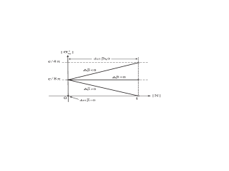
Figure 1: Variation in the spin-Hall conductivity $|\sigma^{z}_{xy}|$ with $|N|$ for three conditions $\Delta\widetilde{\beta}>0$, $\Delta\widetilde{\beta}=0$, and $\Delta\widetilde{\beta}<0$, where $Re(\lambda_{<}/\lambda_{>})$ is defined as $N$ and $|N|<1$.

When an electric field is applied in the $k_{x}$ direction, the spin-Hall response in the $k_{y}$ direction is given by

$$\sigma^{z}_{yx}=-\frac{e}{8\pi^{2}}\left(\mathrm{det}\widetilde{\beta}\right)\int_{0}^{2\pi}d\phi\frac{\sin^{2}\phi}{\Gamma(\phi)^{2}}.$$ (33)

The integration in Eq. (33) can also be calculated analytically as follows:

$$\sigma^{z}_{yx}=\left\{\begin{array}[]{cc}\displaystyle-\mathrm{sgn}(\mathrm{det}\widetilde{\beta})\frac{e}{8\pi}\left[1+\mathrm{Re}\left(\frac{\lambda_{<}}{\lambda_{>}}\right)\right]&;\mathrm{det}\widetilde{\beta}\neq 0\\ \\ 0&;\mathrm{det}\widetilde{\beta}=0\\ \end{array}\right.$$ (34)

Unlike the $\sigma^{z}_{xy}$, we have

$$\begin{split}&|\sigma^{z}_{yx}|\leq\frac{e}{8\pi},~{}\Delta\widetilde{\beta}\leq 0.\\ &\frac{e}{8\pi}<|\sigma^{z}_{xy}|<\frac{e}{4\pi},~{}\Delta\widetilde{\beta}>0.\end{split}$$ (35)

We find that when $|\sigma_{xy}^{z}|$ is larger than $e/8\pi$, $|\sigma_{yx}^{z}|$ is less than $e/8\pi$ and vice versa. In comparison with $\sigma^{z}_{xy}$ [Eq. (28)], we find that $\sigma^{z}_{xy}$ is in general not equal to $-\sigma^{z}_{yx}$ in the k-linear system.

The symmetrical result ($\sigma^{z}_{xy}=-\sigma^{z}_{yx}$) is obtained because the electric field is applied in a direction such that the asymmetric response function vanishes. Both the pure Rashba and the pure Dresselhaus systems exhibit circular energy dispersion, and the asymmetric response function always vanishes regardless of the direction of the applied electric field. In the Rashba-Dresselhaus system, if the electric field is applied along the direction of $[010]$ and the spin-Hall response occurs along $[100]$, the band splitting along the direction of the applied electric field is the same as that along the spin-Hall response direction, and thus, the asymmetric response function vanishes. However, a small change in the direction of the applied electric field would result in a non-vanishing asymmetric response function in the Rashba-Dresselhaus system. The influence of the applied electric field on the asymmetric response function is discussed in the next section.

IV Maximum value of ISHC and asymmetric response function

The direction of the applied electric field plays an important role in determining whether the system has an non-vanishing asymmetric response function. We study the asymmetric response function by rotating the coordinate system from $(k_{x},k_{y})$ to $(k_{x}^{\prime},k_{y}^{\prime})$. Consider counterclockwise rotation of the system along the along $z$ axis by an angle $\Theta$; the relationship between $(k_{x},k_{y})$ and $(k_{x}^{\prime},k_{y}^{\prime})$ is given by $k_{x}=k_{x}^{\prime}\cos\Theta-k_{y}^{\prime}\sin\Theta$ and $k_{y}=k_{x}^{\prime}\sin\Theta+k_{y}^{\prime}\cos\Theta$. The term $\beta_{i^{\prime}j^{\prime}}$ represents the matrix element of the spin-orbit matrix in the new coordinate, and they are given by $\beta_{x^{\prime}x^{\prime}}=\beta_{xx}\cos\Theta+\beta_{xy}\sin\Theta$, $\beta_{x^{\prime}y^{\prime}}=-\beta_{xx}\sin\Theta+\beta_{xy}\cos\Theta$, $\beta_{y^{\prime}x^{\prime}}=\beta_{yx}\cos\Theta+\beta_{yy}\sin\Theta$, and $\beta_{y^{\prime}y^{\prime}}=-\beta_{yx}\sin\Theta+\beta_{yy}\cos\Theta$. It can be shown that the value of $\mathrm{det}\widetilde{\beta}$ is independent of the choice of coordinates, i.e., $\mathrm{det}\widetilde{\beta}=(\beta_{xx}\beta_{yy}-\beta_{yx}\beta_{xy})=(\beta_{x^{\prime}x^{\prime}}\beta_{y^{\prime}y^{\prime}}-\beta_{y^{\prime}x^{\prime}}\beta_{x^{\prime}y^{\prime}})$. Interestingly, it can also be shown that $\sum_{ij}\beta^{2}_{i^{\prime}j^{\prime}}=\sum_{ij}\beta^{2}_{ij}$, namely, $\sum_{ij}\beta^{2}_{ij}$ is also independent of the choice of coordinates.

In the coordinate system $(k_{x}^{\prime},k_{y}^{\prime})$, the term $\sigma^{z}_{x^{\prime}y^{\prime}}$ indicates that the electric field is applied along the $k_{y}^{\prime}$ direction ($\phi^{\prime}=\pi/2$) and the corresponding spin-Hall response $J^{z}_{x^{\prime}}$ is along the $k_{x}^{\prime}$ direction ($\phi^{\prime}=0$), where the angle $\phi^{\prime}$ is measured from the positive axis of $k_{x}^{\prime}$. On the other hand, the term $\sigma^{z}_{y^{\prime}x^{\prime}}$ indicates that the electric field is applied along the $k_{x}^{\prime}$ direction ($\phi^{\prime}=0$) and the corresponding spin-Hall response $J^{z}_{y^{\prime}}$ is obtained along the $k_{y}^{\prime}$ direction ($\phi^{\prime}=\pi/2$). Therefore, in the new coordinate system, Eqs. (28) and (34) are still valid and can be written as

$$\begin{split}&\sigma^{z}_{x^{\prime}y^{\prime}}=\mathrm{sgn}(\mathrm{det}\widetilde{\beta})\frac{e}{8\pi}\left[1-\mathrm{Re}\left(\frac{\lambda^{\prime}_{<}}{\lambda^{\prime}_{>}}\right)\right],\\ &\sigma^{z}_{y^{\prime}x^{\prime}}=-\mathrm{sgn}(\mathrm{det}\widetilde{\beta})\frac{e}{8\pi}\left[1+\mathrm{Re}\left(\frac{\lambda^{\prime}_{<}}{\lambda^{\prime}_{>}}\right)\right],\end{split}$$ (36)

where

$$\mathrm{Re}\left(\frac{\lambda^{\prime}_{<}}{\lambda^{\prime}_{>}}\right)=\frac{\Gamma^{\prime}(\phi^{\prime}=0,\Theta)^{2}-\Gamma^{\prime}(\phi^{\prime}=\frac{\pi}{2},\Theta)^{2}}{\sum_{ij}\beta^{2}_{ij}+2|\mathrm{det}\widetilde{\beta}|}.$$ (37)

The energy dispersion in the new coordinate system is $\Gamma^{\prime}(\phi^{\prime},\Theta)^{2}=(\beta_{x^{\prime}x^{\prime}}^{2}+\beta_{y^{\prime}x^{\prime}}^{2})\cos^{2}\phi^{\prime}+(\beta_{x^{\prime}y^{\prime}}^{2}+\beta^{2}_{y^{\prime}y^{\prime}})\sin^{2}\phi^{\prime}+(\beta_{x^{\prime}x^{\prime}}\beta_{x^{\prime}y^{\prime}}+\beta_{y^{\prime}x^{\prime}}\beta_{y^{\prime}y^{\prime}})\sin(2\phi^{\prime})$. Equation (37) indicates that the variation in the ISHC is altered only by the difference in two band-splittings: the band-splitting along the applied electric field direction and the band-splitting along the spin-Hall response direction.

It can be shown that in the new coordinate system, $\Gamma^{\prime}(0,\Theta)$ and $\Gamma^{\prime}(\pi/2,\Theta)$ can be written as

$$\begin{split}\Gamma^{\prime}(0,\Theta)^{2}=&\Gamma(0)^{2}\cos^{2}\Theta+\Gamma(\pi/2)^{2}\sin^{2}\Theta\\ &+(\beta_{xx}\beta_{xy}+\beta_{yx}\beta_{yy})\sin(2\Theta),\\ \Gamma^{\prime}(\pi/2,\Theta)^{2}=&\Gamma(0)^{2}\sin^{2}\Theta+\Gamma(\pi/2)^{2}\cos^{2}\Theta\\ &-(\beta_{xx}\beta_{xy}+\beta_{yx}\beta_{yy})\sin(2\Theta),\end{split}$$ (38)

where $\Gamma(0)^{2}=\beta_{xx}^{2}+\beta_{yx}^{2}$ and $\Gamma(\pi/2)^{2}=\beta_{xy}^{2}+\beta_{yy}^{2}$. Therefore, in general, when $\Theta\neq 0$, $\Gamma^{\prime}(0,\Theta)$ is not equal to $\Gamma^{\prime}(\pi/2,\Theta)$, even if $\Gamma(0)=\Gamma(\pi/2)$. A small rotation of the direction of the applied electric field would lead to a non-vanishing asymmetric response function.

According to Eqs. (36) and (37), in order to enhance $\sigma^{z}_{x^{\prime}y^{\prime}}$, i.e., $|\sigma^{z}_{x^{\prime}y^{\prime}}|>e/8\pi$, the band-splitting must satisfy the condition $\Gamma^{\prime}(0,\Theta)<\Gamma^{\prime}(\pi/2,\Theta)$. This means that the electric field must be applied along the direction with the larger band-splitting in comparison with that in the direction of the spin-Hall response. On the other hand, the corresponding vaalue of $\sigma^{z}_{y^{\prime}x^{\prime}}$ is less than $e/8\pi$. Conversely, if we want to enhance $\sigma^{z}_{y^{\prime}x^{\prime}}$, i.e. $|\sigma^{z}_{y^{\prime}x^{\prime}}|>e/8\pi$, then we must have $\Gamma^{\prime}(0,\Theta)>\Gamma^{\prime}(\pi/2,\Theta)$. This means that the electric field must be applied along the direction with larger band-splitting in comparison with that in the direction of the spin-Hall response.

Therefore, we conclude that in order to obtain the ISHC $\sigma_{s}$ with $\sigma_{s}>e/8\pi$ ($\sigma_{s}$ can be $|\sigma_{x^{\prime}y^{\prime}}^{z}|$ or $|\sigma_{y^{\prime}x^{\prime}}^{z}|$), the band splitting along the direction of the applied electric field must be larger than that along the direction of the spin-Hall response.

As indicated in Sec. IV, when $\sigma_{s}>e/8\pi$, $\sigma_{s}$ still has an upper bound value of $e/4\pi$. This means that we can further enhance $\sigma_{s}$ by finding the maximum value of the asymmetric response function. In fact, it can be shown that (see Appendix B) when all the strengths of the spin-orbit interactions are fixed, the maximum value of $|\Gamma^{\prime}(0,\Theta)^{2}-\Gamma^{\prime}(\pi/2,\Theta)^{2}|$ exists for a specific direction $\Theta_{M}$ [see Eq. (55)]. This also implies that the direction of the largest band-splitting is always perpendicular to that of the smallest band-splitting on the Fermi surface. Furthermore, the existence of the maximum value $|\Gamma^{\prime}(0,\Theta)^{2}-\Gamma^{\prime}(\pi/2,\Theta)^{2}|$ on the Fermi surface provides us a method to obtain the maximum ISHC with respect to these fixed values of $\beta_{ij}$.

In the next section, we explain how the enhanced spin-Hall response is the manifestation of Berry curvature at the nearly degenerate area.

V Berry curvature and the nearly degenerate area

In this section, we analyze the Berry curvature in a system with fixed spin-orbit interactions, and for convenience, the direction of the electric field is fixed while we rotate the system (see Fig. 2).

The spin-Hall conductivity $\sigma^{z}_{xy}$ [Eq. (13)] can be written in terms of the Berry curvature as

$$\sigma_{xy}^{z}=-\frac{e}{\hbar}\frac{1}{V}\sum_{\mathbf{k}}\sum_{n=\pm}f_{\mathbf{k}n}\Omega^{(n)}_{xy}(\mathbf{k}),$$ (39)

and it can be shown that

$$\begin{split}&\Omega^{(+)}_{xy}(\mathbf{k})=+\frac{\hbar^{3}}{4m}\mathrm{det}\widetilde{\beta}\frac{\cos^{2}\phi}{k\Gamma(\phi,\Theta)^{3}},\\ &\Omega^{(-)}_{xy}(\mathbf{k})=-\frac{\hbar^{3}}{4m}\mathrm{det}\widetilde{\beta}\frac{\cos^{2}\phi}{k\Gamma(\phi,\Theta)^{3}}.\end{split}$$ (40)

The energy dispersion $\Gamma(\phi,\Theta)$ is given by $\Gamma(\phi,\Theta)^{2}=A\cos^{2}\phi+B\sin^{2}\phi+C\sin(2\phi)$, where $A=(\beta_{xx}^{2}+\beta_{yx}^{2})\cos^{2}\Theta+(\beta_{xy}^{2}+\beta_{yy}^{2})\sin^{2}\Theta+(\beta_{xx}\beta_{xy}+\beta_{yx}\beta_{yy})\sin(2\Theta)$, $B=(\beta_{xx}^{2}+\beta_{yx}^{2})\sin^{2}\Theta+(\beta_{xy}^{2}+\beta_{yy}^{2})\cos^{2}\Theta-(\beta_{xx}\beta_{xy}+\beta_{yx}\beta_{yy})\sin(2\Theta)$, and $C=(\beta_{xy}^{2}-\beta_{xx}^{2}+\beta_{yy}^{2}-\beta_{yx}^{2})\sin(2\Theta)/2+(\beta_{xx}\beta_{xy}+\beta_{yx}\beta_{yy})\cos(2\Theta)$.

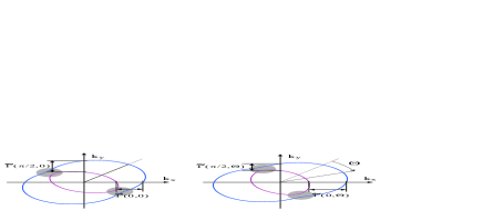
Figure 2: (Color online) Rotation of energy dispersions described by $\Theta$. The band splitting $(2m/\hbar^{2})\Gamma(\phi,\Theta)$ is defined as $(2m/\hbar^{2})\Gamma(\phi,\Theta):=\widetilde{\Gamma}(\phi,\Theta)$. The circular area (gray) represents the nearly degenerate area.

We note that the Berry curvature of outer band ($n=+1$) is opposite to that of the inner band ($n=-1$) in sign. Therefore, when both bands are occupied ($\mu>0$), the only contribution to the spin-Hall conductivity is the Berry curvature of the outer band. Namely, at a fixed value of $\phi$, the Berry curvature of the inner band cancels that of the outer band at every $k$ point with $k<k_{F}^{-}$. Equation (39) becomes

$$\sigma_{xy}^{z}=\frac{e}{\hbar}\int_{k_{F}^{-}}^{k_{F}^{+}}dS_{k}\Omega^{(+)}_{xy}(\mathbf{k}).$$ (41)

On the other hand, for $\sigma_{yx}^{z}$, we have

$$\begin{split}\sigma_{yx}^{z}=-\frac{e}{\hbar}\int_{k_{F}^{-}}^{k_{F}^{+}}dS_{k}\Omega^{(+)}_{yx}(\mathbf{k}),\end{split}$$ (42)

where

$$\Omega^{(+)}_{yx}(\mathbf{k})=+\frac{\hbar^{3}}{4m}\mathrm{det}\widetilde{\beta}\frac{\sin^{2}\phi}{k\Gamma(\phi,\Theta)^{3}}.$$ (43)

We plot the variation in the Berry curvatures $\widetilde{\Omega}_{xy}^{(+)}:=\Omega_{xy}^{(+)}/(\hbar^{3}/4m)$ and $\widetilde{\Omega}_{yx}^{(+)}:=\Omega_{yx}^{(+)}/(\hbar^{3}/4m)$ along the path $k_{F}^{+}(\phi)=m\Gamma(\phi,\Theta)/\hbar^{2}+\sqrt{(m/\hbar^{2})^{2}\Gamma(\phi,\Theta)^{2}+(2m\mu/\hbar^{2})^{2}}$. The direction of the electric field is fixed along $k_{y}$ for obtaining $\widetilde{\Omega}_{xy}^{(+)}$ or along $k_{x}$ for obtaining $\widetilde{\Omega}_{yx}^{(+)}$. The peak value of $\widetilde{\Omega}_{xy}^{(+)}$ ($\widetilde{\Omega}_{yx}^{(+)}$) is denoted as $\widetilde{\Omega}_{xy}^{(+,P)}$ ($\widetilde{\Omega}_{yx}^{(+,P)}$). The peak value refers to the value of the Berry curvature at the nearly degenerate area (see Fig. 4). The ISHCs are $|\sigma^{z}_{xy}|=(e/8\pi)(1-N)$ and $|\sigma^{z}_{yx}|=(e/8\pi)(1+N)$, where $N=[\Gamma(0,\Theta)^{2}-\Gamma(\pi/2,\Theta)^{2}]/(\sum_{ij}\beta_{ij}^{2}+2|\mathrm{det}\widetilde{\beta}|)$.

We select a system with a non-spherical energy dispersion (the nearly degenerate area exists) and $\Gamma(0,0)\neq\Gamma(\pi/2,0)$. We use the following coefficients of the spin-orbit matrix: $\beta_{xx}=6\times 10^{-2}$ eV nm, $\beta_{xy}=4.14\times 10^{-2}$ eV nm, $\beta_{yx}=4.85\times 10^{-2}$ eV nm, $\beta_{yy}=8.71\times 10^{-2}$ eV nm. The Fermi energy is 2.67 meV. The particle mass is 0.08 in units of the bare electron mass. The energy dispersion is non-spherical, as shown in the left-hand side of Fig. 4(a). The thick line represents the direction with the largest band-splitting on the Fermi surface. By using Eq. (55), we have $\Theta_{M1}\sim 0.288922\pi$ and $\Theta_{M2}\sim 0.788922\pi$. The asymmetric response function vanishes at $\Theta=\Theta_{0}$, and it can be obtained by using $\Gamma(0,\Theta_{0})=\Gamma(\pi/2,\Theta_{0})$. The result is $\Theta_{01}\sim 0.038922\pi$ and $\Theta_{02}\sim 0.538921\pi$.

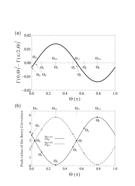
Figure 3: (a) The asymmetric response function [$\Gamma(0,\Theta)^{2}-\Gamma(\pi/2,\Theta)^{2}$ (eV cm)²] vs $\Theta$. (b) Variation of the peak values of the Berry curvatures ($\widetilde{\Omega}_{xy}^{(+,P)}$ and $\widetilde{\Omega}_{yx}^{(+,P)}$) with $\Theta$. The Berry curvatures have units of $(\hbar^{3}/4m)\times 10^{6}$. The peak values $\widetilde{\Omega}_{xy}^{(+,P)}$ ($\blacksquare$) and $\widetilde{\Omega}_{yx}^{(+,P)}$ ($\vartriangle$) correspond to Fig. 4(a) to (h).

The variations of asymmetric response function and the peak values of the Berry curvatures with $\Theta$ are shown in Fig. 3. When the system is not rotated ($\Theta=0$), the band splitting at $\phi=0$ is less than that at $\phi=\pi/2$ [Fig. 3(a)], and we have $|\sigma^{z}_{xy}|>|\sigma^{z}_{yx}|$. We find that $\widetilde{\Omega}_{xy}^{(+,P)}$ is larger than $\widetilde{\Omega}_{yx}^{(+,P)}$ as shown in Fig. 3(b).

We now rotate the system with an angle $\Theta=\Theta_{01}$ such that the band splitting at $\phi=0$ is equal to that at $\phi=\pi/2$, resulting a vanishing asymmetric response function, i.e., $\Gamma(0,\Theta_{01})=\Gamma(\pi/2,\Theta_{01})$ [Fig. 3(a)]. This results in $|\sigma^{z}_{xy}|=|\sigma_{yx}^{z}|=e/8\pi$. In Fig. 3(b), $\widetilde{\Omega}_{xy}^{(+,P)}$ is equal to $\widetilde{\Omega}_{yx}^{(+,P)}$ when $\Theta=\Theta_{01}$. If we further rotate the system such that the band splitting at $\phi=0$ is larger than that at $\phi=\pi/2$ ($\Theta_{01}<\Theta<\Theta_{M1}$), we obtain $|\sigma_{xy}^{z}|<|\sigma_{yx}^{z}|$. The corresponding $\widetilde{\Omega}_{yx}^{(+,P)}$ is now larger than $\widetilde{\Omega}_{xy}^{(+,P)}$ as can be seen in Fig. 3(b). If we rotate the system by $\Theta=\Theta_{M1}$ such that the largest band splitting is now located along the $k_{x}$ direction, the magnitude of the asymmetric response function in this case reaches a maximum value as shown in Fig. 3(a). We still have $|\sigma_{xy}^{z}|<|\sigma_{yx}^{z}|$, but $|\sigma_{yx}^{z}|$ would be very close to $e/4\pi$, and $|\sigma^{z}_{xy}|$ is less than $e/8\pi$. We find that $\widetilde{\Omega}_{yx}^{(+,P)}$ is not only considerably larger than that of $\widetilde{\Omega}_{xy}^{(+,P)}$, but is also the maximum value in comparison with the other peak values of the Berry curvatures.

When $\Theta=\Theta_{02}$, the asymmetric response function vanishes. In this case, we obtain $|\sigma_{xy}^{z}|=|\sigma_{yx}^{z}|=e/8\pi$ and $\widetilde{\Omega}_{xy}^{(+,P)}=\widetilde{\Omega}_{yx}^{(+,P)}$. When the maximum peak value of the Berry curvature $\widetilde{\Omega}_{xy}^{(+,P)}$ ($\widetilde{\Omega}_{yx}^{(+,P)}$) is obtained at $\Theta=\Theta_{M2}$ ($\Theta=\Theta_{M1}$), the magnitude of the asymmetric response function reaches a maximum value. We have $|\sigma_{xy}^{z}|>|\sigma_{yx}^{z}|$, but $\sigma_{xy}^{z}$ would be very close to $e/4\pi$, and $\sigma_{yx}$ is less than $e/8\pi$.

We select some specific angles [$\Theta_{a}\sim\Theta_{h}$ shown in Fig. 3(a) and (b)] and plot the corresponding Berry curvatures along the path $k_{F}^{+}(\phi)$ and the orientations of the energy dispersions (see Fig. 4).

As shown in Fig. 4, both the Berry curvatures ($\widetilde{\Omega}_{xy}^{(+)}$ and $\widetilde{\Omega}_{yx}^{(+)}$) have significant values (peak values) in the nearly degenerate area. When the system is rotated, both the positions of nearly degenerate area and $\widetilde{\Omega}_{xy}^{(+,P)}$ and $\widetilde{\Omega}_{yx}^{(+,P)}$ change together. Furthermore, $\widetilde{\Omega}_{yx}^{(+,P)}$ increases and $\widetilde{\Omega}_{xy}^{(+,P)}$ decreases as seen from Fig. 4(a) to (d). On the other hand, in Fig. 4(e) to (h), $\widetilde{\Omega}_{yx}^{(+,P)}$ decreases and $\widetilde{\Omega}_{xy}^{(+,P)}$ increases [see also Fig. 3(b)].

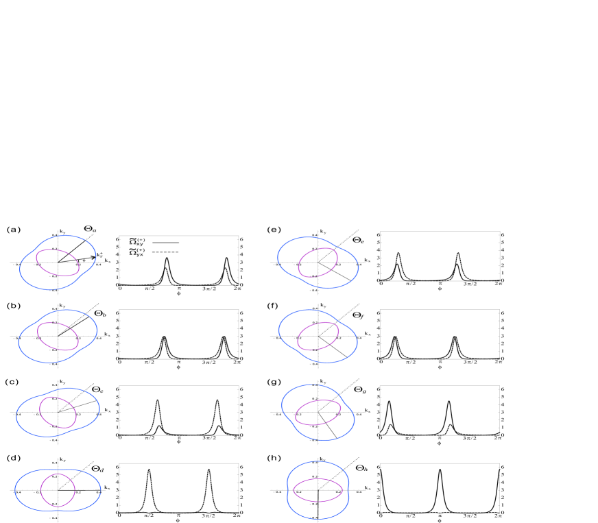
Figure 4: (Color online) Rotation of energy dispersions described by $\Theta$ and the corresponding variation in the Berry curvature $\widetilde{\Omega}_{xy}^{(+)}$ (thick line) and $\widetilde{\Omega}_{yx}^{(+)}$ (broken line) along the path $k_{F}^{+}(\phi)$, $\phi:0\sim 2\pi$. Both the Berry curvatures ($\widetilde{\Omega}_{xy}^{(+)}$ and $\widetilde{\Omega}_{yx}^{(+)}$) have units of $(\hbar^{3}/4m)\times 10^{6}$. (a)$\Theta_{a}=0$, (b)$\Theta_{b}=\Theta_{01}$, (c)$\Theta_{01}<\Theta_{c}<\Theta_{M1}$, (d)$\Theta_{d}=\Theta_{M1}$, (e)$\Theta_{M1}<\Theta_{e}<\Theta_{02}$, (f)$\Theta_{f}=\Theta_{02}$, (g)$\Theta_{02}<\Theta_{g}<\Theta_{M2}$, (h)$\Theta_{h}=\Theta_{M2}$.

The variation in the ISHCs ($|\sigma_{xy}^{z}|$ and $|\sigma_{yx}^{z}|$) corresponding to the Berry curvature variations in Fig. 4(a) to (h) is shown in Fig. 5, where $|\sigma^{z}_{xy}|=(e/8\pi)(1-N)$, $|\sigma^{z}_{yx}|=(e/8\pi)(1+N)$ and $N=[\Gamma(0,\Theta)^{2}-\Gamma(\pi/2,\Theta)^{2}]/(\sum_{ij}\beta_{ij}^{2}+2|\mathrm{det}\widetilde{\beta}|)$. The ISHC $|\sigma_{xy}^{z}|$ decreases in Fig. 5(a) to (d) and then increases in Fig. 5(e) to (h). The ISHC $|\sigma_{yx}^{z}|$ increases in Fig. 5(a) to (d) and subsequently decreases in Fig. 5(e) to (h). In the cases shown in Fig. 5(b) and (f) , $|\sigma_{xy}^{z}|=|\sigma_{yx}^{z}|$ and both the Berry curvatures have the same peak values. The behavior of the Berry curvature at the nearly degenerate area is in agreement with our conclusions in Sec. IV.

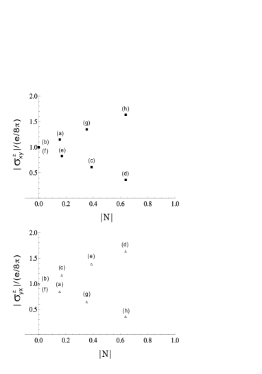
Figure 5: The numerical values of ISHCs $\sigma^{z}_{xy}$ ($\blacksquare$) and $\sigma_{yx}^{z}$ ($\vartriangle$) corresponding to different rotation angles $\Theta$ corresponding to Fig. 4(a) to (h) and $\Theta_{a}\sim\Theta_{h}$ in Fig. 3.

In the case of spherical energy dispersion (there is no nearly degenerate area), it can be shown that the Berry curvature $\widetilde{\Omega}_{xy}^{(+)}$ equivalent to $\widetilde{\Omega}_{yx}^{(+)}$ shifted by $\pi/2$. As in the non-spherical case, the Berry curvature still exhibits two significant responses along the directions of the spin-Hall current, but the shape and peak value of the Berry curvature do not change when we rotate the system. This means that $|\sigma^{z}_{xy}|=|\sigma^{z}_{yx}|$ regardless of the orientation of the system. The magnitude of the asymmetric response function always vanishes in this case, and the ISHC is a universal constant $e/8\pi$.

It must be emphasized that the angle $\Theta_{M}$ enables us to find the maximum value of the asymmetric response function for some fixed $\beta_{ij}$. If we have another set of values $\beta^{\prime}_{ij}$, the corresponding maximum value of the asymmetric response function is in general different from that with $\beta_{ij}$. The magnitude of the ISHC may further be enhanced by tuning the spin-orbit interactions to change the maximum value of the magnitude of the asymmetric response function, but it still has an upper bound of $e/4\pi$.

The measurable responses caused by the spin-Hall effect are very different from those in the present idealized system, which is infinite in size and does not include impurity scattering. Measurable quantities such as spin accumulation, however, depend on boundary conditions. The conserved spin-current considered in the present paper may correspond to smooth boundaries. Shi06 However, the presence of impurities can drastically affect clean limit results TWChen09Dis ; Kh06 ; Burkov04 ; Nomura05 . In Ref. Sherman10 , it was shown that impurity scattering does not suppress the spin-Hall conductivity in the spatially random Rahsba spin-orbit coupled system. In particular, the SU(2) formulation on extrinsic mechanism of spin Hall conductivity was recently investigated in Ref. Rai12 . However, the effects of a finite size and impurity scattering are beyond the scope of the present paper. Hopefully, our interesting predictions of higher intrinsic ISHC would stimulate measurements in 2D semiconductor systems in the near future.

VI Equilibrium spin current and spin-orbit matrix

We now turn to the discussion on equilibrium spin current in this generic k-linear spin-orbit coupled system. In Ref. Rashba03 , it was shown that even in thermodynamic equilibrium, spin current for the Rashba-Dresselhaus system does not vanish in the absence of external fields. This phenomena has arisen many discussions on the definition of spin current. Rashba04 ; Sun07 ; Shi06 ; Sab08 ; Dro11 The possibilities to detect the equilibrium spin currents have been studied in Refs. Sun07 and Sonin07 .

We calculate the equilibrium spin current by using conventional definition of spin current. In the case of the positive chemical potential ($\mu>0$), two branches are populated. In the absence of external fields, the equilibrium spin-current is the sum of the in-plane spin currents of the two branches

$$\langle J_{i}^{\sigma_{j}}\rangle=\frac{1}{V}\sum_{n\mathbf{k}}f_{\mathbf{k}n}\langle n\mathbf{k}|\frac{1}{2}\left\{\frac{\partial H}{\partial\hbar k_{i}},\frac{\hbar}{2}\sigma_{j}\right\}|n\mathbf{k}\rangle,$$ (44)

where $i,j=x,y$ and $|n\mathbf{k}\rangle$ is the eigenstate of Hamiltonian Eq. (1). From Eq. (10) and $k_{F}^{+}k_{F}^{-}=2m\mu/\hbar^{2}$, a straightforward calculation yields

$$\left(\begin{array}[]{cc}\langle J_{x}^{\sigma_{x}}\rangle&\langle J_{x}^{\sigma_{y}}\rangle\\ \langle J_{y}^{\sigma_{x}}\rangle&\langle J_{y}^{\sigma_{y}}\rangle\end{array}\right)=N_{F}\left(\begin{array}[]{cc}\beta_{yy}&-\beta_{xy}\\ -\beta_{yx}&\beta_{xx}\end{array}\right)\mathrm{det}\widetilde{\beta},$$ (45)

where $N_{F}=m^{2}/6\pi\hbar^{4}$. For specific systems, the result is in agreement with the previous results. In the pure Rashba system, where $\beta_{xy}=-\beta_{yx}=\alpha$ and $\beta_{xx}=\beta_{yy}=0$, we have $\langle J_{y}^{\sigma_{x}}\rangle=-\langle J_{x}^{\sigma_{y}}\rangle$ and $\langle J_{x}^{\sigma_{x}}\rangle=\langle J_{y}^{\sigma_{y}}\rangle=0$. In the pure Dresselhaus system, where $\beta_{xx}=-\beta_{yy}=\beta$ and $\beta_{xy}=\beta_{yx}=0$, we have $\langle J_{x}^{\sigma_{x}}\rangle=-\langle J_{y}^{\sigma_{y}}\rangle$ and $\langle J_{x}^{\sigma_{y}}\rangle=\langle J_{y}^{\sigma_{x}}\rangle=0$. It is interesting to note that the equilibrium spin current $\langle J_{i}^{\sigma_{j}}\rangle$ is related to the inverse of spin-orbit matrix $\widetilde{\beta}^{-1}$ via $\langle J_{i}^{\sigma_{j}}\rangle=N_{F}(\widetilde{\beta}^{-1})_{ij}(\mathrm{det}\widetilde{\beta})^{2}$.

We find that $\mathrm{det}\widetilde{\beta}$ also appears in the expression of equilibrium spin current Eq. (45). However, $J_{i}^{\sigma_{j}}$ occurs in the third order of $\beta_{ij}$. In this sense, Eq. (20) fails to explain the physical meaning of $\mathrm{det}\widetilde{\beta}$ in this case (see Appendix A). Recently, the equilibrium spin current in k-linear spin-orbit coupled systems is found to be link to the non-Abelian SU(2) gauge theory, where the Pauli spin matrix serves as a color index in the gauge field. Tokatly08 The resulting color current satisfies covariant conservation. The equilibrium spin current obtained from the covariant conserved color current in the Rashba-Dresselhaus systems is in agreement with Ref. Rashba03 . In the following, we apply this formalism to the generic k-linear systems.

The Hamiltonian Eq. (1) can be written in terms of SU(2) gauge field $\hbar^{2}(\mathbf{k}+\mathcal{A})^{2}/2m$, where $\mathcal{A}=\mathbf{A}_{i}\hat{e}_{i}$ and $\mathbf{A}_{i}=A_{i}^{a}\sigma_{a}$. We have

$$\begin{split}&A_{x}^{x}=\frac{m}{\hbar^{2}}\beta_{xx},~{}A_{y}^{x}=\frac{m}{\hbar^{2}}\beta_{xy}\\ &A_{x}^{y}=\frac{m}{\hbar^{2}}\beta_{yx},~{}A_{y}^{y}=\frac{m}{\hbar^{2}}\beta_{yy}.\end{split}$$ (46)

The equilibrium spin current denoted as $J_{i}^{a}$ Tokatly08 is proportional to $-i\epsilon_{abc}A^{b}_{i}F^{c}_{ij}$, where $F^{a}_{ij}\sigma_{a}=-i[\mathbf{A}_{i},\mathbf{A}_{j}]$ is the field strength.

The physical meaning of $\mathrm{det}\widetilde{\beta}$ in equilibrium spin current is now clear. The field strength in the SU(2) non-Abelian gauge field is given by Tokatly08

$$\begin{split}F^{a}_{xy}\sigma_{a}&=-i[\mathbf{A}_{x},\mathbf{A}_{y}]\\ &=-i[A_{x}^{x}\sigma_{x}+A_{x}^{y}\sigma_{y},A_{y}^{x}\sigma_{x}+A_{y}^{y}\sigma_{y}]\\ &=-i\left(A_{x}^{x}A_{y}^{y}[\sigma_{x},\sigma_{y}]+A_{x}^{y}A_{y}^{x}[\sigma_{y},\sigma_{x}]\right)\\ &=2\sigma_{z}\frac{m^{2}}{\hbar^{4}}\left(\mathrm{det}\widetilde{\beta}\right),\end{split}$$ (47)

where Eq. (46) is used. We have $F^{x}_{xy}=F^{y}_{xy}=0$ and $F^{z}_{xy}=\frac{m^{2}}{\hbar^{4}}\left(\mathrm{det}\widetilde{\beta}\right)$. That is, $\mathrm{det}\widetilde{\beta}$ plays the role of color magnetic field strength $F^{z}_{xy}$.

VII conclusions

In conclusion, we have shown that in 2D and k-linear spin-orbit coupled systems, the properties of the intrinsic spin-Hall conductivity are governed by two quantities: the effective coupling of spin and orbital motion (reflected by $\mathrm{det}\widetilde{\beta}$) and the asymmetric response function ($\Delta\widetilde{\beta}$). The effective coupling of spin and orbital motion is a discriminant for determining whether or not the spin-Hall conductivity vanishes. The decoupling of spin and orbital motion associated with band-overlapping phenomenon explains the physical origin of the sign change of the intrinsic spin-Hall conductivity.

Furthermore, the dependence of spin-orbit interaction on the spin-Hall effect and the resulting unsymmetrical properties are related to the asymmetric response function, which is determined by the difference in band-splitting along two directions: those of the applied electric field the and spin-Hall current. We varied the orientation of the system and studied the variation in the Berry curvature and the corresponding spin-Hall response. We found that maximum intrinsic spin-Hall conductivity occurs along the direction of the nearly degenerate area, which also leads to the maximization of the Berry curvature and the magnitude of the asymmetric response function. The position of the nearly degenerate area can be determined analytically. We also showed that the intrinsic spin-Hall conductivity has an upper bound value of $e/4\pi$.

In addition, we showed that the equilibrium spin current is proportional to $(\widetilde{\beta}^{-1})_{ij}(\mathrm{det}\widetilde{\beta})^{2}$, and $\mathrm{det}\widetilde{\beta}$ determines the field strength of the SU(2) non-Abelian gauge field in equilibrium spin current.

Appendix A Foldy-Wouthuysen transformation

A unitary transformation can be generally written as $U=e^{-iS}$, where the hermitian matrix $S$ can be expend in order of $\beta_{ij}$, i.e. $S=S^{(1)}+S^{(2)}+S^{(3)}+\cdots$. That is, $S^{(1)}$ represents the term proportional to the order of $\beta_{ij}$, $S^{(2)}$ the order of $\beta^{2}_{ij}$ and so on. Follow the approach of Foldy-Wouthuysen transformation, the Hamiltonian $H=\varepsilon_{\mathbf{k}}+H_{so}+V(x,y)$ under the unitary transformation $U=e^{-iS}$ is given by

$$\begin{split}H^{\prime}&=e^{iS}He^{-iS}\\ &=\varepsilon_{\mathbf{k}}+H^{(1)}+H^{(2)}+H^{(3)}+V(x,y)+o(\beta^{4}_{ij}),\end{split}$$ (48)

where

$$\begin{split}&H^{(1)}=H_{so}+[iS^{(1)},\varepsilon_{\mathbf{k}}]\\ &H^{(2)}=[iS^{(2)},\varepsilon_{\mathbf{k}}]+[iS^{(1)},H_{so}]+\frac{1}{2!}[iS^{(1)},[iS^{(1)},\epsilon_{\mathbf{k}}]]\\ \end{split}$$ (49)

and

$$\begin{split}H^{(3)}=&[iS^{(3)},\epsilon_{\mathbf{k}}]+[iS^{(2)},H_{so}]+\frac{1}{2!}[iS^{(1)},[iS^{(2)},\varepsilon_{\mathbf{k}}]]\\ &+\frac{1}{2!}[iS^{(2)},[iS^{(1)},\varepsilon_{\mathbf{k}}]]+\frac{1}{2!}[iS^{(1)},[iS^{(1)},H_{so}]]\\ &+\frac{1}{3!}[iS^{(1)},[iS^{(1)},[iS^{(1)},\varepsilon_{\mathbf{k}}]]].\end{split}$$ (50)

Because $H_{so}$ is an odd matrix, we have to find a matrix $S^{(1)}$ to cancel this term. Namely, we require $H^{(1)}=0$ and

$$H_{so}+[iS^{(1)},\varepsilon_{\mathbf{k}}]=0.$$ (51)

On the other hand, we note that $H_{so}$ is made up of the linear momentum $k_{i}$, i.e., $H_{so}=\sigma_{x}(\beta_{xx}k_{x}+\beta_{xy}k_{y})+\sigma_{y}(\beta_{yx}k_{x}+\beta_{yy}k_{y})$ and $\varepsilon_{\mathbf{k}}$ is proportional to $k^{2}$, $S^{(1)}$ is obtained by the replacements $k_{x}\rightarrow x$ and $k_{y}\rightarrow y$ in $H_{so}$. Take into account the constant $\frac{\hbar^{2}}{m}$, we have

$$iS^{(1)}=\frac{im}{\hbar^{2}}\left\{\sigma_{x}(\beta_{xx}x+\beta_{xy}y)+\sigma_{y}(\beta_{yx}x+\beta_{yy}y)\right\}.$$ (52)

Substitute Eq. (52) into $H^{(2)}$, after a straightforward calculation, we find that the last two terms $[iS^{(1)},H_{so}]+\frac{1}{2!}[iS^{(1)},[iS^{(1)},\epsilon_{\mathbf{k}}]]$ gives a diagonalized form $i\sum_{ij}\beta^{2}_{ij}+\frac{2i}{\hbar}\left(\mathrm{det}\widetilde{\beta}\right)\sigma_{z}L_{z}$. This means that $H^{(2)}$ is already diagonalized, and thus, we can choose

$$iS^{(2)}=0.$$ (53)

Substitute Eqs. (52) and (53) into $H^{(3)}$ [Eq. (50)], we obtain

$$\begin{split}H^{(3)}=&[iS^{(3)},\epsilon_{\mathbf{k}}]\\ &-\frac{2m^{2}}{3\hbar^{4}}\left(\mathrm{det}\widetilde{\beta}\right)[\{x,L_{z}\}(\sigma_{y}\beta_{xx}-\sigma_{x}\beta_{yx})\\ &+\{y,L_{z}\}(\sigma_{y}\beta_{xy}-\sigma_{x}\beta_{yy})].\end{split}$$ (54)

We find that the term in $[\cdots]$ is composed of odd matrices. Therefore, we must require $H^{(3)}=0$. In this sense, the next diagonalized part is order of $\beta^{4}_{ij}$.

Appendix B Maximum and minimum band-splitting

As shown in Sec. III and Sec. IV, the value $\Gamma^{\prime}(0,\Theta)^{2}-\Gamma^{\prime}(\pi/2,\Theta)^{2}$ determines whether the ISHC is larger than $e/8\pi$ or equal to $e/8\pi$. Furthermore, if the magnitude $|\Gamma^{\prime}(0,\Theta)^{2}-\Gamma^{\prime}(\pi/2,\Theta)^{2}|$ increases upon varying $\Theta$, the ISHC would approach a maximum value with respect to the fixed value of $\beta_{ij}$. We will show that the maximum value of $|\Gamma^{\prime}(0,\Theta)^{2}-\Gamma^{\prime}(\pi/2,\Theta)^{2}|$ exists for some angle $\Theta_{M}$ on the Fermi surface for fixed spin-orbit interactions.

First, we show that when $\Gamma^{\prime}(0,\Theta)$ reaches the maximum value for some $\Theta_{M}$, $\Gamma^{\prime}(\pi/2,\Theta)$ must reach the minimum at $\Theta_{M}$ and vice versa. From Eq. (38), the condition $(d/d\Theta)\Gamma^{\prime}(0,\Theta)^{2}=0$ at some $\Theta_{M}$ gives

$$\tan(2\Theta_{M})=\frac{2(\beta_{xx}\beta_{xy}+\beta_{yx}\beta_{yy})}{\Gamma(0)^{2}-\Gamma(\pi/2)^{2}},$$ (55)

where $\Gamma(0)=\Gamma^{\prime}(0,0)$ and $\Gamma(\pi/2)=\Gamma^{\prime}(\pi/2,0)$. It can also be shown that $(d/d\Theta)\Gamma^{\prime}(\pi/2,\Theta)|_{\Theta=\Theta_{M}}=0$. On the other hand, we redefine the parameters $A$, $B$ and $C$ as $A=\Gamma(0)^{2}$, $B=\Gamma(\pi/2)^{2}$, and $C=\beta_{xx}\beta_{xy}+\beta_{yx}\beta_{yy}$. The second derivative gives $(d/d\Theta)^{2}\Gamma^{\prime}(0,\Theta)^{2}=2(B-A)\cos(2\Theta)-4C\sin(2\Theta)$ and $(d/d\Theta)^{2}\Gamma^{\prime}(\pi/2,\Theta)^{2}=2(A-B)\cos(2\Theta)+4C\sin(2\Theta)=-(d/d\Theta)^{2}\Gamma^{\prime}(\pi/2,\Theta)^{2}$. Because the second derivative are opposite in sign for $\phi^{\prime}=0$ and $\phi^{\prime}=\pi/2$, this implies that when $\Gamma^{\prime}(0,\Theta)^{2}$ has the maximum (minimum) value, $\Gamma^{\prime}(\pi/2,\Theta)^{2}$ has the the minimum (maximum) value. In conclusion, $|\Gamma^{\prime}(0,\Theta)^{2}-\Gamma^{\prime}(\pi/2,\Theta)^{2}|$ must be the maximum value when $\Theta=\Theta_{M}$.

The energy dispersion of the $\widetilde{\beta}_{R}+\widetilde{\beta}_{1}$ system is of the form $\Gamma(\phi)^{2}=A^{2}\cos^{2}\phi+B^{2}\sin^{2}\phi$. Interestingly, it can be shown that for $\Theta=\Theta_{M}$, the energy dispersion $\Gamma(\phi,\Theta)$ in general has the same form as that of the $\widetilde{\beta}_{R}+\widetilde{\beta}_{1}$ system. Because we require $\Gamma^{\prime}(\phi^{\prime},\Theta)^{2}=(\beta_{x^{\prime}x^{\prime}}^{2}+\beta_{y^{\prime}x^{\prime}}^{2})\cos^{2}\phi^{\prime}+(\beta_{x^{\prime}y^{\prime}}^{2}+\beta_{y^{\prime}y^{\prime}}^{2})\sin^{2}\phi^{\prime}+(\beta_{x^{\prime}x^{\prime}}\beta_{x^{\prime}y^{\prime}}+\beta_{y^{\prime}x^{\prime}}\beta_{y^{\prime}y^{\prime}})\sin(2\phi^{\prime})$ to have the form $\Gamma^{\prime}(\phi^{\prime},\Theta)^{2}=A^{2}\cos^{2}\phi^{\prime}+B^{2}\sin^{2}\phi^{\prime}$, the coefficient $\beta_{x^{\prime}x^{\prime}}\beta_{x^{\prime}y^{\prime}}+\beta_{y^{\prime}x^{\prime}}\beta_{y^{\prime}y^{\prime}}$ must be zero at some $\Theta$, and it is obtained from the equation: $(\beta_{x^{\prime}x^{\prime}}\beta_{x^{\prime}y^{\prime}}+\beta_{y^{\prime}x^{\prime}}\beta_{y^{\prime}y^{\prime}})=\cos(2\Theta)(\beta_{xx}\beta_{xy}+\beta_{yy}\beta_{yx})+(\Gamma(\pi/2)^{2}-\Gamma(0)^{2})\sin(2\Theta)/2=0$. This indeed gives $\Theta=\Theta_{M}$.

Consider the Rashba-Dresselhaus system ($\widetilde{\beta}_{R}+\widetilde{\beta}_{S}$). If $k_{x}$ and $k_{y}$ lie respectively along the $[100]$ and $[010]$ directions, then $\Gamma(0)=\Gamma(\pi/2)$ and $\beta_{xx}\beta_{xy}+\beta_{yy}\beta_{yx}=2\alpha\beta\neq 0$. Equation (55) implies that $\Theta_{M}=\pi/4,3\pi/4$. (see Fig. 6) For $\Theta_{M}=\pi/4$, the resulting dispersion in the new coordinate system is given by $\Gamma^{\prime}(\phi^{\prime})^{2}=(\alpha-\beta)^{2}\cos^{2}\phi^{\prime}+(\alpha+\beta)^{2}\sin^{2}\phi^{\prime}$ and we have $\Gamma^{\prime}(0)<\Gamma^{\prime}(\pi/2)$. As a result, in order to obtain a large spin-Hall current ($\sigma_{s}>e/8\pi$), an electric field must be applied along the $k_{y}^{\prime}$ direction because the nearly degenerate area is located at $\Gamma^{\prime}(0)$. For $\Theta_{M}=3\pi/4$, we have $\Gamma^{\prime\prime}(\phi^{\prime\prime})^{2}=(\alpha+\beta)^{2}\cos^{2}\phi^{\prime\prime}+(\alpha-\beta)^{2}\sin^{2}\phi^{\prime\prime}$, and in this case, $\Gamma^{\prime\prime}(\pi/2)<\Gamma^{\prime\prime}(0)$. The electric field must be applied along the $k_{x}^{\prime\prime}$ direction for obtaining a large spin-Hall current. As shown in Fig. 6, $k_{x}^{\prime\prime}$ is obtained as the rotation of $k_{x}^{\prime}$ by $\pi/2$, and thus, it is parallel to $k_{y}^{\prime}$.

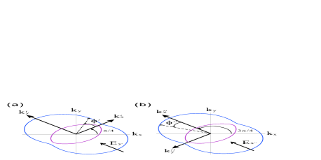
Figure 6: (Color online) The figure shows the energy dispersion in the Rashba-Dresselhaus system. The external electric field is applied along the (a) $k_{y}^{\prime}$ direction ($\Theta=\pi/4$) and (b) $k_{x}^{\prime\prime}$ direction ($\Theta=3\pi/4$).

In the Rashba-Dresselhaus system, $[110]$ and $[\bar{1}10]$ are nonequivalent axes. The corresponding band-splitting values are $2m(\alpha-\beta)/\hbar^{2}$ and $2m(\alpha+\beta)/\hbar^{2}$. We change the coordinate ($k_{x}$, $k_{y}$) to ($k_{x}^{\prime}$, $k_{y}^{\prime}$) such that $k_{x}^{\prime}$ and $k_{y}^{\prime}$ are parallel to $[110]$ and $[\bar{1}10]$, respectively. In this case, we have $\Theta_{M}=\pi/4$. The resulting effective spin-orbit matrix is

$$\frac{1}{\sqrt{2}}(\alpha-\beta)\left(\begin{array}[]{cc}1&0\\ -1&0\end{array}\right)+\frac{1}{\sqrt{2}}(\alpha+\beta)\left(\begin{array}[]{cc}0&1\\ 0&1\end{array}\right).$$ (56)

We have $\Gamma^{\prime}(0)^{2}=(\alpha-\beta)^{2}$ and $\Gamma^{\prime}(\pi/2)=(\alpha+\beta)^{2}$. The asymmetric response function $\Delta\widetilde{\beta}^{\prime}$ corresponding to the spin-orbit matrix in Eq. (56) is $\Delta\widetilde{\beta}^{\prime}=-4\alpha\beta<0$. Using Eq. (37), we can show that

$$\mathrm{Re}(\lambda^{\prime}_{<}/\lambda^{\prime}_{>})=-2\alpha\beta/[\alpha^{2}+\beta^{2}+|\alpha^{2}-\beta^{2}|].$$ (57)

For $\alpha^{2}>\beta^{2}$, the ISHCs are $\sigma^{z}_{x^{\prime}y^{\prime}}=(e/8\pi)(1+\beta/\alpha)$ and $\sigma^{z}_{y^{\prime}x^{\prime}}=-(e/8\pi)(1-\beta/\alpha)$. For $\alpha^{2}<\beta^{2}$, the ISHCs are $\sigma^{z}_{x^{\prime}y^{\prime}}=-(e/8\pi)(1+\alpha/\beta)$ and $\sigma^{z}_{y^{\prime}x^{\prime}}=(e/8\pi)(1-\alpha/\beta)$. TWChen09RDasym

Let us suppose that $\alpha>0$ and $\beta>0$, and in this case, we have $\Gamma^{\prime}(0)<\Gamma^{\prime}(\pi/2)$. The Rashba-Dresselhaus system has a smaller band-splitting of $2m(\alpha-\beta)/\hbar^{2}$ along the $[110]$ direction on the Fermi surface. On the other hand, the system has a larger band-splitting [$2m(\alpha+\beta)/\hbar^{2}$] along the $[\bar{1}10]$ direction. When the electric field is applied along the $k_{y}^{\prime}$ direction ($[\bar{1}10]$), the spin-Hall response along the $k_{x}^{\prime}$ direction indeed has a value larger than $e/8\pi$, i.e., $|\sigma^{z}_{x^{\prime}y^{\prime}}|>e/8\pi$, as shown above. Interestingly, when $\alpha$ is very close to $\beta$ in magnitude, Eq. (57) is very close to unity. The ISHC in the Rashba-Dresselhaus system would transit from $\sigma^{z}_{x^{\prime}y^{\prime}}\sim+e/4\pi$ to $\sigma^{z}_{x^{\prime}y^{\prime}}\sim-e/4\pi$ upon tuning the Rashba coupling via gate voltage.Nitta97

Rashba coupling and Dresselhaus coupling are usually of the same order of magnitude in the GaAs quantum well. Rashba05RD In the II-VI semiconductor, Rashba coupling is larger than Dresselhaus coupling, while in the III-V semiconductor, Dresselhaus coupling would be larger than Rashba coupling. Rashba05RD In the narrow-gap compounds, Rashba coupling dominates. RDmagnitude

References

- (1) G. A. Prinz, Science 282, 1660 (1998); S. A. Wolf, D. D. Awschalom, R. A. Buhrman, J. M. Daughton, S. von Molnar, M. L. Roukes, A.Y. Chtchelkanova, and D. M. Treger, Science 294, 1488 (2001).
- (2) I. Zutic, J. Fabian, and S. D. Sarma, Rev. Mod. Phys. 76, 323 (2004).
- (3) J. E. Hirsch, Phys. Rev. Lett. 83, 1834 (1999).
- (4) S. Murakami, N. Nagaosa, and S.-C. Zhang, Science 301, 1348 (2003); S. Murakami, N. Nagaosa, S.-C. Zhang, Phys. Rev. B 69, 235206 (2004).
- (5) J. Sinova, D. Culcer, Q. Niu, N. A. Sinitsyn, T. Jungwirth, and A. H. MacDonald, Phys. Rev. Lett. 92, 126603 (2004).
- (6) Y. K. Kato, R. C. Myers, A. C. Gossard, and D. D. Awschalom, Science 306, 1910 (2004).
- (7) N. P. Stern, S. Ghosh, G. Xiang, M. Zhu, N. Samarth and D. D. Awschalom, Phys. Rev. Lett. 97, 126603 (2006).
- (8) V. Sih, R. C. Myers, Y. K. Kato, W. H. Lau, A. C. Gossard, and D. D. Awschalom, Nature Physics 1, 31 (2005).
- (9) H. Engel, E. I. Rashba and B. I. Halperin, Phys. Rev. Lett. 95, 166605 (2005).
- (10) J. Wunderlich, et al, Phys. Rev. Lett. 94, 047207 (2005).
- (11) B. A. Bernevig and S.-C. Zhang, Phys. Rev. Lett. 95, 016801 (2005).
- (12) H. J. Chang, T.-W. Chen, J. W. Chen, W. C. Hong, W. C. Tsai, Y. F. Chen and G. Y. Guo, Phys. Rev. Lett. 98, 136403 (2006).
- (13) E. Saitoh, M. Ueda, H. Miyajima and G. Tatara, Appl. Phys. Lett. 88, 182509 (2006); S. O. Valenzuela and M. Tinkham, Nature (London) 442, 176 (2006); K. Ando, Y. Kajiwara, S. Takahashi, S. Maekawa, K. Takemoto, M. Takatsu and E. Saitoh, Phys. Rev. B 78, 014413 (2008).
- (14) T. Kimura, Y. Otani, T. Sato, S. Takahashi, and S. Maekawa, Phys. Rev. Lett. 98, 156601 (2007).
- (15) G. Y. Guo, S. Murakami, T.-W. Chen and Nagaosa, Phys. Rev. Lett. 100, 096401 (2008).
- (16) A. Bohm, A. Mostafazadeh, H. Koizumi, Q. Niu and J. Zwanziger, The Geometric Phase in Quantum Systems (Springer, Berlin, 2003).
- (17) T. Seki, Y. Hasegawa, S. Mitani, S. Takahashi, H. Imamura, S. Maekawa, J. Nitta and K. Takahashi, Nature Mater. 7, 125 (2008).
- (18) S.-Q. Shen, Phys. Rev. B 70, 081311(R) (2004); N. A. Sinitsyn, E. M. Hankiewicz, W. Teizer, and J. Sinova, Phys. Rev. B 70, 081312(R) (2004); M.-C. Chang, Phys. Rev. B 71, 085315 (2005); T.-W. Chen, C.-M. Huang and G. Y. Guo, Phys. Rev. B 73, 235309 (2006).
- (19) B. A. Bernevig and S.-C. Zhang, Phys. Rev. B 72, 115204 (2005); Y. Kato, R. C. Myers, A. C. Gossard, D. D. Awschalom, Nature (London) 427, 50 (2004); Y. Kato, R. C. Myers, A. C. Gossard, D. D. Awschalom, Phys. Rev. Lett. 93, 176601 (2004).
- (20) E. I. Rashba, Sov. Phys. Solid State 2, 1224 (1960); Y. A. Bychkov and E. I. Rashba, J. Phys. C 17, 6039 (1984).
- (21) G. Dresselhaus, Phys. Rev. 100, 580 (1955).
- (22) J. W. McClure, Phys. Rev. 104, 666 (1956); D. P. DiVincenzo and E. J. Mele, Phys. Rev. B 29, 1685 (1984); V. P. Gusynin and S. G. Sharapov, 95, 146801 (2005); 19.K. S. Novoselov, A. K. Geim, S. V. Morozov, D. Jiang, Y. Zhang, S. V. Dubonos, I. V. Grigorieva, and A. A. Firsov, Science 306, 666 (2004); K. S. Novoselov, A. K. Geim, S. V. Morozov, D. Jiang, M. I. Katsnelson, I. V. Grigorieva, S. V. Dubonos, and A. A. Firsov, Nature (London) 438, 197 (2005); Y. Zhang, J. P. Small, M. E. S. Amori, and P. Kim, Phys. Rev. Lett. 94, 176803 (2005); Y.-W. Tan, H. L. Stormer, and P. Kim, Nature (London) 438, 201 (2005); Y. Zhang, Y.-W. Tan, H. L. Stormer, and P. Kim, 438, 201 (2005).
- (23) N. A. Sinitsyn, A. H. MacDonald, T. Jungwirth, V. K. Dugaev and J. Sinova, Phys. Rev. B 75, 045315 (2007).
- (24) G. E. Pikus and A. N. Titkov, Optical Orientation(North-Holland, Amsterdam. 1984), p. 73.
- (25) In constructing the spin-orbit matrix , we have neglected the term which exists when . However, since is not influenced by the in-plane electric field, , we can approximately neglect this term. (see also BernePRB05 )
- (26) G. D. Mahan, Many-Particle Physics (Kluwer Academic/Plenum publisher, New York, 2000).
- (27) D. Culcer, J. Sinova, N. A. Sinitsyn, T. Jungwirth and A. H. MacDonald and Q. Niu, Phys. Rev. Lett. 93, 046602 (2004); J. Shi, P. Zhang, D. Xiao and Q. Niu, Phys. Rev. Lett. 96, 076604 (2006).
- (28) B. A. Bernevig, Phys. Rev. B 71, 073201 (2005).
- (29) L. L. Foldy and S. A. Wouthuysen, Phys. Rev. 78, 29 (1950); T.-W. Chen and D.-W. Chiou, Phys. Rev. A. 82, 012115 (2010).
- (30) M. Valin-Rodriguez, Phys. Rev. Lett. 107, 266801 (2011).
- (31) G. Arfken and H. J. Weber, Mathematical Methods for Physicists (Academic Press, 1995).
- (32) J. Sinova, S. Murakami, S.-Q. Shen and M.-S. Choi, Solid State Commun. 138, 214 (2006); J. I. Inoue, G. E. W. Bauer and L. W. Molenkamp, Phys. Rev. B 70, 041303(R) (2004); E. G. Mishchenko, A. V. Shytov and B. I. Halperin, Phys. Rev. Lett. 93, 226602 (2004); O. Chalaev and D. Loss, Phys. Rev. B 71, 245318 (2005); O. V. Dimitrova, Phys. Rev. B 71, 245327 (2005).
- (33) J. Schliemann and D. Loss, Phys. Rev. B 69, 165315 (2004); A. G. Mal’shukov and K. A. Chao, Phys. Rev. B71, 121308 (R) (2005); A. Khaetskii, Phys. Rev. B 73, 115323 (2006); N. Sugimoto, S. Onoda. S. Murakami and N. Nagaosa, Phys. Rev. B 73, 113305 (2006).
- (34) A. A. Burkov, Alvaro S. Nunez and A. H. MacDonald, Phys. Rev. B 70, 155308 (2004).
- (35) K. Nomura, J. Sinova, T. Jungwirth, Q. Niu, and A. H. MacDonald, Phys. Rev. B 71, 041304 (2005); B. K. Nikolic, L. P. Zarbo, and S. Souma, Phys. Rev. B 72, 075361 (2005); L. Sheng, D. N. Sheng, C. S. Ting, Phys. Rev. Lett. 94, 016602 (2005); E. M. Hankiewicz, L. W. Molenkamp, T. Jungwirth, and J. Sinova, Phys. Rev. B 70, 241301(R) (2004).
- (36) V. K. Duagev, M. Inglot, E. Ya. Sherman, and J. Barna, Phys. Rev. B 82, 121310(R) (2010).
- (37) R. Raimondi, P. Schwab, C. Gorini, and G. Vignale, Ann. Phys. (Berlin) 524, 153 (2012) [arXiv:1110.5279].
- (38) T.-W. Chen, H.-C. Hsu and G. Y. Guo, Phys. Rev. B 80, 165302 (2009).
- (39) E. I. Rashba, Phys. Rev. B 68, 241315(R) (2003).
- (40) E. I. Rashba, Phys. Rev. B 70, 161201(R) (2004); A. A. Burkov, A. S. Nez and A. H. MacDonald, Phys. Rev. B 70, 155308 (2004); E. B. Sonin, Phys. Rev. B 76, 033306 (2007).
- (41) Q.-f. Sun, X. C. Xie and J. Wang, Phys. Rev. Lett. 98, 196801 (2007); Phys. Rev. B 77, 035327 (2008).
- (42) V. A. Sablikov, A. A. Sukhanov and Y. Ya. Tkach, Phys. Rev. B 78, 153302 (2008).
- (43) H.-J. Drouhin, G. Fishman and J.-E. Wegrowe, Phys. Rev. B 83, 113307 (2011).
- (44) E. B. Sonin, Phys. Rev. Lett. 99, 266602 (2007).
- (45) I. V. Tokatly, Phys. Rev. Lett. 101, 106601 (2008).
- (46) J. Nitta, T. Akazaki, H. Takayanagi and T. Enoki, Phys. Rev. Lett. 78, 1335 (1997).
- (47) E. I. Rashba, Physica E: Low-dimensional Systems and Nanostructures 34, 31 (2006); Hyun C. Lee and S.-R. Eric Yang, Phys. Rev. B 72, 245338 (2005).
- (48) B. Jusserand, D. Richards, G. Allan, C. Priester and B. Etienne, Phys. Rev. B 51, 4707 (1995); W. Knap, C. Skierbiszewski, A. Zduniak, E. Litwin-Staszewska, D. Bertho, F. Kobbi, J. L. Robert, G. E. Pikus, F. G. Pikus, S. V. Iordanskii, V. Mosser, K. Zekentes, and Yu. B. Lyanda-Geller, Phys. Rev. B 53, 3912 (1996); J. B. Miller, D. M. Zumbuhl, C. M. Marcus, Y. B. Lyanda-Geller, D. Goldhaber-Gordon, K. Campman, and A. C. Gossard, Phys. Rev. Lett. 90, 076807 (2003).