Haskell_#: Coordinating Functional Processes

Francisco Heron de Carvalho-Junior
Departamento de Computação
Universidade Federal do Ceará (UFC)
Fortaleza, Brazil Rafael Dueire Lins
Centro de Informática
Universidade Federal de Pernambuco
Recife, Brazil

(June 2004)

Abstract

This paper presents Haskell_#, a coordination language targeted at the efficient implementation of parallel scientific applications on loosely coupled parallel architectures, using the functional language Haskell. Its programming environment encompasses an editor, a compiler into Petri nets, a Petri net animator and proof tool, and a skeleton library. Examples of applications, their implementation details and performance figures are presented.

1 Introduction

The peak performance of parallel architectures is growing at a faster pace than predicted by Moore’s law, that states that at each 18 months computer hardware becomes twice as fast and halves its sale price. However, parallel programming tools have not being able to reconcile portability, scalability and a higher level of abstraction without imposing severe performance penalties to applications [28].

The emerging technologies in the 1990s gave birth to new challenges in high-performance computing. The advent of clusters [8], low cost supercomputers built on top of networks of workstations and personal computers, disseminated supercomputing among academic institutions, industries and companies [11, 4, 19, 20]. More recently, advances in wide area network interconnection technologies have made possible to use their infra-structure to build distributed supercomputers of virtually infinite scale, the grids, which are particularly suitable for addressing very coarse grained scientific computing applications. Great efforts to make these technologies viable are been promoted, with promising results [34].

Clusters and grids sparkled a myriad of new applications in supercomputing for scientific computation. Most of them are not addressed adequately by contemporary tools, yielding inefficient distribution of parallel programs [83]. In [10], some parallel programming approaches used in scientific computing are compared in relation to scalability (efficiency), generality and abstraction dimensions. MPI (Message Passing Interface) [63], the most widespread message passing library, provides scalability, generality, but is less abstract than TCE (Tensor Contraction Engine) [7], PETSc [5], GA (Global Array) [66], openMP [67], auto-parallelized C/Fortran90 and HPF (High Performance Fortran) [32]. PETSc and TCE are specific purpose libraries for scientific computing, providing a high level of abstraction and scalability. Implicit approaches, such as C/Fortran90, present low scalability, high level of abstraction and high generality. These observations illustrate that, despite the efforts conducted on the last decade, the need for new parallel programming environments that reconcile a high-level of abstraction, modularity, and generality with scalability and peak performance is still a challenge [28, 77, 82].

This paper presents Haskell_#, a process-oriented coordination language [35] where Haskell [75], a language considered de facto a standard in lazy functional programming, is used for programming at computation level. Haskell_# aims to provide high-level programming mechanisms without sacrificing performance significantly, by minimizing the overheads of the management of parallelism. One of the most important concerns in Haskell_# is to make easier to prove correctness of programs. For that, a divide-and-conquer approach was adopted to increase the chances of formally analyzing programs: the process network is completely orthogonal to the sequential blocks of code (process functionality). Haskell allows sequential programs to be proved correct in a simpler fashion than their equivalent written in languages which belong to other programming paradigms. The communication primitives were designed in such a way as to allow their translation into Petri nets [72], a well reputed formalism for the specification of concurrent systems, with several analysis and verification tools [80, 12] available.

Haskell_# emphasizes compositional programming and provides support for skeletons [25]. Skeletons are used to expose topological information that can guide the Haskell_# compiler in the generation of more efficient code. MPI (Message Passing Interface) [29] is used to manage parallelism without claiming for any run-time support. Due to the recent development of inter-operable [84] and grid enabled [49] versions of MPI Haskell_# programs may be executable on grids without any extra burden.

Examples of benchmark programs and their performance figures are provided, elucidating the most important aspects of programming in Haskell_#.

This paper comprises five other sections. Section 2 gives background for programming in Haskell_#, focusing on programming abstractions. Section 3 presents motivating application examples of Haskell_# programming. Section 4 presents details about current implementation of Haskell_# for clusters. Section 5 presents performance figures about applications presented in Section 3 running on implementation described in Section 4. Section 6 concludes this paper outlining the work in progress with Haskell_#.

2 Programming in Haskell_#

Haskell_# programs are composed from a set of components, each one describing an application concern. Concerns may be functional or non-functional. Examples of functional concerns are the calculation of an exact solution for a system of linear equations and the calculation of a finite-difference approximation for a system of partial differential equations. An example of non-functional concern is the allocation of processes to processors. Components may be reused among Haskell_# programs.

In Haskell_# programming, the process of composing components is inductive. Simple components, functional modules implemented in Haskell, are basic building blocks. Given a collection of components, simple or composed ones, it is possible to define a new composed component by specifying their composition through Haskell_# Configuration Language (HCL). The result of this process is a hierarchy of components, where the main component, describing the application functionality, is at the root. Components at the leaves are simple components (always addressing functional concerns) and intermediate nodes are composed components.

Under perspective of process-oriented coordination models [35], the collection of functional modules of a Haskell_# program forms a computation medium, while the collection of composed components forms a coordination medium. The concerns on the parallel composition of Haskell functional computations are sufficiently and necessarily resolved at the coordination level. The use of Haskell for programming the computation medium allows that coordination and computation languages be really orthogonal. Lazy lists allow the overlapping of communication and computation in process execution, without to need to embed coordination extensions in the code of the functional modules.

The idea of hierarchical compositional languages implemented using configuration languages is not a recent idea [13, 1]. Haskell_# difference from its predecessor languages resides in its support for skeletons, by allowing to partially parameterize the concern addressed by components, and its ability for overlapping them, making possible to encapsulate cross-cutting concerns [21]. The use of skeletons has gained attention of parallel programming community since last decade [25] and now it is supported by many languages and paradigms [79]. The problem of modularizing cross-cutting concerns have gained attention in software engineering research community, particularly for programming large scale object-oriented systems. An example of cross-cutting concern is validation procedures executed by processes for accessing computational resources in a grid environment. With respect to this feature, Haskell_# may implement the notions of AOP (Aspect Oriented Programming) [52] and Hyperspaces [68] using an unified set of language constructors. Skeletons may be overlapped, forming more complex ones.

Haskell_# programs may be translated into Petri nets. This allows to prove formal properties and to evaluate the performance of parallel programs using automatic tools. Some previous work have addressed the problem of translating Haskell_# programs into Petri nets [56, 23]. The expressive power of HCL for describing patterns of interaction among processes is equivalent to descriptive power of labelled Petri nets [71].

Now, relevant details about how Haskell $\#$ programs are implemented are presented. HCL abstractions for programming at coordination medium are informally introduced and it is shown how simple components are programmed in Haskell. Motivating examples of Haskell_# are presented in Section 3, illustrating the use of Haskell_# programming abstractions. Appendix B formalizes an algebra for describing semantics of Haskell_# programming abstractions. The informal description points at the corresponding Haskell_# algebraic constructions.

Refer to caption — Figure 1: Process Network of MCP- $Haskell_{\#}$

2.1 Programming Composed Components

Composed components, which form coordination medium of Haskell_# programs, are programmed in HCL configurations. HCL programming corresponds to the inductive step in Haskell_# programming task described in last section. In what follows, the constructors used at coordination level for programming Haskell_# applications are informally introduced. Their formal syntax is presented in Appendix A. Appendix B brings their algebraic semantics.

01. component MCP $<$ n,m $>$ with
02.
03. iterator i range [1,n]
04.
05. use Skeletons.{PipeLine, Workpool}
06.
07. interface	IProbDef	() $\rightarrow$ (user_info, particles, tally_entries, recip, avg_e, all_tallies) where: IDispatcher () $\rightarrow$ particles
08.	behavior: seq	{	recip!; avg_e!; all_tallies!; tally_entries!; user_info!;
09.			repeat particles! until particles }
10.
11. interface	ITracking	(user_info,particles) $\rightarrow$ (events, totals) where: IPipeStage particles $\rightarrow$ events
12.	behavior: seq	{	user_info?; do process_particles; totals! }
13.
14. interface	ITallying	(tally_entries, events) $\rightarrow$ tallies where: IPipeStage events $\rightarrow$ tallies
15.	behavior: seq	{	tally_entries?; do process_events }
16.
17. interface	IStatistics	(avg_e, recip, totals, tallies) $\rightarrow$ () where: ICollector* tallies $\rightarrow$ ()
18.	behavior: seq	{	avg_e?; recip?; all_tallies?; repeat tallies? until tallies; totals? }
19.
20. unit pp; assign PipeLine $<$ 2 $>$ to pp
21. unit wp; assign WorkPool $<$ n $>$ to wp
22.
23. unit prob_def	# IProbDef wire tally_entries all2: distribute*	; assign ProbDef	to prob_def
24. unit track	# ITacking	; assign Tracking	to track
25. unit tally	# ITallying	; assign Tallying	to tally
26. unit statistics	# IStatistics	; assign Statistics	to statistics
27.
28. factorize wp.manager in $\rightarrow$ out to	dispatcher # () $\rightarrow$ out, collector # in $\rightarrow$ ()
29.
30. replace dispatcher	# tallies	$\rightarrow$ particles	by prob_def	# (_,particles,_,_,_,_)
31. replace pp.stage[1]	# particle	$\rightarrow$ events	by track	# (_, particles) $\rightarrow$ (events, _)
32. replace pp.state[2]	# events	$\rightarrow$ tallies,	by tally	# (_,events) $\rightarrow$ tallies
33. replace collector	# tallies	$\rightarrow$ (),	by statistics	# (_,_,_,tallies) $\rightarrow$ () to manager
34.
35. replicate pp into n; $[/$ replace wp.worker[i] by pp[i] $/]$
36.
37. connect prob_def $\rightarrow$ user_info	to tracking $\leftarrow$ user_info,	synchronous
38. connect prob_def $\rightarrow$ tally_entries[0]	to tallies $\leftarrow$ tally_entries,	synchronous
39. connect prob_def $\rightarrow$ tally_entries[1]	to statistics $\leftarrow$ tally_entries,	synchronous
40. connect prob_def $\rightarrow$ recip	to statistics $\leftarrow$ recip,	buffered
41. connect prob_def $\rightarrow$ avg_e	to statistics $\leftarrow$ avg_e,	buffered
42. connect tracking $\rightarrow$ totals	to statistics $\leftarrow$ totals,	buffered
43.
44. replicate m	statistics # (avg_e, recip, totals, tallies,tally_entries) $\rightarrow$ ()
45.	adjust wire	avg_e: broadcast, recip: broadcast, totals: {# (map.sum.transpose) #}
46.		tally_entries $<>$ : distribute, tallies $<>$ : broadcast

Figure 2: HCL Code for MCP-Haskell_#

MCP-Haskell_#

A parallel version of MCP-Haskell [22] is used for exemplifying the syntax of HCL. MCP-Haskell [39] is a simplified sequential version of MCNP, a code developed at Los Alamos during many years for simulating the statistical behaviour of particles (photons, neutrons, electrons, etc.) while they travel through objects of specified shapes and materials [15]. HCL code of MCP-Haskell_# is shown in Figure 2. The corresponding network topology is presented in Figure 1. The parallelism is obtained from three sources. Firstly, tracking and tallying procedures must be executed concurrently using a pipe-line. The main source of parallelism is the second. It comes from the fact that particles may be tracked and tallied independently. To take advantage of this problem feature, a work pool pattern of interaction is employed, where a manager process distributes jobs (particles) to worker processes, on demand controlled by their availability, and collects the results from each job. A third source of parallelism comes from the fact that the statistics of different tallies may be computed in parallel. Thus, each statistical process in the network is responsible for computing a specified set of tallies. In the following sections, it is explained how a HCL configuration may implement this network topology.

A HCL configuration starts with a header, declaring the name of the composed component, its static formal parameters and its arguments and return points. MCP-Haskell_# has two static parameters, $m$ and $n$ , which controls the number of parallel tasks, but no argument or return point is defined. In general, arguments and return points are not defined for the main component of an application. They are normally used in the configuration of the encapsulated functional concerns.

2.1.1 The Basic Abstractions: Units and Channels

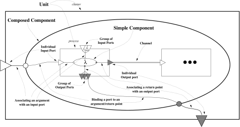
A Haskell_# configuration is specified by a collection of units, which are abstractions for agents that execute a particular task. Units synchronize using communication channels. The task performed by a unit is defined statically, by assigning a component for it. Units may be viewed as a “glue” for composing components. Units have interfaces, comprising collections of input and output ports. Interfaces are necessary for allowing units to be connected through communication channels. An interface also describes a partial order for the activation of ports during execution, characterizing the behavior of a unit. A communication channel is defined by linking two ports from opposite directions through a communication mode: synchronous, buffered and ready. Communication modes of Haskell_# channels have direct correspondence to MPI primitives, ensuring their efficient implementation, and have semantic equivalence with OCCAM [46] and CSP [43]. Ports linked through a communication channel are said to be communication pairs.

In Figure 2, lines 20 to 26 have declarations of units, whose identifiers are placed after the keyword unit. The assign declarations bind components to units. The interface of a unit is declared after the clause “#”. In the example, an interface class identifier is employed but it is possible to declare an interface directly. This topic is discussed further in the next section.

The low level of abstraction provided by units, ports and channels is not appropriate for programming large-scale and complex distributed parallel programs. Next sections introduce additional abstractions intended to raise the level of abstraction in HCL programming, simplifying the specification of large-scale and complex process topologies. Essentially, they provide support for partial topological skeletons.

2.1.2 Interface Classes

Haskell_# incorporates the notion of interface class for representing interfaces of units that present equivalent behavior. Examples of interface class declarations are shown in lines 07 to 18 of Figure 2. The identifier of an interface class is configured after the interface keyword. The notation $(i_{1},i_{2},\dots,i_{n})\rightarrow(o_{1},o_{2},\dots,o_{m})$ sets up $n$ input ports and $m$ output ports, with the respective identifiers. In a where clause, an interface composition operator (#) allows defining how an interface is obtained from the composition of existing ones. The semantics of the # operator is formalized in Appendix B.

Units that declare the same interface name after “#” clause in unit declarations inherit the same behavior, specified in the corresponding interface declaration.

A small language is embedded in behavior clause of interface declarations, intended to describe partial orders in the activation of ports. Its combinators have semantic equivalence to operators of regular expressions controlled by semaphores [47], which are regular expressions enriched with an interleaving operator, represented in HCL by the combinator par, and counter semaphores primitives, represented by the primitives wait and signal. This feature ensures that the HCL descriptive power is equivalent to the power of terminal labelled Petri nets in describing the interaction patterns between processes.

2.1.3 Wire Functions

In an assignment declaration, it is necessary to map input and output ports of the unit to arguments and return points of the assigned component, respectively. The notation $(i_{1},i_{2},\dots,i_{n})\rightarrow(o_{1},o_{2},\dots,o_{m})$ may be used whenever the order of ports does not match the order of corresponding arguments/return points.

In fact, the association between the input and output ports and the arguments and return points of components in assign declarations defines how Haskell_# glues coordination and computation media. Whenever an argument is not bound to an input port, an explicit value must be provided to it. Also, whenever a return point is not associated with an output port, it is not evaluated.

In wire clauses of unit declarations, HCL allows to define a wire function that maps a value received through an input port onto a value that is passed to an argument. Analogously, it is possible to define a wire function that receives a value produced at a return point yielding another value that is sent through the associated output port. This increases the chances that a component be reused without changing its internal implementation, in such cases where there is some type incompatibility between the type or meaning of arguments and the return points and the expected input and output ports types and meaning at coordination level.

2.1.4 Groups of Ports

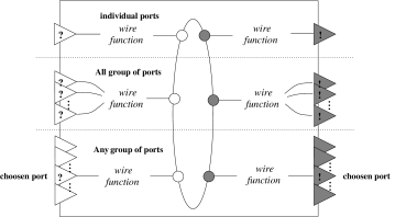
Another useful feature of HCL is the replication of interface ports of a unit, forming groups of ports where individual members are referenced using enumeration indexes. A group of ports is treated as an individual entity from the local perspective of the unit. Thus, they are bound to a unique argument/return point and must be activated atomically. However, from a global view, individual ports of the group are treated in separate, being possible to connect them through different channels.

Groups of ports may be of two kinds: any or all. When a group of input ports of kind all is activated, each port member must receive a value. The array of values received is mapped to a unique value by using a wire function. Then, the value is passed to the argument mapped onto the group of ports. When an output group of ports is activated, the value yielded at the return point mapped to it is transformed, using an wire function, into an array of values that are sent through port members of the group. In activation of groups of ports of kind any, one port belonging to the group is chosen among ports whose communication pair is activated. Once the port is chosen, communication occur like in individual ports. Notice that wire functions are necessary for configuring groups of ports of kind all. Because of that, groups of ports are configured in clause wire of unit declarations, like exemplified in Figure 2 with tally_entries group of ports. For configuring a group of ports of kind any, use any keyword instead of all keyword, as illustrated in the example. Figure 4 illustrate semantics of wire functions and groups of ports.

2.1.5 Stream Ports

Stream ports allows to transmit sequences of values (streams) terminated by an end marker. Haskell_# streams may be nested (streams of streams) at arbitrary nesting levels, which must be statically configured. Stream ports of units for which it is assigned a simple component must be mapped to argument and return points of lazy lists types in the functional module. Nested streams are associated to nested lazy lists of at least the same nesting level.

In interface declarations in lines 11 and 14, stream ports may be identified by the occurrence of sequences of symbols “*” after the identifier of the port. The number of *’s indicates its nesting level. For instance, stream ports particles and events of interface ITracking have nesting level equal to one. In Figure 9, where Haskell code of the functional module Tracking is presented, arguments and return points associated to particles and events ports of track unit are lazy lists of nesting level greater than or equal to one. Stream ports are essential for Haskell_# expressiveness, once it allows overlapping communication operations and computations during the execution of processes. The same approach is used by other parallel functional languages, such as Eden [14].

2.1.6 Configuring Arguments and Return Points of Composed Components

Arguments and return points of composed components are, respectively, input and output ports of units that are not connected through any communication channel. For speciying ports that must be connected to arguments and return points, HCL supports bind declarations.

2.1.7 The Distinction Between Processes and Clusters

It is convenient to distinguish between units associated to simple and composed components. The former are called processes, while the latter are called clusters. Processes are concrete entities and may be viewed as agents that perform sequential computations programmed in Haskell. Clusters are abstract entities and must be viewed as a parallel composition of processes. The abstraction of clusters is essential for expressing hierarchical parallelism. For example, in a constellation architecture ¹¹1Constellations have been defined as clusters of multiprocessor nodes with at least sixteen processors per node [9, 28]., a cluster must be associated with a multiprocessing node, in such a way that its comprising processes are allocated to processors for shared memory parallel execution. Instead of generating MPI code, the Haskell_# compiler could generate openMP [67] code for implementing communications among processes inside the cluster, more appropriate for multiprocessors. The support for multiple hierarchies of parallelism is essential for grid computing architectures [48] and is recognized as an important challenge for parallel programming languages designers [9].

In MCP-Haskell_# specification, pp and wp are clusters, units respectively associated to composed components PipeLine and Workpool, which represent skeletons. Units prob_def, tally, track and statistics are declared as processes. The components assigned to these units are functional modules, written in Haskell.

2.1.8 Termination of Haskell_# Programs

Units may be declared as repetitive or non-repetitive. Non-repetitive units perform a task and go to their final state, while repetitive ones always go back to their initial state, for executing its task once more. In HCL, a unit is declared repetitive by placing a symbol “*” after the keyword unit in its declaration. For declaring a cluster as repetitive, all units belonging to the composed component assigned to it must be repetitive. Otherwise, an error is detected and informed by HCL compiler.

A Haskell_# program terminates whenever all non-repetitive units belonging to its main component terminates. If it has only repetitive units, it does not terminate. Repetitive units may be used to model reactive applications.

A non-stream port of a repetitive unit may be connected to a stream port of a non-repetitive unit. Each value produced in the stream is consumed in an execution of the repetitive process.

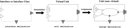
2.1.9 Virtual Units and The Support for Skeletons

A skeletons was defined above as a composed component where its addressed concern is partially defined or totally undefined. Now that the structure of composed components was scrutinized, it is possible to define Haskell_# skeletons in more precise terms. In fact, the concern addressed by a composed component is defined by the composition of concerns addressed by components assigned to its comprising units. If some unit of a component does not have a component assigned to it, it is said that the component is partially parameterized by its addressed concern. This kind of component is called a partial topological skeleton. Units not assigned to a component are called virtual units. In other skeleton-based languages, skeletons are usually total, in the sense that all units are virtual. After instantiating a partial topological skeleton, or simply a skeleton, by assigning it to a unit comprising a configuration of a component, it is possible to assign components to the virtual units of the skeleton, configuring its addressed concern.

The components Farm and Workpool are examples of total skeletons. They are used for structuring the topology of the MCP-Haskell_# program. They are instantiated by assigning them to units pp and wp, respectively. The replaces declaration, exemplified in lines 30 to 33 of Figure 2, takes a virtual unit from a skeleton and replaces it by another unit, such that there is an homomorphism relation from interface of the original unit to the interface of the new unit. This is formalized in Appendix B by the pair of relations $\sqsubseteq$ and $\sqsupseteq$ between interfaces. Indeed, replacing declarations are syntactic sugaring of HCL. The same effect could be obtained by creating a new unit, unifying it with the skeleton unit and assigning the appropriate component to the resulting unit. For that reason, replacing declarations are not formalized in Appendix B. This topic is revisited in the next section, where unification is introduced.

2.1.10 Operations over Virtual Units and Overlapping of Skeletons

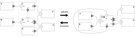
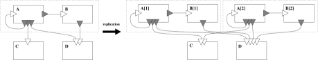
Two operations are useful for the specification of complex topologies through the composition of skeletons: unification and factorization. Unification substitutes a collection of virtual units by a new virtual unit, obeying the network connectivity and behavioral preserving restrictions formalized in the Appendix B. In this process, ports, individual or groups, may be grouped. To group groups of ports involves to merge their sets of ports. Factorization performs inverse operation of unification. It takes a unit and splits it in a collection of units, also respecting behavioral and networking connectivity preserving restrictions. It may be needed to replicate communication pairs of interface ports of a factorized unit for preserving network connectivity. Thus, it is also necessary to configure wire functions whenever a new group of ports is resulted from a factorization. For that, HCL provides clause adjust wire in unification and factorization declarations.

In Figure 6, illustrative abstract examples of unification are presented, illustrating duality between these operations. A more concrete example of factorization is presented in line 28 of Figure 2, where manager unit from Workpool skeleton is split up into units dispatcher and collector, dividing tasks realized by the manager. Unification does not appear directly in example of Figure 2. But replacing declarations, like discussed in the last section, is a syntactic sugaring of HCL that may be defined using unification. For instance, consider replacing declaration in line 31. It can be rewritten using the following equivalent code:

unit track’ # ITracking
$\vdots$
unify	pp.stage[1] # particle $\rightarrow$ events, track’ # (user_info, particles) $\rightarrow$ (events, totals)
	to track # ITracking (user_info, particles) $\rightarrow$ (events, totals)
$\vdots$
assign Tracking to track

Unification, and consequently replacing declarations, allows for overlapping skeletons. In this sense, units from distinct skeletons may be unified forming a new unit. Overlapping of skeletons is not supported by other skeleton-based languages. In general, only nesting composition has been addressed and cost models have been defined incorporating this feature [38]. A further step is to work on defining new cost models that incorporate the overlapping of skeletons.

2.1.11 Replicating Units

Another useful feature of HCL is to support replicate sub-networks from the overall network of the units described by the configuration. For that, a collection of units to be replicated and a natural number greater than one are provided. Network preserving restrictions must be observed, making necessary to replicate communication pairs of interface ports of a replicated unit, like in factorization. Wire functions must be provided to resulted groups of ports using the adjust wire clause.

Replication is exemplified in line 35 of Figure 2. The unit pp is replicated into $n$ units (pp[i], $0\leq i\leq n-1$ ), which replace worker units of Workpool skeleton. Figure 7 presents an illustrative example.

2.1.12 Indexed Notation

The # configuration language supports a special kind of syntactic sugaring for allowing to declare briefly large collections of entities. The iterator declaration employs one or more indexes and their ranging values. Syntactic elements that appear enclosed in $[/$ and $/]$ delimiters (variation scopes) are unfolded, according to range of indexes that appears on its scope. The # compiler incorporates a pre-processor for unfolding indexed notation.

In Figure 2, an iterator $i$ is declared, varying from 1 to $n$ . The replacing declaration in line 35 is put in context of a variation scope. Thus, it may be unfolded in the following code, assuming that $n=3$ :

replace wp.worker[1] by pp[1]; replace wp.worker[2] by pp[2]; replace wp.worker[3] by pp[3]

2.2 Programming Simple Components

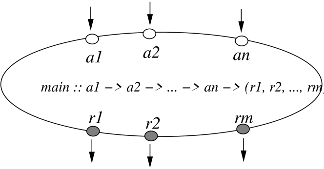
Simple components are programmed using standard Haskell. No extensions are necessary to Haskell for gluing functional modules in the coordination medium. They are connected to units at the coordination medium by assignment declarations, where a mapping between ports of the unit interface and argument/return points of the component is defined. Arguments of a functional module are represented by the collection of arguments of its function named main, while return points are represented by the elements of the returned tuple. The general signature of main is shown in Figure 8.

The main function may return values in the IO monad [90], but the I/O concerns may be resolved at coordination level using a skeleton that implements an I/O aspect, an example of cross-cutting non-functional concern.

Figure 9 presents the Haskell code for the functional module Tracking of MCP-Haskell_#. Notice the correspondence of the arguments and return points with the ports of the unit track. Functional modules are programmed in pure Haskell. There is no reference in the computation code for any element declared at the coordination level of abstraction. Other examples of functional modules, enforcing these characteristics, are provided in Figure 13.

module Tracking(main) where

import Track
import Tallies
import Mcp_types

main :: User_spec_info $\rightarrow$ [(Particle,Seed)] $\rightarrow$ ([[Event]],[Int])
main	user_info particle_list =	let	events’s = map f particle_list in (events’s, tally_bal event_lists)
	where
		f (particle@(_,_,_, e, _), sd) = (Create_source e):(track user_info particle [] sd)

Figure 9: A Functional Module from MCP-Haskell_#

2.3 Haskell_# in the Parallel Functional Languages Context

Some authors have written papers on the evolution of parallel functional languages [57, 41, 87]. It is convenient to analyze the evolution of parallel functional programming by dividing it into two periods [57]. In first one, the decades of 1970 and 1980, parallelism was viewed as possibility to make functional programs run faster. After that period, functional programming techniques have been viewed as a promising alternative to promote higher-level parallel programming, mainly motivated by the use of skeletons implemented using higher order functions [25].

The first attempts to embed the support for parallelism in functional languages suggested the technique of evaluating function arguments in parallel, with the possibility of functions absorbing unevaluated arguments and perhaps also exploiting speculative evaluation [16]. However, the granularity of the parallelism obtained from referential transparency in pure functional languages is too fine, not yielding good performance on distributed architectures. Techniques for controlling granularity, either statically or dynamically, produced little success in practice [44, 73, 50]. Implicit parallelizing compilers face difficulties to promote good load balancing amongst processors and to keep the communication costs low. On the other hand, explicit parallelism with annotations to control the demand of the evaluation of expressions, the creation/termination of processes, the sequential and parallel composition of tasks, and the mapping of these tasks onto processors yielded better results [18, 51, 45, 76, 14, 86]. GpH adopts a semi-explicit approach, where programmers may annotate the code, but responsibility to decide when to evaluate expressions in parallel is left to the compiler. Explicit approaches have the disadvantage of cross-cutting the computation and the communication code, not allowing to reason about these elements in isolation. Skeleton-based approaches have obtained a relative success in parallel functional programming [26, 42, 64, 40].

The coordination paradigm [35] influenced the design of parallel functional languages in 1990s, being exploited from two perspectives. In the first one, it is used for abstracting parallel concerns from specification of computations. Eden [14], Caliban [85], and Haskell_# focuses on these ideas. In the second one, a higher-order and non-strict style of functional programming has been seen as a convenient way for specifying the coordination amongst tasks. SCL [26] and Delirium [61] are examples of languages that employ the functional paradigm at coordination level, describing computations using languages from other paradigms. Haskell_# have other similarities with Eden and Caliban besides adopting the coordination paradigm and Haskell for describing computations. They all use constructors for explicit specification of network topologies where processes communicate through point-to-point and unidirectional channels. Like Eden, Haskell_# employs lazy lists for interleaving computation and computation and is strict in communication. Higher order values can not be transmitted through channels. Eden includes functionalities for specifying dynamic topologies, contraryse to Caliban and Haskell_#. Static parallelism is an important premise of Haskell_# design, since it is intended to analyze Haskell_# programs by translating them into Petri nets. Also, Haskell_# is oriented for high performance computing, where static parallelism is a reasonable assumption, and not for general concurrency. In the next paragraphs, some important distinguishable features Haskell_# are discussed.

The Adoption of a configuration based approach for coordination.

Configuration languages [53], integrated to a lazy functional language like Haskell, allows a complete separation between parallelism and computational programming dimensions. No extensions are required to Haskell for programming at computational level. Haskell and the HCL are orthogonal. Eden and Caliban, examples of embedded coordination languages, extend Haskell syntax with primitives for “gluing” processes to the coordination medium. GpH tries to separate parallel coordination code by using evaluation strategies [88]. Evaluation strategies is an interesting idea, but after inspecting some GpH programs that uses them, we noticed that a complete and transparent separation of the parallelism and the computation is very difficult to obtain. This is even worse when programmers want to reach peak performance of applications at any cost. The experience with Haskell_#, and other parallel functional languages, has shown that a really transparent separation makes easier to parallelize existing Haskell programs. This increases opportunities for the reuse of code and allows independent specification and development of functional modules and coordination code, reducing programming efforts and costs. The ability of composing programs from parts using the configuration approach also makes Haskell_# more suitable for programming large scale high-performance applications than other parallel functional languages [33, 27]. Programmers are forced to adopt a coarse grained view of parallelism that is convenient for clusters and grids.

The Modelling of parallel architectures.

Developing general techniques for freeing programmers from making decisions on the allocation of processes to processing nodes of a parallel architecture is an old challenge to the parallel programming community. However, this problem is hard to be treated in general. Existing mechanisms for this purpose, either dynamic or static, apply efficiently to restricted instances of the general problem and some of them are based on heuristics. With the advent of grids, cluster of heterogeneous nodes, constellations, etc, it is not expected that a unified approach, covering all realistic cases, may appear. Because of that, Haskell_# follows a static and explicit approach for process allocation, as in Caliban. Eden and GpH, on the other hand, let allocation decisions to the compiler. In Haskell_#, it is possible to model both processes needs for optimal execution and architecture characteristics by using partial topological skeletons for treating allocation as an aspect. Each skeleton may be implemented using specific allocation policies convenient for different architectures.

The analysis of formal properties using Petri nets.

The support for proving and analysing of formal properties of parallel programs by using Petri nets is one of the most important premisses that guided the design of Haskell $\#$ . A compiler that translates HCL configurations into INA [80], a Petri net analysis tool, was developed [55]. In [23], a new translation schema incorporating some extensions to the original HCL was presented. Recently, a new translation schema has appeared and we are working on a new compiler for translating Haskell_# programs into PNML [91], a format supported by many Petri net analysis tools, and SPNL [36], for analysing the performance of Haskell_# programs by using stochastic Petri nets. TimeNET [92] will be used for this purpose. Other parallel functional languages do not support formal analysis of parallel programs.

Simple and portable implementations

. Unlike other parallel functional languages, it was not necessary to modify or extend the run-time system of GHC for implementing Haskell_#. Indeed, any Haskell compiler could be used in alternative to GHC, with all optimizations enabled. Haskell_# programs take advantage of the evolution of compilation techniques with little efforts. Eden, for example, modifies GHC compiler and disables some of its optimizations [69]. Modifications to the run-time system of the Haskell compiler makes difficult to adapt the parallel language extension to new versions of the compiler. In Haskell_#, internal changes to the GHC run-time system do not require modifications to the code generated by the Haskell_# compiler. Only if the interface of some used library is changed, minor modifications are necessary. GpH and Eden developers should also carefully analyze the effects of modifications to their parallel run-time system.

Efficiency.

Potentially, Haskell_# compiler may generate efficient MPI code without using advanced compilation techniques for parallel code. This is due to the direct correspondence of HCL constructors to MPI primitives and the use of skeletons to abstract specific interaction patterns. Languages that use higher-level constructors, in the sense that parallelism is transparent or implicit, have difficulties on promoting the generation of MPI code able to take advantage of peak performance in cluster architectures and, mainly, in grid computing environments.

3 Motivating Examples

This section presents Haskell_# implementations for three applications recently used for benchmarking the parallel functional languages Eden, GpH and PMLS: Matrix Multiplication, LinSolv and Ray Tracer [59]. A Haskell_# implementation for a sub-set of NPB (NAS Parallel Benchmarks) [2] is also presented. These applications will be used in Section 5 for performance evaluation of the current Haskell_# implementation, presented in Section 4.

3.1 Matrix Multiplication

Given two square matrices $A,B\in Z^{n\times n}$ , $n\in N$ , a matrix $C\in Z^{n\times n}$ is calculated, such that $\displaystyle{C_{i,j}=\sum_{k=1}^{n}A_{i,k}*B_{k,j}}$ .

A trivial, fine-grained, parallel solution requires $n\times n$ processors. Each processor computes an element $C_{i,j}$ , from scalar product of row $i$ of $A$ and column $j$ of $B$ . This solution is obviously impractical, since large matrices are common in real applications, requiring a number of processors not supplied by contemporary parallel architectures. Three approaches are commonly used in order to aggregate computations for increasing granularity [59]:

•

Row Clustering: each process computes a set of rows of $C$ . For that, the process needs the corresponding set of rows of $A$ and all matrix $B$ ;
•

Block Clustering: each process computes a block of the resulting matrix $C$ . For that, the corresponding rows of $A$ and columns of $B$ are needed;
•

Gentleman’s algorithm: the processes are organized in a torus (circular mesh) for performing a systolic computation [78]. Each process computes a block in $C$ . At initial state, the corresponding blocks in $A$ and $B$ are arranged across processes. Then, they execute $k$ steps, where $k$ is the number of rows and columns of processes. At each step, a process sends the blocks from $A$ and $B$ that it contains to its left and down neighbors, and receive new blocks from right and top neighbors. A local computation is performed and the resulting matrix is accumulated.

{- In FILE: ManagerSkelBC_WP.hcl -}
configuration ManagerSkel a $\rightarrow$ (b,c) where

use ReadMatrix,WriteMatrix -- functional modules

unit rA	# () $\rightarrow$ (a::VMatrix)	; assign ReadMatrix to rA
unit rB	# () $\rightarrow$ (b::VMatrix)	; assign ReadMatrix to rB
unit wC	# c::Matrix $\rightarrow$ ()	; assign WriteMatrix to wC

{- In FILE: MatMultBC_WP.hcl -}
configuration MatMult $<$ N $>$ where

iterator i range [1,N]

use Skeletons.Workpool
use MatrixMult, ManagerSkel -- MatrixMult is a func. module
import MatrixMult_WF(splitM,combineM)

unit wa; assign Workpool $<$ N $>$ to wa
unit wb; assign Workpool $<$ N $>$ to wb

unify	wa.manager # c $\rightarrow$ a, wb.manager # c $\rightarrow$ b
	to manager # c $\rightarrow$ (a, b)

$[/$	un	ify	wa.worker[i] # a $\rightarrow$ c, wb.worker[i] # b $\rightarrow$ c
		to worker[i]	# (a::	VMatrix, b::VMatrix) $\rightarrow$ c::Matrix
	assign MatrixMult to worker[i] $/]$

assign ManagerSkel to manager

{- In FILE: MatMultBC_Farm.hcl -}
configuration MatMult $<$ N $>$ where

iterator i range [1,N]

use Skeletons.Farm
use ReadMatrix, MatrixMult, WriteMatrix -- functional modules
import MatrixMult_WFs(splitM,splitM_T,combineM)

unit farm_a ;
assign Farm $<$ N $,splitM,combineM>$ to farm_a
unit farm_b ;
assign Farm $<$ N $,splitM\_T,combineM>$ to farm_b

$/[$	un	ify	farm_a.worker[i] # a $\rightarrow$ c,
			farm_b.worker[i] # b $\rightarrow$ c
		to worker[i]	# (a::	VMatrix, b::VMatrix) $\rightarrow$ c::Matrix

	assign MatrixMult to worker[i]
$/]$

unify	farm_a.collector # c $\rightarrow$ (),
	farm_b.collector # c $\rightarrow$ ()
	to collector	# c::Matrix $\rightarrow$ ()

assign WriteMatrix to collector
assign ReadMatrix N $\rightarrow$ a to farm_a.distributor # () $\rightarrow$ a
assign ReadMatrix N $\rightarrow$ b to farm_b.distributor # () $\rightarrow$ b

Figure 11: Haskell_# Configuration of Block Clustering using Workpool and Farm

The above solutions differ on the number and size of messages exchanged. In Haskell_# programs, composition of skeletons may be used to describe topologies for the solutions. Firstly, consider implementations of row and block clustering using Workpool skeleton, where a manager process distributes rows or blocks, respectively, as jobs to a collection of worker processes, on demand of their availability. Once a worker finishes a job, it sends its result back to the manager and stay available for receiving another job. This technique is suitable when the number of jobs exceed the number of processors available. Load balancing is automatically achieved in architectures where processor workload or performance may vary. Because of that, it has been widely used in grid computations [34]. The unit manager in the Workpool skeleton in Haskell_# has two groups of ports of kind any: one for sending jobs to workers and another for receiving results from them. Workers receive jobs from their input ports and send results through their output ports.

{- In FILE: MatMultTorus.hcl -}
configuration MatMult $<$ N $>$ where

iterator i range [1,N*N]

use Skeletons.{Torus, Farm}
useReadMatrix, MatrixMult, WriteMatrix
import MatrixMult_WFs(splitM,combineM)

unit farm_a;	assign Farm $<$ N*N,splitM,combineM $>$ to farm_a
unit farm_b;	assign Farm $<$ N*N,splitM,combineM $>$ to farm_b
unit torus;	assign Torus $<$ N $>$ to torus

$[/$	unify	farm_a.worker[i] # a $\rightarrow$ c,
		farm_b.worker[i] # b $\rightarrow$ c,
		torus.cell[i/N][i%N] # (as_l,bs_t) $\rightarrow$ (as_r,bs_d)
		to cell[i/N][i%N]	# (	a::	Matrix, b::Matrix, as_l:: [Matrix], bs_t:: [Matrix])
				$\rightarrow$ (c::Matrix, as_r :: [Matrix], bs_d:: [Matrix]) $/]$

unify	farm_a.collector # c $\rightarrow$ (), farm_b.collector # c $\rightarrow$ () to collector	# c::Matrix $\rightarrow$ ()

assign ReadMatrix N $\rightarrow$ a to farm_a.distributor # () $\rightarrow$ a
assign ReadMatrix N $\rightarrow$ b to farm_b.distributor # () $\rightarrow$ b
$[/$ assign MatrixMult to cell[i/N][i%N] $/]$
assign WriteMatrix to collector

Figure 12: Systolic Matrix Multiplication using a Torus (HCL Code)

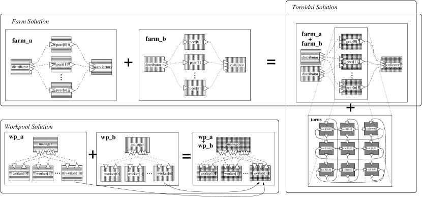
Row and block clustering may also be implemented using Farm skeleton. Now, a master process sends a job to each slave process. Ideally, jobs have similar workload. After completing a job, slaves send the result to their master and finish. The master combines the solutions received from all slaves. This approach may reduce significantly the number of messages exchanged and minimizes the communication overheads by using underlying collective communication primitives. In fact, the Farm skeleton is defined by overlapping of Gather and Scatter skeletons. Farm employs wire functions for distributing and combining values sent to and received from slave processes. For achieving better load balancing, processors must be homogeneous. This is a reasonable assumption to be made in cluster architectures, but not in grid ones.

Figure 11 presents the Haskell_# configuration codes for block clustering using Workpool and Farm skeletons. Two matrices are distributed, thus it is necessary to overlap two instances of both skeletons, as illustrated in Figure 10. The units readA, readB and writeC are clustered to implement the manager process. The implementation of row clustering makes use of identical topological description. Differences are on port types and implementation of computations. This evidences the importance of reuse and composition in Haskell_# programming.

The Gentleman’s algorithm is implemented by overlapping two instances of the Farm skeleton, one for each input matrix, with a Torus skeleton, as in Figure 10. The Torus describes the interaction pattern among slave processes from the overlapped Farms. The HCL code for this arrangement is presented in Figure 12.

module MatMult_Toroidal(main) where

import MatrixTypes

import List

main ::	Int -¿ Int -¿ Matrix -¿ Matrix -¿
	[Matrix] -¿ [Matrix] -¿ (Matrix, [Matrix], [Matrix])
main = mult’

mult’	nc nr sm1 sm2 sm1s	sm2s = (result, toRight, toDown)
	where	toRight = take (nc-1) (sm1:sm1s)
		toDown = take (nr-1) (sm2’:sm2s)
		sm2’ = transpose sm2
		sms = zipWith mult	MatricesTr
			(sm1:sm1s) (sm2’:sm2s)
		result = foldl1’ addMatrices sms

addMatrices :: Matrix -¿ Matrix -¿ Matrix
add	Matrices m1 m2 = zipWith addVectors m1 m2
	where	addVectors :: Vector -¿ Vector -¿ Vector
		addVectors v1 v2 = zipWith (+) v1 v2

multMatricesTr :: Matrix -¿ Matrix -¿ Matrix
mult	MatricesTr m1 m2 =
	[[prodEscalar row col $\mid$ col ¡- m2] $\mid$ row ¡- m1]

foldl1’ :: (a-¿a-¿a) -¿ [a] -¿ a
foldl1’ f (x:xs) = foldl’ f x xs

foldl’ :: (a -¿ b -¿ a) -¿ a -¿ [b] -¿ a
foldl’ f a [] = a
foldl’ f a (x:xs) = foldl’ f (f a x) xs

prodEscalar :: Vector -¿ Vector -¿ MyInteger
prodEscalar v1 v2 = sum (zipWith (*) v1 v2)

module LS_homSol(main) where

import Matrix
import LUDecompMatrix (det, homsolv)
import qualified Matrix (determinant)
import ModArithm

main ::	(SqMatrix Integer, Vector Integer)
	-¿ [Integer] -¿ [[Integer]]
mai	n	(a,b) = gen_xList
	where
		gen_xList :: [Integer] -¿ [[Integer]]
		gen_xList ps = map get_homSol ps

		get_homSol :: Integer -¿ [Integer]
		get_	homSol p =
			let
				b0 = vecHom p b
				a0 = matHom p a
				modDet = modHom p (determinant p a0)
				pmx = homsolv0 p a0 b0
				((iLo,jLo),(iHi,jHi)) = matBounds a
			in
				(p : modDet : if	modDet == 0
					then [0]
					else pmx)

slow_determinant :: SqMatrix Integer -¿ Integer
slow_determinant = Matrix.determinant

determinant :: Integer -¿ SqMatrix Integer -¿ Integer
determinant = det

homsolv0 ::	Integer -¿ SqMatrix Integer -¿
	Vector Integer -¿ [Integer]
homsolv0	p a0 b0 = vecCont v
	where
		v = homsolv p a0 b0

Figure 13: Functional Modules of Matrix Multiplication and LinSolv

Haskell_# components that implement the solutions above have the same names and interfaces. Only internal details, concerning the parallelism strategy adopted, varies. Thus, they can be used interchangeably in an application by nesting composition. The Haskell_# visual programming environment allows several component versions to co-exist. The programmer may choose the appropriate version, depending on the target parallel architecture. For instance, implementing matrix multiplication using Farm may be more efficient in clusters. In grids, a Workpool may prove more suitable. In supercomputers where processors are organized in a torus, the toroidal solution may be the best choice.

3.2 LinSolv

Given a matrix $A\in Z^{n\times n}$ and a vector $b\in Z^{n}$ , $n\in N$ , find an exact solution to the linear system of equations of the form $Ax=b$ .

The solution described here is exact and operates over arbitrary precision integers. A multiple homomorphic image approach is adopted [54], consisting of three stages [59]:

1.

map the input data into several homomorphic images. The domain of homomorphic images is $Z$ modulo $p$ ( $Z_{p}$ ), where $p$ is a prime number;
2.

compute the solution in each of these images, using LU-decomposition followed by forward and backward substitution;
3.

combine the results of all images into a result in the original domain, using a fold-based CRA (Chinese Remainder Algorithm) [58].

{- In FILE: ManagerLS_WP.hcl -}
configuration LS_Manager $<$ N $>$ # (ab,xList) $\rightarrow$ primes where

use LS_Input, LS_Primes, LS_CRA, LS_Output

unit input	# () $\rightarrow$ (ab,pBound,n)	; assign LS_Input	to input
unit primes	# (unlucky_primes,pBound) $\rightarrow$ (guessedNoOfPrimes,primes)	; assign LS_Primes	to primes
unit cra	# (n, guessedNoOfPrimes, xList) $\rightarrow$ (c,unlucky_primes)	; assign LS_CRA	to cra
unit output	# c $\rightarrow$ ()	; assign LS_Output	to output

connect primes $\rightarrow$ guessedNoOfPrimes	to cra $\leftarrow$ guessedNoOfPrimes
connect input_ab $\rightarrow$ n	to cra $\leftarrow$ n
connect input_ab $\rightarrow$ pBound	to primes $\leftarrow$ pBound
connect cra $\rightarrow$ unlucky_primes	to primes $\leftarrow$ unlucky_primes
connect cra $\rightarrow$ c	to output $\leftarrow$ c

{- In FILE: LinSolv_WP.hcl -}
configuration LinSolv $<$ N $>$ where

iterator i range [0,N-1]

use Skeletons.{Collective.BCast, Workpool}
use LS_Manager, LS_HomSol

unit bcast_ab	; assign BCast $<$ N $>$ to bcast_ab
unit wp	; assign Workpool $<$ N $>$ to wp

interface	ILinSolv (ab, job) $\rightarrow$ (ab,job) where: ab@IBCast # job@IWorkpool
	behavior: seq	{do ab; do job}

unify wp.manager, bcast_ab.root to ls_manager # ILinSolv
assign LS_Manager to ls_manager

$[/$	unify	wp.worker[i], bcast_ab.peer[i] to ls_worker[i] # ILinSolv
	assign HomSol to ls_worker[i] $/]$

Figure 15: LinSolv using a Workpool skeleton (HCL Code)

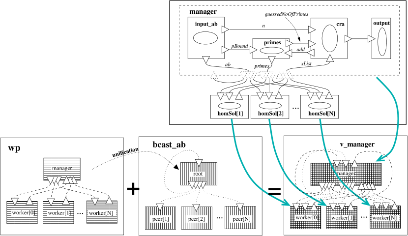
The parallel strategy implemented in Haskell_# is based on Eden and GpH versions [60]. A manager process distributes computations of homomorphic solutions as jobs to a collection of worker processes. The skeleton Workpool was adopted to distribute prime numbers to workers and to collect computed homomorphic solutions. The BCast collective communication skeleton is used for distributing working data ( $A$ and $b$ ) to the workers. The Haskell_# configuration code that implements this arrangement is presented in Figure 15. A composed component LS_Manager is configured for aggregating computations of functional modules LS_Input (obtains input data $A$ and $b$ ), LS_Primes (computes the list of primes for calculating homomorphic solutions), LS_CRA (aggregates homomorphic solutions using Chinese Remainder Algorithm), and LS_Output (outputs result $x$ ). In composed component LinSolv, the main component, a cluster is created by assigning LS_Manager to unit ls_manager, which is configured in such a way that it makes the role of root unit in BCast skeleton and manager of Workpool skeleton. The functional module LS_HomSol implements computation of a homomorphic solution for a given prime number. It is assigned to units ls_worker[i], for $0\leq i\leq N-1$ , obtained by unification of worker units of Workpool and peer units of BCast. Notice that these skeletons are overlapped. The cluster ls_manager might be placed onto a multiprocessor node, in such a way that processes input, primes, cra and output could execute concurrently. Figure 14 illustrates topological specification of LinSolv. Figure 13 shows examples of functional modules of Matrix Multiplication and LinSolv.

3.3 Ray Tracer

Given a collections of objects in the three dimensional space, calculate the corresponding two dimensional image. All rays in a window (for each pixel in the grid) are traced and their intersections with objects are computed. The colour of an intersection point is computed based on the strength of the ray and texture of the object reached [59].

{- In FILE: RT_Manager.hcl -}
configuration RT_Manager $<$ N $>$ # (rt_raytracer $\leftarrow$ xy, world) $\rightarrow$ (rt_parameters $\rightarrow$ xy[2], world) where

use RT_Parameters, RT_Result -- functional modules

unit rt_parameters	# () $\rightarrow$ (xy $<$ 2 $>$ , world) groups xy:broadcast	assign RT_Parameters to rt_paramters
unit rt_output	# (xy,res) $\rightarrow$ (); assign RT_Result to rt_output
unit rt_raytracer	# (xy,world) $\rightarrow$ res

connect rt_parameters $\rightarrow$ xy[1] to rt_output $\leftarrow$ xy

{- In FILE: RayTracer.hcl -}
configuration RayTracer $<$ N $>$ where

iterator i range [0,N-1]

use BCast, Scatter, Gather from Skeletons.Colletive
use RT_RayTracer -- functional module

unit bcast_world;	assign BCast $<$ N $>$ to bcast_world
unit scatter_xy ;	assign Scatter $<$ N $>$ to scatter_xy
unit gather_res ;	assign Gather $<$ N $>$ to gather_res

interface	IRayTracer	(xy., world., res.) $\rightarrow$ (xy., world., res.)
	where: (xy@IBCast # world@IScatter # res@IGather)
	behavior: seq	{do world; do xy; do res}

$[/$	unify	bcast_ab.peer[i], scatter_world.peer[i], gather_res.peer[i] to rt_worker[i] # IRayTracer
	assign RT_RayTracer to rt_worker[i]
$/]$

unify bcast_world.root, scatter_xy.root, gather_res.root to manager # IRayTracer
assign RT_Manager to manager
unify manager.rt_raytracer, rt_worker[0]

Figure 17: Ray Tracer (HCL Code)

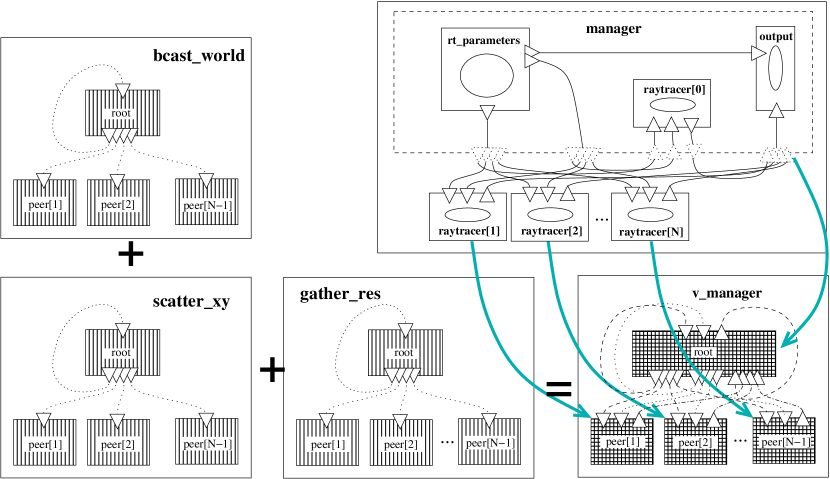
A data parallel solution is trivial, since rays can be traced independently for each pixel. In Haskell_# implementation, a direct mapping of the image lines to $N$ parallel processes, assuming one at each processor, is employed. Each process receives the same number of lines to compute. This solution yields load balancing in homogeneous clusters. The HCL for ray tracer is presented in Figure 17 and its topology is described in Figure 16. It is implemented by overlapping three skeletons: BCast, Gatherv and Scatter. The root units of these skeletons are unified to form the manager unit, responsible for distributing and collecting work among worker units, obtained by overlapping their peer units. The manager also acts as a worker. Distribution and collection are specified by wire functions. The BCast skeleton disseminates the world scene to workers. Scatter and Gatherv are used to distribute jobs and collect the results from the workers.

3.4 NAS Parallel Benchmarks

This section presents the Haskell_# implementations for a sub-set of NPB (NAS Parallel Bechmarks) [2], a package comprising eight programs, specified in NASA Research Center at Ames, USA, intended to benchmark the performance of parallel computing architectures for execution of the NAS (Numerical Aerodynamic Simulation) programs. NPB programs implemented in Haskell_# are:

•

EP (Embarrassingly Parallel) generates pairs of Gaussian deviates according to a specified scheme and tabulates the number of pairs in successive square anulli. It was developed to estimate the upper achievable limit for floating point performance in a parallel architecture;
•

IS (Integer Sorting) performs parallel sorting of $N$ keys using bucket sort algorithm. Keys are generated using a sequential algorithm described in [3] and must be uniformly distributed;
•

CG (Conjugate Gradient) implements a solution to an unstructured sparse linear system, based on conjugate gradient method. The inverse power method is used to find an estimate of the largest eigenvalue of a symmetric positive definite sparse matrix with a random pattern of non zeros;
•

LU (LU factorization) uses symmetric successive over-relaxation (SSOR) procedure to solve a block lower triangular-block upper triangular system of equations resulting from an unfactored implicit finite-difference discretization of the Navier-Stokes equations in three dimensions;

NPB programs exercise the expressiveness of HCL for describing SPMD programs and for translating MPI programs into Haskell_#. LU gave us an important insight on how to facilitate programming of applications where processes have a large number of input and output ports. CG and IS help on evaluating the performance of collective communication skeletons.

3.4.1 The Embarassingly Parallel (EP) Kernel

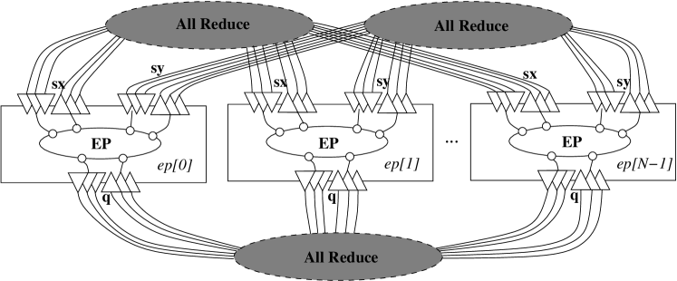
The HCL code of EP is presented in Appendix C.1. It declares $n$ units, named ep_unit[i], for $1\leq i\leq n$ . The interface class that describes the behavior of these units, IEP, is formed by the composition of three instances of IAllReduce interface class, called sx, sy and q. The definition of channels is specified by overlapping three instances of the AllReduce skeleton. For that, clusters sx_comm, sy_comm, and q_comm are associated with AllReduce component and their virtual units are unified. The HCL compiler uses the topological information provided by AllReduce skeleton and generates code that uses the MPI_AllReduce primitive of MPI.

3.4.2 The Integer Sort (IS) Kernel

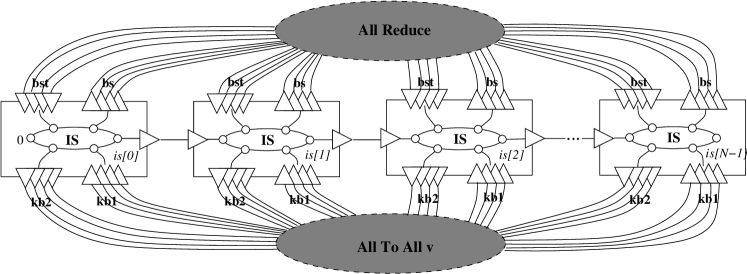
The HCL code of IS is shown in Appendix C.2. It declares a network of $n$ units, named $is\_unit[i]$ , for $1\leq i\leq n$ . The interface class for describing the behavior of IS units, called IIS, is a composition of interfaces IAllReduce, IAllToAllv and IRShif. A cyclic pattern of communication (repeat combinator) now appears, due to presence of stream ports on specification of IIS.

IS network topology is defined by overlapping skeletons AllReduce and AllToAllv, for collective communication, and RShift, which performs a data shift right amongst processes. Cluster units bs_comm, kb_comm and k_shift are assigned to them, respectively, and their virtual units are unified. The interface components $bs$ , $kb$ , $rshift$ of IIS indicate which ports of IS units participate in the skeleton instances, respectively.

3.4.3 The Conjugate Gradient (CG Kernel)

The original topology of CG, specified in FORTRAN/MPI, imposes that the number of processes, organized in a rectangular mesh, is a power of two. The version of CG in Haskell_# is less restrictive. The programmer must provide parameters $dim$ (the number of mesh rows), and $col\_factor$ (the number of mesh columns is obtained by multiplying it to $dim$ ). Any number of units may be configured using this approach, but different configurations may result in different performance. The programmer should adequate the parameters values to the features of the execution environment. CG units $cg\_unit[i][j]$ , for $1\leq i\leq dim$ and $1\leq j\leq dim*col\_factor$ . The HCL code of CG is presented in Appendix C.3.

The interface class that describes the behavior of CG units, ICG, is a composition of interface classes IAllReduce ( $rho$ , $aux$ , $rnorm$ , $norm\_temp\_1$ and $norm\_temp\_2$ ) and ITranspose ( $q$ and $r$ ). CG topology is defined by overlapping AllReduce and Transpose skeletons. The former is used for data exchange during parallel scalar products at mesh rows, and the latter for data exchange in parallel matrix multiplications, whenever a transpose operation is performed on data stored in processors. In MPI original code, several calls to MPI_Irecv primitive are needed to perform these operations, making difficult to understand the structure of the topology without a careful analysis of the parameters of the problem.

Five clusters are needed for each row of processes: $rho\_comm[i]$ , $aux\_comm[i]$ , $rnorm\_comm[i]$ , $norm\_temp\_1[i]$ , and $norm\_temp\_2[i]$ , $1\leq i\leq rows$ . The AllReduce component is assigned to them. The Transpose component is assigned to the other two clusters, $q\_comm$ and $r\_comm$ , encompassing all processes in the network. Their units are unified producing the final Haskell_# topology of CG.

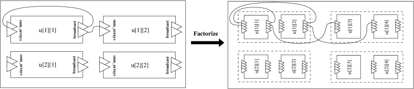
The Haskell_# configuration code of Transpose is presented in Appendix C.3.1. It organizes virtual units according to parameters $dim$ and $col\_factor$ , supplied by CG configuration. Firstly, a square mesh of units with dimension $dim$ is assembled. The ports are connected to transpose data amongst processors using appropriate wire functions applied on groups of ports. These units are factorized in $col\_factor$ units, resulting in a square mesh with $dim$ rows and $dim*col\_factor$ columns. The diagram in Figure 20 illustrates the factorization process involved in Transpose specification. In order to make it easier to understand, only channels connected to $u[1][1]$ ports are shown. They are replicated according to factorization rules.

3.4.4 The LU Factorization (LU Simulated Application)

The HCL code of LU is presented in Appendix C.4. LU organizes $n$ process, where $n$ is a power of two, in a grid. It employs the wavefront method [6] in parallel computation. It differs from other NPB programs because communication is performed by small messages of approximately 40 bytes. Another particularity of LU is the great number of communication ports in units (thirty input ports and thirty output ports). Skeletons Exchange_1b, Exchange_3b, Exchange_4, Exchange_5, and Exchange_6 describes communication topologies in several communication phases during execution, using the wavefront method. The same nomenclature employed in the original LU versions are used here to make easier to compare the two approaches. In these skeletons, there are several interfaces for virtual units that comprise them. Their specification vary according to their position in the grid. Interface generalization is useful in such cases, avoiding classes of units to be treated individually in the configuration.

4 Implementation

Haskell_# may be implemented on top of a message passing library and a sequential Haskell compiler, without any modifications or extensions to any of them. MPI 1.1 and GHC (Glasgow Haskell Compiler) are currently used, respectively. MPI is now considered the most efficient message passing library for clusters, providing standard bindings for C and Fortran. Recently, MPI versions for grid computing have appeared [49]. GHC is now considered state-of-the-art techniques for the compilation of lazy functional programs. It supports FFI (Foreign Function Interface) [24] to make direct calls to MPI routines from Haskell programs. The use of an efficient sequential Haskell compiler has important impact on performance of Haskell_# programs, since Haskell_# programs assumes medium and coarse grained parallelism, where most of time is spent in sequential mode of execution. Haskell_# implementations are easily portable to new MPI and GHC versions. Indeed, it is possible to replace GHC with any Haskell compiler that supports FFI. All optimizations and extensions provided by the Haskell compiler may be enabled. This is an important feature of Haskell_#, since other parallel functional languages built on top of GHC need to modify its run-time system. The current Haskell_# implementation has already been tested on top of LAM-MPI 6.5.9 [17], MPICH 1.2.5.2 [37] and GHC versions 6.01 and 6.2 in clusters equipped with RedHat Linux 8.0 and 9.0.

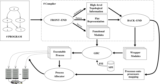
4.1 An Overview of the Haskell_# Compilation Process

The Haskell_# compiler has been entirely programmed in Haskell, using Alex 2.0 [30] and Happy 1.13 [62] for parsing. It is divided into two modules: front-end and back-end. The compilation process is illustrated in Figure 21. The front-end module parses all components of a Haskell_# program, by traversing its tree of components, from application component to simple components. A flat representation of the processes network is generated. Relevant topological information, obtained from the use of skeletons, that could guide the back-end for the generation of optimized code is stored. The flat code is currently represented as an algebraic data type in Haskell, but it is intended to implement it in XML (Extended Markup Language), allowing to use it as an intermediate language for interfacing tools for the analysis performance and formal properties in the programming environment under development.

The back-end uses flat code and topological information for generating a wrapper module for each process and for inferring the mapping of processes onto processors of the target architecture. A wrapper module is a Haskell program that controls the execution of a process. The wrapper modules and the functional modules are compiled using GHC. The mapper is a program that copies executable files onto the target machine where it will execute, based on the mapping of processes onto processors inferred by the back-end.

module Main(main) where

import System(getArgs)
import Concurrent(forkIO, Chan, newChan, newQSemN, waitQSemN, signalQSemN)
import HHashSupport
import qualified ¡Functional Module¿(main)

¡import declarations that appear in # code¿

main :: IO ()
main = do
	argv $\leftarrow$ getArgs
	argc $\leftarrow$ (return.length) argv -- MPI initialization
	give_args [] argv (mpi_init BUFFER_SIZE argc)

	$a_{1}\_chan$ :: Chan (Comm ¡Channel Type¿) $\leftarrow$ newChan --Initializing channel variables for arguments
	$a_{2}\_chan$ :: Chan (Comm ¡Channel Type¿) $\leftarrow$ newChan
	$\dots$
	$a_{n}\_chan$ :: Chan (Comm ¡Channel Type¿) $\leftarrow$ newChan

	$r_{1}\_chan$ :: Chan (Comm ¡Channel Type¿) $\leftarrow$ newChan --Initializing channel variables for return points
	$r_{2}\_chan$ :: Chan (Comm ¡Channel Type¿) $\leftarrow$ newChan
	$\dots$
	$r_{k}\_chan$ :: Chan (Comm ¡Channel Type¿) $\leftarrow$ newChan

	for	each $p$ , an individual port or group of ports involved in a collective operation:
		p $\leftarrow$	[mpi_register_port $\dots$ $\mid$ mpi_register_peer $\dots$ ]

		let comm_p = [	SingleIPort $\mid$ SingleOPort $\mid$ GroupIPort $\mid$ GroupOPort $\mid$ Bcast $\mid$ Gather $\mid$ Scatter $\mid$
			Scatterv $\mid$ Allgather $\mid$ Allgatherv $\mid$ Allreduce $\mid$ Alltoall $\mid$ Alltoallv $\mid$ Reduce_Scatter $\mid$ Scan] p $\cdots$

	caut $\leftarrow$ ¡code to setup guide automata¿
	control_automata_init caut

	sync $\leftarrow$ newQSemN 0

	forkIO (perform_actions ¿¿ signalQSemN sem)

	let	$a_{1}$ = [recv_stream $\mid$ recv_atom] [ON_DEMAND $action_{1}$ $\mid$ FORCED $chan\_a_{1}$ ]
		$a_{2}$ = [recv_stream $\mid$ recv_atom] [ON_DEMAND $action_{2}$ $\mid$ FORCED $chan\_a_{2}$ ]
		$\cdots$
		$a_{n}$ = [recv_stream $\mid$ recv_atom] [ON_DEMAND $action_{n}$ $\mid$ FORCED $chan\_a_{n}$ ]

		( $r_{1}$ , $r_{2}$ , $\dots$ , $r_{k}$ ) = ¡Functional Module¿.main $a_{1}$ $a_{2}$ $\dots$ $a_{n}$

	forkIO ([send_stream $\mid$ send_atom] $r_{1}\_chan$ $r_{1}$ ¿¿ signalQSemN sync)
	forkIO ([send_stream $\mid$ send_atom] $r_{2}\_chan$ $r_{2}$ ¿¿ signalQSemN sync)
	$\dots$
	forkIO ([send_stream $\mid$ send_atom] $r_{k}\_chan$ $r_{k}$ ¿¿ signalQSemN sync)

	waitQSemN (k+1) sem

	mpi_finalize

Figure 22: Wrapper Module

4.2 Wrapper Modules

In Figure 22, the structure of a wrapper module is illustrated. A wrapper makes a call to the main function of the functional module associated to with the process. The values produced at return points ( $r_{i}$ , $1\leq i\leq k$ ) are copied concurrently to channel variables²²2Type $Chan\ t$ from Concurrent Haskell [74]. ( $chan\_r_{j}$ ), using functions send_stream and send_atom, depending on the nature of the associated output port. The arguments provided to the main function ( $a_{j}$ , $1\leq j\leq n$ ) may also be obtained from channel variables (ON_DEMAND $chan\_r_{j}$ ) or directly (FORCED $action_{j}$ ), on demand of evaluation of return points. The function perform_actions controls the completion of the communication operations, according to a guide automaton that recognizes the behavior specified in the process interface. Whenever an output port must be activated, perform_actions evaluates perform_communication, which reads a value from the corresponding return point and sends it through the active port. For input ports, perform_communication may be called inside recv_stream or recv_atom functions, when an argument value is demanded. In this case, the operation is validated by the guide automaton and a channel variable is not necessary. However, in some collective communication operations, when a process sends and then receives a value (the root process in a broadcast, for example), it is needed to write and read, in a single call to perform_communication, channel variables associated to a return point and to an argument, respectively. This is a situation where a channel variable is necessary for an argument. The Haskell_# compiler forces evaluation of the input ports inside perform_actions whenever it may infer that an input port must be strictly activated before the activation of some output port. This is typical when the alt (choice) constructor does not occur in process behavior specification. Figure 23 illustrates the use of channel variables.

Since processes spend some time with synchronization, concurrent evaluation of perform_action and exit points, using send_stream and send_atom, allow the overlapping of computations when a process is executing perform_communication. In multiprocessors and super scalar processors, which may execute instructions in parallel and speculate about their execution, performance might be improved.

Figure 24: Guide Automaton

4.3 Guide automaton: Controlling Activation of Ports

A guide automaton is an abstract data type, implemented in C, used for controlling and validating the activation order of ports in execution of Haskell_# programs. It might be algebraically described by a tuple of the following form:

$C=(\Pi,Q,T,\varphi_{0},\varphi_{1},\rho,F,S,\sigma,\pi,\gamma,\kappa)$

where:

•

$\Pi$ is a set of port identifiers that forms the alphabet of the guide automata;
•

$Q$ is a finite set of states;
•

$T$ is a finite set of transitions;
•

$\varphi_{0}:T\rightarrow Q$ maps each transition to its origin state;
•

$\varphi_{1}:T\rightarrow Q$ maps each transition to its target state;
•

$\rho:T\rightarrow\Pi$ labels each transition with a port identifier;
•

$F\subseteq Q$ is a set of final states;
•

$S$ is a finite set of symbols, representing semaphores;
•

$\sigma:Q\rightarrow 2^{S\times Nat}$ associates states to semaphore updates. For instance, consider a semaphore $s\in S$ . If $(s,n)\in\sigma(q)$ then the value of $s$ must be incremented by $n$ when entering state $q$ ;
•

$\pi:Q\rightarrow\{forward,choice,fork,join\}$ gives the kinds of the states;
•

$\gamma:Q\rightarrow\{True,False\}$ maps choice states to an expression (termination condition of a repeat combinator) that evaluates to True or False;
•

$\kappa:Q\rightarrow 2^{Q}\times 2^{Q}$ associates a state $q$ , to a pair of set of states $(Q^{l},Q^{r})$ , whose meaning depends on $\pi(q)$ (see the next paragraph).

States and transitions are represented as natural numbers. The initial state is 0 (zero). Let $q$ be the current state of a guide automaton. The function perform_actions looks up $\kappa(q)$ in order to choose the next communication operation to be performed. For instance, consider $\kappa(q)=(Q^{l},Q^{r})$ . There must be a path from state $q$ to each state in $Q^{l}\cup Q^{r}$ . If $\pi(q)=forward$ , $Q^{r}=\emptyset$ and $Q^{l}$ determines the forward states of $q$ . Among them, the goal states are chosen. For that, let us consider a set of transitions $T^{r}=\{t\mid\varphi_{1}(t)=q^{\prime}\wedge q^{\prime}\in Q^{l}\wedge\mbox{t is in a path from $q$ to $q^{\prime}$}\}$ . Port $p$ is chosen from ports $\{p\mid t\in T^{r}\wedge\rho(t)=p\}$ , among those whose communication pairs are active at that instant (ready for communication). Forward states $\overline{q}$ , such that, for some $t\in T^{r}$ , $\varphi_{1}(t)=\overline{q}$ and $\rho(t)=p$ , are goal states. Choices appear only in the implementation of occurrences of the alt constructor. The port $p$ is activated. If $p$ is an output port (default case), it may cause the implicit activation of input ports, in recv_stream or recv_atom function calls, before completing communication. After any port activation in perform_communication, the advance_automata function is called for updating the current automata state, validating the operation, by raising an error whenever there is no transition from the current state labelled with the activated port, and updated semaphores. After the activation of $p$ , the guide automaton must be in one of the goal states. Otherwise, the operation is invalid. If $\pi(q)=choice$ , $\gamma(q)$ must be evaluated (termination condition of a repetition). If $\gamma(q)$ is true, the set of forward states of $q$ is $Q^{l}$ , otherwise it is $Q^{r}$ . Choice states are used in the implementation of occurrences of repeat and if combinators. If $\pi(q)=fork$ , $Q^{r}=\emptyset$ and $\forall t:\varphi_{0}(t)=q:\varphi_{1}(t)\in Q^{l}\wedge\rho(t)=\bot$ . When a fork state is reached, threads are forked for executing communication actions starting from the states in $Q^{l}$ . All threads must reach the same join state, where they finalize and resume execution from that state. If $\pi(q)=join$ , $Q^{l}=\emptyset$ and $Q^{r}=\emptyset$ . Fork and join states are used to implement occurrences of par combinator. If there is no forward state from current state and it is a final state, perform_actions finalizes.

Semaphores are updated in calls to advance_automata. The function $\sigma$ is used to update their values according to the new current state. A semaphore must have more than one value at a time. During execution, it must be guaranteed that all semaphores must be at least one positive value. Otherwise, an error is informed. Negative values are discarded. Semaphores only exist for validating non-regular patterns of communication that may be described by labelled Petri nets [89]. However, in general, regular patterns of communication are sufficient to describe behavior of most of high-performance parallel programs [65, 70]. Thus, overhead due to semaphore updating might be avoided for parallel programs where peak performance is critical.

4.4 Implementing Communication Operations

There are two kinds of communication operations in Haskell_#: point-to-point and collective. The former is implemented through simultaneous activation of channel’s communication pairs. MPI tags, in message envelopes, represent communication channels in calls to point-to-point primitives. The later is implemented using MPI support for dynamic configuration of communication groups and contexts and MPI collective communication primitives. Groups of ports involved in a collective communication are called communication peers. Each communication pair is configured using the function mpi_register_pair, while communication peers are configured in a single call to mpi_register_peers. These functions are implemented in C, being called from Haskell code through FFI. Their arguments, detailed in Table 1, set up parameters for completion of communication operations over involved ports during execution. A communication handle, an integer number, is returned and bound to a variable for allowing to access pair/peers information whenever necessary.

Table 1: Meaning of parameters of mpi_register_pair and mpi_register_peers

Parameter	pair	peer	Description
Direction	$\star$		Specifies if a port is for input or output
Source/Target rank	$\star$		Rank of the process that owns its comm. pair
Channel tag	$\star$		A number that identifies individually a channel
Collective Op. Type		$\star$	Kind of the collective communication operation
Number of Processes		$\star$	Number of processes in the collective operation
Processes in group		$\star$	Ranks of processes in the collective operation
Buffer Size	$\star$	$\star$	Buffer used for storing data to be transmitted
Data Type		$\star$	MPI data type (used in a reduce operations)
Reduce Operation		$\star$	MPI operation (used in a reduce operations)
Is Probed Flag	$\star$		Flag indicating if a port belongs to a choice group
Pair is Probed Flag	$\star$		Flag indicating if the communication pair of a
			port belongs to a choice group.

The polymorphic and higher-order function perform_communication has one argument, a value from the algebraic data type PortInfo t u v, whose constructors identifies the kind of communication operation to be performed: SingleIPort, SingleOPort, GroupIPort, GroupOPort (point-to-point communication), Bcast, Gather, Scatter, Scatterv, Allgather, Allgatherv, Allreduce, Alltoall, Alltoallv, Reduce_Scatter, Scan (collective communication. The PortInfo’s fields encapsulate necessary information for completion of communication operations: communication handle, port type (choice or combine), wire functions, and channel variables. The type variables $t$ , $u$ and $v$ are used for generalization of channel variables and wire functions types.

The MPI point-to-point communication primitive used for completion of communication over an output individual port (SingleOPort) depends on the communication mode of the channel where it is linked: buffered (MPI_Bsend), synchronous (MPI_Ssend) or ready (MPI_Rsend). For groups of output ports of kind All, the corresponding asynchronous MPI sending primitives (MPI_Ibsend, MPI_Issend and MPI_Irsend) are used for initiating the communication on each port belonging to the group. Then, a call to MPI_Waitall waits for the completion of all the returned request. Similarly, a call to MPI_Recv implements the communication on individual input ports, while MPI_Irecv (asynchronous) and MPI_Waitall, implements groups of input ports of kind All. Groups of ports of kind Any are implemented using the channel probing protocol, which allows the verification of the status of activation of communication pairs.

Transmitting streams and atom values.

In Haskell_#, a value of type $t$ is transmitted as a value of algebraic type Comm $t$ , whose Haskell representation is depicted below:

data Comm $t$ = Atom {data :: $t$ } $\mid$ Mid {data :: $t$ } $\mid$ End {depth::Int}

The Atom constructor encapsulates atomically transmitted values, while streamed ones are encapsulated using Mid and End constructors. The integer value in the End field represents the depth of a finalized stream. For instance, consider a stream port $p$ of type (Int,Int) and nesting factor 2 (p**::(Int,Int)). The lazy list associated to the port must be of type [[(Int,Int)]]. Consider the lazy list [[[(1,2),(3,4)], [(5,6)]], [[(7,8),(9,0),(1,2)]], [[], [(3,4)], [(5,6),(7,8)]]]. The list of values effectively transmitted through the stream port $p$ at each activation is [Mid (1,2),Mid (3,4), End 3, Mid (5,6), End 3, End 2, Mid (7,8), Mid (9,0),Mid (1,2), End 3, End 2, End 3, Mid (3,4), End 3, Mid (5,6), Mid (7,8), End 3, End 2, End 1]. Whenever possible, stream communication is implemented using MPI persistent communication objects, for minimizing communication overhead.

Marshalling Haskell Values to C Buffers.

In order to transmit Haskell values using MPI primitives, they must be marshalled onto $C$ contiguous buffers. For that, the Storable class, from FFI, is employed. Default Storable instances are provided for basic data types. User defined data types should be instantiated for this class. The Haskell_# compiler traverses Haskell modules of the Haskell_# program for finding user defined type values that must be instantiated for the Storable class. Structured data types, such as lists, arrays, tuples and algebraic data types must be packed and unpacked element by element. This could result in a considerable source of inefficiency when number of elements is very large. The benchmarks presented in Section 5.1 evidence this fact. GHC provides unboxed arrays, whose values are stored in contiguous memory areas and can be directly marshalled to MPI buffers. Since most high performance computing applications operate over arrays, and not using lists, unboxed arrays may be used in order to avoid this source of inefficiency.

5 Performance Evaluation

This section presents some performance figures for Haskell_# programs presented in Section 3. The architecture used is a Beowulf cluster comprising 16 dual Intel Xeon processors (clock: 2 GHz, RAM: 1GB), connected through a Fast Ethernet (100MBs). Measures with 32 nodes were performed in dual multiprocessing mode. MPICH 1.2.3 on top of TCP/IP was used for communication between processes.

5.1 Benchmarking Haskell_# with NPB

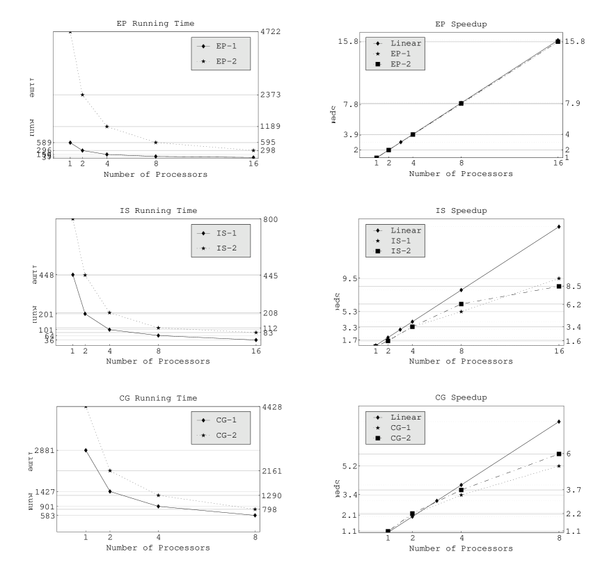
The benchmark results of Haskell_# versions of NPB kernels (EP, IS and CG) are presented in Figure 25. The plots to left hand side present their respective running times, while the plots at right hand side presents their corresponding absolute speedups, comparing them to linear speedup, always represented by a solid line.

Two problem instances were used for measuring performance of Haskell_# kernel versions (Table 2). In the second one, processes demand about twice as much memory space as the first one, without exhausting physical memory resources of a single node of the cluster. The default problem classes of NPB (S,W,A,B,C) were not used because they were tuned for use with C/FORTRAN + MPI original versions. Due to laziness and the use of immutable arrays, sequential performance of Haskell_# versions are about an order of magnitude worse than the performance of the original versions of NPB kernels, both considering time and space. Because of that, some default problem sizes exhaust physical memory resources of cluster nodes, causing virtual memory overheads that must be avoided in measures. The use of mutable arrays could minimize this source of inefficiency, but they require the encapsulation of computations inside the IO monad, preventing arrays of being transmitted through lazy lists.

Table 2: Instances of Problem Sizes Used to Run Each Kernel

Kernel	$1^{st}$ Problem Size	$2^{nd}$ Problem Size
EP	$m$ = 25	$m$ = 28
IS	$total\_keys\_log2$ = 20	$total\_keys\_log2$ = 21
	$max\_key\_log2$ =16	$max\_key\_log2$ =17
CG	$na$ = 14000	$na$ = 18000
	$nonzer$ = 11	$nonzer$ = 12
	$niter$ = 45	$niter$ = 45

Also due to performance differences in sequential mode of execution, granularity of Haskell_# processes is coarser than the granularity of processes in original NPB versions. While Haskell computations execute slower than C/FORTRAN computations, the amount of data transmitted is about the same. The original speedup measures of NPB kernels serve only to establish the lower bounds of the performance of the cluster. One should not use that to make assumptions and claims about relative efficiency of Haskell_# implementation.

Table 3: Cost Centre Analysis of IS and CG (% of total execution time)

		i	ii	iii	iv	v		i	ii	iii	iv	v
SEQ		45,9	-	-	-	54,1		90,2	-	-	-	9,8
2		35,4	3,0	7,4	4,6	45,3		79,1	1,5	2,1	4,7	7,7
4	IS-1	37,6	3,0	7,2	11,0	35,7	CG-1	70,9	1,8	3,2	11,6	5,8
8		36,0	2,7	7,2	20,8	28,7		57,5	3,5	5,6	24,0	2,7
16		34,0	2,5	7,1	27,8	24,4		50,5	4,1	7,3	32,7	1,9
SEQ		34,5	-	-	-	65,5		84,5	-	-	-	15,5
2		38,6	2,8	6,7	5,4	49,3		68,5	1,2	1,7	10,8	11,6
4	IS-2	35,3	2,8	6,8	11,7	38,9	CG-2	70,2	1,5	2,5	12,9	6,3
8		32,8	2,7	7,0	21,1	32,6		61,1	3,2	5,1	19,5	4,5
16		30,1	2,7	7,2	27,8	28,7		58,5	3,5	5,6	25,0	2,7

i: Raw computation time, ii: Evaluation of wire functions, iii: Marshalling,
iv: Communication and synchronization, v: Garbage Collection

Using GHC profiling tools [81], five main cost centres were identified in CG and IS Haskell_# implementations. Table 3 presents the impact of each of them in parallel execution. The impact of cost centres in speedup is evaluated on Table 4. By analyzing the data obtained, one may be conclude that:

1.

If only time spent in computation is considered, the speedup is linear;
2.

The marshalling cost centre is the unique source of overhead inherent to Haskell_# implementation. The other ones are inherent to parallelism. In some cases, marshalling overhead increases with the number of processors (CG-1 and CG-2). Marshalling could be avoided if GHC allows to copy immutable arrays to contiguous buffers in constant time. But this feature could not be provided yet;
3.

The garbage collection overhead decreases by increasing the number of processors used in parallel computation. This fact is attributed to less use of heap when the problem size is split among more processors and the enforcement of data locality. Cache behavior effects are also being investigated. It is worthwhile to remember that garbage collector parameters were tuned before execution. The results obtained here do not guarantee that every Haskell program presents the same behavior;
4.

In CG, whenever number of processors increases, the gains in performance due to the minimization of the garbage collection overhead appears to compensate losses due to the marshalling overhead. Thus, in some cases, Haskell_# overhead may be considered null. Indeed, assuming that arrays are copied directly and in constant time, the minimization of the garbage collection overhead could compensate their sources of overhead that are inherent to parallelization;

Table 4: Influence of Cost Centres in Speedup

		a	b	c	d	e		a	b	c	d	e
2		2,1	1,9	1,6	1,5	1,2		2,0	2,0	1,9	1,8	1,9
4		4,1	3,8	3,2	2,6	2,5		3,9	3,8	3,6	3,2	3,2
8	IS-1	7,5	7,0	5,9	4,0	4,4	CG-1	7,9	7,4	6,7	4,9	5,3
16		15,1	13,8	11,8	8,3	8,5		15,9	13,4	12,8	10,5	10,9
2		1,9	1,8	1,5	-	-		2,1	2,0	2,0	1,7	1,8
4		4,1	3,8	3,2	2,5	2,5		4,0	3,9	3,7	3,2	3,4
8	IS-2	8,0	7,3	6,1	4,1	4,5	CG-2	8,0	7,6	7,0	5,5	6,0
16		16,1	14,7	12,0	8,0	8,2		16,0	14,4	13,4	10,9	11,2

a: i, b: i/ii, c: i/ii/iii, d: i/ii/iii/iv, e: i/ii/iii/iv/v

The observations above are evidences that Haskell_# programs are an efficient approach for parallelizing functional computations. The fact observed that splitting of problems among processors may reduce the garbage collection overheads is another motivation for using Haskell_# for parallelizing scientific high-performance applications written in Haskell, in addition to the gains in execution time of computations, since this kind of application normally processes large data structures stored in memory. The benchmarks presented in the next section compare Haskell_# to other parallel functional languages.

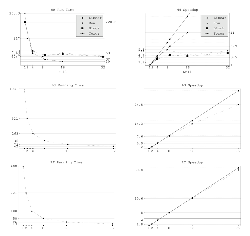
5.2 Benchmarking Haskell_# with Loild’s Benchmark Suite

The benchmarking results of Haskell_# implementations of Matrix Multiplication (MM), LinSolv (LS), and Ray Tracer (RT), based on Eden and GpH versions presented in [59], are shown in Figure 26. The parameters are described on Table 5. Since the cluster used has nodes about three times as fast as than nodes of the cluster used in Loild’s measures, the size of the problem instance of MM and RT used in this paper are larger. This attempts to approximate the sequential run-time of original measures and the increase of granularity of computations. For LS, however, the same problem size is used since its scalability is less sensitive to variations in problem size.

The speedup curves of LS and RT are nearly linear, while the speedup curve of MM is negatively affected due to the overhead caused by marshalling large nested lists of integers. For row and block clustering of MM, the times measured in 16 processors were little worse than those obtained for 8 and 9 processors, respectively. The marshalling overhead could be minimized by use of Haskell arrays instead of lists to represent matrices. The Haskell_# implementations for NPB kernels, where the amount of exchanged data is far larger, evidence this hypothesis. The toroidal version of MM yields a better performance scalability in comparison to row and block clustering, once the amount of data transmitted is comparatively smaller.

Table 5: Problem Instance Parameters for Loild’s Benchmark Suite

Matrix Multiplication	$960\times 960$ matrices of integers with maximum
	value of 65536.
LinSolv	Dense $62\times 62$ matrix of arbitrary precision
	integers with maximum value of $2^{16}-1$ .
Ray Tracer	An $1000\times 1000$ image (in pixels) with a scene
	comprising 640 spheres.

It is important to observe that measures of LS and RT for 32 processors were obtained on dual processing mode across 16 nodes of the cluster. Unexpected additional overhead was observed when executing MPI programs using the dual mode processing capabilities. This effect was more easily observed when measuring the run time of Haskell $\#$ versions of NPB kernels CG and IS, probably due to the large amount of data exchanged between processors in collective communication. Because of that, the results for NPB with 32 processors was not presented. Best speedup for LS and RT were expected for 32 non-dual processors. For that reason, in following discussion, the measures with 16 processors is used as a reference for comparing benchmarks of Haskell_# to benchmarks of GpH, Eden, and PMLS.

Comparing Haskell_# results to the best ones obtained for Eden, GpH, and PNML described in [59], one may observe that Haskell_# results are slightly better in all cases. For example, MM using toroidal solution obtains a speedup of 11.0 on 16 processors, while a speedup of approximately 5.0 was the best obtained in Eden toroidal solution. For LS, the speedup obtained in Haskell_# is 14.3 on 16 processors, while the best speedup obtained in Eden version was 14.0. For RT, a speedup of 15.6 was obtained by Haskell_# on 16 processors, while 15.1 was the best speedup obtained in PMLS version.

The results presented herein are not yet sufficient to conclude that Haskell_# programs are always more efficient than their GpH, Eden and PMLS versions. The two compared benchmarks were obtained for distinct architectures and using different problem sizes. However, the results presented in this paper evidence that Haskell_# implementation presents comparable behavior to well-known and mature implementations of parallel functional languages, such as GpH, Eden and PMLS. The results obtained are not surprising, since Haskell_# run-time system is very light in relation to the complex parallel run-time systems of GpH, Eden, and PMLS, which try to hide some parallel management details from programmers at different degrees. Decades of experience in parallel languages design have shown that as explicit as it is a general parallel language, assuming that it has an efficient implementation, best scalability is obtained using a simpler run-time system. The combination of the results obtained in this paper and in [59] only confirm this hypothesis. In this sense, Haskell_# is the most explicit of all, followed by Eden, PMLS and GpH, respectively.

6 Conclusions and Lines for Further Work

This paper introduces Haskell_#, a coordination language for describing parallel execution of functional computations in Haskell. Haskell_# intends to raise the level of abstraction in explicit message-passing parallel programming on distributed architectures, such as clusters, for the development of large scale parallel scientific computing applications. Motivating examples, implementation issues and performance figures of Haskell_# benchmarks are also presented.

After some years of design, implementation and evaluation, Haskell_# has reached some maturity. Several works unfoldings are on progress. Firstly, a parallel programming environment based on Haskell_# have been prototyped in JAVA, including the support for programming with visual abstractions, integration to Petri net tools for animation, proving of formal properties, and performance evaluation of programs. It is also under development the use of network simulators, such as Network Simulator (NS) [31] for simulating the performance of parallel programs. Such tool will allow to study the effect of modifications to network characteristics on performance of parallel programs. This work has important impact on studying behavior of Haskell_# programs whenever executing on grids.

Since HCL is a coordination language orthogonal to Haskell, it is conceptually possible to use other languages, in alternative to Haskell, for programming functional modules. The parallel programming environment under development assumes that Haskell is the ideal language for specifying, prototyping and evaluating the formal properties of parallel programs. Once parallel composition is proved be safe, programmers may implement the functional modules using a language more appropriate for implementing the functionality of the simple components. For example, numerical intensive functional modules could be implemented in Fortran, while sorting of large amount of numbers in parallel may be implemented in C. JAVA can be used for programming functional modules that make access to some database. This kind of multi-lingual compositional approach is a further development. One important design difficult with multilingual approach is to maintain the orthogonality between languages used at coordination and computations levels in absence of lazy and higher-order functional programming. Imperative languages, for example, do not allow to hide the control flow. It is intended to use techniques from aspect oriented programming (AOP) for addressing this matter. In this direction, parallel composition could be treated as an aspect of programming. The recent appearance of heterogeneous versions of MPI [84] is important for making feasible a multi-lingual approach for Haskell_#.

An even more relevant important topic to be addressed is to develop cost models for Haskell_# skeletons, incorporating the possibility of overlapping them, and to use it for allowing Haskell_# compiler to make automatic decisions, such as better allocation of processes to processors, use of special primitives, and special restrictions on communication modes, such as the size of buffers. However, a recent idea is to design a meta-language for programmers to teach explicitly Haskell $\#$ compiler on how to generate the appropriate code for a given skeleton or a combination of skeletons. The latter approach is more in tune with Haskell_# design premisses. However, it is not difficult to see that the two lines could be combined.

Further developments will address grid enabled implementations of Haskell_#. A grid enabled version of MPI, such as the recently proposed MPICH-G2 [49], might be used.

References

[1] F. Arbab, P. Ciancarini, and C. Hankin. Coordination Languages for Parallel Programming. Parallel Computing, 24(7):989–1004, 1998.
[2] D. H. Bailey and et al. The NAS Parallel Benchmarks. International Journal of Supercomputing Applications, 5(3):63–73, 1991.
[3] D. H. Bailey, T. Harris, W. Shapir, R. van der Wijngaart, A. Woo, and M. Yarrow. The NAS Parallel Benchmarks 2.0. Technical Report NAS-95-020, NASA Ames Research Center, December 1995. http://www.nas.nasa.org/NAS/NPB.
[4] M. Baker, R. Buyya, and D. Hyde. Cluster Computing: A High Performance Contender. IEEE Computer, 42(7):79–83, July 1999.
[5] S. Balay, K. Buschelman, W. Gropp, D. Kaushik, M. Knepley, L. C. McInnes, B. Smith, and H. Zhang. PETSc Users Manual. Technical Report ANL-95/11 Revision 2.1.3, Argonne National Laboratory, Argonne, Illinois, 1996. http://www.mcs.anl.gov/petsc.
[6] E. Barscz, R. Fatoohi, V. Venkatakrishnan, and S. Weeratunga. Solution of Regular, Sparse Triangular Systems on Vector and Distributed-Memory Multiprocessors. Technical Report NAS RNR-93-007, NASA Ames Research Center, April 1993.
[7] G. Baumgartner, Bernholdt D. E., D. Cociorva, R. Harrison, S. Hirata, C. Lam, M. Nooijen, R. Pitzer, J. Ramanujam, and P. Sadayappan. A High-Level Approach to Synthesis of High-Performance Codes for Quantum Chemistry. In 2002 ACM/IEEE conference on Supercomputing, pages 1–10, 2002. Baltimore, Maryland, USA.
[8] D. J. Becker, T. Sterling, D. Savarese, J. E. Dorban, U. A. Ranawak, and C. V. Packer. Bewoulf: A Parallel Workstation for Scientific Computation. In 1995 International Conference on Parallel Processing, 1995.
[9] G. Bell and J. Gray. What’s the Next in High Performance Computing. Communications of the ACM, 45(2):91–95, 2002.
[10] D. E. Bernholdt, J. Nieplocha, and P. Sadayappan. Raising Level of Programming Abstraction in Scalable Programming Models. In IEEE International Conference on High Performance Computer Architecture (HPCA), Workshop on Productivity and Performance in High-End Computing (P-PHEC), pages 76–84. Madrid, Spain, IEEE Computer Society, 2004.
[11] M. Bertozzi, G. Chiola, G. Ciaccio, G. Conte, P. Marenzoni, A. Poggi, and P. Rossi. DISCO Report on the State-of-the-Art of PC Cluster Computing. Technical Report DISI-TR-98-09, DISI, Universitá de Genova, December 1998.
[12] E. Best, J. Esparza, B. Grahlmann, S. Melzer, S. Rmer, and F. Wallner. The PEP Verification System. In Workshop on Formal Design of Safety Critical Embedded Systems (FEmSys’97), 1997.
[13] J. M. Bishop. Languages for Configuration Programming: A Comparison. Technical Report 94-04, University of Pretoria, 1994.
[14] S. Breitinger, R. Lógen, Y. Ortega Mallén, and R. Peña. Eden - The Paradise of Functional Concurrent Programming. Lecture Notes in Computer Science (EUROPAR’96), 1123:710–713, 1996.
[15] J. F. Briesmeister. MCNP - A General Monte Carlo N-Particle Transport Code. Technical Report LA-12625-M, Los Alamos National Laboratory, 1993.
[16] W. H. Burge. Recursive Programming Techniques. Addison-Wesley Publishers Ltd., 1975.
[17] G. Burns, R. Daoud, and J. Vaigl. LAM: An Open Cluster Environment for MPI. In Proceedings of Supercomputing Symposium, pages 379–386, 1994.
[18] F.W. Burton. Functional Programming for Concurrent and Distributed Computing. Computer Journal, 30(5):437–450, 1987.
[19] R. Buyya (ed.). High Performance Cluster Computing: Architectures and Systems. Prentice Hall, 1999.
[20] R. Buyya (ed.). High Performance Cluster Computing: Programming and Applications. Prentice Hall, 1999.
[21] F. H. Carvalho Junior and R. D. Lins. Topological Skeletons in Haskell_#. In International Parallel and Distributed Processing Symposium (IPDPS). IEEE Press, April 2003. 8 pages.
[22] F. H. Carvalho Junior, R. D. Lins, and R. M. F. Lima. Parallelising MCP-Haskell_# for Evaluating $Haskell_{\#}$ Parallel Programming Environment. In UnB, editor, 13th Brazilian Symposium on Computer Architecture and High-Performance Computing (SBAC-PAD 2001), September 2001.
[23] F. H. Carvalho Junior, R. D. Lins, and R. M. F. Lima. Translating Haskell_# Programs into Petri Nets. Lecture Notes in Computer Science (VECPAR’2002), 2565:635–649, 2002.
[24] M. (editor) et all Chakravarty. The Haskell 98 Foreign Function Interface (FFI) 1.0 (An Addendum to Haskell 98 Report). Glasgow University, Departament of Computing, Functional Programming Research Group, 2002.
[25] M. Cole. Algorithm Skeletons: Structured Management of Paralell Computation. Pitman, 1989.
[26] J. Darlington, Y. Guo, H.W. To, and J. Yang. Functional Skeletons for Parallel Coordination. Lecture Notes in Computer Science, 966:55–68, 1995.
[27] F. DeRemer and H. H. Kron. Programming-in-the-Large versus Programming-in-the-small. IEEE Transactions on Software Engineering, pages 80–86, June 1976.
[28] J. Dongarra, I. Foster, G. Fox, W. Gropp, K. Kennedy, L. Torczon, and A. White. Sourcebook of Parallel Computing. Morgan Kauffman Publishers, 2003.
[29] J. Dongarra, S. W. Otto, M. Snir, and D. Walker. An Introduction to the MPI Standard. Technical Report CS-95-274, University of Tennessee, January 1995. http://www.netlib.org/tennessee/ut-cs-95-274.ps.
[30] C. Dornan, I. Jones, and S. Marlow. Alex User Guide, 2003. http://www.haskell.org/alex.
[31] K. Fall and K. Varadhan. The NS Manual (formely NS Notes and Documentation). Technical report, The VINT Project, A Collaboration between researchers at UC Berkeley, LBL, USC/ISI, and Xerox PARC, April 2002.
[32] High Performance Fortran Forum. High Performance Fortran, Language Specification, Version 2.0, January 1997.
[33] I. Foster. Compositional Parallel Programming Languages. ACM Transactions on Programming Languages and Systems, 18(4):454–476, 1985.
[34] I. Foster and C. Kesselman. The Grid 2: Blueprint for a New Computing Infrastructure. M. Kauffman, 2004.
[35] D. Gelernter and N. Carriero. Coordination Languages and Their Significance. Communications of the ACM, 35(2):97–107, February 1992.
[36] R. German. SPNL: Processes as Language-Oriented Building Blocks of Stochastic Petri Nets. In 9th Conference on Computer Performance Evaluation, Modelling Techniques and Tools, pages 123–134. Springer Verlag, 1997.
[37] W. Gropp, E. Lusk, N. Doss, and A. Skjellum. A High-Performance, Portable Implementation of the MPI Message Passing Interface Standard. Parallel Computing, 22(6):789–828, 1996.
[38] M. M. Hamdan. A Combinational Framework for Paralell Programming Using Skeleton Functions. PhD thesis, Department of Computing and Electrical Engineering, Hariot-Watt University, January 2000.
[39] J. Hammes, O. Lubeck, and W. Böhm. Comparing Id and Haskell in a Monte Carlo Photon Transport Code. Journal of Functional Programming, pages 283–316, July 1995.
[40] K. Hammond, J. Berthold, and R. Loogen. Automatic Skeletons in Template Haskell. Parallel Processing Letters, 13(3), 2003.
[41] K. Hammond and G. Michaelson. Research Directions in Parallel Functional Programming. Springer-Verlag, 1999.
[42] C. Herrman and C. Lengauer. A Higher-Order Language for Dividing and Conquer. Paralell Processing Letters, 10(2-3):239–250, 2000.
[43] C. A. R. Hoare. Communicating Sequential Processes. Prentice-Hall International Series in Computer Science, 1985.
[44] P. Hudak. Serial Combinators: “Optimal” Grains of Parallelism. In FPCA’85, pages 382–399, September 1985.
[45] P. Hudak. Para-Functional Programming in Haskell. Parallel Functional Languages and Compilers, B. K. Szymanski, Ed. ACM Press, New York, pages 159–196, 1991.
[46] Inmos. Occam Programming Manual. Prentice-Hall, C.A.R. Hoare Series Editor, 1984.
[47] T. Ito and Y. Nishitani. On Universality of Concurrent Expressions with Synchronization Primitives. Theoretical Computer Science, 19:105–115, 1982.
[48] N. Karonis, B. D. Supinski, I. Foster, W. Gropp, E. Lusk, and J. Bresnahan. Exploiting Hierarchy in Parallel Computer Networks to Optimize Collective Operation Performance. In 14th International Parallel and Distributed Processing Symposium, pages 377–384, 2000. Los Alamitos, CA, USA.
[49] N. Karonis, B. Toonen, and I. Foster. MPICH-G2: A Grid-enabled Implementation of the Messaging Passing Interface. Journal of Parallel and Distributed Computing, 63(5):551–563, 2003.
[50] O. Kaser, C.R. Ramakrishnan, I. V. Ramakrishnan, and R. C. Sekar. Equals - A Fast Parallel Implementation of a Lazy Language. Journal of Functional Programming, 7(2):183–217, March 1997.
[51] P. Kelly. Functional Programming for Loosely-coupled Multiprocessors. Research Monographs in Parallel and Distributed Computing, MIT Press, 1989.
[52] G. Kiczales, J. Lamping, Menhdhekar A., Maeda C., C. Lopes, J. Loingtier, and J. Irwin. Aspect-Oriented Programming. In Lecture Notes in Computer Science (Object-Oriented Programming 11th European Conference – ECOOP ’97), volume 1241, pages 220–242. Springer-Verlag, November 1997.
[53] J. Krammer. Distributed Software Engineering. In IEEE Computer Society Press, editor, Proc. 16th IEEE International Conference on Software, 1994.
[54] Lauer M. Computing by Homomorphic Images. In G. Buchberger, G. E. Collins, R. Loos, and Albrecht R., editors, Computer Algebra - Symbolic and Algebraic Computation, pages 139–168. Springer, 1982.
[55] R. M. F. Lima. Haskell_# - Uma Linguagem Funcional Paralela - Ambiente de Programação, Implementação e Otimização. PhD thesis, Centro de Informáica, UFPE, July 2000.
[56] R. M. F. Lima and R. D. Lins. Translating HCL Programs into Petri Nets. In Proceedings of the 14th Brazilian Symposium on Software Engineering, 2000.
[57] R. D. Lins. Functional programming and parallel processing. In 2nd International Conference on Vector and Parallel Processing - VECPAR‘96 - LNCS 1215 Springer-Verlag, pages 429–457, September 1996.
[58] J. D. Lipson. Chinese Remainder and Interpolation Algorithms. In SYMSAM’71 - Symposium on Symbolic and Algebraic Manipulation, pages 372–391. Academic Press, 1971.
[59] H.-W. Loidl, S. Priebe, A. J. Rebon, P. W. Trinder, F. Rubio, N. Scaife, K. Hammond, S. Horiguchi, L. Loogen, G. J. Michaelson, and R. Pe na. Comparing Parallel Functional Languages: Programming and Performance. Higher-Order and Symbolic Logic, 16(3):203–251, September 2003.
[60] H. W. et al Loidl. LinSolv: A Case Study in Strategic Parallelism. In Glasgow Workshop on Functional Programming, pages 15–17, 1997.
[61] S. Lucco and O. Sharp. Delirium: An Embedding Coordination Language. In Proceedings of the 1990 Conference on Supercomputing, pages 515–524. IEEE Computer Society Press, 1990.
[62] S. Marlow and A. Gill. Happy User Guide, 2001. http://www.haskell.org/happy.
[63] Message Passing Interface Forum. MPI: A Message-Passing Interface Standard. International Journal of Supercomputer Applications and High Performance Computing, 8(3-4):169–416, 1994.
[64] G. Michaelson, N. Scaife, and P. King. Nested Algorithmic Skeletons for Higher Order Functions. Parallel Algorithms and Applications, 16:181–206, 2001.
[65] E. E. Miller and R. H. Katz. Input/Output Behavior of Supercomputing Applications. In Proceedings of Conference Supercomputing’91, pages 567–576, November 1991.
[66] J. Nieplocha, R. J. Harrison, and R. J. Littlefield. Global Arrays: A Non-Uniform-Memory-Access Programming Model for High-Performance Computers. The Journal of Supercomputing, 10(2):169–189, 1996.
[67] OpenMP Architecture Review Board. OpenMP: Simple, Portable, Scalable SMP Programming, 1997.
[68] H. Ossher and P. Tarr. Multi-Dimensional Separation of Concerns and the Hyperspace Approach. In Proceedings of the Symposium on Software Architectures and Component Technology: The State of the Art in Software Development. Kluwer Academics, June 2000. University of Twente, Enschede, The Netherlands.
[69] C. Pareja, R. Pe na, F. Rubio, and C. Segura. Optimizing Eden by Transformation. In S. Gilmore, editor, Trends in Functional Programming (2nd Scottish Functional Programming Workshop), volume 1, chapter 4, pages 39–52. Intellect Books, 2000.
[70] B. K. Pasquale and G. Plyzos. A Statis Analysis of I/O Characterization of Scientific Applications in a Production Workload. In Proceedings of Conference Supercomputing’93, pages 388–397, November 1993.
[71] J. L. Peterson. Petri Net Theory and Modeling of Systems. Prentice-Hall, 1981.
[72] C. A. Petri. Kommunikation mit Automaten. Technical Report RADC-TR-65-377, Griffiths Air Force Base, New York, 1(1), 1966.
[73] S. L. Peyton Jones, C. Clack, and J. Salkild. GRIP - A High-Performance Architecture for Parallel Graph Reduction. FPCA’87: Conference on Functional Programming Languages and Computer Architecture - Springer-Verlag LNCS 274, pages 98–112, 1987.
[74] S. L. Peyton Jones, A. Gordon, and S. Finne. Concurrent Haskell. In POPL’96 - Symposium on Principles of Programming Languages, ACM Press, pages 295–308, January 1996.
[75] S. L. Peyton Jones and J. (editors) Hughes. Report on the Programming Language Haskell 98, A Non-strict, Purely Functional Language, February 1999.
[76] M. J. Plasmeijer and M. van Eekelen. Functional Programming and Parallel Graph Rewriting. Addison-Wesley Publishers Ltd., 1993.
[77] Post D. E. The Coming Crisis in Computational Science. In IEEE International Conference on High Performance Computer Architecture (HPCA), Workshop on Productivity and Performance in High-End Computing (P-PHEC). Madrid, Spain, 2004.
[78] M. Quinn. Parallel Computing. McGraw-Hill, 1994.
[79] F. A. Rabhi and S. Gorlatch. Patterns and Skeletons for Parallel and Distributed Computing. Springer, 2002.
[80] S. Roch and P. Starke. Manual: Integrated Net Analyzer Version 2.2, 1999.
[81] P. M. Sansom and S. L. Peyton Jones. Time and Space Profiling for Non-Strict, Higher-Order Functional Languages. In Proceedings of the 22nd ACM SIGPLAN-SIGACT Symposium on Principles of Programming Languages, pages 355–366. ACM Press, 1995.
[82] V. Sarkar, C. Williams, and K. Ebcio $\breve{g}$ lu. Application Development Productivity Challenges for High-End Computing. In IEEE International Conference on High Performance Computer Architecture (HPCA), Workshop on Productivity and Performance in High-End Computing, pages 14–18, 2004.
[83] D. B. Skillicorn and D. Talia. Models and Languages for Parallel Computation. ACM Computing Surveys, 30:123–169, June 1998.
[84] J. M. Squyres, A. Lumsdaine, W. L. George, J. G. Hagedorn, and J. E. Devaney. The interoperable message passing interface (IMPI) extensions to LAM/MPI. In Proceedings, MPIDC’2000, March 2000.
[85] F. Taylor. Parallel Functional Programming by Partitioning. PhD Thesis, Department of Computing, Imperial College of Science, Technology and Medicine, University of London, January 1997.
[86] P. Trinder, K. Hammond, J. S. Mattson Junior, A. S. Partridge, and S. P. L. Jones. GUM: A Portable Parallel Implementation of Haskell. In PLDI’96 - Programming Languages Design and Implementation, pages 79–88, 1996.
[87] P. W. Trinder, H-W. Loidl, and R. F. Pointon. Parallel and Distributed Haskells. Journal of Functional Programming, 12(4/5):469–510, July 2002.
[88] P.W. Trinder, K. Hammond, and H. W. Loidl. Algorithm + Strategy = Parallelism. Journal of Functional Programming, 8(1):23–60, January 1998.
[89] R. Valk and G. Vidal Naquet. Petri Nets and Regular Languages. Journal of Computer and System Sciences, 23:299–325, 1981.
[90] P. Wadler. Monads for Functional Programming. Advanced Functional Programming, LNCS 925, Springer-Verlag, 1995. http://cm.bell-labs.com/cm/cs/who/wadler/papers/marktoberdorf/marktoberdorf.ps.gz.
[91] Weber M. and Kindler E. The Petri Net Markup Language. Lecture Notes in Computer Science, 2002. Submitted for publication in april 2002.
[92] A. Zimmermann, J. Freiheit, R. German, and G. Hommel. Petri Net Modelling and Performability Evaluation with TimeNET 3.0. In 11th Int. Conf. on Modelling Techniques and Tools for Computer Performance Evaluation (TOOLS’2000), pages 188–202. Lecture Notes in Computer Sciente, 2000.

Appendix A The Formal Syntax of HCL

In what follows, it is described a context-free grammar for HCL, the Haskell_# Configuration Language, whose syntax and programming abstractions were informally presented in Section 2. Examples of HCL configurations and their meanings were presented in Sections 2 and 3. The notation employed here is similar to that used for describing syntax of Haskell 98 [75]. Indeed, some non-terminals from that grammar are reused here, once some Haskell code appears in HCL configurations. They are faced italic and bold. A minor difference on notation resides on the use of $(\dots)^{?}$ , instead of $[\dots]$ , for describing optional terms. For simplicity, notation for indexed notation is ignored from the description of formal syntax of HCL. It may be resolver by a pre-processor, before parsing.

A.1 Top-Level Definitions

configuration	$\rightarrow$ header declaration₁ $\dots$ declaration_n ( $n\geq 0$ )
header	$\rightarrow$ component ID static_parameter_list^? component_interface^?
static_parameter_list	$\rightarrow$ $<$ ID₁ $\dots$ ID_n $>$ ( $n\geq 0$ )
component_interface	$\rightarrow$ ports_naming
declaration	$\rightarrow$	import_decl	$\mid$ use_decl	$\mid$ iterator_decl	$\mid$ interface_decl
	$\mid$	unit_decl	$\mid$ assign_decl	$\mid$ replace_decl	$\mid$ channel_decl
	$\mid$	unify_decl	$\mid$ factorize_decl	$\mid$ replicate_decl	$\mid$ bind_decl
	$\mid$	haskell_code

A.2 Use Declaration

use_decl

\rightarrow

use use_spec

use_spec

\rightarrow

\mid

id.use_spec

\mid

id.{ use_spec₁ ,

\dots

, use_spec_n } (

n\geq 1

)

A.3 Import Declaration

import_decl

\rightarrow

impdecl

A.4 Iterator Declaration

iterator_decl

\rightarrow

iterator id₁,

\dots

, id_n range [ numeric_exp , numeric_exp ] (

n\geq 1

)

A.5 Interface Declaration

interface_decl	$\rightarrow$ interface (context $=>$ )^? ID tyvar₁ $\dots$ tyvar_k interface_spec
interface_spec	$\rightarrow$	interface_ports_spec
		(where : interface_inheritance)^? (behavior : behavior_expression)^?

A.5.1 Interface Ports Description

interface_ports_spec	$\rightarrow$ port_spec_list - $>$ port_spec_list
port_spec_list	$\rightarrow$ port_spec $\mid$ ( port_spec₁ , $\dots$ , port_spec_n ) ( $n\geq 2$ )
port_spec	$\rightarrow$ id ()^? (:: atype*)^? $\mid$ id

A.5.2 Interface Composition

interface_inheritance	$\rightarrow$ interface_slice₁ # $\dots$ # interface_slice_k ( $k\geq 1$ )
interface_slice	$\rightarrow$ id @ ID $\mid$ ID ports_naming_composition
ports_naming_composition	$\rightarrow$	ports_naming
	$\mid$	( ports_naming₁ # $\dots$ # ports_naming_n) ( $n\geq 1$ )
ports_naming	$\rightarrow$ port_naming_list - $>$ port_naming_list
port_naming_list	$\rightarrow$ id $\mid$ ( id₁ , $\dots$ , id_n) ( $n\geq 1$ )

A.5.3 Interface Behavior


behavior_expression	$\rightarrow$ (sem id₁ , $\dots$ , id_n)^? : action ( $n\geq 1$ )
action	$\rightarrow$	par { action₁ ; $\dots$ ; action_n } $\mid$ seq { action₁ ; $\dots$ ; action_n }
	$\mid$	alt { action₁ ; $\dots$ ; action_n } $\mid$ repeat action condition^?
	$\mid$	if condition then action else action
	$\mid$	id ! $\mid$ id ? $\mid$ signal id $\mid$ wait id ( $n\geq 2$ )
condition	$\rightarrow$ until disjunction $\mid$ counter numeric_exp
disjunction	$\rightarrow$ conjunction₁ ‘ $\mid$ ’ $\dots$ ‘ $\mid$ ’ conjunction_n ( $n\geq 1$ )
sync_conjunction	$\rightarrow$ $\langle$ simple_conjunction $\rangle$ $\mid$ simple_conjunction
simple_conjunction	$\rightarrow$ id $\mid$ ( id₁ & $\dots$ & id_n ) ( $n\geq 1$ )

A.6 Unit Declaration

unit_decl	$\rightarrow$ unit unit_spec
unit_spec	$\rightarrow$ ()^? id (# unit_interface)^? (wire wf_setup₁ , $\dots$ , wf_setup*_n)^?
unit_interface	$\rightarrow$ ID ports_naming_composition^? $\mid$ interface_spec
wf_setup	$\rightarrow$	id (group_type group_spec)^? (: wire_function)^?
group_spec	$\rightarrow$ { id₁, $\dots$ , id_n } $\mid$ * numeric_exp
group_type	$\rightarrow$ any $\mid$ all
wire_function	$\rightarrow$ ? $\mid$ exp

A.7 Assignment Declaration

assign_decl	$\rightarrow$ assign assigned_component to assigned_unit
assigned_component	$\rightarrow$ ID actual_parameter_list^? ports_naming_composition^?
actual_parameter_list	$\rightarrow$ $<$ numeric_exp₁ , $\dots$ , numeric_exp_n $>$ ( $n\geq 1$ )
assigned_unit	$\rightarrow$ qid ports_naming_composition^?

A.8 Replace Declaration

replace_decl

\rightarrow

replace qid ports_naming_composition^? by operand_unit

A.9 Channel Declaration

channel_decl	$\rightarrow$ connect qid - $>$ qid to qid $<$ - qid , comm_mode
comm_mode	$\rightarrow$ synchronous $\mid$ buffered numeric_exp $\mid$ ready

A.10 Unification Declaration

unify_decl	$\rightarrow$ unify	operand_unit₁ , $\dots$ , operand_unit_n to unit_spec
		adjust wire wf_setup₁ , $\dots$ , wf_setup_k ( $n\geq 2,\ k\geq 1$ )
operand_unit	$\rightarrow$ qid # interface_pattern₁ $\dots$ # interface_pattern_n ( $n\geq 1$ )
interface_pattern	$\rightarrow$ port_pattern_list - $>$ port_pattern_list $\mid$ id
port_pattern_list	$\rightarrow$ pattern $\mid$ ( pattern₁ , $\dots$ , pattern_n )
pattern	$\rightarrow$ id $\mid$ @ qid $\mid$ _ $\mid$ __

A.11 Factorization Declaration

factorize_decl $\rightarrow$ factorize	operand_unit to unit_spec₁ $\dots$ unit_spec_n
	adjust wire wf_setup₁ , $\dots$ , wf_setup_k ( $n\geq 2,\ k\geq 1$ )

A.12 Replication Declaration

replicate_decl $\rightarrow$ replicate	operand_unit₁ , $\dots$ , operand_unit_n into numeric_exp
	adjust wire wf_setup₁ , $\dots$ , wf_setup_k ( $n\geq 2,\ k\geq 1$ )

A.13 Bind Declaration

bind_declaration

\rightarrow

bind qid -

>

qid to -

>

\mid

bind qid

<

- qid to

<

- id

A.14 Miscelaneous

haskell_code

\rightarrow

topdecls

qid

\rightarrow

id₁ ‘.’

\dots

‘.’ id_n (

n\leq 2

)

qID

\rightarrow

ID₁ ‘.’

\dots

‘.’ ID_n (

n\leq 2

)

Appendix B An Algebraic Semantics for Haskell_# Components

This appendix presents an algebra intending to formalize semantics of Haskell_# programming abstractions at coordination level. A Haskell_# component H may be defined by an algebra with the following elements:

$\begin{array}[]{l}\\ \textbf{H}=<\textsc{G},\textsc{R},\textsc{C}>\\ \\ \end{array}$

where G is a set of generators, R is a set of relations on generators, and C is a set of restrictions on relations, defined as following:

\textsc{G}=\left\{\begin{array}[]{lr}C,&\mbox{\it composed components}\\ S,&\mbox{\it simple components}\\ U,&\mbox{\it units}\\ G,&\mbox{\it ports groupings}\\ P,&\mbox{\it individual ports}\\ R,&\mbox{\it kinds of processes: {repetitive} or {non-repetitive}}\\ D,&\mbox{\it port directions: {input} or {output}}\\ T,&\mbox{\it port type: {any} or {all}}\\ M&\mbox{\it communication modes: {synchronous}, {buffered} or {ready}}\\ \end{array}\right\}

\textsc{R}=\left\{\begin{array}[]{lr}\omega:\{\star\}\rightarrow C\cup S&\mbox{main component}\\ \delta:C\rightarrow 2^{U},&\mbox{\it units that comprise a component}\\ \psi:P\rightarrow P,&\mbox{\it association of ports to argument/return points}\\ \gamma:U\rightarrow C\cup S,&\mbox{\it component associated to a unit}\\ \pi:G\rightarrow U\times D,&\mbox{\it unit of a port grouping}\\ \beta:U\rightarrow G^{*},&\mbox{\it behavior of a unit}\\ \tau:Q\rightarrow 2^{P}\times T,&\mbox{\it grouping of ports}\\ \rho:U\rightarrow R,&\mbox{\it type of process}\\ \nu:P\times P\times M&\mbox{\it communication channels}\\ \lambda:G\rightarrow Nat&\mbox{\it nesting factor of a stream port}\\ \iota:U\rightarrow 2^{G}\times 2^{G^{*}}&\mbox{\it interface of a unit}\end{array}\right\}

\textsc{C}=\{\mathbf{R_{1}},\mathbf{R_{2}},\mathbf{R_{3}},\mathbf{R_{4}},\mathbf{R_{5}},\mathbf{R_{6}},\mathbf{R_{7}},\mathbf{R_{8}},\mathbf{R_{9}},\mathbf{R_{10}},\mathbf{R_{11},\mathbf{R_{12}}}\}

A Haskell_# program is a component that may execute. Essentially, it does not have virtual units in its composition (it is not a partial skeleton). All units are assigned to a component ( $\forall u:u\in U:(\exists c:c\in C\cup S:\gamma(u)=c)$ ).

In what follows, the restrictions from $R_{1}$ to $R_{12}$ are described. They are formulas in predicate logic (predicate) of the following form $(\forall b_{1},b_{2},\dots,b_{n}:R:P)$ or $(\exists b_{1},b_{2},\dots,b_{n}:R:P)$ , where $\forall$ and $\exists$ are the usual existential quantifier, $b_{i}$ , $1\leq i\leq n$ , are bound variables, $R$ is a formula that specifies the set of values of bound variables, and $P$ is a logical predicate.

The restriction $\mathbf{R_{1}}$ states that component $\omega$ (main component) is the only component that is not assigned to any unit:

\footnotesize\begin{array}[]{c}\mathbf{R_{1}}\vdash\forall u:u\in U:\gamma(u)\neq\omega\\ \end{array}

(1)

$\mathbf{R_{2}}$ states that cyclic dependencies may not occur in component hierarchy:

\footnotesize\begin{array}[]{c}\mathbf{R_{2}}\vdash\forall u:u\in U\wedge\gamma(u)\neq\bot:u\notin(\overline{\delta}\circ\gamma)(u)\\ \\ \begin{array}[]{lll}\mathbf{where}:&\overline{\delta}(s)=\emptyset&s\in S\\ &\overline{\delta}(c)=\bigcup_{u\in\delta(c)}(\overline{\delta}\circ\gamma)(u)&c\in C\end{array}\par\end{array}

(2)

$\mathbf{R_{3}}$ states that a cluster is repetitive whenever all units belonging to its assigned component are repetitive:

\footnotesize\begin{array}[]{c}\mathbf{R_{3}}\vdash\forall u:u\in U\wedge(\exists c:c\in C:\gamma(u)=c\wedge\delta(c)\neq\emptyset):\\ \rho(u)=\mbox{\bf Repetitive}\Leftrightarrow(\forall\overline{u}:\overline{u}\subseteq(\delta\circ\gamma)(u)):\rho(\overline{u})=\mbox{\bf Repetitive})\\ \\ \end{array}

(3)

$\mathbf{R_{4}}$ state that groups of ports are disjoint, $\mathbf{R_{5}}$ states that all individual ports belong to a group of ports, and $\mathbf{R_{6}}$ states that groups of ports must not be empty:

\footnotesize\begin{array}[]{c}\mathbf{R_{4}}\forall g,g^{\prime}:g,g^{\prime}\in G:\pi(g)\cap\pi(g^{\prime})=\emptyset\\ \\ \mathbf{R_{5}}\forall p\ \exists g:p\in P\wedge g\in G:p\in\tau(g)\\ \\ \mathbf{R_{6}}\forall g:g\in G:\tau(g)\neq\emptyset\\ \end{array}

(4)

In the algebra, all ports are treated as non-empty groups. Thus, an individual port in a Haskell_# program is represented as a group containing an unique port. The restrictions above makes possible to define a “inverse” relation $\overline{\tau}$ ³³3This is not the strict mathematical notion of inverse function, from set theory., such that $\overline{\tau}$ (p) returns the group $g$ that $p$ belongs. It is useful for simplifying next formulations.

Restrictions $\mathbf{R_{7}}$ , $\mathbf{R_{8}}$ , and $\mathbf{R_{9}}$ specifies rules for formation of channels. Respectively, they say that channels are point-to-point, unidirectional and have the same nesting factors:

\footnotesize\begin{array}[]{c}\mathbf{R_{7}}\vdash(p^{o}_{1},p^{i}_{1},m)\in\nu\wedge(p^{o}_{2},p^{i}_{2},m)\in\nu\Rightarrow p^{o}_{1}=p^{o}_{2}\Leftrightarrow p^{i}_{1}=p^{i}_{2}\\ \\ \mathbf{R_{8}}\vdash(p^{o},p^{i},m)\in\nu\Rightarrow(\exists u,u^{\prime}:u,u^{\prime}\in U:(\pi\circ\overline{\tau})(p^{o})=(u,\mbox{\bf Output})\wedge(\pi\circ\overline{\tau})(p^{i})=(u^{\prime},\mbox{\bf Input}))\\ \\ \mathbf{R_{9}}\vdash(p^{o},p^{i},m)\in\nu\Rightarrow(\lambda\circ\overline{\tau})(p^{o})=(\lambda\circ\overline{\tau})(p^{i}))\\ \end{array}

(5)

Let $u$ be a cluster ( $\gamma(u)\subseteq C$ ) and $p$ be an individual port belonging to group $g$ , such that $\pi(g)=(u,d)$ , for $d\in D$ ( $p$ belongs to interface of $u$ ). The restriction $\mathbf{R_{10}}$ ensures that $\psi(p)$ (argument or exit point of $\gamma(u)$ ) is a port with the same direction of $p$ belonging to interface of unit $u^{\prime}$ , such that $u^{\prime}$ is a unit belonging to the component $\gamma(u)$ ( $u^{\prime}\in(\delta\circ\sigma)(u)$ ):

\footnotesize\begin{array}[]{c}\mathbf{R_{10}}\vdash\forall p:(\pi\circ\overline{\tau})(p)=(u,d)\wedge\gamma(u)\subseteq C:((\pi\circ\psi)(p)=(u^{\prime},d)\wedge u^{\prime}\in(\delta\circ\gamma)(u))\\ \end{array}

(6)

The restriction $\mathbf{R_{11}}$ defines the relation $\iota$ , which describes the interface of a unit:

\footnotesize\begin{array}[]{c}\mathbf{R_{11}}\vdash\iota(u)=<\{g\mid\pi(g)=(u,d)\},\beta(u)>\par\end{array}

(7)

$\mathbf{R_{12}}$ says that ports belonging to the same group whose communication pairs also belongs to the same groups are essentially the same port.

\footnotesize\begin{array}[]{c}\mathbf{R_{12}}\vdash(p^{o}_{1},p^{i}_{1},m_{1})\in\nu\wedge(p^{o}_{2},p^{i}_{2},m_{2})\wedge\tau(p^{o}_{1})=\tau(p^{o}_{2})\wedge\tau(p^{i}_{1})=\tau(p^{i}_{2})\Rightarrow p^{o}_{1}=p^{o}_{2}\wedge p^{i}_{1}=p^{i}_{2}\\ \end{array}

(8)

B.1 Formalizing Interfaces

This section formalizes homomorphism relations between interfaces, which are essential for formalizing unification and factorization operations in the next section.

B.1.1 The # Operator

The # operator allows for combining to interfaces, generating a new interface that inherits characteristics from original ones. It is defined as following:

\footnotesize\begin{array}[]{c}\mathbf{I_{1}}\#\ \mathbf{I_{2}}=<Q_{1}\cup Q_{2},B_{1}\hat{\cup}B_{2}>,\ \mathbf{where}\ \mathbf{I_{1}}=<Q_{1},B_{1}>\ \mbox{\bf and}\ \mathbf{I_{2}}=<Q_{2},B_{2}>\par\end{array}

(9)

The sets of ports from operand interfaces may overlap. The operator $\hat{\cup}$ generates a new formal language describing a behavior for interface $\mathbf{I_{1}}\#\mathbf{I_{2}}$ , which is compatible with original behavior of $\mathbf{I_{1}}$ and $\mathbf{I_{2}}$ , in separate. Given an interleaving operator $\odot$ , from concurrent expressions [47] and $\ell$ a function that returns the language generated by a concurrent expression, formal definition of $\hat{\cup}$ is:

\footnotesize\begin{array}[]{c}B_{1}\hat{\cup}B_{2}=\ell\left[(w_{1}\odot u_{1})\ s\ (w_{2}\odot u_{2})\ s\ {\dots}\ s\ (w_{n}\odot u_{n})\right],n\geq 1\\ \\ \mathbf{where}\\ \\ s\in Q_{1}\cap Q_{2}\\ \\ w_{1}\ s\ w_{2}\ s\ {\dots}\ s\ w_{n}\in B_{1}\\ u_{1}\ s\ u_{2}\ s\ {\dots}\ s\ u_{n}\in B_{2}\\ \\ w_{1}\ w_{2}\ {\dots}\ w_{n}\in(Q_{1}-\{s\})^{*}\\ u_{1}\ u_{2}\ {\dots}\ u_{n}\in(Q_{2}-\{s\})^{*}\\ \\ \end{array}

(10)

If operand interfaces do not overlap ports, $B_{1}\hat{\cup}B_{2}$ corresponds to interleaving of their original behaviors ( $B_{1}\odot B_{2}$ ). Overlapping ports may be interpreted as synchronization points when combining formal languages $B_{1}$ and $B_{2}$ .

B.1.2 Homomorphisms Between Interfaces

Let $\mathbf{I_{1}}=<Q_{1},B_{1}>$ and $\mathbf{I_{2}}=<Q_{2},B_{2}>$ be interface classes. Let $\mathbf{H}$ be a pair $<\mathbf{h}:Q_{1}\rightarrow Q_{2},\overline{\mathbf{h}}:B_{1}\rightarrow{Q_{2}}^{*}>$ , where $\overline{\mathbf{h}}$ is defined as following:

\footnotesize\begin{array}[]{c}\begin{array}[]{l}\overline{\mathbf{h}}(\epsilon)=\epsilon\\ \overline{\mathbf{h}}(aw)=\mathbf{h}({a})\overline{\mathbf{h}}(w)\end{array}\par\end{array}

(11)

With respect to $\mathbf{H}=<\mathbf{h},\overline{\mathbf{h}}>$ , the following interface relations are defined:

\footnotesize\begin{array}[]{c}\mathbf{I_{1}}\stackrel{{\scriptstyle\mathbf{H}}}{{\sqsubseteq}}\mathbf{I_{2}}\Leftrightarrow Im(\overline{\mathbf{h}})\subseteq B_{2}\\ \mathbf{I_{1}}\stackrel{{\scriptstyle\mathbf{H}}}{{\sqsupseteq}}\mathbf{I_{2}}\Leftrightarrow Im(\overline{\mathbf{h}})\supseteq B_{2}\\ \mathbf{I_{1}}\stackrel{{\scriptstyle\mathbf{H}}}{{\equiv}}\mathbf{I_{2}}\Leftrightarrow Im(\overline{\mathbf{h}})=B_{2}\par\par\end{array}

(12)

Relations $\sqsubseteq$ and $\sqsupseteq$ characterize homomorphisms between interfaces, while $\equiv$ characterize isomorphisms between them.

B.2 An Algebra for Haskell_# Programming

Now, it is defined an algebra to formalize Haskell_# programming task. Operations over units are defined here: unification, factorization, replication and assignment. They may be used to overlap and nest components that comprise a Haskell_# component. An algebra for Haskell_# programming is defined as:

$\begin{array}[]{l}\\ <\{H\},\{u:H\times H,f:H\times H,a:H\times H,r:H\times H,i:H\times H\},\emptyset>\\ \\ \end{array}$

where generator $H$ contains all well-formed Haskell $\#$ components. The relations $u$ , $f$ , $a$ and $r$ represents sets of pairs $(h_{1},h_{2})$ , $h_{1}\in H$ and $h_{2}\in H$ , where $h_{2}$ is a Haskell_# component obtained from Haskell_# component $h_{1}$ from an application of unification, factorization, assignment or replication operations, respectively, defined further. The relation $i$ is a identity relation containing pairs $(h,h)$ , $\forall h\in H$ .

In what follows, assignment, unification, factorization, and replication operations, homomorphisms between Haskell_# components, are defined. Since all Haskell_# components may be described using HCL configurations that should be generated using a context-free grammar, the set $H$ is recursively enumerable. Thus, in what follows, the $i$ -ith Haskell_# program, $i\geq 0$ , is denoted by $\mathbf{\#_{i}}=(G_{i},R_{i},C_{i})$ , where $G_{i}=\{C_{i},S_{i},U_{i},G_{i},P_{i},R_{i},D_{i},T_{i},M_{i}\}$ , $G_{i}=\{\omega_{i},\delta_{i},\psi_{i},\gamma_{i},\pi_{i},\beta_{i},\tau_{i},\rho_{i},\nu_{i},\lambda_{i}\}$ .

B.2.1 Unification and Factorization

Unification and factorization, informally introduced in Section 2.1.10, are formalized here as mutually reversible relations in the algebra of Haskell_# programming. For instance, consider two Haskell_# components and their algebraic description, denoted by $\#_{k}$ and $\#_{j}$ , for some $j,k\geq 0$ . Consider $\mathbf{\hat{V}}=\langle\mathbf{v}_{1},\mathbf{v}_{2},\dots,\mathbf{v}_{n}\rangle$ an ordered sub-set of virtual units in $U_{k}$ , and their respective interfaces $\hat{\mathbf{I}}=\langle\mathbf{I}_{1},\mathbf{I}_{2},\dots,\mathbf{I}_{n}\rangle$ , such that $\mathbf{I_{i}}=\iota(\mathbf{v}_{i})=(\mathbf{Q}_{i},\mathbf{B}_{i})$ , for $1\leq i\leq n$ . Also, consider a virtual unit $\mathbf{v}\in U_{j}$ and its interface $\mathbf{I}=\iota(\mathbf{v})=(\mathbf{Q},\mathbf{B})$ . A set of interface mappings $\hat{\mathbf{H}}=\langle\mathbf{H}_{1},\mathbf{H}_{2},\dots,\mathbf{H}_{n}\rangle$ , where $\mathbf{H}_{i}=(\mathbf{h}_{i},\overline{\mathbf{h}_{i}})$ maps interface $\mathbf{I_{i}}$ to interface $\mathbf{I}$ is defined. Suppose that $\#_{j}$ is obtained from $\#_{k}$ by unification of virtual units in $\mathbf{\hat{V}}$ to a unique virtual unit $\mathbf{v}$ . It is also supposed correct to say that $\#_{k}$ is obtained from $\#_{j}$ by factorization of the virtual unit $\mathbf{v}$ onto the set of virtual units $\mathbf{\hat{V}}$ .

Two restrictions may be ensured in a correct application of unification and factorization operations. The first one imposes behavior preserving restrictions for units, stating that $\mathbf{v}$ is a proper unification of virtual units in set $\mathbf{\hat{V}}$ if $\mathbf{I_{i}}\stackrel{{\scriptstyle\mathbf{H}_{i}}}{{\sqsupseteq}}\mathbf{I}$ , for $1\leq i\leq n$ . Analogously, units in $\mathbf{\hat{V}}$ constitute a proper factorization of $\mathbf{v}$ if $\mathbf{I_{i}}\stackrel{{\scriptstyle\mathbf{H}_{i}}}{{\sqsubseteq}}\mathbf{I}$ , for $\ 1\leq i\leq n$ . The second one establishes restrictions for preservation of network connectivity. But before to talk about them, it is necessary to define relation $\hat{\mathbf{\tau}}:\mathbf{Q}\rightarrow 2^{P_{j}}$ . It makes possible to formalize partitioning of groups of ports, which must be configured explicitly in factorizations. In unifications, it is not necessary to configure $\hat{\mathbf{\tau}}$ explicitly using HCL, since the inverse of partitioning of groups of ports is the union of them, which is resolved by merging the groups. Ports $b$ and $e$ in Figure 6 are examples of partitioning (right to left) and union (left to right) of ports. The relation $\hat{\mathbf{\tau}}$ must satisfy the restriction defined in Equation 13, which relates it with interface mapping $\hat{\mathbf{H}}$ .

\footnotesize\begin{array}[]{c}\displaystyle{\forall q^{\prime}:q^{\prime}\in G_{j}\wedge(\exists q:q\in\mathbf{Q}:\hat{\mathbf{H}}(q)=q^{\prime}):\left(\bigcup_{q\in R}\hat{\tau}(q)\right)=\tau(q^{\prime}),\ R=\{q\mid q\in\mathbf{Q}\wedge\hat{\mathbf{H}}(q)=q^{\prime}\}\par}\end{array}

(13)

In this paragraph, restrictions for ensuring preservation of network connectivity with respect to unification/factorization are discussed. In the trivial case, where overlapping of ports does not occur ( $\mathbf{\hat{H}}(q_{1})=\mathbf{\hat{H}}(q_{2})\Rightarrow\mathbf{\hat{\tau}}(q_{1})\cap\mathbf{\hat{\tau}}(q_{2})=\emptyset$ ), all ports and channels are preserved ( $P_{j}=P_{k}$ and $\nu_{j}=\nu_{k}$ ) after applying unification/factorization. Essentially, only the sets of units ( $U_{j}-U_{k}=\{\mathbf{v}\}\wedge U_{k}-U_{j}=\mathbf{\hat{V}}$ ), ownership of ports (relations $\pi_{k}$ and $\pi_{j}$ ), and grouping of ports (relations $\tau_{k}$ and $\tau_{j}$ ) differs between $\#_{j}$ and $\#_{k}$ . Ownership and grouping of ports is affected by interface mappings $\mathbf{\hat{H}}$ . If overlapping of port occurs, some adjustment of ports and channels may be necessary in order to ensure obedience to restrictions for channel formation. For instance, consider a port $p$ , such that $\exists Q:Q\subseteq\mathbf{Q}:(\forall q:q\in Q:p\in\mathbf{\hat{\tau}}(q))\wedge|Q|\geq 2$ . From the perspective of factorization, $p$ is interpreted as a port of unit $\mathbf{v}$ , in component $\#_{j}$ , that have more than one port in $P_{k}$ associated to it, possibly all belonging to distinct units in the set $\mathbf{\hat{V}}$ of component $\#_{k}$ . For ensuring point-to-point nature of channels ( $\mathbf{R_{7}}$ ), the communication pair of $p$ , $\overline{p}$ ( $(p,\overline{p},m)\in\nu_{j}\vee(\overline{p},p,m)\in\nu_{j}$ ), must be replicated in $|Q|$ copies as consequence of factorization. They are connected to the ports belonging to groups in $Q$ that have association to $p$ . From the perspective of unification, $p$ is a port of $\#_{j}$ that comes from unification of a set of ports $Q=\{p^{\prime}\mid p^{\prime}\in P_{k}\wedge p\in\mathbf{\hat{\tau}}(p^{\prime})\}$ of $\#_{k}$ . The communication pairs of ports in $Q$ , $\overline{Q}$ , are members of the same group of ports ( $\exists g:g\in G_{k}:\overline{Q}\subseteq\tau_{k}(g)$ ). In such case, in order to satisfy restriction $\mathbf{R_{12}}$ , ports in $P$ are unified in a single port $\overline{p}$ in $\#_{j}$ , the communication pair of $p$ .

B.2.2 Assignment

In an executable Haskell_# program, application component must not contain virtual units. Thus, it is necessary to define an operation for associating components to virtual units (nesting composition). Let $\#_{k}$ and $\#_{i}$ be Haskell_# programs, $\mathbf{v}\in V_{k}$ be a virtual unit in program $\#_{k}$ , and $\overline{\psi}$ a mapping from ports of interface of $\mathbf{v}$ to arguments and exit points of $\omega_{i}$ (main component of $\#_{i}$ ).

Assignment of main component of $\#_{i}$ ( $\omega_{i}$ ) to virtual unit $\mathbf{v}$ of $\#_{k}$ , produces a new program $\#_{k}$ , the union of generators and relations from two programs, where $\mathbf{v}$ is associated to $\omega_{i}$ through $\gamma_{k}$ . Arguments and exit points of $\omega_{i}$ are associated to $\mathbf{v}$ ports through $\psi_{k}$ , using $\overline{\psi}$ .

B.2.3 Replication

Let $\#_{k}$ be a Haskell_# program. Given a positive integer $r>1$ and a collection of units $\mathbf{U}\subseteq\mathbf{U}_{k}$ , $\mathbf{U}=\{\mathbf{u}_{1},\mathbf{u}_{2},\dots,\mathbf{u}_{n}\}$ , it is possible to replicate the sub-network induced by units in $\mathbf{U}$ in $r$ copies, forming a new program $\#_{j}$ . In order to maintain network connectivity and attendance to Haskell_# algebra restrictions, when defining $\#_{j}$ from $\#_{k}$ , it is necessary to replicate ports from units that are not in $\mathbf{U}$ but are connected to any port of some unit in $U$ . HCL allows for specifying wire functions for new groups. Channels connecting unit ports between units in $\mathbf{U}$ are also replicated in $n$ copies, one connecting each pair of ports from the $n$ units copies.

Appendix C HCL Code for NPB Benchmarks EP, IS, CG, and LU

C.1 EP

component EP	$<$ no_nodes,mk, mm, nn, nk, nq, epsilon, a, s $>$ with

#define PARAMETERS (EP_Params i no_nodes mk mm nn nk nq epsilon a s)

iterator i range [1..no_nodes]

use Skeletons.Collective.AllReduce
use EP_FM $--$ EP Functional Module

interface IEP	(sx, sy, q) $\rightarrow$ (sx,sy,q)	where:	sx@IAllReduce Double # sy@IAllReduce Double # q@IAllReduce UDVector
		behaviour: seq {do sx; do sy; do q}

unit sx_comm	; assign AllReduce $<$ no_nodes, MPI_SUM, MPI_DOUBLE $>$ to sx_comm
unit sy_comm	; assign AllReduce $<$ no_nodes, MPI_SUM, MPI_DOUBLE $>$ to sy_comm
unit q_comm	; assign AllReduce $<$ no_nodes, MPI_SUM, MPI_DOUBLE $>$ to q_comm

$[/$	unify	sx_comm.p[i] # sx, sy_comm.p[i] # sy, q_comm.p[i] # q to ep_unit[i]	# IEP
	assign EP_FM (PARAMETERS, sx, sy, q) $\rightarrow$ (sx, sy, q) to ep_unit[i] # sx # sy # q $/]$

C.2 IS

component IS $<$	problem_class, num_procs,	max_key_log2, num_buckets_log2,
		total_keys_log2, max_iterations, max_procs, test_array_size $>$ with

#define PARAMETERS (IS_Params	problem_class num_procs	max_key_log2 num_buckets_log2
		total_keys_log2 max_iterations max_procs test_array_size)
iterator i range [1, num_procs]

use Skeletons.{Misc.RShift, Collective.{AllReduce, AllToAllv}}
use IS_FM $--$ IS Functional Module

interface IIS (bs, kb, k) $\rightarrow$ (bs, kb, k)	where: bs@IAllReduce (UArray Int Int) # kb@IAllToAllv (Int, Ptr Int) # k@RShift Int
	behaviour: seq {	repeat seq {do bs; do kb} until $<$ bs & kb $>$ ; do k}

unit bs_comm	; assign AllReduce $<$ num_procs, MPI_SUM, MPI_INTEGER $>$	to bs_comm
unit kb_comm	; assign AllToAllv $<$ num_procs $>$	to kb_comm
unit k_shift	; assign RShift $<$ num_procs $>$ 0 $\rightarrow$ _	to k_shift

$[/$	unify	bs_comm.p[i] # bs, kb_comm.p[i] # kb, k_comm.p[i] # k to is_unit[i]	# IIS
	assign IS_FM (PARAMETERS, bs, kb, k) $\rightarrow$ (bs, kb, k) to is_unit[i] # bs # kb # k $/]$

C.3 O kernel CG

C.3.1 Esqueleto Transpose

component Transpose $<$ dim, col_factor $>$

iterator i, j	range [1..dim]
iterator k	range [1..col_factor]

interface ITranspose (x::UDVector) $\rightarrow$ (w::UDVector) behaviour: seq { w!; x? }

$[/$ unit trans[i][j] # ITranspose wire x alldim:?, w alldim:? $/]$

$[/$ connect trans[i][j] $\rightarrow$ w[k] to trans[k][i] $\leftarrow$ x[j] $/]$

$[/$ factorize	trans[i][j] # w $\rightarrow$ x to $[/$ u[(.i-1)*col_factor+k][.j] # w $\rightarrow$ x $/]$
	adjust wires w: sum_arrays, x: split_and_scatter $/]$

C.3.2 Componente CG

component CG $<$	dim, col_fator, na, nonzer, shift, niter, rcond zvv $>$ # () $\rightarrow$ (zeta, x) with

#define PARAMETERS (CG_Params	dim (dim*col_factor) na nonzer shift niter rcond zvv)

use Skeletons.MPI.Collective.AllReduce
use Transpose
use CG_FM $--$ CG Functional Module

index i range [1..dim]
index j range [1..col_factor]

interface ICG	(r,q*,	rho,aux,rnorm,norm_temp_1,norm_temp_2*)
		$\rightarrow$ (r,q,rho,aux,rnorm,norm_temp_1,norm_temp_2, x::Array Int Double, zeta::Double)
	where:	q@ITranspose # rho@IAllReduce Double # aux@IAllReduce Double # rnorm@IAllReduce Double #
		r@ITranspose # norm_temp_1@IAllReduce Double # norm_temp_2@IAllReduce Double #
	behaviour:	repeat	seq {	do rho;	repeat seq {	do q; do aux; if rho then do rho else skip }
					until $<$ q & aux & rho $>$ ;
				do r; do rnorm; do norm_temp_1; do norm_temp_2;}
		until $<$ r & rnorm & q & aux & rho & norm_temp_1 & norm_temp_2 $>$

	unit q_comm;	assign Transpose $<$ dim, dim * dim * col_factor $>$	to q_comm
	unit r_comm;	assign Transpose $<$ dim, dim * dim * col_factor $>$	to r_comm
$[/$	unit rho_comm[i];	assign AllReduce $<$ dim * col_factor, MPI_SUM, MPI_DOUBLE $>$	to rho_comm[i]
	unit aux_comm[i];	assign AllReduce $<$ dim * col_factor, MPI_SUM, MPI_DOUBLE $>$	to aux_comm[i]
	unit rnorm_comm[i];	assign AllReduce $<$ dim * col_factor, MPI_SUM, MPI_DOUBLE $>$	to rnorm_comm[i]
	unit norm_temp_1_comm[i];	assign AllReduce $<$ dim * col_factor, MPI_SUM, MPI_DOUBLE $>$	to norm_temp_1_comm[i]
	unit norm_temp_2_comm[i];	assign AllReduce $<$ dim * col_factor, MPI_SUM, MPI_DOUBLE $>$	to norm_temp_2_comm[i] $/]$

$[/$	unify	q_comm.u[i][j] # q, rho_comm[i].p[j] # rho, aux_comm[i].p[j] # aux,
		r_comm.u[i][j] # r, rnorm_comm[i].p[j] # rnorm,
		norm_temp_1_comm[i].p[j] # norm_temp_1, norm_temp_2_comm[i].p[j] # norm_temp_2
		to cg[i][j]	# ICG

	assign	CG_FM (PARAMETERS,	q, rho, r, aux, rnorm, norm_temp_1, norm_temp_1)
			$\rightarrow$ (q, rho, aux, r, rnorm, norm_temp_1, norm_temp_2)
		to cg[i][j] # q # rho # aux # r # rnorm # norm_temp_1 # norm_temp_2
$/]$

C.4 A Aplicação Simulada LU

C.4.1 Esqueleto Exchange_1b

component Exchange_1b $<$ xdiv , ydiv ,itmax $>$ with

iterator m range [0..( ydiv -1)]
iterator n range [0..( xdiv -1)]

interface	Exchange_1b # (	from_north,from_west, from_south, from_east :: UArray (Int,Int) Double)
		$\rightarrow$ (	to_south, to_east, to_north,tp_west :: UArray (Int,Int) Double)
	behaviour: repeat	{ seq {	repeat seq{	from_north?;
				from_west?;
				to_south!;
				to_east!} until $<$	from_north & from_west &
					to_south & to_east $>$ ;
			repeat seq{	from_south?;
				from_east?;
				to_north!;
				to_west!} until $<$	from_south & from_east &
					to_north & to_west $>$
		} until itmax

$[/$ unit bigLoop[n][m] # Exchange_1b $/]$

$[/$	connect bigLoop[n][m] $\rightarrow$ to_south to bigLoop[(n+1) mod xdiv ][m] $\leftarrow$ from_north
	connect bigLoop[n][m] $\rightarrow$ to_east to bigLoop[n][(m+1) mod ydiv ] $\leftarrow$ from_west
	connect bigLoop[n][m] $\rightarrow$ to_north to bigLoop[(n+ xdiv -1) mod xdiv ][m] $\leftarrow$ from_south
	connect bigLoop[n][m] $\rightarrow$ to_west to bigLoop[n][(m+ ydiv -1) mod ydiv ] $\leftarrow$ from_east $/]$

C.4.2 Esqueleto Exchange_3b

component Exchange_3b $<$ xdiv , ydiv $>$ with

iterator m range [0..(ydiv-1)]
iterator n range [0..(xdiv-1)]

interface	IExchange_3b # (	from_north*,	from_south, from_east, from_west*::UArray Int Double)
		$\rightarrow$ (	to_north, to_south, to_east, to_west:: UArray Int Double)
	behaviour: repeat seq {	to_south!;from_noth?; to_north!;from_south?;
		to_east!; from_west?; to_west!; from_east?} until to_south

$[/$ unit g1[n][m] # IExchange_3b $/]$

$[/$	connect g1[n][m] $\rightarrow$ g1_ts to g1 [(n+1) mod xdiv ][m] $\leftarrow$ g1_fn
	connect g1[n][m] $\rightarrow$ g1_tn to g1 [(n+ xdiv -1) mod xdiv ][m] $\leftarrow$ g1_fs
	connect g1[n][m] $\rightarrow$ g1_te to g1 [n][(m+1) mod ydiv ] $\leftarrow$ g1_fw
	connect g1[n][m] $\rightarrow$ g1_tw to g1 [n][(m+ ydiv -1) mod ydiv ] $\leftarrow$ g1_fe $/]$

C.4.3 Esqueleto Exchange_4

component Exchange_4 $<$ xdiv , ydiv $>$ with

iterator n range [0..(ydiv-2)]
iterator s range [1..(ydiv-1)]
iterator l range [0..(xdiv-2)]
iterator r range [1..(xdiv-1)]

iterator i range [1..(ydiv-2)]
iterator j range [1..(xdiv-2)]

interface IExchange_4

interface IExchange_4_Null specializes IExchange_4

interface	IExchange_4_Border # (in::UArray Int Double) $\rightarrow$ (out::UArray Int Double)
	behaviour: seq {out!;in?} specializes IExchange_4

interface	IExchange_4_Corner_NW # (in1, in2::UArray Int Double) $\rightarrow$ ()
	behaviour: seq {in1?;in2?} specializes IExchange_4

interface	IExchange_4_Corner_SE # () $\rightarrow$ (out1, out2::UArray Int Double)
	behaviour: seq {out1!;out2!} specializes IExchange_4

$[/$ unit h0[i][j] # IExchange_4_Null $/]$

unit h0[0][0] # IExchange_4_Corner_NW
unit h0[ xdiv -1][ ydiv -1] # IExchange_4_Corner_SE

$[/$ unit h0[n][0] # IExchange_4_Border $/]$
$[/$ unit h0[s][ xdiv -1] # IExchange_4_Border $/]$

$[/$ unit h0[l][0] # IExchange_4_Border $/]$
$[/$ unit h0[r][ ydiv -1] # IExchange_4_Border $/]$

$[/$ connect h0[0][s] $\rightarrow$ out to h0[0][s-1] $\leftarrow$ in $/]$
$[/$ connect h0[ xdiv -1][s] $\rightarrow$ out to h0[ xdiv -1][s-1] $\leftarrow$ in $/]$

$[/$ connect h0[r][0] $\rightarrow$ out to h0[r-1][0] $\leftarrow$ in $/]$
$[/$ connect h0[r][ ydiv -1] $\rightarrow$ out to h0[r-1][ ydiv -1] $\leftarrow$ in $/]$

C.4.4 Esqueleto Exchange_5

component Exchange_5 $<$ xdiv , ydiv $>$ with

iterator m range [0..(ydiv-1)]
iterator n range [0..(xdiv-1)]
iterator i range [1..(ydiv-2)]
iterator j range [1..(xdiv-2)]

interface generalization IExchange_5

interface IExchange_5_Null specializes IExchange_5
interface	IExchange_5_Top # (in::UArray Int Double) $\rightarrow$ () behaviour: in? specializes IExchange_5
interface	IExchange_5_Bottom # () $\rightarrow$ (out::UArray Int Double) behaviour: out! specializes IExchange_5
interface	IExchange_5_Side # (in::UArray Int Double) $\rightarrow$ (out::UArray Int Double)
	behaviour: seq {out!;in?} specializes IExchange_5

$[/$ unit h1[i][m] # IExchange_5_Null $/]$

unit h1[0][0] # IExchange_5_Top
unit h1[0][ ydiv -1] # IExchange_5_Top

unit h1[ xdiv -1][0] # IExchange_5_Bottom
unit h1[ xdiv -1][ ydiv -1] # IExchange_5_Bottom

$[/$	unit h1[j][0] # IExchange_5_Side
	unit h1[j][ ydiv -1] # IExchange_5_Side $/]$

$[/$ connect h1[l][0] $\rightarrow$ out to h1[l-1][0] $\leftarrow$ in $/]$ $[/$ connect h1[l][ ydiv -1] $\rightarrow$ out to h1[l-1][ ydiv -1] $\leftarrow$ in $/]$

C.4.5 Esqueleto Exchange_6

component Exchange_6 $<$ xdiv , ydiv $>$ with

iterator m range [0..(ydiv-1)]
iterator n range [0..(xdiv-1)]

iterator i range [1..(ydiv-2)]
iterator j range [1..(xdiv-2)]

interface generalization IExchange_6

interface IExchange_6_Null specializes IExchange_6
interface	IExchange_6_Left # (in::UArray Int Double) $\rightarrow$ () behaviour: in? specializes IExchange_6
interface	IExchange_6_Right # () $\rightarrow$ (out::UArray Int Double) behaviour: out! specializes IExchange_6
interface	IExchange_6_Side # (in::UArray Int Double) $\rightarrow$ (out::UArray Int Double)
	behaviour: seq {out!; in?} specializes IExchange_6

$[/$ unit h1[i][m] # IExchange_6_Null $/]$

unit h1[0][0] # IExchange_6_Left
unit h1[0][ ydiv -1] # IExchange_6_Left

unit h1[ xdiv -1][0] # IExchange_6_Right
unit h1[ xdiv -1][ ydiv -1] # IExchange_6_Right

$[/$	unit h1[j][0] # IExchange_6_Side
	unit h1[j][ ydiv -1] # IExchange_6_Side $/]$

$[/$ connect h1[0][l] $\rightarrow$ out to h1[0][l-1] $\leftarrow$ in $/]$ $[/$ connect h1[ xdiv -1][l] $\rightarrow$ out to h1[ xdiv -1][l-1 $\leftarrow$ in $/]$

C.4.6 Componente LU (Esqueleto de Aplicação)

component LU $<$ nprocs,problem_size,dt_default,itmax $>$ with

#define d ilog2(nprocs)/2
#define xdiv (ipow2(if(d*2 == ilog2(nprocs), d, d + 1)))
#define ydiv (ipow2(d))

#define PARAMETERS (LU_Params nprocs problem_size dt_default itmax)

use Skeletons.MPI.{AllReduce,BCast}
use Exchange_1b, Exchange_3b, Exchange_4, Exchange_5, Exchange_6
use LU_FM $--$ LU Functional Module

iterator m range [1,ydiv]
iterator n range [1,xdiv]

interface	ILU	(ipr,inorm,itmax,nx0,ny0,nz0,dt,omega,tolrsd,rsdnm*,errnm,frc1,frc2,frc3,rsd1,rsd0,u1,phis,phiver,phivor)
		$\rightarrow$ (ipr,inorm,itmax,nx0,ny0,nz0,dt,omega,tolrsd,rsdnm*,errnm,frc1,frc2,frc3,rsd1,rsd0,u1,phis,phiver,phivor)
	where:	ipr, inorm, itmax, nx0, ny0, nz0	@IBCast Int	#
		dt, omega	@IBCast Double	#
		tolrsd	@IBCast MyArray1d,	#
		rsdnm, errnm	@IAllReduce MyArray1d	#
		frc1, frc2, frc3	@IAllReduce Double	#
		rsd1	@IExchange_1b	#
		rsd0, u1	@IExchange_3b	#
		phis	@IExchange_4	#
		phiver	@IExchange_5	#
		phihor	@IExchange_6	#
	behaviour: seq {	do ipr; do inorm; do itmax; do nx0; do ny0; do nz0; do dt; do omega; do tolrsd; do rsd0;
		do u1; do rsdnm; do rsd1; do u1; do rsdnm; do errnm; do phis; do frc1; do phiver; do frc2;
		do phihor; do frc3 }

unit ipr_comm	; assign BCast	$<$ xdiv * ydiv $>$	to ipr_comm
unit inorm_comm	; assign BCast	$<$ xdiv * ydiv $>$	to inorm_comm
unit itmax_comm	; assign BCast	$<$ xdiv * ydiv $>$	to itmax_comm
unit nx0_comm	; assign BCast	$<$ xdiv * ydiv $>$	to nx0_comm
unit ny0_comm	; assign BCast	$<$ xdiv * ydiv $>$	to ny0_comm
unit nz0_comm	; assign BCast	$<$ xdiv * ydiv $>$	to nz0_comm
unit dt_comm	; assign BCast	$<$ xdiv * ydiv $>$	to dt_comm
unit omega_comm	; assign BCast	$<$ xdiv * ydiv $>$	to omega_comm
unit tolrsd_comm	; assign BCast	$<$ xdiv * ydiv $>$	to tolrsd_comm
unit rsd0_comm	; assign Exchange_3b	$<$ xdiv , ydiv $>$	to rsd0_comm
unit u1_comm	; assign Exchange_3b	$<$ xdiv , ydiv $>$	to u1_comm
unit rsdnm_comm	; assign AllReduce	$<$ xdiv * ydiv , mpi_double, mpi_sum $>$	to rsdnm_comm
unit ssor_comm	; assign Exchange_1b	$<$ xdiv , ydiv , itmax, nz $>$	to ssor_comm
unit errnm_comm	; assign AllReduce	$<$ xdiv * ydiv , mpi_double, mpi_sum $>$	to errnm_comm
unit phis_comm	; assign Exchange_4	$<$ xdiv , ydiv $>$	to phis_comm
unit frc1_comm	; assign AllReduce	$<$ xdiv * ydiv , mpi_double, mpi_sum $>$	to frc1_comm
unit phiver_comm	; assign Exchange_5	$<$ xdiv , ydiv $>$	to phiver_comm
unit frc2_comm	; assign AllReduce	$<$ xdiv * ydiv , mpi_double, mpi_sum $>$	to frc2_comm
unit phihor_comm	; assign Exchange_6	$<$ xdiv , ydiv $>$	to phihor_comm
unit frc3_comm	; assign AllReduce	$<$ xdiv * ydiv , mpi_double, mpi_sum $>$	to frc3_comm

$[/$	unify	ipr_comm.p[n][m]	# ipr ,
		inorm_comm.p[n][m]	# inorm ,
		itmax_comm.p[n][m]	# itmax ,
		dt_comm.p[n][m]	# dt ,
		omega_comm.p[n][m]	# omega ,
		tolrsd_comm.p[n][m]	# tolrsd,
		nx0_comm.p[n][m]	# nx0 ,
		ny0_comm.p[n][m]	# ny0 ,
		nz0_comm.p[n][m]	# nz0 ,
		rsd0_comm.g1[n][m]	# rsd0 ,
		u1_comm.g1[n][m]	# u1 ,
		rsdnm_comm.p[n][m]	# rsdnm ,
		ssor_comm.bigLoop[n][m]	# rsd1 ,
		errnm_comm.p[n][m]	# errnm ,
		phis_comm.h0[n][m]	# phis ,
		frc1_comm.p[n][m]	# frc1 ,
		phiver_comm.h1[n][m]	# phiver,
		frc2_comm.p[n][m]	# frc2 ,
		phihor_comm.h2[n][m]	# phihor,
		frc3_comm.p[n][m]	# frc3 to lu[n][m] # ILU

	assign	LU_FM(PARAMETERS,	ipr,inorm,itmax,nx0,ny0,nz0,dt,omega,tolrsd,rsdnm,errnm,
			frc1,frc2,frc3,rsd1,rsd0,u1,phis,phiver,phivor)
			$\rightarrow$ (	ipr,inorm,itmax,nx0,ny0,nz0,dt,omega,tolrsd,rsdnm,errnm,
				frc1,frc2,frc3,rsd1,rsd0,u1,phis,phiver,phivor)
		to lu[n][m]	# ipr # inorm # itmax # nx0 # ny0 # nz0 # dt # omega # tolrsd # rsdnm # errnm
			# frc1 # frc2 # frc3 # rsd1 # rsd0 # u1 # phis # phiver # phivor $/]$

Haskell#: Coordinating Functional Processes