Beyond the Rosenfeld Functional: Loop Contributions in Fundamental Measure Theory

Abstract

The Rosenfeld functional provides excellent results for the prediction of the fluid phase of hard convex particle systems but fails beyond the freezing point. The reason for this limitation is the neglect of orientational and distance correlations beyond the particle diameter. In the current article we resolve this restriction and generalize the fundamental measure theory to an expansion in intersection centers. It is shown that the intersection probability of particle systems is described by an algebra, represented by Rosenfeld’s weight functions. For subdiagrams of intersection networks we derive vertex functions that provide the building blocks for the free energy functional. Their application is illustrated by deriving the Rosenfeld functional and its leading correction which is exact in the third virial order. Furthermore, the methods are used to derive an approximate functional for the infinite sum over Mayer ring diagrams. Comparing this result to the White Bear mark II functional, we find general agreement between both results.

I Introduction

Historically, density functional theory (DFT) for classical particles has been investigated in parallel to its corresponding application in quantum mechanics evans-rev , although with less impact on our understanding of the underlying physics. One reason is a practical one, as Newton’s equation is much more accessible by numerical methods than Schrödinger’s. The expensive and difficult problem of constructing a suitable functional is therefore more profitable in the quantum case as for classical systems qm-dft . Nevertheless, the analytical form of a free energy functional contains rich information about the physical system that would otherwise be difficult to obtain from computer experiments alone. The construction of a classical density functional is therefore of great interest from a theoretical point of view.

An important step forward was the development of the fundamental measure theory (FMT) for hard convex particles by Rosenfeld rosenfeld-structure ; rosenfeld-freezing ; rosenfeld-closure ; rosenfeld-mixture ; rosenfeld1 , generalizing the semi-heuristic scaled-particle theory of Reiss, Frisch, and Lebowitz scaled-particle-1 . Starting from the observation that Mayer’s $f$ function is decomposable into a pairwise convolute of weight functions isihara-orig ; kihara-1 ; kihara-2 , the free energy functional of uncorrelated particles is the sum of three contributions, constrained by the scaling behavior of the weight functions. This functional and its corrections by Rosenfeld and Tarazona tarazona ; comparision-ros proves to be of surprising accuracy. Compared to computer simulations, the phase diagrams for spheres, cylinders, rods, and their mixtures are in excellent agreement in the fluid region schmidt-dft ; schmid-c ; schmidt-mixtures ; schmidt-colloidal ; schmidt-one-dim ; schmidt-palelet and the direct vicinity of the freezing point goos-mecke . On the other hand, the functional fails for higher particle densities. The reason for this shortcoming is the missing correlation between orientations and distances beyond the two-particle system. This restriction reflects the underlying Percus-Yevick approximation which breaks down for highly correlated particle configurations such as crystalline structures.

Several important approaches have been made to analyze and improve the Rosenfeld functional. A central step in this direction is the geometrically motivated correction term introduced by Tarazona tarazona . Whereas a different approach compares simulation data to the structure of the functional, resulting in the White Bear functionals white-bear-1 ; white-bear-2 . A different strategy was followed by Leithall and Schmidt schmidt-diagram by introducing a diagrammatic formulation relating the functional to a degeneration of Mayer diagrams.

In a recent article, we started to investigate and clarify the mathematical origin of the local splitting of Mayer’s $f$ function korden-1 ; korden-2 . First it was shown that the kinematic formula of integral geometry, developed by Blaschke, Santalo, and Chern blaschke ; chern-1 ; chern-2 ; chern-3 ; santalo-book corresponds to Rosenfeld’s decomposition of the second virial integrand. More generally, the intersection probability of any number of particles, with a common intersection center, is determined by the Euler form and factorizes into a convolute of local densities. This result not only allowed the derivation of Rosenfeld’s functional from first principles and without reference to the semi-heuristic scaled-particle theory, but also related the approach to Mayer’s virial expansion mcdonald .

In the current article, this connection between FMT and the virial expansion will be further investigated. It will be shown how to derive higher order terms of the free energy functional, extending the methods of korden-2 . As a first example, the leading order correction will be obtained, which resolves the angular degeneration of the Rosenfeld functional and clarifies how to correct the distance correlation beyond one particle diameter and therefore exceed the Percus-Yevick approximation.

In order to keep the article self-contained, the algebraic results of korden-2 are repeated and refined in section II and generalized to an intersection algebra in Sec. III. Deriving its representation in vertex functions in Sec. IV, we calculate the leading correction to Rosenfeld’s functional in Sec. V and finally compare the result to the White Bear mark II functional.

II Review of intersection networks and their Euler forms

The recent investigation korden-2 has not only shown how to derive Rosenfeld’s functional from the virial expansion, but also proposed a natural generalization to higher order corrections, where the methods developed for the leading order will also be of relevance for all further correction terms. We will therefore first give a short summary of the most relevant results obtained so far, including the graphical representation of intersection networks, the algebraic decoupling of the Euler form into weight functions, and their resummation into a generating function.

The understanding of hard particle physics begins with the observation that the intersection probability of particles, overlapping in at least one common point, around which the particles can freely rotate and translate, is determined by the Euler form. This central result of integral geometry has been derived for two-particle domains by Blaschke, Santalo, and Chern blaschke ; santalo-book ; chern-1 ; chern-2 ; chern-3 and further extended to an arbitrary number of particles in korden-1 . The decoupling of the second virial integral into Rosenfeld’s weight functions is therefore only a specific example of a more general relationship between differential geometry and the local Euclidean group $\text{ISO}(3)$ of rotations and translations.

With the exception of the second virial integral, the Euler form does not determine Mayer integrals exactly. However, completely connected Mayer clusters can be approximated by the intersection probability of particles that intersect in at least one common point. The Euler form determines therefore an essential part of these important Mayer integrals, but at the same calculational costs as the second virial integral itself. Nevertheless, completely contracted diagrams are only the leading order in an expansion of the free energy functional in the number of intersection centers, which constitute the smallest unit of an intersection network. Because of their importance, we introduced the name “stack” and “universal stack” in korden-2 , defined by:

$$\text{St}_{k}=\bigcap_{i=1}^{k}D_{i}\quad,\qquad\text{USt}=\bigoplus_{k=2}^{\infty}\text{St}_{k}$$ (1)

for the $i=1,\ldots,k$ particle domains $D_{i}$ intersecting in at least one common point.

The second virial integrand is equivalent to Mayer’s $f$ function. This guarantees an exact relationship between Mayer diagrams and their representation as intersection networks of only pairwise overlapping particles. For the simplest cluster diagrams these can be illustrated as 2-dimensional drawings. However, to simplify the graphical representation, we also introduced “intersection diagrams” in korden-2 , where particles are reduced to lines and intersection centers indicated by edge joints.

Figure 1: Mayer clusters and intersecting diagrams provide identical representations for pairwise intersecting particles, with nodes and edges interchanged. This is shown for the two diagrams in the Mayer (left), particle (middle), and intersection (right) representation.

An example with all three different types of representations is shown in Fig. 1. Approximations of these diagrams are derived by the successive contraction of intersection centers

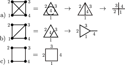
Figure 2: Integrals of intersection diagrams are approximated by consecutive contraction of their intersection centers. The example shows the three 4-particle Mayer clusters, their dual intersection diagrams, and their allowed contractions defined by the Mayer clusters.

as shown in Fig. 2 for the four particle cluster diagrams.

Intersection diagrams can be classified by their number of intersection centers $h$ and internal loops $g$. Taking this into account, the excess free-energy functional density is the infinite sum

$$\Phi=\sum_{g=0,h=1}^{\infty}\Phi_{g,h}\;,$$ (2)

where each element $\Phi_{g,h}$ corresponds itself to an infinite set of diagrams.

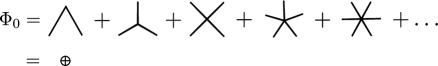
Figure 3: The starfish like diagrams follow from the completely connected Mayer clusters by maximally contraction of their intersection centers. Resummation of all these diagrams is indicated by the crossed circle which corresponds to the Rosenfeld functional.

The leading element, $\Phi_{0,1}$, is presented in Fig. 3 and provides the graphical representation of Rosenfeld’s functional as the intersection probability of the universal stack. Observe that similar diagrams have been used in schmidt-diagram to relate the virial expansion to FMT.

The intersection probability for each stack $\text{St}_{k}$ is determined by the Euler form $K(\partial\text{St}_{k})$, integrated over the intersection domain $\vec{r}_{a}\in\text{St}_{k}$ and averaged over the positions and rotations of each individual particle

$$\begin{split}\Gamma(D):=\{\,\gamma=(\vec{r}&,\vec{\Omega})\,|\,\vec{r}\in D,\,\vec{\Omega}\in\text{SO}(3)\,\}\\[3.99994pt] d\gamma_{i}&:=d^{3}r_{i}\,d^{3}\Omega_{i}\;.\end{split}$$ (3)

To keep the notation for the coordinates of particles and their intersection centers apart, their indices will be labeled by the characters:

$$\begin{array}[]{ll}a,b,c,\ldots&\text{: indices of intersection domains}\\ i,\;j,\;k,\;\ldots&\text{: indices of particle domains\;.}\end{array}$$ (4)

Suitably normalized korden-2 and multiplied by the single particle densities $\rho_{i}$, the Euler form determines the virial coefficient at 0-loop order

$$\begin{split}\beta_{k-1}^{(0,1)}&=\frac{1}{4\pi}\int_{\text{St}_{k}\times\Gamma(D_{2}\times\ldots\times D_{k})}K(\partial\text{St}_{k-1})\,\delta(\vec{n}\vec{r}_{a})\,d^{3}r_{a}\\[3.99994pt] &\qquad\quad\times\rho_{1}(\gamma_{1})\ldots\rho_{k}(\gamma_{k})\,d\gamma_{2}\wedge\ldots\wedge d\gamma_{k}\;,\end{split}$$ (5)

taking into account the symmetry factor $\sigma_{k-1}=1$ of the fully connected Mayer diagrams. The delta-function $\delta(\vec{n}\vec{r}_{a})$ of the scalar-product of the normal and position vector restricts the integrand to the surface $\partial D$ and follows the calculational rules introduced in Appendix B of korden-2 .

The Euler form is a linear functional on the boundary of manifolds, which vanishes for any odd-dimensional domain. The derivation of $K(\partial\text{St}_{k})$ for 3-dimensional particles thus reduces to only three contributions. Introducing the surface $\Sigma$ of a domain $D$ and the notations:

$$\Sigma=\partial D\;,\quad\Sigma^{n}=\underbrace{\Sigma\,\cap\,\ldots\,\cap\,\Sigma}_{n-\text{times}}\,,$$ (6)

the boundary of a stack of $k$ identical particles reduces to

$$\begin{split}\partial\text{St}_{k}&=k\,\Sigma\cap\text{St}_{k-1}+k(k-1)\,\Sigma^{2}\cap\text{St}_{k-2}\\ &\quad+k(k-1)(k-2)\,\Sigma^{3}\cap\text{St}_{k-3}\end{split}$$ (7)

as the intersection probability between the set of points $\Sigma^{3}$ and a further surface element $K(\Sigma^{3}\cap\Sigma)=0$ is zero. The only non-vanishing terms of the Euler form are therefore:

$$\begin{split}K(\Sigma)\;\,&=\,\omega_{\chi}\\ K(\Sigma^{2})&=C^{\alpha_{1}\alpha_{2}}\omega_{\alpha_{1}}\omega_{\alpha_{2}}\\ K(\Sigma^{3})&=C^{\alpha_{1}\alpha_{2}\alpha_{3}}\omega_{\alpha_{1}}\omega_{\alpha_{2}}\omega_{\alpha_{3}}\;,\end{split}$$ (8)

with the $C$-matrices $C^{\alpha_{1}\alpha_{2}}$, $C^{\alpha_{1}\alpha_{2}\alpha_{3}}$ explicitly derived in korden-2 . As first shown by Chern chern-2 , these tensors are independent of the particle geometry and solely defined by the Euler form and the dimensions of the particles and their embedding space.

To this list of algebraic relations it is useful to add a further one, which follows from the tensorial density of the integrand (5):

$$K(\Sigma^{n}\cap\text{St}_{k})=K(\Sigma^{n})\,(\omega_{v})^{k}\;.$$ (9)

For 3-dimensional convex particles it has been shown in korden-2 that the infinite dimensional basis set of weight functions can be grouped into five classes:

$$\omega_{\chi}(\vec{r}_{a}-\vec{r}_{i}) =\frac{1}{4\pi}\kappa_{G}\delta(\vec{n}\vec{r}_{a})$$

$$\omega_{\kappa L}(\vec{r}_{a}-\vec{r}_{i}) =\frac{1}{4\pi}\bar{\kappa}\vec{n}^{\otimes L}\delta(\vec{n}\vec{r}_{a})$$

$$\omega_{\Delta L}(\vec{r}_{a}-\vec{r}_{i}) =\frac{1}{4\pi}\Delta\vec{n}^{\otimes L}\delta(\vec{n}\vec{r}_{a})$$ (10)

$$\omega_{\sigma L}(\vec{r}_{a}-\vec{r}_{i}) =\vec{n}^{\otimes L}\delta(\vec{n}\vec{r}_{a})$$

$$\omega_{v}(\vec{r}_{a}-\vec{r}_{i}) =\Theta(\vec{r}_{a}-\vec{r}_{i})\;,$$

corresponding to the Euler-characteristic $\chi$ of the Gauss curvature $\kappa_{G}$, the mean curvature $\bar{\kappa}$, the curvature difference or tangential curvature $\Delta$, the surface $\sigma$, and the particle volume $v$. Each of these geometric terms is taken at the intersection center $\vec{r}_{a}$ with respect to their absolute position in the embedding space $\vec{r}_{i}$. As a consequence of the non-algebraic splitting of the scalar Euler form, the weight functions also depend on the $L$-fold tensor product of the normal vector $\vec{n}$ for $L~{}\in~{}\mathbb{N}_{0}$.

The weight function $\omega_{v}$ of the particle volume $v$ plays a special role. It is not part of the curvature dependent Euler form (8) but constrains the integration domain in (5) from the embedding space $\mathbb{R}^{3}$ to the particle volume. The relation (9) is therefore a formal one. Nonetheless, it is useful to include it to the set of algebraic relations (8) and to introduce two different indices for the weight functions

$$\begin{split}A,B,C\ldots&\in\{v,\chi,\kappa L,\sigma L\}\\ \alpha,\beta,\gamma\ldots&\in\{\chi,\kappa L,\sigma L\}\;,\end{split}$$ (11)

indicating if $v$ is included or not. The characters are chosen such that to each intersection center $\vec{r}_{a}\in\text{St}_{k}$ the family of indices $(a,A_{1},\alpha_{1},A_{2},\alpha_{2},\ldots)$, $(b,B_{1},\beta_{1},\ldots)$, $(c,C_{1},\gamma_{1},\ldots)$, …is assigned, providing an intuitive relation between weight indices and intersection points.

It is a special property of the 0-loop order (5) and its single intersection center that each particle domain $D_{i}$ is related to a single weight function $\omega_{A}^{i}$. Only in this special case, it is possible to combine them into the 1-point density

$$n_{A}(\vec{r}_{a})=\sum_{i=1}^{M}\int_{\Gamma(D_{i})}\rho_{i}(\gamma_{i})\,\omega^{i}_{A}(\vec{r}_{a}-\vec{r}_{i})d\gamma_{i}$$ (12)

introduced by Rosenfeld rosenfeld-structure . Whereas higher loop orders require the definition of the “$k$-point function”

$$\prod_{p=1}^{k}\omega_{A_{p}}^{i}(\vec{r}_{a_{p}}-\vec{r}_{i})$$ (13)

for $k$ disjunct intersection centers $\vec{r}_{a_{p}}$ at particle domain $\vec{r}_{i}\in D_{i}$ and its corresponding “$k$-point density“

$$\begin{split}&n_{A_{1},\ldots,A_{k}}(\vec{r}_{a_{1}},\ldots,\vec{r}_{a_{k}})\\ &\quad=\sum_{i=1}^{M}\int_{\Gamma(D_{i})}\rho_{i}(\gamma_{i})\,\prod_{p=1}^{k}\omega_{A_{p}}^{i}(\vec{r}_{a_{p}}-\vec{r}_{i})\,d\gamma_{i}\;,\end{split}$$ (14)

as introduced in korden-2 , generalizing Eq. (12) and Wertheim’s 2-point measure wertheim-1 ; wertheim-2 ; wertheim-3 ; wertheim-4 .

Due to the coupling of the particle density to the weight functions, the free energy $F$ is no longer a functional of $\rho_{i}$ alone. Instead, $F$ now depends on the new variable $n_{v}$. As has been shown in korden-2 , the weight function $\omega_{v}$ acts as the neutral element under removing $\text{St}_{k}\to\text{St}_{k-1}$ or adding $\text{St}_{k}\to\text{St}_{k+1}$ a particle and thus shifting the Euler form (9) by one factor of $\omega_{v}$. The corresponding shifts for the boundary of the stack (7) or its Euler form

$$\begin{split}K(\partial\text{St}_{k})&=k\,K(\Sigma)\,\omega_{v}^{k-1}+k(k-1)\,K(\Sigma^{2})\,\omega_{v}^{k-2}\\ &\quad+k(k-1)(k-2)\,K(\Sigma^{3})\,\omega_{v}^{k-3}\end{split}$$ (15)

are generated by integration and differentiation with respect to $\omega_{v}$:

$$\begin{split}\int K(\partial\text{St}_{k})\,d\omega_{v}&=\frac{1}{k+1}\,K(\partial\text{St}_{k+1})\\ \frac{\delta K(\partial\text{St}_{k})}{\delta\omega_{v}}&=k\,K(\partial\text{St}_{k-1})\end{split}$$ (16)

and thus relate intersection integrals (5) for more than three particles $k\geq 3$. These operations allow to translate the virial expansion in the particle density representation $\rho$ to that in the weight density $n_{v}$. To see this, consider the virial expansion of the chemical potential mcdonald , written for constant $\rho$ and $\beta^{-1}=\text{k}_{B}T$:

$$\begin{split}\beta_{k-1}&=\frac{1}{V}\frac{\sigma_{k}}{(k-1)!}\int f_{1,2}\ldots f_{k-1,k}\,d\gamma_{1}\ldots d\gamma_{k}\\ &\quad\beta\mu=\beta\mu_{\text{id}}+\sum_{k=2}^{\infty}\beta_{k-1}\rho^{k-1}\;,\end{split}$$ (17)

depending on the embedding volume $V$ and the symmetry coefficient $\sigma_{k}$.

From this derives the free energy potential by adding one further particle, realized as the integral over $\rho$:

$$\begin{split}\beta F&=\beta F_{\text{id}}+\beta F_{\text{ex}}=\int\beta\mu(\rho)\,d\rho\\ &\;\,\beta F_{\text{ex}}=\sum_{k=2}^{\infty}\;\int\frac{1}{k}\;\beta_{k-1}\rho^{k}\;.\end{split}$$ (18)

In the representation of weight densities, the last step corresponds to the shift $\text{St}_{k-1}\to\text{St}_{k}$ in the particle stack, which for $k\geq 3$ particles is realized as the integral over $n_{v}$.

The operations (16) therefore apply to the free energy functional, defined as the generating function of cluster integrals. With the functional derivative

$$\frac{\delta n_{A}(\vec{r}_{a})}{\delta n_{B}(\vec{r}_{b})}=\delta_{AB}\,\delta(\vec{r}_{a}-\vec{r}_{b})\;,$$ (19)

the free energy $F$ is related to the free energy density $\Phi$ by the integral

$$\beta F =\int\frac{\delta(\beta F)}{\delta n_{v}(\vec{r}_{a})}\delta n_{v}(\vec{r}_{a})=\int\frac{\delta(\beta F)}{\delta n_{v}(\vec{r}_{a})}\,dn_{v}(\vec{r}_{a})\,d^{3}r_{a}$$

$$=:\int\Phi(\vec{r}_{a})\,d^{3}r_{a}$$

$$=\sum_{g,h}\int\Phi_{g,h}(\vec{r}_{a_{1}},\ldots\vec{r}_{a_{h}})\,d^{3}r_{a_{1}}\ldots d^{3}r_{a_{h}}\,,$$ (20)

which reduces to the expansion in intersection diagrams by Eq. (2). Comparing this result to the virial representation of the free energy (18) yields a relation between the density functionals $\Phi_{g,h}$ and their corresponding cluster densities

$$\begin{split}\Phi([n_{A}],\vec{r}_{a})&=\int\sum_{k=2}^{\infty}\;\frac{1}{k}\;\beta_{k-1}([n_{A}],\vec{r}_{a})\,dn_{v}\\ &=\int\sum_{k=2}^{\infty}\;\frac{1}{k}\;\sum_{g,h}\;\beta_{k-1}^{(g,h)}([n_{A}],\vec{r}_{a})\,dn_{v}\end{split}$$ (21)

that is uniquely defined up to an integration constant. Its value has been determined in korden-2 and corresponds to the formal definition of a single particle virial coefficient

$$\beta_{0}=\beta_{0}^{(0,1)}:=n_{\chi}\;.$$ (22)

The final step in proving the equivalence of the intersection probability of the universal stack and Rosenfeld’s functional consists in deriving the first element $\Phi_{0,1}$ of (II). Inserting the algebraic representations (8), (9) into the Euler form (15) and rewriting the cluster integral (5) in 1-point densities

$$\frac{1}{k}\beta^{(0,1)}_{k-1}([n_{A}])=\int\Bigl{[}\omega_{\chi}^{i_{1}}(\omega_{v}^{k-1})^{i_{2}\ldots i_{k}}\Bigr{.}$$

$$+(k-1)\,C^{\alpha_{1}\alpha_{2}}\omega_{\alpha_{1}}^{i_{1}}\omega_{\alpha_{2}}^{i_{2}}(\omega_{v}^{k-2})^{i_{3}\ldots i_{k}}$$

$$\Bigl{.}\;+(k-1)(k-2)\,C^{\alpha_{1}\alpha_{2}\alpha_{3}}\omega_{\alpha_{1}}^{i_{1}}\omega_{\alpha_{2}}^{i_{2}}\omega_{\alpha_{3}}^{i_{3}}(\omega_{v}^{k-3})^{i_{4}\ldots i_{k}}\Bigr{]}$$

$$\qquad\times\rho_{i_{1}}\ldots\rho_{i_{k}}\,d\gamma_{i_{2}}\ldots d\gamma_{i_{k}}\,d^{3}r_{a}$$ (23)

$$=\int\Bigl{[}n_{\chi}n_{v}^{k-1}+(k-1)\,C^{\alpha_{1}\alpha_{2}}n_{\alpha_{1}}n_{\alpha_{2}}n_{v}^{k-2}\Bigr{.}$$

$$\quad\Bigl{.}+\,(k-1)(k-2)\,C^{\alpha_{1}\alpha_{2}\alpha_{3}}n_{\alpha_{1}}n_{\alpha_{2}}n_{\alpha_{3}}n_{v}^{k-3}\Bigr{]}\,d^{3}r_{a}$$

yields the decoupled integral for a stack of order $k$. Adding up all cluster integrals and integrating over the packing density $n_{v}$

$$\Phi_{0,1}([n_{A}],\vec{r}_{a})=\int\sum_{k=1}^{\infty}\frac{1}{k}\beta_{k-1}^{(0,1)}([n_{A}],\vec{r}_{a})\,dn_{v}(\vec{r}_{a})$$ (24)

$$=\int\left[\frac{n_{\chi}}{1-n_{v}}+C^{\alpha_{1}\alpha_{2}}\frac{n_{\alpha_{1}}n_{\alpha_{2}}}{(1-n_{v})^{2}}\right.$$

$$\left.\qquad\qquad\qquad+\,2\,C^{\alpha_{1}\alpha_{2}\alpha_{3}}\frac{n_{\alpha_{1}}n_{\alpha_{2}}n_{\alpha_{3}}}{(1-n_{v})^{3}}\;\right]\;dn_{v}(\vec{r}_{a})$$

reproduces Rosenfeld’s functional

$$\Phi_{0,1} =-n_{\chi}\,\ln{(1-n_{v})}$$ (25)

$$\quad+C^{\alpha_{1}\alpha_{2}}\frac{n_{\alpha_{1}}n_{\alpha_{2}}}{1-n_{v}}+C^{\alpha_{1}\alpha_{2}\alpha_{3}}\frac{n_{\alpha_{1}}n_{\alpha_{2}}n_{\alpha_{3}}}{(1-n_{v})^{2}}$$

and identifies it as the 0-loop order of the expansion in intersection centers.

The simple structure of this result is explained by the single intersection point, as shown in Fig. 3. However, higher order intersection diagrams, as shown in Fig. 2, not only incorporate further intersection points but also loop constraints that create corrections to the direct correlation function at distances larger than the particle diameter. Going beyond the Percus-Yevick approximation requires therefore the introduction of additional mathematical tools.

III The intersection algebra

Intersection diagrams were introduced in korden-2 to visualize the approximation scheme of FMT and to associate the virial expansion of the free energy to the Euler form and thus to Rosenfeld’s functional. They also gave a first intuitive understanding of higher order corrections as partially contracted diagrams. Figures Fig. 1 and Fig. 2 demonstrate how they can be obtained by graphical construction. For more complex diagrams, however, this approach becomes unwieldy and algebraic rules for their construction and manipulation are more useful.

As an example, we will first reconsider the intersection diagrams of Fig. 1 and Fig. 2 in detail in the first paragraph III.2 and then generalize the results to diagrams of arbitrary degree of contraction in III.3.

III.1 Intersection diagrams

The Euler form provides a unique identity between Mayer’s $f$ function and the weight functions

$$\begin{split}&f_{ij}(\vec{r}_{i}-\vec{r}_{j})\\ &=\int_{D_{i}\cap D_{j}}C^{A_{1}A_{2}}\omega_{A_{1}}^{i}(\vec{r}_{a}-\vec{r}_{i})\omega_{A_{2}}^{j}(\vec{r}_{a}-\vec{r}_{j})\,d^{3}r_{a}\end{split}$$ (26)

and relates the representation in particle $\vec{r}_{i},\vec{r}_{j}$ and intersection coordinates $\vec{r}_{a}$. Thus any sequence of $f$ functions $f_{12}f_{13}f_{14}\ldots$, multiplied by their particle densities, can uniquely be rewritten in $k$-point densities (14) as a function of their intersection coordinates.

The simplest diagram, apart from the second virial cluster, is the triangle graph, which has been discussed by Wertheim wertheim-1 ; wertheim-2 ; wertheim-3 ; wertheim-4 and in korden-2 . Using the indices of Fig. 4b), its corresponding integral in weight functions

$$\beta_{2} =\frac{1}{2V}\int\;f_{12}f_{23}f_{31}\,\rho_{1}\rho_{2}\rho_{3}\;d\gamma_{1}d\gamma_{2}d\gamma_{3}$$

$$=\frac{1}{2V}\int\;C^{A_{1}A_{2}}\omega^{1}_{A_{1}}(\vec{r}_{a}-\vec{r}_{1})\omega^{2}_{A_{2}}(\vec{r}_{a}-\vec{r}_{2})$$

$$\qquad\quad\times C^{B_{2}B_{3}}\omega^{2}_{B_{2}}(\vec{r}_{b}-\vec{r}_{2})\omega^{3}_{B_{3}}(\vec{r}_{b}-\vec{r}_{3})$$ (27)

$$\qquad\quad\times\;C^{C_{3}C_{1}}\omega^{3}_{C_{3}}(\vec{r}_{c}-\vec{r}_{3})\omega^{1}_{C_{1}}(\vec{r}_{c}-\vec{r}_{1})$$

$$\quad\times d^{3}r_{a}d^{3}r_{b}d^{3}r_{c}\,\rho_{1}(\gamma_{1})\rho_{2}(\gamma_{2})\rho_{3}(\gamma_{3})\;\,d\gamma_{1}d\gamma_{2}d\gamma_{3}$$

is a functional of the particle densities. The same integral in 2-point densities (14) allows the more compact notation

$$\beta_{2}=\frac{1}{2V}C^{A_{1}A_{2}}C^{B_{2}B_{3}}C^{C_{3}C_{1}}$$ (28)

$$\times\int n_{A_{1}C_{1}}(\vec{r}_{ac})n_{A_{2}B_{2}}(\vec{r}_{ab})n_{B_{3}C_{3}}(\vec{r}_{bc})\,d^{3}r_{ab}d^{3}r_{bc}d^{3}r_{ca}$$

using the distance vectors $\vec{r}_{ab}=\vec{r}_{b}-\vec{r}_{a}$.

In the following discussion neither the dependence on the particle densities nor the loop constraints will be of relevance, so that the identity (26) can be written in the simplified form

$$f_{12}(A)\widehat{=}C^{A_{1}A_{2}}\omega_{A_{1}}\omega_{A_{2}}\;,$$ (29)

using the index combination

$$\begin{split}A_{i}\;:\quad&\text{weight index $A$ at intersection}\\ &\text{domain $\vec{r}_{a}$ of particle $i$}\end{split}$$ (30)

and omitting any reference to the integration over the intersection coordinates. The index $A$ has now two meanings. On the one hand it indicates the intersection center $A$, on the other hand it also numbers the link of the Mayer cluster $f_{ij}(A)$, as seen in Fig. 4a).

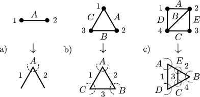
Figure 4: Examples for the index conventions for Mayer and intersection diagrams. For pairwise intersecting particles, the two representations are dual to each other with the role of nodes and edges interchanged. Upper case letters indicate Mayer bonds or intersection centers. Whereas particle numbers represent root points or particle lines.

The two representations (III.1) and (28) of the three particle Mayer cluster of Fig. 4b) can now be written in the more convenient form:

$$f_{12}(A)f_{23}(B)f_{31}(C)$$ (31)

$$\widehat{=}C^{A_{1}A_{2}}\omega_{A_{1}}\omega_{A_{2}}\cdot C^{B_{2}B_{3}}\omega_{B_{2}}\omega_{B_{3}}\cdot C^{C_{3}C_{1}}\omega_{C_{3}}\omega_{C_{1}}$$

$$=C^{A_{1}A_{2}}C^{B_{2}B_{3}}C^{C_{3}C_{1}}(\omega_{A_{1}}\omega_{C_{1}})(\omega_{A_{2}}\omega_{B_{2}})(\omega_{B_{3}}\omega_{C_{3}})$$

with the definition of the 2-point function (13) indicated by parenthesis. Correspondingly, example Fig. 4c) is the product of 3-point and 2-point functions

$$\begin{split}&f_{12}(A)f_{23}(E)f_{34}(C)f_{41}(D)f_{24}(B)\\[3.99994pt] &\widehat{=}C^{A_{1}A_{2}}C^{E_{2}E_{3}}C^{C_{3}C_{4}}C^{D_{1}D_{4}}C^{B_{2}B_{4}}\\[3.99994pt] &\times(\omega_{A_{1}}\omega_{D_{1}})(\omega_{A_{2}}\omega_{B_{2}}\omega_{E_{2}})(\omega_{C_{3}}\omega_{E_{3}})(\omega_{C_{4}}\omega_{B_{4}}\omega_{D_{4}})\;.\end{split}$$ (32)

Comparing the three examples (29), (31), and (32) to their corresponding Mayer diagrams in Fig. 4 reveals a simple building rule for virial integrals represented in weight functions. Define the ”Mayer vertex“ as the node of a Mayer diagram with its attached edges, as shown in Fig. 5a).

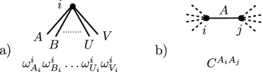
Figure 5: Substitution rules for Mayer diagrams: a) The Mayer vertex of particle $i$ with $k$ attached bonds corresponds to a $k$-point function and b) the Mayer bond linking particles $i$ and $j$ maps to a $C$-matrix.

The cluster integral can then be read off directly from the Mayer graph by the substitution

$$\begin{split}\text{Mayer vertex}&\to\text{$k$-point function}\\ \text{Mayer bond}&\to\text{$C$-matrix}\end{split}$$ (33)

multiplied by the particle densities, loop constraints, integral measures, and the symmetry factor. For the generic case of pairwise intersecting particles, this simple replacement defines a unique mapping between the representation of Mayer and intersection diagrams.

Graphically, the building rule (33) corresponds to an exchange of nodes and edges, as shown in Fig. 4, which in terms of graph theory defines the ”dual graph“ diestel of the Mayer diagram. However, this bijection still provides no simplification of the integral, and the evaluation of the dual diagram is as complicated and unmanageable as it is for the original virial cluster. The next step considers therefore the systematic approximation of intersection diagrams of pairwise intersecting particles.

III.2 Contraction rules

It has already been shown in korden-2 that the structure of intersection diagrams can be simplified by moving some of their intersection centers into a single one. This process of ”contraction“ increases the rotational and translational degrees of freedom over which the statistical system is averaged. It therefore reduces the complexity of the virial integrals but also coarsen their spatial resolution. For the most simplest cases, as the clusters of Fig. 2 and Fig. 3, the contraction of diagrams can be done by hand.

To derive an algebraic set of contraction relations, consider the pairwise contraction of the triangle diagram shown in Fig. 6a).

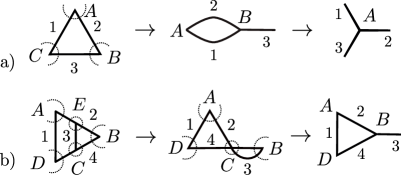
Figure 6: The approximation scheme of FMT is based on the successive contraction of intersection points. Reducible diagrams are intermediate steps with two particles intersecting more than once. Further contractions finally result in irreducible graphs.

The three intersection centers are combined in two steps: First, $C$ is shifted into $B$, leaving the point $A$ invariant; then $B$ is shifted into $A$. For each of the three diagrams of Fig. 6a) we can now write down their corresponding virial integrand, using the splitting rules (8) and (9) of the Euler form:

$$C^{A_{1}A_{2}}\,\omega_{A_{1}}\omega_{A_{2}}\cdot C^{B_{2}B_{3}}C^{C_{3}C_{1}}\,\omega_{B_{2}}\omega_{B_{3}}\omega_{C_{3}}\omega_{C_{1}}$$

$$\xrightarrow{C\to B}C^{A_{1}A_{2}}\,\omega_{A_{1}}\omega_{A_{2}}\cdot C^{B_{2}B_{3}B_{1}}\,\omega_{B_{2}}\omega_{B_{3}}\omega_{B_{1}}$$ (34)

$$\xrightarrow{B\to A}C^{A_{1}A_{2}A_{3}}\,\omega_{A_{1}}\omega_{A_{2}}\omega_{A_{3}}\;.$$ (35)

The first rule of the contraction operation can now be read off from (34) for the fusion of two intersection centers

$$\begin{split}\lim_{C\to B}&C^{B_{2}B_{3}}C^{C_{3}C_{1}}\,\omega_{B_{2}}\omega_{B_{3}}\omega_{C_{3}}\omega_{C_{1}}\\ =\;&C^{B_{2}B_{3}B_{1}}\,\omega_{B_{2}}\omega_{B_{3}}\omega_{B_{1}}\;.\end{split}$$ (36)

More clearly, the effect of the limit $C\to B$ on the weight functions and $C$-matrices can be grouped into two classes. If the objects belong to different particles

$$\begin{split}&\lim_{C\to B}\omega_{C_{3}}=\omega_{B_{3}}\;,\quad\lim_{C\to B}\omega_{B_{2}}\omega_{C_{3}}=\omega_{B_{2}}\omega_{B_{3}}\\ &\lim_{C\to B}C^{C_{3}C_{1}}=C^{B_{3}B_{1}}\\ \end{split}$$ (37)

the indices of the intersection centers are simply renamed. The same operation for identical particle indices

$$\lim_{C\to B}C^{B_{2}B_{3}}C^{C_{3}C_{1}}\,\omega_{B_{3}}\omega_{C_{3}}=C^{B_{2}B_{3}B_{1}}\omega_{B_{3}}$$ (38)

yields a tensorial contraction of the $C$-matrices, aligned with the removal of one weight function. This operation is only defined in the combination of weight functions and $C$-matrices and cannot be split in the way of (37).

Applying these rules to Eq. (34)

$$\begin{split}\lim_{B\to A}&C^{A_{1}A_{2}}C^{B_{2}B_{3}B_{1}}\,\omega_{A_{1}}\omega_{A_{2}}\omega_{B_{2}}\omega_{B_{3}}\omega_{B_{1}}\\ =\;&C^{A_{1}A_{2}A_{3}}\,\omega_{A_{1}}\omega_{A_{2}}\omega_{A_{3}}\end{split}$$ (39)

reproduces the graphically obtained result of (35), provided Eq. (38) is extended to two identical particle indices. This observation is readily generalized to the pairwise contraction of $n-k$ coincident particle indices

$$\lim_{B\to A} C^{A_{1}\ldots A_{k}A_{k+1}\ldots A_{n}}\;C^{B_{k+1}\ldots B_{n}B_{n+1}\ldots B_{m}}$$

$$\times\omega_{A_{k+1}}\ldots\omega_{A_{n}}\;\omega_{B_{k+1}}\ldots\omega_{B_{n}}$$ (40)

$$=\; C^{A_{1}\ldots A_{k+1}\ldots A_{n}\ldots A_{m}}\omega_{A_{k+1}}\ldots\omega_{A_{n}}\;.$$

Thus the successive contraction of intersection centers generates higher rank $C$-matrices. However, from the splitting rules of the Euler form (8) and (9) we know that the maximal rank of a $C$-matrix for 3-dimensional particles is at most 3 and that all further indices necessarily reduce to the index $v$ of the particle volume. It is therefore natural to combine the two equations (8), (9) into one

$$K(\partial\text{St}_{k})=C^{(A_{1}\ldots A_{k})}\omega_{A_{1}}\ldots\omega_{A_{k}}$$ (41)

and to define the generalized $C$-matrix

$$C^{(A_{i_{1}}A_{i_{2}}A_{i_{3}}A_{i_{4}}\ldots A_{i_{k}})}:=C^{(A_{i_{1}}A_{i_{2}}A_{i_{3}}}\,\delta_{v_{i_{4}}}^{A_{i_{4}}}\ldots\delta_{v_{i_{k}}}^{A_{i_{k}})}\;,$$ (42)

where the parenthesis indicate the symmetrization of all particle indices.

As an example, let us expand Eq. (35) in the neutral element $\omega_{v}$ for three identical particles:

$$C^{(A_{1}A_{2}A_{3})}\,\omega_{A_{1}}\omega_{A_{2}}\omega_{A_{3}}$$ (43)

$$=C^{(\chi_{i_{1}}v_{i_{2}}v_{i_{3}})}\,\omega_{\chi_{i_{1}}}\omega_{v_{i_{2}}}\omega_{v_{i_{3}}}+C^{(\alpha_{i_{1}}\alpha_{i_{2}}v_{i_{3}})}\,\omega_{\alpha_{i_{1}}}\omega_{\alpha_{i_{2}}}\omega_{v_{i_{3}}}$$

$$\quad+C^{(\alpha_{i_{1}}\alpha_{i_{2}}\alpha_{i_{3}})}\,\omega_{\alpha_{i_{1}}}\omega_{\alpha_{i_{2}}}\omega_{\alpha_{i_{3}}}$$

$$=3\,\omega_{\chi}\omega_{v}^{2}+6\,C^{\alpha_{1}\alpha_{2}}\,\omega_{\alpha_{1}}\omega_{\alpha_{2}}\omega_{v}+6\,C^{\alpha_{1}\alpha_{2}\alpha_{3}}\,\omega_{\alpha_{1}}\omega_{\alpha_{2}}\omega_{\alpha_{3}}\;.$$

The result correctly reproduces the Euler form (15) for $k=3$.

The successive application of pairwise contractions on dual Mayer clusters generates a vast number of diagrams. However, some of them correspond to networks with multiple intersections between particles, as shown in Fig. 6a). The first step $C\to B$ generates an intermediate diagram with the particles $1$ and $2$ intersecting twice in the centers of $A$ and $B$. But as one intersection point already determines the position and orientation of their particles uniquely, this diagram is no allowed configuration. Whereas the next contraction, $B\to A$, resolves this ambiguity.

Intermediate diagrams are identified as products of $C$-matrices with more than one common particle index. To distinguish these cases from admissible intersection diagrams, we introduce the notation:

$$\begin{split}&C^{A_{1}\ldots A_{k}A_{k+1}\ldots A_{n}}\;C^{B_{k+1}\ldots B_{n}B_{n+1}\ldots B_{m}}\\ &n-k=1\;:\qquad\text{irreducible intersection}\\ &n-k>1\;:\qquad\text{reducible intersection.}\end{split}$$ (44)

Correspondingly, diagrams without reducible intersections are referred to as ”irreducible diagrams“ and ”reducible diagrams“ otherwise. It follows from their definition that any reducible intersection can be reduced to an irreducible one by further contractions.

Another example is the Mayer diagram of Fig. 4c). Its contractions can be either derived by (III.2) or read off from Fig. 6b)

$$C^{A_{1}A_{2}}C^{B_{2}B_{4}}C^{D_{1}D_{4}}C^{C_{3}C_{4}}C^{E_{2}E_{3}}$$

$$\qquad\times\omega_{A_{1}}\omega_{A_{2}}\omega_{B_{2}}\omega_{B_{4}}\omega_{D_{1}}\omega_{D_{4}}\omega_{C_{3}}\omega_{C_{4}}\omega_{E_{2}}\omega_{E_{3}}$$

$$\xrightarrow{E\to C}C^{A_{1}A_{2}}C^{B_{2}B_{4}}C^{D_{1}D_{4}}C^{C_{2}C_{3}C_{4}}$$ (45)

$$\qquad\times\omega_{A_{1}}\omega_{A_{2}}\omega_{B_{2}}\omega_{B_{4}}\omega_{D_{1}}\omega_{D_{4}}\omega_{C_{2}}\omega_{C_{3}}\omega_{C_{4}}$$

$$\xrightarrow{C\to B}C^{A_{1}A_{2}}C^{D_{1}D_{4}}C^{B_{2}B_{3}B_{4}}$$ (46)

$$\qquad\times\omega_{A_{1}}\omega_{A_{2}}\omega_{D_{1}}\omega_{D_{4}}\omega_{B_{2}}\omega_{B_{3}}\omega_{B_{4}}\;.$$

The first contraction, $E\to C$, yields again an intermediate diagram (45), reducible in the particle numbers $2$ and $4$, which is then transformed into an irreducible one by shifting $C\to B$. The result is the highest possible approximation of the Mayer cluster of Fig. 4c). No further contraction is possible as the particles $1$ and $3$ do not interact directly. This can be seen either from the Mayer diagram, where the corresponding $f_{13}$ is missing, or directly from the intersection diagram of Fig. 6b). Therefore, apart from irreducibility, the intersection diagrams obtained by pairwise contractions also have to be compatible to the bonding relations of its Mayer graph.

Again, compatibility of a diagram can be directly read off from its corresponding Mayer cluster, as each of the generalized $C$-matrices belongs to a completely connected Mayer subdiagram:

$$\begin{split}C^{(A_{1}\ldots A_{k})}\;\widehat{=}\;&\text{completely connected Mayer}\\ &\text{subdiagram of the particles $1,\ldots,k$.}\end{split}$$ (47)

The diagram Fig. 4c) from the previous example can therefore be contracted either to $C^{B_{2}B_{3}B_{4}}$ or $C^{B_{1}B_{2}B_{4}}$, corresponding to their subdiagrams of particle indices $(2,3,4)$ and $(1,2,4)$.

In the next subsection it will be shown that any diagram can be decomposed into its maximally connected subgraphs. In most cases this splitting is uniquely defined. But the current example is one of the exceptional cases, which can be split in at least two different ways, corresponding to a global $\mathbb{Z}_{2}$ symmetry. For such diagrams, it is necessary to count their multiplicity of contractions, indicated by

$$m:\text{contraction multiplicity.}$$ (48)

For the graph of Fig. 4c), the multiplicity is therefore

$$m(1,0,0)=2\quad\text{and}\quad m(n_{1},n_{2},n_{3})=1\quad\text{else.}$$ (49)

III.3 Contraction rules and their algebra

The contraction rules are local mappings on the set of Mayer and intersection diagrams. In order to describe their operations on general graphs, it is practical to introduce a suitable notation for both types of representations.

As only completely connected subdiagrams can be contracted into single intersection centers, they take up the position of prime elements in the set of Mayer clusters and intersection diagrams. Let us therefore introduce the notation:

$$\Gamma_{n}^{\lambda}\;: n$$ completely connected Mayer subdiagram of

particles and external bonds grouped in the

partition $$\lambda$$.

Due to the permutation symmetry of the particle indices of completely connected diagrams, it is sufficient to group the external links into a partition table $\lambda$. For example, $\lambda=[(ABC),(DEFG)]$ assigns the external links $ABC$ to subdiagram $1$ and $DEFG$ to subdiagram $2$.

Any Mayer cluster can now be represented as a product of prime subdiagrams. For example, Fig. 4c) allows the two decompositions:

$$\Gamma_{3}^{(ABD)CE}\,\Gamma_{1}^{CE}=\Gamma_{3}^{(BCE)AD}\,\Gamma_{1}^{AD}\;,$$ (50)

which directly translates to the splitting of the Euler form

$$K(\Gamma_{3}^{(ABD)CE}\,\Gamma_{1}^{CE})=K(\Gamma_{3}^{(ABD)CE})\,K(\Gamma_{1}^{CE})$$ (51)

This notation is far more compact than the representation in weight functions (45), (46).

Analogously, intersection diagrams can be split at each intersection center along their particle lines:

$$\begin{split}\widetilde{\Gamma}_{A}^{\lambda}\;:&\;\text{intersection subdiagram of center $A$ and}\\ &\;\text{partition $\lambda$ of external particle lines.}\end{split}$$ (52)

As an example, the intersection diagram of Fig. 4c) factorizes into the prime elements

$$\widetilde{\Gamma}_{A}^{12}\,\widetilde{\Gamma}_{E}^{23}\,\widetilde{\Gamma}_{B}^{24}\widetilde{\Gamma}_{C}^{34}\,\widetilde{\Gamma}_{D}^{41}\;.$$ (53)

In summary, the derivation and approximation of intersection diagrams reduces to a simple set of operations and constraints. In combination with the splitting rules of the Euler form and its linearity, we now define the ”intersection algebra“:

Definition III.1

Let $K$ be the Euler form and $\Gamma_{n,b}\in\Gamma$ an element of the set of Mayer star-clusters $\Gamma$ with $n$ particles, factorizing into the prime subdiagrams $\Gamma_{m}^{\lambda}$

$$\Gamma_{n}=\prod_{i}\Gamma_{n_{i}}^{\lambda_{i}}\;,\quad n=\sum_{i}n_{i}\;.$$ (54)

The Euler form induces a real, linear operation on the set of Mayer clusters

$$\begin{split}K(x_{1}\Gamma_{n_{1}}+x_{2}\Gamma_{n_{2}})&=x_{1}K(\Gamma_{n_{1}})+x_{2}K(\Gamma_{n_{2}})\\ K(\Gamma_{n})&=\prod_{i}K(\Gamma_{n_{i}}^{\lambda_{i}})\end{split}$$ (55)

for $x_{1},x_{2}\in\mathbb{R}$, defining the ”intersection algebra“ $(K,\Gamma)$. The splitting relation

$$K(\Gamma_{n}^{A})=C^{(A_{1}A_{2}\ldots A_{n})}\,\omega_{A_{1}}\omega_{A_{2}}\ldots\omega_{A_{n}}$$ (56)

induces a representation on $\Gamma$ in weight functions. Intersection centers can be combined by pairwise contractions

$$C:\lambda\to\lambda^{\prime}\;,\quad|\lambda|>|\lambda^{\prime}|\;,$$ (57)

reducing the length of the partition $|\lambda|$ by at least one.

The intersection algebra changes the focus from differential geometry to the representation theory of the symmetric group reps ; sachkov , with the Euler form (56) relating the partition table $\lambda$ of an intersection diagram to the ring of symmetric polynomials. To prove that the contraction operation respects this representation, apply the relation

$$(\sum_{i=0}^{\infty}a_{i}x^{i})(\sum_{j=0}^{\infty}b_{j}x^{j})=\sum_{n=0}^{\infty}(\sum_{k=0}^{n}a_{k}b_{k-n})x^{n}$$ (58)

to the product of two generating functions, contracted in the first particle index $i_{1}$:

$$\lim_{B\to A} (\sum_{n}C^{(A_{1}A_{2}\ldots A_{n})}\omega_{A_{1}}^{i_{1}}\omega_{A_{2}}^{i_{2}}\ldots\omega_{A_{n}}^{i_{n}}\rho_{i_{2}}\ldots\rho_{i_{n}})$$

$$\times(\sum_{k}C^{(B_{1}B_{2}\ldots B_{k})}\omega_{B_{1}}^{i_{1}}\omega_{B_{2}}^{j_{2}}\ldots\omega_{B_{k}}^{j_{k}}\rho_{j_{2}}\ldots\rho_{j_{k}})\;\rho_{i_{1}}$$

$$=\sum_{n}n\,C^{(A_{1}\ldots A_{n})}\omega_{A_{1}}^{i_{1}}\ldots\omega_{A_{n}}^{i_{n}}\rho_{i_{1}}\ldots\rho_{i_{n}}\;,$$ (59)

which again corresponds to the Euler form of a new intersection diagram.

The ring structure of the polynomial (56) greatly simplifies the following derivation of the symmetry factors as well as the construction of vertex functions.

IV Intersection vertices and vertex functions

The mapping (55) uniquely defines the splitting of any intersection diagram into its Euler forms. In principal, this is all one needs to derive higher order corrections of the free energy. However, much of this approach can be simplified by the resummation of subdiagrams. In the following two subsections, the free-energy representation in intersection centers will be generalized. First, it will show in IV.1 that the functional splits locally at each intersection center into vertex functions, whose analytical form will be derived in IV.2

IV.1 The local splitting of the FMT functionals

In the notation of the completely connected intersection diagrams (52), the Rosenfeld functional is representable as the infinite sum

$$\Phi_{0,1}(\vec{r}_{A})=\int\sum_{n=1}^{\infty}\frac{1}{n}K(\widetilde{\Gamma}_{A}^{i_{1},\ldots i_{n}})\,\rho_{i_{1}}\ldots\rho_{i_{n}}\,dn_{v}$$ (60)

over the subclass of diagrams with only one intersection center. An even more concise notation can be obtained using the linearity of the Euler form (55) and considering the weighted sum over diagrams

$$\sum_{n=1}^{\infty}\frac{1}{n}\,\widetilde{\Gamma}_{A}^{(i_{1}\ldots i_{n})}\;,$$ (61)

symmetrizised over the external particle indices. This shortened notation provides a convenient representation for the discussion of diagrammatic resummation.

But the Euler form is only one aspect in the derivation of the free energy. In the following we will also need to generalize the expansion of the functional in intersection centers (II) and to determine their combinatorial prefactors (21) of the virial contributions.

Let us first focus on the expansion of the functional itself. Explicitly written out up to three intersection centers

$$\beta F=\int\left.\frac{\delta(\beta F)}{\delta n_{v}(\vec{r}_{a})}\right|_{g=0}\,\delta n_{v}(\vec{r}_{a})$$

$$+\left.\frac{\delta^{3}(\beta F)}{\delta n_{v}(\vec{r}_{a})\delta n_{v}(\vec{r}_{b})\delta n_{v}(\vec{r}_{c})}\right|_{g=1}\delta n_{v}(\vec{r}_{a})\delta n_{v}(\vec{r}_{b})\delta n_{v}(\vec{r}_{c})$$

$$+\ldots$$

$$=\int\Phi_{0,1}\;d^{3}r_{a}+\Phi_{1,3}\;d^{3}r_{a}d^{3}r_{b}d^{3}r_{c}+\ldots\;,$$ (62)

it reproduces the integral representation of the Rosenfeld functional (24) at first order and yields the next to leading order

$$\begin{split}\Phi_{1,3}=\int\sum_{k=3}^{\infty}\frac{1}{k}&\beta_{k-1}^{(1,3)}(\vec{r}_{a},\vec{r}_{b},\vec{r}_{c})\\ &\times dn_{v}(\vec{r}_{a})dn_{v}(\vec{r}_{b})dn_{v}(\vec{r}_{c})\;,\end{split}$$ (63)

which parallels the structure of (III.1) for $k=3$.

From the local property of the Euler form (55) follows that the virial contribution factorizes into a product of three polynomials, each depending on one of $n_{v}(\vec{r}_{a}),n_{v}(\vec{r}_{b}),n_{v}(\vec{r}_{c})$. Consequently, the integration of (63) factorizes likewise and can be executed for each intersection center individually. The same argument applies of course to all further terms of the expansion (IV.1). The free energy functional decouples into a product of local functionals for each intersection center, coupled only by the loop constraints and the numerical prefactors of the virial integrals.

Given the irregular structure of the symmetry factors $\sigma(\Gamma)$ entering (17) for different diagrams, it is nontrivial that such a splitting of the functionals $\Phi_{g,h}$ should exists. A general proof of this hypothesis would require a classification of the automorphism groups of Mayer clusters under relabeling, which to the best of our knowledge is unknown. We will therefore focus on the leading correction term of the Rosenfeld functional and explicitly derive (63) in the following sections.

The diagrams entering $\Phi_{1,3}$ have three intersection centers grouped into

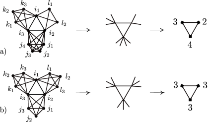
Figure 7: Two examples of the class of triangular diagrams, represented as Mayer graph, maximally contracted intersection diagram, and as weighted graph. Their automorphism groups are: a) $\widetilde{\Gamma}(4,3,2)$: $E_{1}^{3}\times S_{4}\times S_{3}\times S_{2}$ and b) $\widetilde{\Gamma}(3,3,3)$: $G_{12}$.

a ring and thus have a triangular substructure. Two examples are shown in Fig. 7, using the three representations as a Mayer graph, as the maximally contracted intersection diagram, and as a weighted diagram with the number of external lines as index. Using the notation of intersection subdiagrams (52), any such element can be written as

$$\begin{split}\widetilde{\Gamma}(n_{1},n_{2},n_{3})&:=\widetilde{\Gamma}_{A}^{i_{1}i_{2}j_{1}\ldots j_{n_{1}}}\widetilde{\Gamma}_{B}^{i_{2}i_{3}k_{1}\ldots k_{n_{2}}}\widetilde{\Gamma}_{C}^{i_{3}i_{1}l_{1}\ldots l_{n_{3}}}\\ &=(\widetilde{\Gamma}_{A}^{n_{1}})^{i_{1}i_{2}}(\widetilde{\Gamma}_{B}^{n_{2}})^{i_{2}i_{3}}(\widetilde{\Gamma}_{C}^{n_{3}})^{i_{3}i_{1}}\;,\end{split}$$ (64)

with the paired indices $i_{1},i_{2},i_{3}$ defining the backbone of the graph and $j,k,l$ indicating its external lines.

As shown in appendix A, the symmetry factor of a Mayer diagram $\Gamma_{n}$ of $n$ particles is determined by the quotient

$$\sigma(\Gamma_{n})=\frac{|S_{n}|}{|\text{Aut}(\Gamma_{n})|}$$ (65)

of the dimensions of the symmetric group $S_{n}$ and the automorphism group $\text{Aut}(\Gamma_{n})$ of the graph uhlenbeck-ford-1 . This remains true for the dual diagram $\widetilde{\Gamma}$ as the invariance group is independent of the representation of $\Gamma$ and therefore unaffected by contractions

$$\text{Aut}(\Gamma_{n})=\text{Aut}(\widetilde{\Gamma}_{n})\;.$$ (66)

However, our definition of the particle stack (1) and its representation as symmetrized $C$-matrix (42) already includes the invariance group of the completely connected subdiagrams. It is therefore necessary to define an ”effective“ symmetry factor for intersection diagrams $\widetilde{\sigma}(\widetilde{\Gamma}_{n})$ without the invariance group of external particle-lines.

As an example, consider the graph $\widetilde{\Gamma}(3,3,3)$, shown in Fig. 7b). Each of the three intersection centers has $5$ particle-lines attached, of which $2$ are fixed by the triangular backbone diagram, whereas the remaining $3$ external lines are invariant under the permutation $S_{3}$. In order to compensate for the symmetry of the $C$-matrices, the group $S_{3}\times S_{3}\times S_{3}=(S_{3})^{3}$ has to be factored out from $\text{Aut}(\widetilde{\Gamma}(3,3,3))=G_{12}$:

$$G_{12}/(S_{3})^{3}=D_{6}\;.$$ (67)

The quotient group is therefore the automorphism group of the weighted graph shown in Fig. 7b). As demonstrated in appendix A, this result applies to any diagram $\widetilde{\Gamma}(n,n,n)$, independent of the number of external particle-lines.

Generally, it is far easier to derive the reduces invariance group from the weighted diagrams, where the external particle-lines of the intersection graph have been replaced by their number as weight index. Using the results of Tab. 2, the ”reduced automorphism groups“ of triangular diagrams $\widetilde{\Gamma}(n_{1},n_{2},n_{3})$ consists of only four cases:

$$\begin{split}n_{1}\neq n_{2}\neq n_{3}&:\qquad E_{1}^{3}\\ n_{1}=n_{2}\neq n_{3}&:\qquad E_{1}\times\mathbb{Z}_{2}\\ n_{1}=n_{2}=n_{3}&:\qquad D_{6}\\ n_{1}=n_{2}=0,n_{3}=1&:\qquad S_{2}\times\mathbb{Z}_{2}\;,\end{split}$$ (68)

with the exceptional diagram $\widetilde{\Gamma}(1,0,0)$ first discussed in the context of the contraction rules in Sec. III.2.

The reduced invariance group identifies four equivalence classes of diagrams, independent of their particle numbers. This is an important property, as the final goal of determining the free energy functional $\Phi_{1,3}$ requires the resummation of all such diagrams. And here we see that this problem reduces to at most four different classes.

Instead of the symmetry factor for virial integrals (65), $\widetilde{\sigma}$ depends only on the equivalence classes of diagrams and is independent of their particle numbers. In the representation of intersection diagrams (52), the number of external, unpaired particle-lines can be determined from the partition table $\Lambda$:

$$\widetilde{\Gamma}_{n}^{\Lambda}=\prod_{i=1}^{k}\widetilde{\Gamma}_{A_{i}}^{\lambda_{i}}\quad,\quad\Lambda=\{\lambda_{1},\ldots\lambda_{k}\}\;.$$ (69)

Let $(\lambda_{i})_{j}\in\lambda_{i}$ denote an individual element of the partition $\lambda_{i}\in\Lambda$. The set of external lines is then characterized as:

$$\lambda^{\perp}_{i}:=\{\;(\lambda_{i})_{j}\;|\;(\lambda_{i})_{j}\in\lambda_{i}\;,\;(\lambda_{i})_{j}\not\in\lambda_{k}\;,\;\forall\;i\neq k\}\;.$$ (70)

Applied to the triangular diagrams (64), the partition table $\Lambda=(\lambda_{A},\lambda_{B},\lambda_{C})$ consists of the three elements

$$\lambda_{A} =((i_{1},i_{2}),(j_{1},\ldots,j_{n_{1}-2}))\;,$$

$$\lambda_{B} =((i_{2},i_{3}),(k_{1},\ldots,k_{n_{2}-2}))\;,$$ (71)

$$\lambda_{C} =((i_{3},i_{1}),(l_{1},\ldots,l_{n_{3}-2}))\;,$$

from which follows the corresponding orthonormal set of unpaired indices

$$\begin{split}\lambda_{A}^{\perp}=(j_{1},\ldots&,j_{n_{1}-2})\;,\;\lambda_{B}^{\perp}=(k_{1},\ldots,k_{n_{2}-2})\;,\\ \lambda_{C}^{\perp}&=(l_{1},\ldots,l_{n_{3}-2})\;.\end{split}$$ (72)

Using this notation, we define the effective symmetry factor of intersection diagrams:

$$\begin{split}\widetilde{\sigma}(\widetilde{\Gamma}_{n})&:=\frac{1}{n!}\,\sigma(\Gamma_{n})\,\prod_{i}|\lambda_{i}^{\perp}|\,!\\ &\;=\frac{1}{|\text{Aut}(\Gamma_{n})|}\,\prod_{i}|\lambda_{i}^{\perp}|\,!\;,\end{split}$$ (73)

which determines the inverse of the dimension of the reduced invariance group and therefore depends only on their equivalence classes of diagrams. Its values for the triangular diagrams are listed in Tab. 2.

This definition of the symmetry factor not only compensates for the symmetry of the $C$-matrix, but also includes the normalization factor $1/(n-1)!$ of the virial coefficient (17) and the $1/n$ of its integral (18). All numerical prefactors of the free-energy virial expansion are thus included in $\widetilde{\sigma}$.

IV.2 Vertex functions

The new symmetry factor $\widetilde{\sigma}$ does not affect the previous derivation of the Rosenfeld functional (II), (25). Its numerical value for the starfish diagrams with unpaired particle-lines $\lambda_{i}=\lambda_{i}^{\perp}$

$$\widetilde{\sigma}(\widetilde{\Gamma}_{A}^{i_{1}\ldots i_{n}})=\frac{1}{|S_{n}|}\;n!=1$$ (74)

coincides with the corresponding symmetry factor of the Mayer diagram $\sigma(\Gamma_{n}^{A})=1$. The structure of the resummation of 0-loop diagrams (61) remains therefore the same:

$$\begin{split}\sum_{n=1}^{\infty}\frac{\sigma(n)}{n!}\widetilde{\Gamma}_{A}^{i_{1}\ldots i_{n}}&=\sum_{n=1}^{\infty}\frac{\widetilde{\sigma}(n)}{n}\widetilde{\Gamma}_{A}^{(i_{1}\ldots i_{n})}\\ &=\sum_{n=1}^{\infty}\frac{1}{n}\widetilde{\Gamma}_{A}^{(i_{1}\ldots i_{n})}\;.\end{split}$$ (75)

To get a first impression, how this result generalizes to diagrams with more than one intersection center, consider Fig. 8.

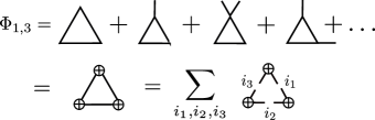
Figure 8: Resummation of the triangular diagrams provides the first order correction to the Rosenfeld functional. With the intersection centers indicated by crossed circles, the functional is the product of three 2-vertex functions summed over the inner particle indices $i_{1},i_{2},i_{3}$.

The first element of the series of triangular diagrams is the exact third virial integral, which later will replace the approximate term in the Rosenfeld functional. The next element is the contracted diagram of $\widetilde{\Gamma}(1,0,0)$, shown in Fig. 2b) and obtained by attaching one additional external particle line to one of the three intersection centers $A,B,C$. Iterating this operation on the backbone diagram, it generates the series of $\Phi_{1,3}$, which can be resummed in the same way as the 0-loop diagrams, shown in Fig. 3. For each intersection center we thus obtain a ”vertex function“ $A\to V_{i_{1}i_{2}}(A)$ depending on the particle-indices $i_{1},i_{2},i_{3}$.

From an algebraic point of view, this factorization of the functional is a consequence of the decomposition of the triangular diagram (64) into subdiagrams. However, although uniquely defined for a given set of particle indices, it is invariant under permutation of the intersection centers $A,B,C$. Instead of the single Mayer graph $\Gamma(1,0,0)$, there exists three identical intersection diagrams:

$$\widetilde{\Gamma}(1,0,0)=\widetilde{\Gamma}_{A}^{2}\widetilde{\Gamma}_{B}^{1}\widetilde{\Gamma}_{C}^{1}=\widetilde{\Gamma}_{A}^{1}\widetilde{\Gamma}_{B}^{2}\widetilde{\Gamma}_{C}^{1}=\widetilde{\Gamma}_{A}^{1}\widetilde{\Gamma}_{B}^{1}\widetilde{\Gamma}_{C}^{2}\;.$$ (76)

In order to compensate for identical products of subdiagrams, let us introduce the

$$p:\text{polynomial multiplicity.}$$ (77)

For the current product of three vertex functions, the combinatorial factor $p(n_{1},n_{2},n_{3})$ for $\widetilde{\Gamma}(n_{1},n_{2},n_{3})$ derives from the binomial coefficient of the generating function:

$$\left(\sum_{n=1}^{\infty}x_{n}\right)^{3}=\sum_{k_{1},k_{2}\ldots=0}^{3}\binom{3}{k_{1},k_{2},k_{3},\ldots}x^{k_{1}}_{1}x^{k_{2}}_{2}x^{k_{3}}_{3}\ldots$$

reducing to the three representative cases of the index-vector $\vec{k}=(k_{1},k_{2},\ldots)$:

$$\begin{split}(1,1,1):\quad n_{1}\neq n_{2}\neq n_{3}&:\quad p=6\\ (2,1,0):\quad n_{1}=n_{2}\neq n_{3}&:\quad p=3\\ (3,0,0):\quad n_{1}=n_{2}=n_{3}&:\quad p=1\end{split}$$ (78)

Taking this into account and the contraction multiplicity $m$ defined in (48), the generating function $\Phi_{1,3}$ reduces to the product of three vertex functions:

$$\Phi_{1,3}(\Gamma)=\sum_{k=0}^{\infty}\,\frac{\sigma(\Gamma_{k+3})}{(k+3)!}\,\Gamma_{k+3}$$ (79)

$$=\sum_{n_{1},n_{2},n_{3}=1}^{\infty}\sum_{i_{1},i_{2},i_{3}}\frac{\sigma(n_{1},n_{2},n_{3})}{(n_{1}+n_{2}+n_{3}+3)!}\,n_{1}!n_{2}!n_{3}!$$ (80)

$$\times\frac{m(n_{1},n_{2},n_{3})}{p(n_{1},n_{2},n_{3})}(\frac{1}{n_{1}!}\widetilde{\Gamma}^{n_{1}}_{A})_{i_{1}i_{2}}(\frac{1}{n_{2}!}\widetilde{\Gamma}^{n_{2}}_{B})_{i_{2}i_{3}}(\frac{1}{n_{3}!}\widetilde{\Gamma}^{n_{3}}_{C})_{i_{3}i_{1}}$$

$$=\widetilde{\kappa}\sum_{i_{1},i_{2},i_{3}}V(A)_{i_{1}i_{2}}V(B)_{i_{2}i_{3}}V(C)_{i_{3}i_{1}}\;,$$ (81)

with the constant $\widetilde{\kappa}$ to be derived in the following.

This result summarizes the central idea of the current work and requires some commends. First, the structure of (79) is uniquely defined by the virial expansion of the free energy (18) and the requirement that its Euler form, suitably multiplied by powers of $\rho$ and integrated over the particle coordinates, yields the free-energy functional density (63). In the next line (80), the representation (64) of the triangular diagrams has been inserted, with only the indices of the backbone diagram $i_{1},i_{2},i_{3}$ explicitely written out. After exchanging the sums in (81), the vertex functions are a convenient abbreviation for the resummed subdiagrams

$$V_{i_{1}i_{2}}(A):=\sum_{n=1}^{\infty}\frac{1}{n!}(\widetilde{\Gamma}_{A}^{n})_{i_{1}i_{2}}\;.$$ (82)

The definition of the vertex function agrees with (61) and introduces the factorials in (80) necessary to replace $\sigma$ by $\widetilde{\sigma}$. The prefactor $\widetilde{\kappa}=\widetilde{\sigma}m/p$ is therefore a function on the equivalence classes of triangular diagrams and can be evaluated by inserting (68), (78), and (49). The detailed calculation can be found in appendix A and yields the overall constant:

$$\widetilde{\kappa}(n_{1},n_{2},n_{3})=\frac{1}{6}\quad\text{for all}\quad\widetilde{\Gamma}(n_{1},n_{2},n_{3})\;,$$ (83)

independent of the particle numbers or equivalence classes. Instead, the prefactor corresponds to its coefficient of the backbone diagram $\widetilde{\kappa}(0,0,0)$.

The splitting of intersection diagrams into subdiagrams restricts the possible dependence of $\widetilde{\kappa}$ on the number of external particle-lines. Because of the invariance of the intersection centers under permutations, the prefactor is either a function of the sum of particle numbers $f(n_{1}+n_{2}+n_{3})$, its product $g(n_{1})g(n_{2})g(n_{3})$ or the product of both. For a general diagram, whose backbone diagram of pairwise intersecting particles has $k$ intersection centers $\widetilde{\Gamma}(n_{1},\ldots,n_{k})$, this generalizes to functions invariant under the automorphism group

$$\widetilde{\kappa}(n_{1},\ldots,n_{k}):\;g\widetilde{\kappa}=\widetilde{\kappa}\;\;\text{for}\;\;g\in\text{Aut}(\widetilde{\Gamma}(0,\ldots,0))\;,$$ (84)

with $\widetilde{\Gamma}(0,\ldots,0)$ as the intersection diagram with all external particle-lines removed. This indicates, but not proves, that the free-energy contribution for a given backbone diagram can be represented by vertex functions that only depend on the number of paired particle-lines. The prefactor for all diagrams coincide and correspond to $\widetilde{\Gamma}(0,\ldots,0)$.

Translating back the diagrammatic representation (82) of the vertex function to the density dependent functional, we define the ”vertex function“ of $k$ internal particle lines

$$V^{i_{1}\ldots i_{n}}(\vec{r}_{a})$$ (85)

$$=\int\sum_{m=0}^{\infty}\frac{1}{m+n}K(\widetilde{\Gamma}_{A}^{(i_{1}\ldots i_{n}k_{1}\ldots k_{m})})\,\rho_{k_{1}}\ldots\rho_{k_{m}}\,dn_{v}$$

as the sum of Euler forms over prime subdiagrams. Here we also used the observation of (IV.1) that the integration over $n_{v}$ factorizes for each intersection center.

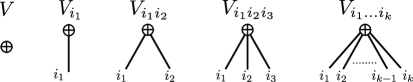
Figure 9: Graphical illustration of $k$-vertex functions: The crossed circle represents the resummation of external, unpaired particle-lines located at a single intersection center. Whereas the outgoing lines correspond to internal particle-lines of the backbone diagram, each carrying one of the $k$ particle indices.

Each $k$-vertex corresponds to a resummed intersection center, indicated by a crossed circle in Fig. 9, and $k$ internal particle-lines.

In terms of vertex functions, the Rosenfeld functional is written as the $0$-vertex

$$\beta F_{0,1}=\int V(\vec{r}_{a})\,d^{3}r_{a}\;,$$ (86)

whereas the Euler form of (79) translates into the product of $2$-vertices

$$\begin{split}\phi_{1,3}(\vec{r}_{a},\vec{r}_{b},\vec{r}_{c})&:=\frac{1}{6}\int V^{i_{1}i_{2}}(\vec{r}_{a})V^{i_{2}i_{3}}(\vec{r}_{b})V^{i_{3}i_{1}}(\vec{r}_{c})\\ &\qquad\quad\times\rho_{i_{1}}\rho_{i_{2}}\rho_{i_{3}}\,d\gamma_{i_{1}}d\gamma_{i_{2}}d\gamma_{i_{3}}\,.\end{split}$$ (87)

Vertex functions are the building blocks of FMT functionals and, in analogy to the derivation of the 0-loop order (25), can be written as a function of $n_{v}$. Setting $k=0$, Eq. (85) reproduces the Rosenfeld functional:

$$V(\vec{r}_{a})=\int\sum_{k=1}^{\infty}\frac{1}{k}K(\widetilde{\Gamma}^{(i_{1}\ldots i_{k})}_{A})\rho_{i_{1}}\ldots\rho_{i_{k}}\,dn_{v}$$

$$=\int\sum_{k=1}^{\infty}n_{\chi}(n_{v})^{k-1}+(k-1)\,C^{\alpha_{1}\alpha_{2}}n_{\alpha_{1}}n_{\alpha_{2}}n_{v}^{k-2}$$

$$\quad+(k-1)(k-2)\,C^{\alpha_{1}\alpha_{2}\alpha_{3}}n_{\alpha_{1}}n_{\alpha_{2}}n_{\alpha_{3}}n_{v}^{k-3}\,dn_{v}$$ (88)

$$=\int n_{\chi}\frac{1}{1-n_{v}}+C^{\alpha_{1}\alpha_{2}}n_{\alpha_{1}}n_{\alpha_{2}}\frac{1}{(1-n_{v})^{2}}$$

$$\quad+2\,C^{\alpha_{1}\alpha_{2}\alpha_{3}}n_{\alpha_{1}}n_{\alpha_{2}}n_{\alpha_{3}}\frac{1}{(1-n_{v})^{3}}\,dn_{v}\;,$$

which yields the $0$-vertex function:

$$V(\vec{r}_{a}) =-n_{\chi}\ln{(1-n_{v})}+C^{\alpha_{1}\alpha_{2}}n_{\alpha_{1}}n_{\alpha_{2}}\frac{1}{1-n_{v}}$$

$$\quad+C^{\alpha_{1}\alpha_{2}\alpha_{3}}n_{\alpha_{1}}n_{\alpha_{2}}n_{\alpha_{3}}\frac{1}{(1-n_{v})^{2}}\;.$$ (89)

Correspondingly, the 1-vertex is a function with a single internal particle-line. However, as the virial expansion of the free-energy of hard particles only depends on star-graphs, no such term will occur. Nonetheless, the 1-vertex provides the first correction in the Mayer expansion of soft potentials with a hard-body center. We will therefore note its form for completeness:

$$V^{i_{1}}(\vec{r}_{a}) =-\omega^{i_{1}}_{\chi}\ln{(1-n_{v})}+C^{\alpha_{1}\alpha_{2}}\omega^{i_{1}}_{\alpha_{1}}n_{\alpha_{2}}\frac{1}{1-n_{v}}$$

$$\quad+C^{\alpha_{1}\alpha_{2}\alpha_{3}}\omega^{i_{1}}_{\alpha_{1}}n_{\alpha_{2}}n_{\alpha_{3}}\frac{1}{(1-n_{v})^{2}}\;.$$ (90)

The analogous calculation with two fixed particle-lines and $\rho_{i_{1}}$, $\rho_{i_{2}}$ removed

$$V^{i_{1}i_{2}}(\vec{r}_{a})=\int\sum_{k=2}^{\infty}\frac{1}{k}K(\widetilde{\Gamma}^{(i_{1}\ldots i_{k})}_{A})\rho_{i_{3}}\ldots\rho_{i_{k}}\,dn_{v}$$

$$=\int\sum_{k=2}^{\infty}(k-1)\,C^{A_{1}A_{2}}\omega_{A_{1}}^{i_{1}}\omega_{A_{2}}^{i_{2}}n_{v}^{k-2}$$

$$\quad+(k-1)(k-2)\,C^{\alpha_{1}\alpha_{2}\alpha_{3}}\omega_{\alpha_{1}}^{i_{1}}\omega_{\alpha_{2}}^{i_{2}}n_{\alpha_{3}}n_{v}^{k-3}\,dn_{v}$$ (91)

$$=\int C^{A_{1}A_{2}}\omega_{A_{1}}^{i_{1}}\omega_{A_{2}}^{i_{2}}\frac{1}{(1-n_{v})^{2}}$$

$$\quad+2\,C^{\alpha_{1}\alpha_{2}\alpha_{3}}\omega_{\alpha_{1}}^{i_{1}}\omega_{\alpha_{2}}^{i_{2}}n_{\alpha_{3}}\frac{1}{(1-n_{v})^{3}}\,dn_{v}$$

yields the $2$-vertex function

$$\begin{split}V^{i_{1}i_{2}}(\vec{r}_{a})&=C^{A_{1}A_{2}}\omega_{A_{1}}^{i_{1}}\omega_{A_{2}}^{i_{2}}\frac{1}{1-n_{v}}\\ &\quad+C^{\alpha_{1}\alpha_{2}\alpha_{3}}\omega_{\alpha_{1}}^{i_{1}}\omega_{\alpha_{2}}^{i_{2}}n_{\alpha_{3}}\frac{1}{(1-n_{v})^{2}}\;.\end{split}$$ (92)

For vertices with more than two particle-lines, the sum reduces to one term only

$$V^{i_{1}\ldots i_{n}}(\vec{r}_{a})=\int\sum_{k=n}^{\infty}\frac{1}{k}K(\widetilde{\Gamma}^{(i_{1}\ldots i_{k})}_{A})\rho_{i_{n+1}}\ldots\rho_{i_{k}}\,dn_{v}$$

$$=\int\sum_{k=n}^{\infty}(n-1)!\binom{k-1}{n-1}C^{A_{1}A_{2}A_{3}}$$

$$\qquad\times\omega_{A_{1}}^{(i_{1}}\omega_{A_{2}}^{i_{2}}\omega_{A_{3}}^{i_{3}}\omega_{v}^{i_{4}}\ldots\omega_{v}^{i_{n})}n_{v}^{k-n}\,dn_{v}$$ (93)

$$=\int(n-1)!\,C^{A_{1}A_{2}A_{3}}$$

$$\qquad\times\omega_{A_{1}}^{(i_{1}}\omega_{A_{2}}^{i_{2}}\omega_{A_{3}}^{i_{3}}\omega_{v}^{i_{4}}\ldots\omega_{v}^{i_{n})}\frac{1}{(1-n_{v})^{n}}\,dn_{v}\;,$$

whose integration yields the vertex function

$$V^{i_{1}\ldots i_{n}}(\vec{r}_{a})=(n-2)!\,C^{A_{1}A_{2}A_{3}}$$ (94)

$$\times\omega_{A_{1}}^{(i_{1}}\omega_{A_{2}}^{i_{2}}\omega_{A_{3}}^{i_{3}}\omega_{v}^{i_{4}}\ldots\omega_{v}^{i_{n})}\frac{1}{(1-n_{v})^{n-1}}\quad\text{for}\;n\geq 3\;,$$

symmetrizised in the particle indices $i_{1},\ldots,i_{n}$.

An important result of the resummation process is the pole structure of the generating functions. The vertex with $k\geq 2$ particle lines has a pole at least of order $k-1$ at packing fraction $n_{v}=1$. This shows that the influence of diagrams rapidly decreases with their number of intersection centers. For the free-energy functional of hard spheres, this explains the success of the Rosenfeld functional. The leading correction $\phi_{1,3}$ will then be of order $-3$ and only take affect at high densities or strong angular correlations between particles, i.e. the solid state of the statistical system.

V The subtraction scheme and first order correction

Using the representation of vertex functions simplifies the derivation of new functionals $\Phi_{g,h}$ for a given backbone diagram. However, as each order of the expansion approximates an infinite subset of Mayer diagrams, it is not possible to simply add its contributions. For example, the Rosenfeld functional $\Phi_{0,1}$ approximates the third virial contribution by its contracted form, whereas $\Phi_{1,3}$ contains its exact integral. The naive sum of both term $\Phi_{0,1}+\Phi_{1,3}$ therefore causes a double counting of diagrams. How to compensate such terms by subtraction will be shown in V.1, followed by the resummation of Mayer ring diagrams and subsequent comparison with the White Bear II functional in V.2.

V.1 The first order correction to Rosenfeld’s functional

The splitting of intersection diagrams into subdiagrams and their subsequent resummation is a local mapping, reflected in vertex functions that each depend on one intersection center only. Thus the global information about the topology of the original Mayer diagram is partially lost. Taking Fig. 7 as an example, the root points of different subdiagrams, indicated by $i,j,k$, are statistically independent, and their Euler form has thus to vanish for concurrent intersection centers. This, however, is in contrast to the functional (87), which is none-zero in the limit of coincident intersection centers $B,C\to A$.

In order to obtain a physically consistent result, the degenerate contribution for $\vec{r}_{a}=\vec{r}_{b}=\vec{r}_{c}$ has to be removed from the integral:

$$\beta F_{1,3}=\int \left[\phi_{1,3}(\vec{r}_{a},\vec{r}_{b},\vec{r}_{c})-\lim_{B,C\to A}\phi_{1,3}(\vec{r}_{a},\vec{r}_{b},\vec{r}_{c})\right]$$

$$\quad\times d\gamma_{a}d\gamma_{b}d\gamma_{c}$$ (95)

The subtraction of the degenerate part from the functional solves two problems: First, it removes the contractions incompatible with the Mayer diagrams. But, as a second effect, it also removes the free-energy contributions of lower diagrammatic orders, that correspond to identical Mayer clusters, but at different order of approximation. For example, the leading term of $\phi_{1,3}(\vec{r}_{a},\vec{r}_{b},\vec{r}_{c})$ is the exact third virial integral, whereas the 3-particle contribution of the Rosenfeld functional $F_{0,1}$ contains only its approximated form as a contracted diagram. Subtracting the contracted diagrams in (V.1) removes therefore its corresponding term in the 0-loop order of $F_{0,1}+F_{1,3}$.

Removing unphysical terms from the free-energy is a common step in the regularization of loop integrals in quantum field theory. Because of this formal resemblance, we will call the current subtraction scheme the ”regularization“ of intersection diagrams.

Using the intersection algebra and the contraction rules for weight functions, the consistency of (V.1) under regularization can be shown explicitly. Leaving out the particle densities in (87), the contraction of the leading contribution of the 2-vertex product

$$\frac{1}{6}\frac{(C^{A_{1}A_{2}}\omega_{A_{1}}\omega_{A_{2}})^{3}}{(1-n_{v})^{3}}=\frac{1}{6}(C^{A_{1}A_{2}}\omega_{A_{1}}\omega_{A_{2}})^{3}+\ldots$$

$$\simeq\frac{1}{6}C^{(A_{1}A_{2}A_{3})}\omega_{A_{1}}\omega_{A_{2}}\omega_{A_{3}}=\frac{3}{6}C^{\chi vv}\omega_{\chi}\omega_{v}^{2}$$ (96)

$$\quad+\frac{3\cdot 2}{6}C^{\alpha_{1}\alpha_{2}}\omega_{\alpha_{1}}\omega_{\alpha_{2}}\omega_{v}+\frac{3!}{6}C^{\alpha_{1}\alpha_{2}\alpha_{3}}\omega_{\alpha_{1}}\omega_{\alpha_{2}}\omega_{\alpha_{3}}$$

$$=\frac{1}{2}\omega_{\chi}\omega_{v}^{2}+C^{\alpha_{1}\alpha_{2}}\omega_{\alpha_{1}}\omega_{\alpha_{2}}\omega_{v}+C^{\alpha_{1}\alpha_{2}\alpha_{3}}\omega_{\alpha_{1}}\omega_{\alpha_{2}}\omega_{\alpha_{3}}$$

reproduces the contracted 3-particle virial and cancels its corresponding part in (25). In summary, the functional

$$F_{\text{K}}=F_{0,1}+F_{1,3}$$ (97)

is exact up to the third virial order and approximates all triangular and completely connected Mayer diagrams. The explicit dependence on 2-point densities now resolves the artificial degeneracy of $F_{0,1}$ in the orientational degrees of freedom. Furthermore, the triangular diagrams describe distance correlations beyond the hard-particle diameter and therefore exceed the Percus-Yevick approximation.

V.2 Approximations and the White Bear functional

With the given set of rules, the derivation of functional corrections of arbitrary order becomes possible. But, as is often the case, including higher order terms does not guarantee higher orders of precision. Possible reasons are the divergence of series and the increasing calculational efforts to evaluate higher order terms. Actually, the benefit of the Rosenfeld functional and the vertex functions is their growing order in $1/(1-n_{v})$, which ensures a fast converging expansion away from its singularity. More restrictive is therefore the second aspect, how to evaluate and minimize higher order terms, whose three and more intersection centers define non-local functionals.

The mathematical framework necessary to evaluate such ring diagrams has been developed by Wertheim and applied to the third virial integral for ellipsoidal geometries at constant particle density wertheim-1 ; wertheim-2 ; wertheim-3 ; wertheim-4 . In the explored range of aspect ration $L\leq 10$, Wertheim found excellent agreement with results of computer simulations.

The same mathematical methods apply to the functional (97), with the tensorial products of the normal vectors in (II) represented by spherical harmonic functions and the convolute of weight functions decoupled by a Radon transformation. The latter reduces to a Fourier transformation in the case of coinciding intersection centers. The subtracted part of (V.1) can therefore be evaluated in the same way as the Rosenfeld functional. Nonetheless, evaluating and minimizing the functional is still a complicated mathematical problem, wherefore the development of efficient approximation strategies will be an important future goal.

One possible ansatz is the improvement of the analytical form of the $n_{v}$-dependence of the functional. The previous results for the 0-loop order and the vertex functions suggest an expansion in powers of $1/(1-n_{v})$. This, however, is a result of the chosen resummation strategy. It is important to observe that different selections of diagrams will also yield a different analytical structure in $n_{v}$. As has been discussed in korden-2 , what marks the vertex functions as special is their possibility to combine with any alternative resummation scheme because of the factorization of Mayer diagrams into completely connected subdiagrams.

In order to improve the $n_{v}$-dependence of the 0-loop order, it is necessary to go beyond the starfish graphs. The first choice is therefore the set of 1-loop diagrams

$$\Phi_{1}=\sum_{h=3}^{\infty}\Phi_{1,h}\;.$$ (98)

As a further approximation we restrict the functionals $\Phi_{g,h}$ to their backbone diagrams, which results in the series shown in the first line of Fig. 10.

Figure 10: $\Phi_{1}$ is the generating functional for all 1-loop Mayer diagrams, whose contraction provides a first order approximation in $n_{v}$ to the Rosenfeld functional.

The functional $\Phi_{1}$ for Mayer ring-diagrams has already been derived in korden-2 as the generating function of Mayer bonds $f_{i_{1}i_{2}}$, written in the matrix notation

$$M_{i_{1}i_{2}}:=C^{A_{1}A_{2}}\omega_{A_{1}}^{i_{1}}\omega_{A_{2}}^{i_{2}}\rho_{i_{1}}\;.$$ (99)

Together with the symmetry factor $\sigma(k)=1/(2k)$ for a ring of $k$ particles, the sum can be rewritten in closed form

$$\Phi_{1}(M) =\sum_{k=3}^{\infty}\;\frac{1}{2k}\;M_{i_{1}i_{2}}M_{i_{2}i_{3}}\ldots M_{i_{k}i_{1}}$$ (100)

$$=-\frac{1}{2}\ln{(1-M)}-\frac{1}{2}M_{i_{1}i_{1}}-\frac{1}{4}M_{i_{1}i_{2}}M_{i_{2}i_{1}}$$

with a logarithmic singularity at $M=1$. It is tempting to assume that this divergency corrects the pole $n_{v}=1$ of highest packing fraction of the 0-loop functional to a physically realistic value that depends on the geometry of the particles. However, minimizing $\Phi_{1}$ will be even more ambitious than that of $F_{\text{K}}$.

As we are only interested in the $n_{v}$-corrections of the Rosenfeld functional, it is sufficient to contract (100) to one intersection center. Using the notation

$$\Gamma_{i_{1}i_{2}\ldots i_{k}}:=<\Gamma_{i_{1}i_{2}}\Gamma_{i_{2}i_{3}}\ldots\Gamma_{i_{k}i_{1}}>$$ (101)

to indicate the contraction of a Mayer diagram, the logarithmic part of (100) can be expanded in orders of $n_{v}$:

$$-\frac{1}{2}<\ln{(1-M)}>=\sum_{k=1}^{\infty}\;\frac{1}{2k}<M^{k}>$$

$$=\int\sum_{k=1}^{\infty}\;\frac{1}{2k}\;K(\frac{1}{k}\Gamma_{i_{1}\ldots i_{k}})\rho^{k}\,dn_{v}$$

$$=\int\sum_{k=1}^{\infty}\;\frac{1}{2k}C^{(A_{1}\ldots A_{k})}n_{A_{1}}\ldots n_{A_{k}}\int_{0}^{1}t^{k-1}d(tn_{v})$$ (102)

$$=\frac{1}{2}\int\frac{n_{\chi}}{1-tn_{v}}+C^{\alpha_{1}\alpha_{2}}n_{\alpha_{1}}n_{\alpha_{2}}\frac{t}{(1-tn_{v})^{2}}$$

$$\quad+2\,C^{\alpha_{1}\alpha_{2}\alpha_{3}}n_{\alpha_{1}}n_{\alpha_{2}}n_{\alpha_{3}}\frac{t^{2}}{(1-tn_{v})^{3}}\,d(tn_{v})\;,$$

where the integration over the scaling parameter $\rho\to t\rho$ absorbs one factor of $1/k$. Evaluating the integral yields the logarithmic contribution

$$-\frac{1}{2}<\ln{(1-M)}>=-\frac{1}{2}n_{\chi}\ln{(1-n_{v})}$$ (103)

$$+C^{\alpha_{1}\alpha_{2}}n_{\alpha_{1}}n_{\alpha_{2}}\frac{1}{4n_{v}(1-n_{v})}[2(1-n_{v})\ln{(1-n_{v})}+2n_{v}]$$

$$-C^{\alpha_{1}\alpha_{2}\alpha_{3}}n_{\alpha_{1}}n_{\alpha_{2}}n_{\alpha_{3}}$$

$$\quad\times\frac{1}{2n_{v}^{2}(1-n_{v})^{2}}[2(1-n_{v})^{2}\ln{(1-n_{v})}+2n_{v}-3n_{v}^{2}]\;.$$

The remaining two terms of (100) are the traces of $M$ and $M^{2}$, which are functions of one intersection center only. Thus, using the subtraction scheme introduced in the last paragraph, both contributions would vanish after regularizing the 1-loop diagrams. Unfortunately, this mechanism does not apply for the current approximation and a better understanding of these two terms is necessary.

Deriving the trace of the contracted form of $M$

$$\begin{split}<M_{i_{1}i_{1}}>&=<C^{A_{1}A_{2}}\omega_{A_{1}}^{i_{1}}\omega_{A_{2}}^{i_{2}}>\rho_{i_{1}}\\ &=<C^{A}\omega_{A}^{i_{1}}>\rho_{i_{1}}=C^{\chi}\omega_{\chi}^{i_{1}}\rho_{i_{1}}=n_{\chi}\end{split}$$ (104)

yields the weight density of the Euler characteristic. It therefore removes in (100) the case of only one intersecting particle. This geometric interpretation is consistent with Fig. 10, where at least three particles have to interact at one intersection point. Generalizing this observation to the calculation (102), we have to subtract the contributions of $K(\Sigma\cap D^{k-1})$ from its sum. The derivation is analogous to the calculation of the 1-vertex (IV.2), only with the symmetry factor replaced by $\sigma(1)=1/2$ and the sum restricted to $\Sigma\cap D^{k-1}$:

$$-\frac{1}{2}\int\sum_{k=1}^{\infty}C^{\chi v\ldots v}n_{\chi}n_{v}^{k-1}\,dn_{v}=\frac{1}{2}n_{\chi}\ln{(1-n_{v})}$$ (105)

The calculation for the second term $M^{2}$ is similar but allows two possible contractions:

$$<M_{i_{1}i_{2}} M_{i_{2}i_{1}}>$$

$$=<C^{A_{1}A_{2}}\omega_{A_{1}}^{i_{1}}\omega_{A_{2}}^{i_{2}}C^{A_{2}A_{1}}\omega_{A_{2}}^{i_{2}}\omega_{A_{1}}^{i_{1}}>\rho_{i_{1}}\rho_{i_{2}}$$

$$=C^{\alpha_{1}\alpha_{2}}n_{\alpha_{1}}n_{\alpha_{2}}$$

$$<M_{i_{1}i_{3}} M_{i_{3}i_{2}}>\rho_{i_{3}}$$ (106)

$$=<C^{A_{1}A_{3}}\omega_{A_{1}}^{i_{1}}\omega_{A_{3}}^{i_{3}}C^{A_{3}A_{2}}\omega_{A_{3}}^{i_{3}}\omega_{A_{2}}^{i_{2}}>\rho_{i_{1}}\rho_{i_{2}}\rho_{i_{3}}$$

$$=C^{\alpha_{1}\alpha_{3}\alpha_{2}}n_{\alpha_{1}}n_{\alpha_{3}}n_{\alpha_{2}}\;,$$

corresponding to intersections of $\Sigma^{2}$ and $\Sigma^{3}$. But as both contributions derive from the same order in $M$, they necessarily have to follow from the same $C$-matrix. With the symmetry factor $\sigma(2)=1/4$, the terms to be removed from (103) are the Euler forms of $K(\Sigma^{2}\cap D^{k-1})$ and $K(\Sigma^{3}\cap D^{k-1})$ multiplied by the same order of $D^{k-1}$ as in (105). The calculation therefore parallels (92) with $n_{\chi}$ removed:

$$\begin{split}-\frac{1}{4}V^{i_{1}i_{2}}&\rho_{i_{1}}\rho_{i_{2}}n_{v}=-\frac{1}{4}C^{\alpha_{1}\alpha_{2}}n_{\alpha_{1}}n_{\alpha_{2}}\frac{n_{v}}{1-n_{v}}\\ &-\frac{1}{4}C^{\alpha_{1}\alpha_{2}\alpha_{3}}n_{\alpha_{1}}n_{\alpha_{2}}n_{\alpha_{3}}\frac{n_{v}}{(1-n_{v})^{2}}\;.\end{split}$$ (107)

The new functional is the sum of the three contributions (103), (105), (107) and the 0-loop order (25):

$$\begin{split}\Phi&=-n_{\chi}\ln{(1-n_{v})}(1+\phi^{(1)})\\ &+C^{\alpha_{1}\alpha_{2}}n_{\alpha_{1}}n_{\alpha_{2}}\frac{1}{1-n_{v}}(1+\phi^{(2)})\\ &+C^{\alpha_{1}\alpha_{2}\alpha_{3}}n_{\alpha_{1}}n_{\alpha_{2}}n_{\alpha_{3}}\frac{1}{(1-n_{v})^{2}}(1+\phi^{(3)})\end{split}$$ (108)

with the three correction terms:

$$\phi_{\text{K}}^{(1)} =0$$

$$\phi_{\text{K}}^{(2)} =\frac{1}{4n_{v}}(2(1-n_{v})\ln{(1-n_{v})}+2n_{v}-n_{v}^{2})$$ (109)

$$\phi_{\text{K}}^{(3)} =\frac{-1}{2n_{v}^{2}}(2(1-n_{v})^{2}\ln{(1-n_{v})}+2n_{v}-3n_{v}^{2}+\frac{1}{2}n_{v}^{3})\;.$$

In this form, the result can be compared to the White Bear II functional, introduced in white-bear-1 ; white-bear-2 , which combines the Boublik-Mansoori-Carnahan-Starling-Leland equation of state mcsl with the structure of the free energy functional, determined by the scaled-particle differential equation rosenfeld-structure . It is therefore not a purely geometrically motivated approach as Rosenfeld’s FMT, but takes into account the numerically derived virial coefficients up to the eighth’s order, combined in a generating function cs .

The WBII functional is independent of positional correlations and therefore of the same structure as (108) with the corresponding correction terms:

$$\phi_{\text{WB}}^{(1)} =0$$

$$\phi_{\text{WB}}^{(2)} =\frac{1}{3n_{v}}[2(1-n_{v})\ln{(1-n_{v})}+2n_{v}-n_{v}^{2}]$$ (110)

$$\phi_{\text{WB}}^{(3)} =\frac{-1}{3n_{v}^{2}}[2(1-n_{v})^{2}\ln{(1-n_{v})}+2n_{v}-3n_{v}^{2}+2n_{v}^{3}])\;.$$

The terms $\phi_{\text{K}}$, $\phi_{\text{WB}}$ are similar, deviating only in their numerical prefactors and the $n_{v}^{3}$-term of $\phi^{(3)}$. Comparing the curve shapes of $\phi^{(2)}_{\text{K}}$ and $\phi^{(2)}_{\text{WB}}$, we find excellent agreement despite this property. Whereas the different $n_{v}^{3}$-terms of $\phi^{(3)}$ cause a significant change in the curve’s curvature. Nonetheless, it is remarkable that the analytical terms of the infinite sum of Mayer diagrams (103) are in good agreement with their analytical counterparts in the White Bear II functional.

VI Discussion and Conclusion

The current article has shifted the previous perspective of korden-2 from differential geometry to the algebraic rules of the Euler form. It systematically generalizes the FMT functional from Rosenfeld’s 0-loop order to any number of intersection centers and develops several new mathematical tools for the efficient manipulation of weight functions.

It has been shown that Mayer’s star graphs have a uniquely defined dual representation in intersection diagrams. These allow an intuitive picture of the Euler form and its decomposition into weight functions. Using this graphical description, we developed the contraction method as an approximation of the underlying Mayer diagrams.

Removing the external particle-lines from an intersection diagram defines its backbone graph, which corresponds to a unique contribution $\Phi_{g,h}$ in the expansion of the free energy functional. The successive attachment of external particle-lines to its intersection centers provides a resummation process that significantly improves the original virial expansion in particle densities. The resulting vertex functions then replace the Mayer functions as the building blocks of the FMT functional.

Resummation is an essential step in the derivation of the functional as it generates the pole structure $1/(1-n_{v})$ of the packing fraction and yields a generic convergence criterion for the expansion in intersection centers. However, its factorization in vertex functions could not be proven in general. The problem relies in the symmetry factors of the infinite sum of Mayer diagrams. For the exemplary case of triangular graphs it could be shown that such a splitting indeed exists as the free-energy prefactor for all such diagrams agrees.

In the current case of triangular diagrams, we first determined the invariance groups under labeling which define four equivalence classes. Furthermore, taking into account the contraction and polynomial multiplicities of their individual vertex contributions, it could be shown that each triangular diagram contributes the same numerical prefactor. This allowed the simple factorization into fully contracted subdiagrams for any triangular graph. For general diagrams, however, we were only able to show that the prefactors for a given backbone diagram transform under the same automorphism group as the diagram itself. Nevertheless, this is enough to deduce that the resummed free energy functional for any Mayer ring-diagram likewise factorizes, with a common prefactor that only depends on its number of intersection centers. But for more general functional contributions of two and more loops, it would be an important step in our understanding to obtain a general expression for this structure.

The resummation of diagrams also involved the regularization of the functional. This process removes those intersection terms that are either incompatible with the Mayer diagrams or contributions of lower order functionals which are now replaced by terms of lesser approximation. Most terms of the subtraction scheme are of zero measure and thus can be ignored completely. A practical application is the summation over all completely contracted Mayer ring-diagrams. The analytical form reproduces the White Bear II functional to good accuracy. However, it is the subtraction of the irregular parts of first and second order that cause the deviation in $n_{v}^{3}$ that does not match with the White Bear result. If this discrepancy could be clarified it would be possible to derive even higher order corrections and exceed the current precision of numerically obtained functionals.

The White Bear II functional provides only a small correction to the bulk properties of the Rosenfeld functional. This suggests that the improvement of the analytical structure in $n_{v}$ will be less important than the inclusion of terms which resolve the orientational degeneration of the 0-loop order and to go beyond the Percus-Yevick approximation. Both deficits are resolved by the three-center term derived in this article. It will therefore be an important next step to find efficient numerical methods to minimize $F_{\text{K}}$.

The new objects entering this functional are the 2-point densities. Whereas the 1-point functions depend on a single vector field moving over the surface of a particle, the 2-point functions determine the correlation between vector fields at two different particle points. Thus, 1-point functions reproduce the ”classical“ curvature depend information of the particle’s geometry, whereas $k$-point functions define a completely new mathematical class of geometric invariant quantities. Fundamental measure theory introduces therefore new mathematical tools that not only give access to important physical problems of many-particle systems but also might provide new answers to mathematical questions that cannot be covered by single vector fields alone. $k$-point functions interpolate between the manageable but approximate description of geometry as a tangential space and non-local geometric properties as, e.g., the maximal packing density of particles in an embedding space.

The derivation of a FMT functional starting from an infinite class of Mayer graphs, then translated to intersection diagrams, and finally resummed into vertex functions is an inefficient approach. Given the diagrams’ systematic and our first experience with ring graphs, we expect the existence of a simpler formulation that closely resembles a field theory with the vertex functions as its variabels. This would completely replace the dependence on Mayer diagrams and their symmetry factors and provide a better understanding of the nature of FMT.

VII Acknowledgment

Matthias Schmidt is kindly acknowledged for helpful discussions and his infinite patience while preparing this work. The author also wishes to thank André Bardow and Kai Leonhard for supporting this work, as well as Annett Schwarz and Christian Jens for carefully proofreading the manuscript. This work was performed as part of the Cluster of Excellence ”Tailor-Made Fuels from Biomass”, funded by the Excellence Initiative of the German federal and state governments.

APPENDIX A

In the following we will determine the automorphism groups and their characteristic parameters (65), (73), and (83) for the triangular Mayer diagrams $\Gamma(n_{1},n_{2},n_{3})$ of the type shown in Fig. 7. To the best of the authors knowledge, no general classification or systematic construction of these groups is known. We will therefore first derive the groups of the first seven diagrams and then deduce their generalization to all further cases.

To put the formulation on a more formal level, consider any star diagram $\Gamma$ and define a representation $\lambda$ of $\Gamma$ by its labeling in Mayer’s $f$ functions:

$$\lambda\;:\;\Gamma\to\text{prod}(f_{ij})\;.$$ (111)

By definition, any product of $f$ functions is only uniquely defined up to their ordering

$$\begin{split}\pi:=\{f_{ij}=f_{ji},\;&f_{ij}f_{kl}=f_{kl}f_{ij}\}\\[5.0pt] \pi\lambda(\Gamma)&=\lambda(\Gamma)\;.\end{split}$$ (112)

As any labeling of the nodes of a Mayer diagram is admissible, there exists $n!$ possible representations for an $n$-particle diagram, generated by operating with the symmetric group $S_{n}$ on any representation $\lambda$:

$$g\in S_{n}\;:\;g\lambda=\lambda^{\prime}\;.$$ (113)

For a discussion of the symmetric group see e.g. hamermesh . However, not all elements of $S_{n}$ generate a new representation. If the operation of $g$ can be undone by a permutation $\pi$, it leaves the labeling invariant, defining a subgroup of $S_{n}$:

$$\text{Aut}(\Gamma)=\{g\in S_{n}\;|\;g\lambda(\Gamma)=\pi\lambda(\Gamma)\}\;,$$ (114)

so that $\pi^{-1}\circ g=\text{id}$. Clearly, the identity $e\in S_{n}$ is element of $\text{Aut}(\Gamma)$, and if $g_{1},g_{2}\in\text{Aut}(\Gamma)$ so is $g_{1}^{-1},g_{2}^{-1}$ and any product of them.

To simplify the notation, let us replace the $f$ functions by square brackets:

$$f_{ij}\to[ij]\;,$$ (115)

on which the permutation symbols $(1,2,3,\ldots)$ of $S_{n}$ operate by cyclic permutation of particle indices.

As an example, consider the labeling of the diagram $\Gamma(1,1,0)$, as shown in Fig. 11 with its $\mathbb{Z}_{2}$-symmetry $2\leftrightarrow 3$, $4\leftrightarrow 5$:

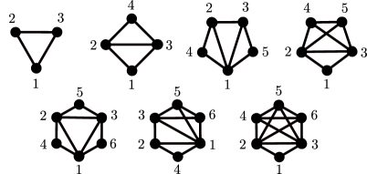
Figure 11: The first Mayer diagrams of up to 6 particles with triangular substructure. $(0,0,0)$, $(1,0,0)$, $(1,1,0)$, $(2,0,0)$, $(1,1,1)$, $(2,1,0)$, and $(3,0,0)$ with the inner triangle defined by the numbers $1\to 2\to 3$.

$$\begin{split}\lambda(\Gamma_{1,1,0})&=f_{12}f_{13}f_{14}f_{15}f_{23}f_{24}f_{35}\\ &=[12][13][14][15][23][24][35]\;.\end{split}$$ (116)

The axial symmetry of the diagram only allows the identity and one further element as the automorphism group

$$\begin{split}(1)(23)(45)&\Bigl{(}[12][13][14][15][23][24][35]\Bigr{)}\\ &\qquad=[13][12][15][14][32][35][24]\end{split}$$ (117)

so that the order of $\text{Aut}(\Gamma(1,1,0))$ is 2.

The graphical representation of the diagrams, shown in Fig. 11, suggests a relation to point-groups. This is of course only true for the simple graphs under consideration, but simplifies the construction of the automorphism groups considerably. For up to six particles, the star diagrams and group elements are as follows:

$$(0,0,0):S_{3}$$ (118)

$$(1)(2)(3),(1)(23),(2)(13),(3)(12),(123),(132)$$

$$(1,0,0):\mathbb{Z}_{2}\times S_{2}$$ (119)

$$(1)(2)(3)(4),(1)(4)(23),(2)(3)(14),(14)(23)$$

$$(1,1,0):E_{1}^{3}\times\mathbb{Z}_{2}$$ (120)

$$(1)(2)(3)(4)(5),(1)(23)(45)$$

$$(2,0,0):E_{1}\times\mathbb{Z}_{2}\times S_{2}$$ (121)

$$(1)(2)(3)(4)(5),(1)(2)(3)(45),(1)(4)(5)(23),$$

$$(1)(23)(45)$$

$$(1,1,1):G_{6}$$ (122)

$$(1)(2)(3)(4)(5)(6),(1)(5)(23)(46),(2)(6)(13)(45),$$

$$(3)(4)(12)(56),(123)(456),(132)(654)$$

$$(2,1,0):E_{1}^{4}\times S_{2}$$ (123)

$$(1)(2)(3)(4)(5)(6),(1)(2)(3)(4)(56)$$

$$(3,0,0):E_{1}\times S_{2}\times S_{3}$$ (124)

$$(1)(2)(3)(4)(5)(6),(1)(2)(3)(4)(56),(1)(2)(3)(5)(46),$$

$$(1)(2)(3)(6)(45),(1)(2)(3)(456),(1)(2)(3)(465),$$

$$(1)(23)(4)(5)(6),(1)(23)(4)(56),(1)(23)(5)(46),$$

$$(1)(23)(6)(45),(1)(23)(456),(1)(23)(465)\;,$$

where $E_{1}$ is the identity element. The diagrams and groups are also listed in Tab. 1.

Table 1: The triangular Mayer diagrams for $n\leq 6$ particles are listed with their automorphism groups and corresponding characteristic numbers: the symmetry factors $\sigma$, $\widetilde{\sigma}$, the polynomial $p$ and contraction multiplicities $m$, and their resulting prefactors $\widetilde{\kappa}$ for the free energy functional.

$\Gamma$	$\text{Aut}(\Gamma)$	$\sigma$	$\widetilde{\sigma}$	$p$	$m$	$\widetilde{\kappa}$
$(0,0,0)$	$S_{3}$	1	1/6	1	1	1/6
$(1,0,0)$	$\mathbb{Z}_{2}\times S_{2}$	6	1/4	3	2	1/6
$(1,1,0)$	$E_{1}^{3}\times\mathbb{Z}_{2}$	60	1/2	3	1	1/6
$(2,0,0)$	$E_{1}\times\mathbb{Z}_{2}\times S_{2}$	30	1/2	3	1	1/6
$(1,1,1)$	$G_{6}$	120	1/6	1	1	1/6
$(2,1,0)$	$E_{1}^{4}\times S_{2}$	360	1	6	1	1/6
$(3,0,0)$	$E_{1}\times S_{2}\times S_{3}$	60	1/2	3	1	1/6

These groups have already been identified by Riddell and published by Uhlenbeck and Ford uhlenbeck-ford-1 . Based on Polya’s counting theorem polya-a ; polya-b , they also developed a counting formula riddell ; uhlenbeck-ford-2 , which determines the number of independent labelings of all Mayer diagrams for a given number of nodes and labels. But a corresponding formula for individual diagrams is still unknown.

For the current case of triangular Mayer diagrams $\Gamma(n_{1},n_{2},n_{3})$, the automorphism groups can be derived from the seven cases (118-124). By comparing their groups with the diagrams of Fig. 11, one observes that the three attached completely connected subdiagrams contribute the symmetric group $S_{n_{1}}\times S_{n_{2}}\times S_{n_{3}}$. For $n_{1}\neq n_{2}\neq n_{3}$, the resulting automorphism group therefore is $E_{1}^{3}\times S_{n_{1}}\times S_{n_{2}}\times S_{n_{3}}$. For $n_{1}=n_{2}\neq n_{3}$, the diagram has an additional axial symmetry $\mathbb{Z}_{2}$, exchanging the two subgroups $S_{n_{1}}\times S_{n_{2}}$. And for $n_{1}=n_{2}=n_{3}$, the symmetry of the backbone diagram extends to the dihedral group $D_{6}$, whose semi-direct product with $S_{n}^{3}$ is denoted as $G_{3n+3}$.

As an example, how to generalize the above seven cases, consider $\Gamma(1,1,1)$ and its extension to $\Gamma(n,n,n)$. In the corresponding diagram of Fig. 11, one replaces the particles $4,5,6$ by a completely connected subdiagram of $n$ particles. The dihedral symmetry of the backbone graph remains unchanged under this operation, so that the group elements (122) can be adjusted by the formal replacement of the particle indices $4,5,6\to A,B,C$ with $A,B,C\in S_{n}$:

$$(n,n,n):G_{3n+3}:$$ (125)

$$(1)(2)(3)(A)(B)(C),\;(1)(23)(B)(AC),(2)(13)(C)(AB),$$

$$(3)(12)(A)(BC),(123)(ABC),\;(132)(CBA)\;.$$

The resulting automorphism group is thus the semi-direct product $D_{6}\rtimes S_{n}^{3}$.

Comparing these invariance groups to Tab. 1, the only diagram that drops out of this classification is $\Gamma(1,0,0)$. Instead of $\mathbb{Z}_{2}\times E_{1}^{2}$, as expected, its automorphism group is $\mathbb{Z}_{2}\times S_{2}$. The reason for this larger group is an additional $\mathbb{Z}_{2}$ symmetry of its diagram, exchanging the two subtriangles $1-2-3$ and $2-3-4$, using the numbering of Fig. 11. As has already been observed in Section III, the contraction of the completely connected subdiagrams is therefore not unique and we have to count the contraction multiplicity $m=2$ for $(1,0,0)$ and $m=1$ for all other triangular diagrams.

Table 2: Complete list of the triangular Mayer diagrams and their automorphism groups, their intersection symmetry numbers $\widetilde{\sigma}$, polynomial multiplicities $p$, and free energy coefficients $\widetilde{\kappa}$.

$\Gamma(n_{1},n_{2},n_{3})$	$\text{Aut}(\Gamma)$	$\widetilde{\sigma}$	$p$	$\widetilde{\kappa}$
$n_{1}\neq n_{2}\neq n_{3}$	$E_{1}^{3}\times S_{n_{1}}\times S_{n_{2}}\times S_{n_{3}}$	1	6	1/6
$n_{1}=n_{2}\neq n_{3}$	$E_{1}\times\mathbb{Z}_{2}\times S_{n_{1}}^{2}\times S_{n_{3}}$	1/2	3	1/6
$n_{1}=n_{2}=n_{3}$	$G_{3n+3}$	1/6	1	1/6
$n_{1}=n_{2}=0,n_{3}=1$	$\mathbb{Z}_{2}\times S_{2}$	1/4	3	1/6

Adding the exceptional case $(1,0,0)$ to the previous list of triangular diagrams, all automorphism groups have been identified and are summarized in Tab. 2.

The irreducible set of labeled diagrams can now be obtained by operating with the subgroup

$$S_{n}/\text{Aut}(\Gamma_{n})$$ (126)

on one representative element $\lambda(\Gamma_{n})$. The number of differently labeled diagrams is therefore the order of this group, conventionally noted by the symmetry factor (65) of the virial integral (17). For the contracted dual diagram $\widetilde{\Gamma}$, the corresponding symmetry factor has been defined in (73), which for triangular diagrams simplifies to

$$\widetilde{\sigma}(\Gamma(n_{1},n_{2},n_{3}))=\left|\frac{S_{n_{1}}\times S_{n_{2}}\times S_{n_{3}}}{\text{Aut}(\Gamma(n_{1},n_{2},n_{3}))}\right|\;.$$ (127)

As has been discussed in section IV, splitting the virial integral into vertex functions (79), (80), (81) is not uniquely defined but yields a multiple counting of virial diagrams $\Gamma(n_{1},n_{2},n_{3})$ by permutation of its polynomial factors into $\Gamma(n_{1})^{i_{1}i_{2}}\Gamma(n_{2})^{i_{2}i_{3}}\Gamma(n_{3})^{i_{3}i_{1}}$. For $k$ identical values of the triplet $n_{1},n_{2},n_{3}$, the polynomial multiplicity is

$$p=\frac{3!}{k!}\;.$$ (128)

The overall symmetry factor $\widetilde{\kappa}$ for the decoupled virial integral is therefore the product

$$\widetilde{\kappa}=\frac{m}{p}\,\widetilde{\sigma}\;,$$ (129)

whose numerical values are listed in Tab. 1 and TAB. 2. The central result of the current discussion is the free-energy prefactor, which for all triangular diagrams has the same numerical value

$$\widetilde{\kappa}=\frac{1}{6}\;,$$ (130)

as necessary for the decoupling and resummation of the intersection diagrams into vertex functions.

For more complex classes of Mayer diagrams, the derivation of the automorphic groups is similar. However, apart from the exceptional cases, it is simpler to replace the Mayer diagrams by ”weighted intersection graphs“. They follow from the maximally contracted intersection diagrams by noting the number of unpaired particle lines at each vertex center and the subsequent removal of those lines from the diagram, as is shown in Fig. 7. For planar graphs, as the triangular example, the invariance group of the Mayer diagram derives from the semi-direct product of the symmetric groups of the vertices with the invariance group of the weighted intersection diagram. As the reduced diagram can be drawn in the plane, the latter is a discrete subgroup of $\text{O}(2,\mathbb{R})$. For more general cases the weighted intersection diagram can always be embedded into a Riemannian surface $T_{g}$ of minimal genus $g$ diestel . The invariance group of the weighted intersection diagrams is therefore either a discrete subgroup of $\text{O}(3,\mathbb{R})$ for the sphere $g=0$ or a subgroup of $\text{Sp}(2g,n)$ for a diagram embedded into a torus of genus $g$. This dependence of the automorphism group on the topology of the graph might give a first explanation why Polya’s counting theorem is applicable only for diagrams of individual classes.

References

- (1) R. Evans, Fundamentals of Inhomogeneous Fluids (Marcel Dekker, New York, 1992) Chap. 3, pp. 85–175
- (2) K. Burke, J. Chem. Phys. 136, 150901 (2012)
- (3) Y. Rosenfeld, J. Chem. Phys. 89, 4272 (1988)
- (4) Y. Rosenfeld, Phys. Rev. Lett. 63, 980 (1989)
- (5) Y. Rosenfeld, J. Chem. Phys. 93, 4305 (1990)
- (6) Y. Rosenfeld, D. Levesque, and J. Weis, J. Chem. Phys. 92, 6818 (1990)
- (7) Y. Rosenfeld, Phys. Rev. A 42, 5978 (1990)
- (8) H. Reiss, H. K. Frisch, and J. L. Lebowitz, J. Chem. Phys. 31, 369 (1959)
- (9) A. Isihara, J. Chem. Phys. 18, 1446 (1950)
- (10) T. Kihara, Rev. Mod. Phys. 25, 831 (1953)
- (11) T. Kihara, J. Phys. Soc. Japan 6, 289 (1951)
- (12) P. Tarazona, Phys. Rev. Lett. 84, 694 (2000)
- (13) B. Groh and M. Schmidt, J. Chem. Phys. 114, 5450 (2001)
- (14) M. Schmidt, Phys. Rev. E 62, 4976 (2000)
- (15) G. Cinacchi and F. Schmid, J. Phys.: Condens. Matter 14, 12223 (2002)
- (16) J. M. Brader, A. Esztermann, and M. Schmidt, Phys. Rev. E 66, 031401 (2002)
- (17) A. Esztermann, H. Reich, and M. Schmidt, Phys. Rev. E 73, 011409 (2006)
- (18) M. Schmidt, Phys. Rev. E 76, 031202 (2007)
- (19) J. Phillips and M. Schmidt, Phys. Rev. E 81, 041401 (2010)
- (20) H. Hansen-Goos and K. Mecke, J. Phys.: Condens. Matter 22, 364107 (2010)
- (21) R. Roth, R. Evans, A. Lang, and G. Kahl, J. Phys.: Condens. Matter 14, 12063 (2002)
- (22) H. Hansen-Goos and R. Roth, J. Phys.: Condens. Matter 18, 8413 (2006)
- (23) G. Leithall and M. Schmidt, Phys. Rev. E 83, 021201 (2011)
- (24) S. Korden, “A short proof of the reducibility of hard-particle cluster integrals,” (2011), arXiv:1105.3717
- (25) S. Korden, Phys. Rev. E 85, 041150 (2012)
- (26) W. Blaschke, Vorlesungen über Integralgeometrie (Deutscher Verlag der Wissenschaften, 1955)
- (27) S.-S. Chern, Am. J. Math. 74, 227 (1952)
- (28) S.-S. Chern, Indiana Univ. Math. J. 8, 947 (1959)
- (29) S.-S. Chern, J. Math. Mech. 16, 101 (1966)
- (30) L. A. Santalo, Integral Geometry and Geometric Probability (Addison-Wesley, 1976)
- (31) I. R. McDonald and J.-P. Hansen, Theory of Simple Liquids (University of Cambridge, 2008)
- (32) M. S. Wertheim, Mol. Phys. 83, 519 (1994)
- (33) M. S. Wertheim, Mol. Phys. 89, 989 (1996)
- (34) M. S. Wertheim, Mol. Phys. 89, 1005 (1996)
- (35) M. S. Wertheim, Mol. Phys. 99, 187 (2001)
- (36) R. Diestel, Graph Theory (Springer, 2005)
- (37) R. Goodman and N. R. Wallach, Symmetry, Representations, and Invariants, Graduate Texts in Mathematics (Springer, 2009)
- (38) V. N. Sachkov, Combinatorial Methods in Discrete Mathematics, Encyclopedia of Mathematics (Cambridge Univ. Press, 1996)
- (39) G. E. Uhlenbeck and G. W. Ford, The Theory of Linear Graphs with Applications to the Theory of the Virial Development of the Properties of Gases, Studies in Statistical Mechanics, Vol. 1 (Interscience Publishers, 1962)
- (40) G. A. Manssori, N. F. Carnahan, K. E. Starling, and T. W. Leland, J. Chem. Phys. 54, 1523 (1971)
- (41) N. F. Carnahan and K. E. Starling, J. Chem. Phys. 51, 635 (1969)
- (42) M. Hamermesh, Group Theory and its Application to Physical Problems (Addison-Wesley, 1962)
- (43) G. Pólya, Acta Math. 68, 145 (1937)
- (44) G. Pólya and R. C. Read, Combinatorial Enumeration of Groups, Graphs, and Chemical Compounds (Springer, 1987)
- (45) R. J. Riddell and G. E. Uhlenbeck, J. Chem. Phys. 21, 2056 (1953)
- (46) G. W. Ford and G. E. Uhlenbeck, Proc. Nat. Acad. 42, 122 (1956)