Disordered two-dimensional electron systems with chiral symmetry

Abstract

We review the results of our recent numerical investigations on the electronic properties of disordered two dimensional systems with chiral unitary, chiral orthogonal, and chiral symplectic symmetry. Of particular interest is the behavior of the density of states and the logarithmic scaling of the smallest Lyapunov exponents in the vicinity of the chiral quantum critical point in the band center at $E=0$. The observed peaks or depressions in the density of states, the distribution of the critical conductances, and the possible non-universality of the critical exponents for certain chiral unitary models are discussed.

1 Introduction

Two-dimensional disordered systems have been attracting special attention for many years because $d=2$ is the lower critical dimension of the metal-insulator transition (MIT) [1]. For lattice systems with orthogonal symmetry (random on-site disorder with time reversal symmetry) all electronic states are localized in the limit of infinite system size. However, for weak disorder and energies close to the band center, the localization length can become very large. On length scales smaller than the localization length, the wavefunctions exhibit self-similar (fractal) behavior [2]. The presence of spin dependent hopping changes the symmetry of the model to symplectic, and enables the system to undergo a metal-insulator transition at a certain value of the disorder strength [3, 4, 5, 6, 7]. The critical eigenstates at the MIT exhibit multifractal properties [8] and the localization length was reported to show a parity dependence [9]. A strong magnetic field turns the symmetry to unitary and induces critical states [10], i.e., singular energies where the localization length of the multifractal eigenstates [11, 12] diverges, which are important for the explanation of dissipative transport [13, 14] in the quantum Hall effect.

Two-dimensional (2D) models possessing an additional chiral symmetry exhibit various electronic properties not observed in the situations mentioned above. The chiral symmetry can be found in models defined on bi-partite lattices with non-diagonal disorder only [15, 16]. Despite the disorder, the energy eigenvalues appear in pairs, $E_{n}$ and $-E_{n}$ symmetrically around the band center $E=0$ (for the definition of chiral 2D models, see section 2). Chiral symmetry implies unusual properties of the model in the vicinity of the band center $E=0$. For most chiral cases, the density of states and the localization length are diverging and the band center is a quantum critical point [17, 18]. At zero temperatures, an infinite sample is metallic at $E=0$ but insulating for any non-zero energy. The appearance of the criticality at $E=0$ originates from the chiral symmetry. However, the existence of the critical point also depends on the boundary conditions. As listed in Table 1, the sample exhibits chiral symmetry only for special combinations of boundary conditions and parity. This boundary and parity dependence of the sample’s length $L_{z}$ and width $L$ has no analogy in ‘standard’ disordered models.

$L_{z}\ \setminus\ L$	odd			even
		$D_{x}$	$P_{x}$		$D_{x}$	$P_{x}$
odd	$D_{z}$	Ch+		$D_{z}$	Ch	Ch
	$P_{z}$			$P_{z}$
		$D_{x}$	$P_{x}$		$D_{x}$	$P_{x}$
even	$D_{z}$	Ch		$D_{z}$	Ch	Ch
	$P_{z}$	Ch		$P_{z}$	Ch	Ch

Table 1: Two dimensional models with non-diagonal disorder possess the chiral symmetry only for special choices of the boundary conditions and the parity in the number of sites. For a given combination of boundary conditions, periodic (P) and Dirichlet (D), the chiral symmetry (Ch) and chiral symmetry with an extra eigenvalue at $E=0$ (Ch+) is observed [19, 20, 21, 22].

The special symmetry of the energy spectra may be accompanied by a non-analytical behavior of the density of states (DOS) at the chiral critical point [18, 23, 24, 25]. In 2D chiral unitary models defined on a bricklayer [26], which has the same topology as graphene’s honeycomb lattice, the DOS exhibits a sharp drop near the band center going to zero at $E=0$ and depends on both disorder and system size [27]. Contrary to this behavior, the DOS of the chiral orthogonal system is finite at the band center and showing a narrow extra peak in the case of square lattice samples (see below).

Similarly to other critical regimes, systems with chiral symmetry can be analyzed using the single parameter scaling theory [1]. However, the scaling parameter is not the ratio of the system size $L$ to the correlation length $\xi(E)$, but the ratio of the logarithm of these parameters instead [28]

$$\chi=\frac{\ln L}{\ln\xi(E)/\xi_{0}}.$$ (1)

Also, the energy dependence of the correlation length is logarithmic [17, 18, 23],

$$\ln(\xi(E)/\xi_{0})\sim|\ln(E_{0}/|E|)|^{\kappa},$$ (2)

in contrast to the power-law scaling dependence $\xi(E)\sim|E-E_{c}|^{-\nu}$ observed in non-chiral disordered systems. Thus, models with chiral symmetry enable the detailed analysis of logarithmic scaling, discussed previously in [28].

Chirality also strongly affects the transport properties of the system. The non-Ohmic behavior of chiral systems with an odd number of open channels, where the mean conductance decreases much more slowly with the length of the system (see Fig. 1), has been predicted theoretically [22] and confirmed numerically in [26, 29].

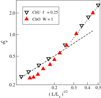
Figure 1: The length dependence of the mean conductance $\langle g\rangle$ for quasi-one dimensional chiral systems of length $L_{z}$ and fixed width $L=65\,a$. The energy is $E=0$. Due to the chiral symmetry of the model, the crossover from the Ohmic $1/L_{z}$-behavior (dotted line) to the $1/\sqrt{L_{z}}$ dependence (dashed line) is observed, in agreement with theoretical predictions [22]. Two models with chiral unitary (ChU: $f=0.25\,h/e$) and chiral orthogonal (ChO: $W/t_{0}=1$) symmetry, defined in section 2, were considered.

In this paper we review some results of our recent investigations on electric transport properties of two dimensional chiral systems. In the following section we briefly introduce the models studied. In section 4, we summarize our findings for the Lyapunov exponents, the critical conductance and its probability distribution, and show recent calculations for the density of states. Of special interest is the scaling analysis of the diverging critical electronic states at $E=0$ [24, 30, 31].

2 Models

In the absence of diagonal disorder the single-band tight-binding Hamiltonian defined on the sites $n$ of a two-dimensional bricklayer or square lattice with lattice constant $a$ reads

$${\cal H}=\sum_{\langle n\neq n^{\prime}\rangle}t_{nn^{\prime}}c_{n}^{\dagger}c_{n^{\prime}},$$ (3)

where the sum is over nearest neighbors only. The random disorder is incorporated in the hopping terms, which also determine the symmetry of the problem. Square lattice and bricklayer lattice differ only in the absence of every other vertical bond in the latter and so the coordination number is reduced to three (see Fig. 2).

2.1 Unitary symmetry

To describe a disordered chiral 2D system with broken time-reversal symmetry, the hopping terms in the (transversal) $x$ direction are chosen to acquire complex phases and are defined as

$$t_{x}=t_{0}e^{i\theta_{x,z;x\pm a,z}},$$ (4)

where for a bricklayer lattice the phases $\theta_{x,z;x+a,z}=\theta_{x,z+2a;x+a,z+2a}-\frac{2\pi e}{h}\Phi_{x,z}$ are determined by the total flux threading the plaquette at $(x,z)$

$$\Phi_{x,z}=\frac{p}{q}\frac{h}{e}+\phi_{x,z}.$$ (5)

Here, $p$ and $q$ are mutual prime integers and the magnetic flux density perpendicular to the two-dimensional lattice $B=ph/(qe2a^{2})$ is described by the number $p/q$ of magnetic flux quanta $h/e$ per plaquette $2a^{2}$. This differs from the random flux model studied previously [32], where the constant magnetic field part was absent. The random part is generated by the local fluxes $\phi_{x,z}$, which are uniformly distributed $-f/2\leq\phi_{x,z}\leq f/2$ with zero mean. The disorder strength $f$ can be varied within the interval from $f/(h/e)=0$ to $f/(h/e)=1$.

2.2 Orthogonal symmetry

For the chiral orthogonal symmetry, we consider two different models. Both are defined on a square lattice. In the first, we set $t_{z}/t_{0}=1$ and take the disordered hopping terms as random real numbers that are defined as

$$t_{x}=t_{0}\exp\frac{W}{t_{0}}\varepsilon,$$ (6)

where {$\varepsilon$} is a set of uncorrelated random numbers with box probability distribution $|\varepsilon|\leq 1/2$. The strength of the disorder was varied in the range $W/t_{0}=2$ to $W/t_{0}=10$. In the second model, the transfer terms in both the $x$ and $z$ direction are random numbers which are box-distributed about $t_{0}$ within the interval [$t_{0}-W_{s}/2$, $t_{0}+W_{s}/2$] with possible disorder strengths $0\leq W_{s}/t_{0}\leq 2$. In the latter model, single sites may get isolated and decoupled from the remaining 2D lattice for $W/t_{0}\to 2$.

2.3 Symplectic symmetry

The off-diagonal disorder as given by Eq. (6) with $W/t_{0}=4$ was used in the chiral symplectic model, where we consider a chiral version of the Ando model [5, 33]. The hopping terms $t_{nn^{\prime}}$ are now $2\times 2$ matrices

$$t_{\parallel}=t_{0}\left(\begin{array}[]{ll}c&-s\\ -s&c\end{array}\right),\quad t_{\perp}=t_{x}\left(\begin{array}[]{ll}c&is\\ -is&c\end{array}\right),$$ (7)

where $c^{2}+s^{2}=1$, $s=1/2$, and the disorder in the hopping $t_{x}$ is given by Eq. (6).

2.4 Lattice topology

The two-dimensional lattices of size $L\times L_{z}$ on which the above models are defined, are either a regular square lattice or a bricklayer lattice which mimics the honeycomb lattice (Fig. 2). The width $L$ and the length $L_{z}$ of the lattice are taken to be similar $L_{z}\simeq L$ for the investigations of the DOS and for the conductance, whereas quasi-one-dimensional samples with $L_{z}\sim 10^{9}$ lattice units are used in the analysis of the scaling properties of the models.

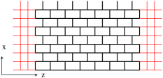
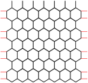
Figure 2: The bricklayer lattice (left) shares the topology of the honeycomb lattice (right). The red lines display the attached perfect semi-infinite leads used in the calculation of the scaling variables $z_{i}$ and the two-terminal conductance.

3 Numerical methods

For the numerical calculation of the two-terminal conductance, we attach two ideal (without disorder) semi-infinite leads to the finite sample having width $L$ and length $L_{z}$ and apply the well known Economou-Soukoulis formula [34]

$$g=\frac{e^{2}}{h}\,\textrm{Tr}~{}T^{\dagger}T=\frac{e^{2}}{h}\sum_{i=1}^{N_{\rm open}}\frac{1}{\cosh^{2}(x_{i}/2)},$$ (8)

where $T$ is the corresponding transmission matrix and the $x_{i}$ parameterize the eigenvalues of the hermitian matrix $T^{\dagger}T$. The parameter $N_{\rm open}$ determines the number of open channels in the attached leads. Owing to the disorder, the conductance is a statistical variable. Therefore, an ensemble of finite samples, which differ only in the microscopic realization of the disorder, is considered and the mean value, the variance, and probability distribution of the conductance is evaluated using the algorithm described in [35].

We define the dimensionless quantities $z_{i}=x_{i}L/L_{z}$ to be used for the scaling analysis in the vicinity of the critical point [36]. In the limit $L_{z}\gg L$, the ratio $z_{1}/(2L)$ converges to the smallest Lyapunov exponent $\gamma=\lim_{L_{z}\to\infty}x_{1}/(2L_{z})$ where $x_{1}$ is the smallest positive eigenvalue of $\ln(T^{\dagger}T)$. We calculated numerically the first two parameters $z_{1}$ and $z_{2}$ for Q1D systems of length up to $L_{z}\sim 10^{8}L$ in order to achieve a relative uncertainty for $z_{1}$ of order of $10^{-4}$. The data obtained for $z_{1}(E,L)$ and $z_{2}(E,L)$ were fitted to scaling formulae (1) and (2).

4 Properties of chiral systems

In this section, we summarize our numerical results obtained for various disordered systems obeying chiral symmetry.

4.1 Scaling variables $z_{i}$

The calculated spectrum of scaling variables $z_{i}=x_{i}L/L_{z}$ is strongly influenced by the presence of the chiral symmetry [20, 22]. They take on also negative values for chiral unitary systems. Our data [29] confirmed that

$$|z_{2a-1}|=|z_{2a}|=c\left[a-1/2\right]$$ (9)

for an even number of open channels, and

$$|z_{i}|=\left\{\begin{array}[]{ll}c\ {\rm Int}[a/2]&{\rm Dirichlet~{}BC}\\ (c/2)\ [a-1/2]&{\rm periodic~{}BC}\end{array}\right.$$ (10)

for an odd number of channels. From Eq. (10) it follows that the mean value of the smallest $z_{1}$ is zero.

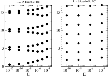
Figure 3: The spectrum of scaling variables $|z_{i}|$ for the Q1D systems with chiral orthogonal symmetry. A lattice $L\times L_{z}$ with square topology is considered with an odd value $L=65\,a$ and two boundary conditions (BC) Dirichlet (left) and periodic (right) imposed in the transversal direction. For Dirichlet BC, the model is chiral orthogonal at the band center $E=0$ and $z_{1}(E=0)=0$, in agreement with Eq. (10). The symmetry changes to orthogonal for non-zero energy $E$. Note the degeneracy in the spectrum of scaling variables for the Dirichlet BC. This degeneracy is broken for non-zero energies $E$. There is no chiral symmetry for periodic BC. The disorder strength in the vertical hopping (4) is $W=5$. Similar results for the chiral unitary symmetry were published in [29].

The same relations hold also for chiral orthogonal systems. Figure 3 shows the spectrum of scaling variables for $N_{\rm open}$ odd and two types of boundary conditions. The numerical data indeed confirm that $z_{1}=0$ when Dirichlet BC are imposed. This is a reason for the non-Ohmic behavior of the mean conductance shown in Fig. 1. Also, Fig. 3 shows that the degeneracy of the spectrum of absolute values $|z_{i}|$ is lifted for any non-zero energy. A more detailed analysis of the scaling variables $z_{i}$ for the chiral unitary system is given in Ref. [29].

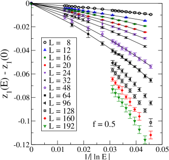
Figure 4: The smallest scaling variable $z_{1}$ for chiral unitary systems without a constant magnetic field, calculated on the bricklayer lattice. The number of open channels $N_{\rm open}$ is identical with the width of the layer. Periodic BC were used in the transversal direction. Note that the energy decreases up to $E/t_{0}\sim 10^{-30}$. Since quartic precision in the numerical calculations is necessary to treat such energies, we were able to calculate the scaling variables $z_{i}$ for these energies only for narrow samples ($L\leq 24$), due to the accuracy and CPU requirements.

4.2 Scaling analysis

Scaling theory predicts that in the vicinity of the critical point $E=0$, the smallest scaling variable $z_{1}$ is a function of only one parameter,

$$z_{1}(E,L)=F(\chi)$$ (11)

where $\chi=\ln L/\ln(\xi(E)/\xi_{0})$, and $\xi(E)$ is the correlation length

$$\ln\frac{\xi(E)}{\xi_{0}}\sim\left|\,\ln\left(\frac{E_{0}}{|E|}\right)\,\right|^{\kappa}$$ (12)

with unknown energy parameter $E_{0}$ and exponent $\kappa$.

Figure 4 shows typical numerical data obtained in the vicinity of the chiral critical point. The data confirm that both $z_{1}$ and $z_{2}$ can be described as a function of $\ln E$. However, a logarithmic energy dependence of $\xi(E)$, given by Eq. (12) can be observed only for very small values of the energy, typically $|E/t_{0}|<10^{-8}$.

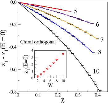
Figure 5: Scaling of the smallest scaling variable $z_{1}$ for chiral orthogonal models with hopping terms $t_{x}$ given by Eq. (6). The disorder strength $W/t_{0}$ is given in the Figure. The scaling variable $\chi$ on the horizontal axis is given by Eqs. (1) and (2) with $\xi_{0}=1$, $E_{0}\approx-4.5\,t_{0}$ and the exponent $\kappa$ close to the value 2/3 [37]. The inset shows the disorder dependence of $z_{1}(E=0)$ for $L=96\,a$.

For orthogonal and symplectic models as described in section 2 with disorder given by (6), we verified the scaling behavior (12) for each given disorder strength. In all systems we used periodic BC and even $N_{\rm open}$. This choice enables us also to compare systems with and without a constant magnetic field. Systems with odd $N_{\rm open}$ and Dirichlet BC are numerically not accessible since the smallest $z_{i}$ is zero for $E=0$ and very small for non-zero energy (Fig. 3).

We fit the numerical data for $z_{1}$ and $z_{2}$ to the polynomial function of $\chi$ and extract the critical exponent $\kappa$. We found that for all models $\kappa\approx 2/3$, in agreement with previous theoretical predictions [31, 24, 30]. As an example, we show in Fig. 5 the result of our scaling analysis for the chiral orthogonal model and various strengths of the disorder. The disorder dependence of $z_{1}(E=0,W)$ is plotted in the inset. This shows that the the value of the disorder $W$ represents an extra parameter that defines the respective model.

Although the addition of a constant magnetic field to the chiral orthogonal model breaks the time-reversal symmetry, it does not influence the value of the exponent $\kappa\approx 2/3$. The only exception is the chiral unitary model without constant magnetic field where $\kappa\simeq 1/2$ [32] (the raw data for this model are shown in Fig. 4). More details about the scaling at chiral quantum critical points can be found elsewhere [37].

We did not succeed in obtaining the logarithmic scaling from the raw data for the mean conductance [29, 26]. The reason is that for each particular sample the conductance is given as a sum of contributions of all channels. Since the sum $z_{1}+z_{2}$ is almost constant also for non-zero energies, the conductance depends only very weakly on the energy in the vicinity of the critical point. This tiny energy dependence, if any at all, cannot be extracted from our numerical data.

4.3 Conductance

At the critical point, the probability distribution of the conductance $P(g)$ does not depend on the size of the system, and possesses the typical shape for a given universality class. In Fig. 6 we show the conductance distribution for the chiral unitary system without a constant magnetic field. The data confirm that the distribution does not depend on the strength of the disorder $f$, which in this case measures the fluctuation of the flux through the plaquettes. Since the disorder is weak, the mean value of the conductance is large, and decreases when the disorder increases, as shown in the inset. The critical distribution is Gaussian with a universal width, var $g=0.187$.

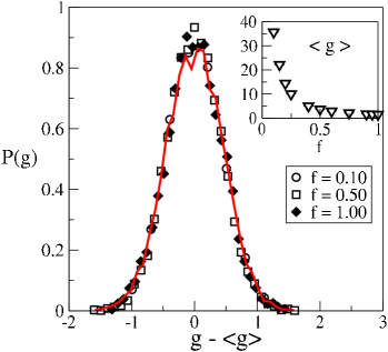
Figure 6: The probability distribution $P(g-\langle g\rangle)$ for the chiral unitary system without magnetic field and three different values of $f$. The width of the distribution var $g\approx 0.187$ does not depend on $f$. The solid line is the conductance distribution for the chiral unitary model with $f=0.5\,h/e$ and with an additional magnetic field $B=(1/12)\,h/(ea^{2})$ ($L/a=72$, mean conductance $\langle g\rangle=2.82$, var $g=0.207$). The inset shows the mean conductance $\langle g\rangle_{c}$ for various values of the random field $f$. Square samples of size $257\times 257$ were considered with Dirichlet BC in the transversal direction. Note that the strength of the disorder is limited in the present model. Even for $f=1\,h/e$, we get a rather large mean conductance, $\langle g\rangle=1.45\,e^{2}/h$.

Of particular interest is the comparison of the two unitary chiral systems that differ from each other only by the presence of a constant magnetic field. As discussed in the previous section, these two systems exhibit a different critical exponent $\kappa$. Surprisingly, the conductance distributions for these two models are almost identical as shown in Fig. 6. Also, the mean conductance is larger than 1 even in the case of strongest disorder possible ($f=1\,h/e$). Therefore, our chiral unitary model does not allow studies of strongly disordered chiral systems.

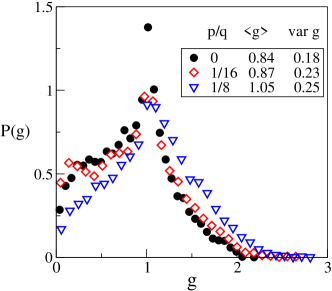
Figure 7: The conductance distribution for the two-dimensional disordered chiral orthogonal model on a square lattice with random hopping terms (6), and with a constant magnetic field, $B=(p/q)\,h/ea^{2}$. The disorder strength is $W/t_{0}=5$, and the size of the system $L/a=64$. The legend gives the ratio $p/q$ which determines the magnetic field and corresponding mean conductance and the variance. Note the typical non-analytical form of the distribution at $g=1\,e^{2}/h$ [38].

Smaller values of the critical conductance can be obtained for systems with random hopping terms as given by Eq. (6). Figure 7 shows the critical conductance distribution for system with real hopping terms given by Eq. (6) with disorder $W=5$ and various strengths of the constant magnetic field. While the system without magnetic field belongs to the chiral orthogonal universality class, the constant magnetic field changes the symmetry to chiral unitary. In spite of the different symmetry classes, no significant difference between the critical distributions is observed. Also the critical exponent $\kappa\approx 2/3$ is the same for both models [37].

4.4 Density of states

In many ‘standard’ disordered models, the density of states can be considered to be constant in the critical region. A very strong energy dependence of the DOS can affect the accuracy of the numerical scaling. A typical example is the metal-insulator transition in the band tails (see, for instance, [39]). Recently it was found that chiral unitary models can exhibit a very narrow dip in the DOS at the band center [27]. It has been suggested [21, 40] that these ‘microgaps’ appearing in disordered chiral models are the consequence of the non-perturbative ergodic regime. This can happen for times large compared with the diffusion time when the localization length exceeds the sample size.

As an example, the DOS in the vicinity to the chiral unitary critical point is shown in Fig. 8. The energy range of the DOS depression gets narrower with increasing RMF disorder strength for zero constant magnetic field but it becomes broader in the case of a finite constant magnetic field [27]. In the latter case, two additional quantum Hall critical points (QHCPs) showing the usual power-law divergence with critical exponent $\nu\simeq 2.4$ [26] exist symmetrically about the chiral point at $E=0$. Within the achieved uncertainty this value for the chiral quantum Hall case obtained for a bricklayer lattice is compatible with the recent high-precision estimates $\nu\simeq 2.6$ [41, 42] obtained for the Chalker-Coddington network model [43]. With increasing disorder, the QHCPs move further apart [26] and so they can be easily distinguished from the chiral one remaining at $E=0$ and studied here.

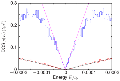
Figure 8: The depression in the density of states $\rho(E)$ near the quantum critical point at $E=0$ for the random magnetic flux model with (upper blue curve) and without (lower red curve) a spatial constant magnetic flux density defined on a bricklayer lattice. The histogram bin-width is about $4\times 10^{-6}$. The dip in the DOS depends on both the disorder strength and the sample size. The brown and magenta solid lines are fitting curves [27]. The RMF strength and system size are $f=0.5\,h/e$, $L=L_{x}=96\,a$ for $B=0$, and $f=0.5\,h/e$, $L=L_{x}=120\,a$ in the case of $B=(1/12)\,h/(2ea^{2})$, respectively.

To check whether this is a general feature of systems with chiral symmetry, we calculated numerically also the density of states for chiral orthogonal and for chiral symplectic models. The results are shown in Figs. 9 and 10. Similar to the case of chiral unitary symmetry, the chiral symplectic system shows a spectral gap in the DOS at $E=0$. For a square system $L=64$ and $W=3$ hopping disorder in both spatial directions, the narrow gap is still visible. With increasing disorder strength or system size, however, the gap becomes narrower until it seems to disappear due to the insufficient numerical resolution.

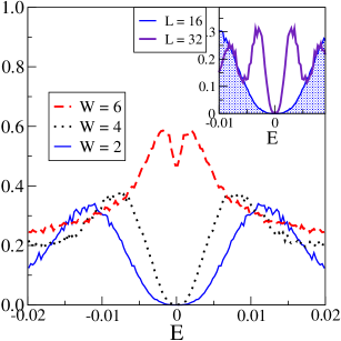
Figure 9: The density of states for the chiral symplectic model calculated by diagonalizing $2\times 10^{5}$ samples of size $16\times 16$. A dip in the density of states is present only for weak disorder and small size of the lattice, but disappears when disorder and/or lattice size increases. The inset shows the density of states for disorder $W=2$ and $L=16$ and $L=32$.

In the chiral orthogonal case, instead of a dip, an extra peak is seen on top of the disorder broadened DOS at the quantum critical point $E=0$. This result was obtained for a square lattice model with random hopping in both directions where van Hove singularities appear at the band center and not at $E/t_{0}=\pm 1$ as for the bricklayer (hexagonal) lattice. An explanation for the occurrence of the extra peak is the possible isolation of single lattice sites that become disconnected from the remaining system with increasing disorder. These sites contribute to the DOS with eigenvalues close to zero.

5 Conclusion

Two dimensional systems with chiral symmetry exhibit interesting new physical properties, not observed in standard disordered models. The most striking feature is that the existence of a chiral quantum critical point is determined by the boundary conditions and by the parity of the size of the system. The chiral critical point coincides with narrow structures in the energy dependence of the density of states which depend both on the disorder strength and on the system size. To study the intriguing scaling behavior, a logarithmic scaling ansatz is necessary which replaces the usual power-law dependence applied in ordinary Anderson localization with diagonal disorder.

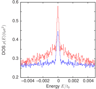
Figure 10: The density of states for the chiral orthogonal model defined on a square lattice with real random hopping in both directions obtained by diagonalization of more than $2\times 10^{4}$ samples of size $80\times 80$ and disorder strengths $W_{s}/t_{0}=1.0$ (blue) and $W_{s}/t_{0}=1.5$ (red). No dip but an extra peak is observed in the density of states close to the quantum critical point $E=0$.

Owing to the logarithmic energy dependence of the correlation length, the critical region is very narrow. Typically, it is narrower than the $10^{-8}$th part of the bandwidth. This makes the scaling analysis of the chiral critical behavior rather difficult. To achieve relevant data with sufficient accuracy, extremely long systems must be calculated, in some cases with quartic precision (up to 34 digits) of arithmetic operations. This is probably the reason why the logarithmic scaling was not observed in previous numerical studies [29, 44, 45, 46, 47]. Our numerical data indicate that all chiral systems can be divided into two classes: the first one consists of only one model with random magnetic flux and zero magnetic field. For this model, we observed that the critical exponent which governs logarithmic energy dependence of the correlation length is $\kappa\simeq 1/2$. For all other models, the critical exponent is $\kappa\simeq 2/3$, independent of the symmetry.

PM thanks Project VEGA 0633/09 for financial support.

References

- Abrahams et al. [1979] E. Abrahams, P. W. Anderson, D. C. Licciardello, and T. V. Ramakrishnan, Phys. Rev. Lett. 42, 673 (1979).
- Soukoulis and Economou [1984] C. M. Soukoulis and E. N. Economou, Phys. Rev. Lett. 52, 565 (1984).
- Hikami et al. [1980] S. Hikami, A. I. Larkin, and Y. Nagaoka, Prog. Theor. Phys. 63, 707 (1980).
- Evangelou and Ziman [1987] S. N. Evangelou and T. Ziman, J. Phys. C: Solid State Phys. 20, L235 (1987).
- Ando [1989] T. Ando, Phys. Rev. B 40, 5325 (1989).
- Asada et al. [2002] Y. Asada, K. Slevin, and T. Ohtsuki, Phys. Rev. Lett. 89, 256601 (2002).
- Asada et al. [2004] Y. Asada, K. Slevin, and T. Ohtsuki, Phys. Rev. B 70, 035115 (2004).
- Schweitzer [1995] L. Schweitzer, J. Phys.: Condens. Matter 7, L281 (1995).
- Asada et al. [2003] Y. Asada, K. Slevin, and T. Ohtsuki, J. Phys. Soc. Jap. 72, 145 (2003).
- Schweitzer et al. [1984] L. Schweitzer, B. Kramer, and A. MacKinnon, J. Phys. C 17, 4111 (1984).
- Huckestein et al. [1992] B. Huckestein, B. Kramer, and L. Schweitzer, Surface Science 263, 125 (1992).
- Huckestein and Schweitzer [1994] B. Huckestein and L. Schweitzer, Phys. Rev. Lett. 72, 713 (1994).
- Wang et al. [1998] X. Wang, Q. Li, and C. M. Soukoulis, Phys. Rev. B 58, 3576 (1998).
- Schweitzer and Markoš [2005] L. Schweitzer and P. Markoš, Phys. Rev. Lett. 95, 256805 (2005).
- Inui et al. [1994] M. Inui, S. A. Trugman, and E. Abrahams, Phys. Rev. B 49, 3190 (1994).
- Evangelou and Katsanos [2003] S. N. Evangelou and D. E. Katsanos, J. Phys. A: Math. Gen. 36, 3237 (2003).
- Gade and Wegner [1991] R. Gade and F. Wegner, Nucl. Phys. B360, 213 (1991).
- Gade [1993] R. Gade, Nucl. Phys. B398, 499 (1993).
- Miller and Wang [1996] J. Miller and J. Wang, Phys. Rev. Lett. 76, 1461 (1996).
- Brouwer et al. [1998] P. W. Brouwer, C. Mudry, B. D. Simons, and A. Altland, Phys. Rev. Lett. 81, 862 (1998).
- Altland and Simons [1999] A. Altland and B. D. Simons, J. Phys. A: Math. Gen. 32, L353 (1999).
- Mudry et al. [1999] C. Mudry, P. W. Brouwer, and A. Furusaki, Phys. Rev. B 59, 13221 (1999).
- Fabrizio and Castelliani [2000] M. Fabrizio and C. Castelliani, Nucl. Phys. B 583, 542 (2000).
- Motrunich et al. [2002] O. Motrunich, K. Damle, and D. A. Huse, Phys. Rev. B 65, 064206 (2002).
- Evers and Mirlin [2008] F. Evers and A. D. Mirlin, Rev. Mod. Phys. 80, 1355 (2008).
- Schweitzer and Markoš [2008] L. Schweitzer and P. Markoš, Phys. Rev. B 78, 205419 (2008).
- Schweitzer [2009] L. Schweitzer, Phys. Rev. B 80, 245430 (2009).
- Sittler and Hinrichsen [2002] L. Sittler and H. Hinrichsen, J. Phys. A: Math. Gen. 35, 105351 (2002).
- Markoš and Schweitzer [2007] P. Markoš and L. Schweitzer, Phys. Rev. B 76, 115318 (2007).
- Mudry et al. [2003] C. Mudry, S. Ryu, and A. Furusaki, Phys. Rev. B 67, 064202 (2003).
- Hatsugai et al. [1997] Y. Hatsugai, X.-G. Wen, and M. Kohmoto, Phys. Rev. B 56, 1061 (1997).
- Markoš and Schweitzer [2010] P. Markoš and L. Schweitzer, Phys. Rev. B 81, 205432 (2010).
- Markoš and Schweitzer [2006] P. Markoš and L. Schweitzer, J. Phys. A 39, 3221 (2006).
- Economou and Soukoulis [1981] E. N. Economou and C. M. Soukoulis, Phys. Rev. Lett. 46, 618 (1981).
- Pendry et al. [1992] J. B. Pendry, A. MacKinnon, and P. J. Roberts, Proc. R. Soc. London A 437, 67 (1992).
- Kramer and MacKinnon [1993] B. Kramer and A. MacKinnon, Rep. Prog. Phys. 56, 1469 (1993).
- Schweitzer and Markoš [2011] L. Schweitzer and P. Markoš, to be published (2011).
- Markoš [2006] P. Markoš, acta physica slovaca 56, 561 (2006).
- Brndiar and Markoš [2006] J. Brndiar and P. Markoš, Phys. Rev. B 74, 153103 (2006).
- Simons and Altland [2001] B. D. Simons and A. Altland, in Theoretical Physics at the End of the XXth Century, edited by Y. Saint-Aubin and L. Vinet (Springer, 2001), CRM Series in Mathematical Physics, pp. 451–558.
- Slevin and Ohtsuki [2009] K. Slevin and T. Ohtsuki, Phys. Rev. B 80, 041304 (2009).
- Amado et al. [2011] M. Amado, A. V. Malyshev, A. Sedrakyan, and F. Domínguez-Adame, Phys. Rev. Lett. 107, 066402 (2011).
- Chalker and Coddington [1988] J. T. Chalker and P. D. Coddington, J. Phys. C: Solid State Phys. 21, 2665 (1988).
- Cerovski [2000] V. Z. Cerovski, Phys. Rev. B 62, 12775 (2000).
- Cerovski [2001] V. Z. Cerovski, Phys. Rev. B 64, 161101(R) (2001).
- Eilmes et al. [2001] A. Eilmes, R. A. Römer, and M. Schreiber, Physica B 296, 46 (2001).
- Eilmes and Römer [2004] A. Eilmes and R. A. Römer, phys. stat. sol. (b) 241, 2079 (2004).