Non-Gaussian bubbles in the sky

Abstract

We point out a possible generation mechanism of non-Gaussian bubbles in the sky due to bubble nucleation in the early universe. We consider a curvaton scenario for inflation and assume that the curvaton field $\phi$, whose energy density is subdominant during inflation but which is responsible for the curvature perturbation of the universe, is coupled to another field $\sigma$ which undergoes false vacuum decay through quantum tunneling. For this model, we compute the skewness of the curvaton fluctuations due to its interaction with $\sigma$ during tunneling, that is, on the background of an instanton solution that describes false vacuum decay. We find that the resulting skewness of the curvaton can become large in the spacetime region inside the bubble. We then compute the corresponding skewness in the statistical distribution of the cosmic microwave background (CMB) temperature fluctuations. We find a non-vanishing skewness in a bubble-shaped region in the sky. It can be large enough to be detected in the near future, and if detected it will bring us invaluable information about the physics in the early universe.

I Introduction

Inflation, a stage of accelerated expansion in the very early universe, is now widely accepted as part of the standard evolutionary scenario of the universe. On the other hand, many models of inflation have been proposed but we are still far from being able to narrow down the possible models sufficiently. Among those many models of inflation, much attention has been paid recently to the ones based on string theory Kachru:2003aw , which is considered to be a promising candidate for the ultimate unified theory. In particular, it is of great interest if the string theory landscape Susskind:2003kw , in which there are many local minima, or false vacua, and the universe jumps from one minimum to another by quantum tunneling, can be observationally tested Yamauchi:2011qq ; Yamamoto:1996qq . Quantum tunneling of a scalar field with gravity is usually treated with the Coleman-De Luccia (CDL) instanton method Coleman:1980aw , where the evolution of a scalar field is described with an O(4)-symmetric instanton, which is a solution of the Euclidean equations of motion. Motivated by the string landscape, inflation models with multi-scalar fields and/or with tunneling are now keenly studied. Extension of the CDL instanton method to a multi-scalar field system is already discussed in Sugimura:2011tk . In those studies, however, many inflation models have been proposed, and now it is important to distinguish those models by observation.

Observations of the power spectrum of CMB temperature anisotropies have convinced us of the existence of an inflationary stage in the very early universe. On top of that, if a non-Gaussian feature such as skewness or bispectrum is detected in the CMB anisotropy, it will have a strong impact on the physics of the early universe Komatsu:2010fb . In particular, since any single-field slow-roll inflation model with canonical kinetic term predicts almost Gaussian fluctuations Maldacena:2002vr , any non-zero non-Gaussianity will exclude all these models. Observations of non-Gaussianity use templates, such as local type Komatsu:2001rj , equilateral type Creminelli:2005hu , and orthogonal type Senatore:2009gt , in order to increase the statistical significance. However, since all of these templates assume statistical isotropy, there may be anisotropic non-Gaussianities which may not have been detected by these templates.

In this letter, we study a multi-field model in which a nonlinear interaction between two scalar fields, one of which being responsible for the curvature perturbation of the universe (that is, for the formation of the large scale structure) and the other for quantum tunneling via a CDL instanton, induces an anisotropic non-Gaussianity. To be specific, we introduce an inflaton field $\Phi$ that realizes slow-roll inflation, a tunneling field $\sigma$ that governs the tunneling dynamics, and a curvaton field $\phi$ that contributes to the curvature perturbation of the universe Lyth:2002my ; Sasaki:2006kq .

The inflaton dominates the energy density of the universe during inflation but rapidly decays to radiation after the end of inflation, On the other hand, the energy density of the curvaton field is negligible during inflation but its decay is delayed after inflation so that it gradually begins to dominate the universe.

Approximating the universe during inflation by an exact de Sitter spacetime, the inflaton behaves as a cosmic clock and determines an appropriate time-slicing, namely, a spatially flat time-slicing of the de Sitter spacetime. In this setup, assuming that the energy scale associated with the tunneling field is much smaller than the energy scale of inflation, the bubble nucleation can be well described by a single-field CDL instanton with no backreaction to the geometry, that is, on the exact de Sitter background Coleman:1980aw ; Yamamoto:1996qq .

The curvaton $\phi$ is affected by the background bubble through a coupling with the tunneling field $\sigma$. For simplicity and definiteness, we consider a potential of the form, $V_{\mathrm{int}}(\sigma,\phi)=\tilde{\lambda}(\sigma)\phi^{3}$ . Assuming that $V_{\mathrm{int}}(\sigma,\phi)$ is non-vanishing only at or inside the bubble wall, we expect that $\phi$ may have a spatially localized, bubble-shaped non-Gaussianity due to the background bubble-shaped configuration of $\sigma$. This leads to an anisotropic, bubble-shaped skewness of the CMB temperature anisotropy.

This paper is organized as follows. We first illustrate the background spacetime and the configuration of the bubble. Next, we briefly review a useful formalism for computing the equal-time $N$-point functions, the tunneling in-in formalism, and calculate the skewness of the curvaton fluctuations. Then we demonstrate that a sky map of an anisotropic non-Gaussian parameter $f_{\rm NL}$ in our model. Finally, we end with a few concluding remarks.

II Background Evolution

Let us start from a brief description of de Sitter spacetime birrell-davies ; Yamamoto:1996qq . A Lorentzian 4-dimensional de Sitter spacetime is O(4,1)-symmetric, which is obtained by analytical continuation of an O(5)-symmetric 4-dimensional Euclidean sphere, as illustrated in Fig. 1.

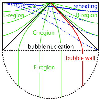
Figure 1: Penrose-like diagram of bubble nucleating universe, where a half of Euclidean region (bottom) and Lorentzian region after bubble nucleation (top) are shown The blue dot-dashed lines are surfaces of constant cosmic time, the green solid lines those of uniform tunneling field, and the red solid line the location of the bubble wall.

Among various coordinatization of the spacetime, the uniform tunneling field slicing is most appropriate to see O(4)(O(3,1))-symmetry of the CDL instanton, which corresponds to the time-slicing inside the bubble that describes a spatially homogeneous and isotropic open universe. For brevity, let us call it open slicing. Open slicing in the C-region in Fig. 1 is a time-like slicing, an the metric in the C-region may be expressed as

$$ds^{2} =\frac{1}{H^{2}}\Bigl{(}d\chi^{2}+\sin^{2}\chi\left(-d\tau^{2}+\cosh^{2}\tau\,d\Omega_{2}^{2}\right)\Bigr{)}\,,$$ (1)

where $-\infty<\tau<\infty$ and $0\leq\chi\leq\pi$, and $d\Omega_{2}^{2}$ is the metric on the unit 2-sphere. Theses coordinates can be extended to the other regions of the spacetime by analytical continuation:

$$\tau=r_{\mathrm{R}}+i\pi/2=r_{\mathrm{L}}-i\pi/2=ir_{\mathrm{E}}\,,$$ (2)

$$\chi=it_{\mathrm{R}}=-it_{\mathrm{L}}=t_{\mathrm{E}}\,,$$ (3)

where $(t_{\mathrm{R}},r_{\mathrm{R}})$, $(t_{\mathrm{L}},r_{\mathrm{L}})$ and $(t_{\mathrm{E}},r_{\mathrm{E}})$ are the coordinates for the R-, L-, and E-regions, respectively, in Fig. 1.

The metric for the flat time-slicing is

$$ds^{2}=-dt^{2}+a^{2}(t)\left(dr^{2}+r^{2}d\Omega_{2}^{2}\right)\,;\ \,a(t)=H^{-1}e^{Ht}\,.$$ (4)

As mentioned in the introduction, the $t=const.$ slices are on which the inflaton is uniform, and give the cosmic rest frame of our universe.

Let us briefly describe the bubble configuration of $\sigma$ under the thin-wall approximation. The O(4)-symmetric CDL instanton for $\sigma$ can be described as a function of $\chi$, which we denote by $\bar{\sigma}(\chi)$ hereafter. We denote the wall radius by $R_{\rm W}$. Hence

$$\bar{\sigma}(\chi)=\left\{\begin{array}[]{ll}\sigma_{\rm T}\quad\mbox{for}{}&0\leq\chi<HR_{\rm W}\,,\\ \sigma_{\rm F}\quad\mbox{for}{}&HR_{\rm W}<\chi\leq\pi\,.\end{array}\right.$$ (7)

Though $\bar{\sigma}$ is homogeneous in the R- or L-regions, the physical bubble radius $\ell_{\rm W}(t)$ on flat slices increases as time goes on. We take the origin $r=t=0$ of the flat slicing metric (4) to be the center of the bubble at the time of nucleation. Then the relations between the coordinates in the metrics (1) and (4) are $\cos\chi=\cosh Ht-(1/2)e^{Ht}r^{2}$ and $\sin\chi\cosh\tau=e^{Ht}r$, which gives $\ell_{\rm W}(t)=a(t)\sqrt{1+e^{-2Ht}-2e^{-Ht}\cos HR_{\rm W}}$. As seen from this expression, a bubble once nucleated with radius $\ell_{\rm W}(0)$ ($\approx R_{\rm W}$ for $HR_{\rm W}\ll 1$) expands to the Hubble horizon scale within one or two $e$-folds of time, $\Delta t\sim H^{-1}$, and then expands comovingly as $\ell_{\rm W}(t)\sim a(t)$.

It should be noted that models with multiple nucleation is possible. If those bubbles do not interact each other, we can take into account the effect of all bubbles by summing up the effect of each bubble. Hereafter, we consider a model with a single bubble for simplicity.

III Non-Gaussianity Generation

III.1 Effective Action on Instanton Background

Here we calculate the skewness in the curvaton fluctuations on the single bubble background. We consider the Lagrangian for the curvaton $\phi$ as

$$\mathcal{L}_{\phi}=-\sqrt{-g}\left(\frac{1}{2}g^{\mu\nu}\partial_{\mu}\phi\partial_{\nu}\phi+\frac{m^{2}}{2}\phi^{2}+V_{\mathrm{int}}(\sigma,\phi)\right)\,,$$ (8)

where $m^{2}\ll H^{2}$. We expand the above by setting $\phi=\phi_{0}+\delta\phi$, where $\phi_{0}$ is a homogeneous classical part and $\delta\phi$ is a quantum fluctuation. We assume that $\phi_{0}$ is approximately constant during inflation, and we concentrate on the evolution of $\delta\phi$. Further, for simplicity, we assume $V_{\mathrm{int}}(\sigma,\phi)$ is non-vanishing only on the wall. Hence we approximate it as $V_{\mathrm{int}}(\sigma,\phi)=\lambda\,\phi^{3}H\,\delta(\chi-HR_{\rm W})$ with $\lambda H=\int^{\pi}_{0}\mathrm{d}\chi\tilde{\lambda}(\bar{\sigma}(\chi))$ . Then the Lagrangian for $\delta\phi$ is given as $\mathcal{L}_{\delta\phi}=\mathcal{L}_{0}+\mathcal{L}_{I}$, where $\mathcal{L}_{0}$ is free-part and $\mathcal{L}_{I}$ is interaction-part,

$$\mathcal{L}_{0} =-\sqrt{-g}\left(\frac{1}{2}g^{\mu\nu}\partial_{\mu}\delta\phi\,\partial_{\nu}\delta\phi\,+\frac{1}{2}\left(m^{2}+\delta m^{2}\right)\delta\phi^{2}\right),$$

$$\mathcal{L}_{I} =-\sqrt{-g}\,\lambda H\delta\left(\chi-HR_{\rm W}\right)\delta\phi^{3}\,,$$ (9)

where $\delta m^{2}\equiv 6\lambda H\phi_{0}\delta(\chi-HR_{\rm W})$.

III.2 Quantum Field Theory on the Instanton Background

To calculate the quantum fluctuations on the instanton background, we extend the in-in formalism to Euclidean spacetime, which we call the tunneling in-in formalism. This formalism is based on the WKB analysis of a tunneling wave function for free theory Tanaka:1993ez ; Yamamoto:1993mp to the case with nonlinear interactions. A detailed derivation will be given elsewhere preparation .

The tunneling in-in formalism tells us that the $N$-point function of $\delta\phi$ is given by

$$\Big{<}\delta\phi(x_{1})\delta\phi(x_{2})\cdots\delta\phi(x_{N})\Big{>}$$

$$= \frac{\left<{0}\left|{P\,\delta\phi(x_{1})\delta\phi(x_{2})\cdots\delta\phi(x_{N})e^{i\int_{C\times\Sigma_{t}}dtd^{3}x\,\mathcal{L}_{I}}}\right|{0}\right>}{\left<{0}\left|{Pe^{i\int_{C\times\Sigma_{t}}dtd^{3}x\,\mathcal{L}_{I}}}\right|{0}\right>},$$ (10)

where the tunneling in-in path $C$ and $t=const.$ surfaces $\Sigma_{t}$ are as shown in Fig. 2. The first half of $C$ (the arrowed green line in Fig. 2) goes from one end of the Euclidean region to future infinity in the Lorentzian region through the bubble nucleation surface. The second half of $C$ (the arrowed blue line in Fig. 2) goes back from future infinity through the nucleation surface to the other end of the Euclidean region. The slicing $C\times\Sigma_{t}$ covers the whole Euclidean region and the future half of the Lorentzian region twice. In the Lorentzian region any $\Sigma_{t}$ is a Cauchy surface. The operator $P$ in eq. (10) is the path-ordering operator. In the Lorentzian region, $P$ reduces to the time-ordering and anti-time-ordering operators $T$ and $\bar{T}$ on the first and second halves of $C$, respectively. It should be noted that eq. (10) is independent of the choice of coordinates.

Eq. (10) is evaluated in the same way as in the usual perturbation theory. After expanding the interaction part perturbatively, operators are transformed to products of the free correlation function $G(x,x^{\prime})=\left<{0}\left|{\delta\phi(x)\delta\phi(x^{\prime})}\right|{0}\right>$ using Wick’s theorem. We note that $G(x,x^{\prime})$ is not the correlation function for the Bunch-Davies vacuum due to the non-trivial nature of $\mathcal{L}_{0}$. It may be obtained by studying the “evolution” of the mode functions in the Euclidean space Yamamoto:1996qq .

While $G(x,x^{\prime})$ is a single-valued function when $x$ and $x^{\prime}$ are in space-like separation, when they are in time-like separation, $T$ or $\bar{T}$ in the expression singles out the Feynman or anti-Feynman propagator, respectively. A branch of $G(x,x^{\prime})$, when $x^{\prime}$ is in the Euclidean region, is determined by analyticity on $x^{\prime}$ along $C$. It may be noted that by this way of choosing branches the expression in eq. (10) is equivalent to that obtained by analytical continuation of Euclidean quantum field theory Park:2011ty , and O(4)(O(3,1)) symmetry of the result is guaranteed.

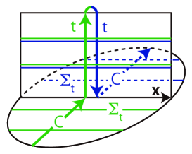
Figure 2: Same figure as Fig. 1, but with all domains of integration given in eq. (10).

III.3 Skewness from Bubble Nucleation

Now we evaluate the skewness $\langle\delta\phi^{3}(x)\rangle$ by substituting $\mathcal{L}_{\delta\phi}$ in eq. (9) to the tunneling in-in formula in eq. (10). In the following calculations, we approximate $G(x,x^{\prime})$ by that of the Bunch-Davies vacuum, by neglecting corrections due to the non-trivial part of $\mathcal{L}_{0}$ in eq. (9). This effect may affect the value of the skewness, but since it only induces a statistically homogeneous non-Gaussianity, we simply ignore it here.

The free correlation function $G(x,x^{\prime})$ of the Bunch-Davies vacuum is given by birrell-davies

$$\!\!\!\!\!\!G(x,x^{\prime})\! =\!\frac{H^{2}(\frac{1}{4}-v^{2})}{16\pi\cos\pi v}\,_{2}F_{1}\!\left[\begin{matrix}\frac{3}{2}+v,\frac{3}{2}-v\\ 2\end{matrix};\frac{1\!+\!Z(x,x^{\prime})}{2}\right],$$ (11)

where $v=\sqrt{9/4-m^{2}/H^{2}}$ and $Z(x,x^{\prime})=\cos(Hd(x,x^{\prime}))$, where $d(x,x^{\prime})$ is the geodesic distance between $x$ and $x^{\prime}$. We have $Z>1$, $Z=1$ and $Z<1$, for a timelike (imaginary $d$), null ($d=0$), and spacelike (real $d$) separation, respectively. As mentioned before, a branch of $G(x,x^{\prime})=G(Z(x,x^{\prime}))$ should be specified when $Z>1$ and it can be done by adding small imaginary part $\pm i\epsilon$ to $Z$ as $G(Z(x,x^{\prime})\pm i\epsilon)$ .

We assume $\lambda\ll 1$ to avoid possible strong coupling problems. To leading order in $\lambda$, we obtain

$$\Big{<}\delta\phi^{3}(x)\Big{>} =-i\lambda H^{-3}\int_{C}\mathrm{d}\tau^{\prime}\int_{0}^{\pi}\mathrm{d}\chi^{\prime}\int\mathrm{d}\Omega^{\prime}$$

$$\times \sin^{3}\chi^{\prime}\sinh^{2}\tau^{\prime}\,\delta\left(\chi^{\prime}-HR_{\rm W}\right)\left(G(x,x^{\prime})\right)^{3}\,.$$ (12)

where

$$C:\ -i\,\frac{\pi}{2}\to 0-i\,\epsilon\to\infty\to 0+i\,\epsilon\to i\,\frac{\pi}{2}\,,$$ (13)

as shown in Fig. 3. Among the domains of integral, $\tau^{\prime}\in(-i\,\pi/2,+i\,\pi/2)$ and $\tau^{\prime}\in(0\pm i\,\epsilon,\infty)$ correspond to the E- and C-regions, respectively. Integration in the R- or L-regions is unnecessary because $\mathcal{L}_{I}$ vanishes there. A small imaginary part in $\tau^{\prime}\in(0\pm i\epsilon,\infty)$ gives a small imaginary part to $Z(x,x^{\prime})$ to select the Feynman or anti-Feynman propagator.

Evaluation of eq. (12) is straightforward in principle, but it is significantly simplified if we use the O(4)-symmetry of the $N$-point functions in the tunneling in-in formalism. Just for illustration, let us consider the case when $x$ is in the R-region. In this case, computing $\langle\delta\phi^{3}(x)\rangle$ at $r_{\mathrm{R}}=0$, where integration over $\chi$ and $\Omega$ is trivial, is enough since the value at any other point in the R-region can be known from the O(4)-symmetry.

After integrating over $\chi$ and $\Omega$, the integration over $\tau$ along $C$ remains. Since the original path $C$ passes near the singularity, it makes the integral difficult to evaluate numerically. To avoid it, we deform the path $C$ to another path $C^{\prime}$ without crossing the branch cut or the poles of the integrand as in Fig. 3. The resulting $\langle\delta\phi^{3}(x)\rangle$ is obtained in terms of the open-slice coordinates, but the expression in terms of the flat-slice coordinates can be easily found by the coordinate transformation.

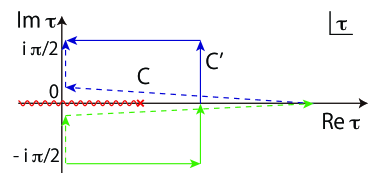
Figure 3: The structure of integrand and integration path in eq. (12). The wavy line is the branch cut, the dotted line is the original path $C$, while the solid line is a detoured path $C^{\prime}$ used for numerical evaluation.

Fig. 4 shows the skewness on flat slices at time $t$ as a function of the radial coordinate $r$, $\langle\delta\phi^{3}(r,t)\rangle/\langle\delta\phi^{3}(0,t)\rangle$, for $Ht=50$ and $HR_{\rm W}=0.2\pi$ for several values of $m/H$. To see the dependence of the skewness on the model parameters, we introduce a normalized skewness $F(t)$ at the center of the bubble by

$$\langle\delta\phi^{3}(0,t)\rangle=4\pi\lambda\,\sin^{3}(HR_{\rm W})\left(\frac{3H^{2}}{8\pi^{2}m^{2}}\right)^{3}H^{3}F(t)\,.$$ (14)

The result is shown in Fig. 5. From this, we see that $F\approx e^{-\frac{m^{2}}{H^{2}}Ht}$.

We see that the skewness is large inside the bubble and it decreases as one moves away from the bubble, and its radial dependence is stronger for larger $m/H$. These features can be understood from the fact that $G(x,x^{\prime})$ is roughly given by $(3H^{4}/8\pi^{2}m^{2})|1-Z|^{-m^{2}/(3H^{2})}$ for $m/H\ll 1$ and $Z$ is not very close to 1. The apparent divergent behavior at the bubble wall comes from the UV divergence in $G(x,x^{\prime})$. But, this divergence disappears as soon as the finite resolution of observations or renormalization of the theory is taken into account.

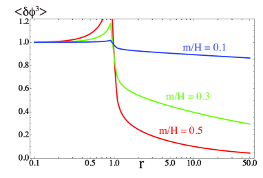
Figure 4: $\langle\delta\phi^{3}(r,t)\rangle$ normalized by the value at the center as a function of $r$ at $Ht=50$.

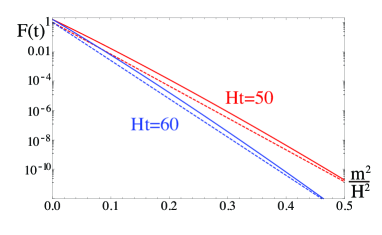
Figure 5: A normalized skewness as a function of time, $F(t)$. The solid lines are the result of numerical evaluation and the dashed lines are analytical approximation, $e^{-\frac{m^{2}}{H^{2}}Ht}$.

IV Non-Gaussian Bubbles in the Sky

Now we study signatures of our model in the CMB anisotropy. In our model, the evolution of the universe after the inflaton and the tunneling field decay, is exactly the same as the ordinary curvaton scenario Lyth:2002my . Here, we estimate the curvature perturbation after the curvaton decay by using the sudden-decay approximation Sasaki:2006kq .

After inflation the curvaton starts to roll down the potential and undergoes damped oscillations when the Hubble parameter becomes smaller than $m$. The curvaton energy density behaves like a pressureless matter during this stage of damped oscillations. At the time $t=t_{\mathrm{curv}}$ when the curvatons decay, the energy density of the universe consists of that of radiation $\rho_{r}$ generated from the decay of the inflatons and that of the curvaton $\rho_{\phi}$. The contribution of each component to the total curvature perturbation of the universe may be conveniently expressed in terms of $\zeta_{r}$ and $\zeta_{\phi}$, which are defined as the curvature perturbations on the uniform energy density slices of the radiation and the curvaton, respectively.

It is known that each of them is separately conserved on superhorizon scales at $t<t_{\mathrm{curv}}$. As for $\zeta_{\phi}$, it may be evaluated by the energy density fluctuations on the uniform inflaton field slice at the end of inflation, $\delta\rho_{\phi}/\rho_{\phi}$, as

$$\zeta_{\phi}=\frac{1}{3}\left.\frac{\delta\rho_{\phi}}{\rho_{\phi}}\right|_{t_{\rm e}}=\frac{1}{3}\left.\left(2\,\frac{\delta\phi}{\phi_{0}}+\frac{\delta\phi^{2}}{\phi_{0}^{2}}\right)\right|_{t_{\rm e}},$$ (15)

where $t_{\rm e}$ is the time at the end of inflation.

After the curvaton decay, the total curvature perturbation on the slices of uniform total energy density, $\zeta$, is conserved on superhorizon scales. It is given by

$$\zeta=(1-r_{\phi})\zeta_{r}+r_{\phi}\zeta_{\phi}\,,$$ (16)

where $r_{\phi}=3\rho_{\phi}/(4\rho_{r}+3\rho_{\phi})|_{t_{\rm curv}}$.

For the moment, we ignore the contribution from $\delta\phi^{2}/\phi_{0}^{2}$ and concentrate on the skewness generated by the nonlinear interaction with the tunneling field. Then we have

$$\langle\zeta^{3}(r)\rangle\approx r_{\phi}^{3}\langle\zeta_{\phi}^{3}(r,t_{\mathrm{e}})\rangle\approx\frac{8}{27}r_{\phi}^{3}\frac{\langle\delta\phi^{3}(r,t_{\mathrm{e}})\rangle}{\phi_{0}^{3}}\,,$$ (17)

where $\langle\delta\phi^{3}\rangle$ is given by Eq. (12). An important feature is that the skewness of the curvature perturbation depends on the position of the bubble due to the spatial dependence of $\langle\delta\phi^{3}\rangle$.

To proceed, we focus only on the large angular scale CMB anisotropy for which the Sachs-Wolfe effect dominates. In this regime, the CMB temperature anisotropy can be written in terms of the curvature perturbation as $(\delta T/T)(\hat{\bm{n}})=(1/5)\,\zeta({\bm{x}}_{0}+r_{*}\hat{\bm{n}},t_{*})$ , where ${\bm{x}}_{0}$ is the comoving position of the observer measured from the bubble center, $\hat{\bm{n}}=(\sin\theta\cos\varphi,\sin\theta\sin\varphi,\cos\theta)$ is the directional cosine of the sky seen by the observer, $r_{*}$ is the comoving distance from the observer to the last scattering surface and $t_{*}$ is the time at the last scattering surface. Then, defining the non-Gaussianity parameter $f_{\rm NL}$ as $(3/5)f_{\rm NL}(\hat{\bm{n}})\equiv\langle\zeta^{3}({\bm{x}}_{O}+r_{*}\hat{\bm{n}},t_{*})\rangle/\langle\zeta^{2}\rangle^{2}$, we have

$$f_{\rm NL}(\hat{\bm{n}})\approx\frac{40r_{\phi}^{3}}{81\langle\zeta^{2}\rangle^{2}}\frac{\langle\delta\phi^{3}(|{\bm{x}}_{O}+r_{*}\hat{\bm{n}}|,t_{*})\rangle}{\phi_{0}^{3}}\,.$$ (18)

One explicitly sees that the dependence on the position of the bubble center breaks the statistical isotropy.

For completeness, let us discuss the additional contributions to $f_{\rm NL}$ which we have ignored. The contribution of $\zeta_{r}$ to non-Gaussianity is known to be very small as long as the vacuum is in the Bunch-Davies vacuum Maldacena:2002vr . A deviation from the Bunch-Davies vacuum may give rise to a non-zero non-Gaussianity. It is expected to be statistically homogeneous and isotropic but scale-dependent (in the Fourier space). It may be detected by the templates of the equilateral or orthogonal types. The contribution from the part of $\zeta_{\phi}$ quadratic in $\delta\phi/\phi_{0}$ gives rise to a local type non-Gaussianity which is again statistically homogeneous and isotropic, and which may be detected by the squeezed type templates.

This contribution from the nonlinearity of $\delta\phi/\phi_{0}$ in $\zeta_{\phi}$ may be estimated as follows. Roughly speaking, $\langle\delta\phi^{4}\rangle\approx\langle\delta\phi^{2}\rangle^{2}\approx(H/2\pi)^{4}$ for $m/H\ll 1$, and the contribution to $\langle\zeta_{\phi}^{3}\rangle$ is about $(4/9)(H/2\pi\phi_{0})^{4}$. Thus, the condition that $f_{\rm NL}$ is dominated by the nonlinear interaction with the bubble is given as

$$\frac{4}{9}\left(\frac{H}{2\pi\phi_{0}}\right)^{4}\ll\frac{32\pi}{27}\lambda\,\sin^{3}(HR_{\rm W})\left(\frac{3H^{2}H}{8\pi^{2}m^{2}\phi_{0}}\right)^{3}F(t_{\mathrm{e}})\,.$$

This is satisfied in an example we compute below.

For illustration, we plot $f_{\rm NL}(\hat{\bm{n}})$ in the CMB sky in Fig. 6. The parameters are $m/H=0.3$, $HR_{\rm W}=0.2\pi$ $H/\phi_{0}=0.001$ $\lambda=0.005$, $r_{\phi}=0.1$, $|{\bm{x}}_{0}|=r_{*}=2$, $Ht_{\mathrm{e}}=50$. For the variance $\langle\zeta^{2}\rangle$ we simply impose the observational result, $\langle\zeta^{2}\rangle=A_{\zeta}^{2}\equiv 6.25\times 10^{-10}$ Komatsu:2010fb , assuming that it is dominated by $\zeta_{r}$. Since $\langle\delta\phi^{2}\rangle\approx(H/2\pi)^{2}$ when $m/H\ll 1$, this assumption is justified if $(2r_{\phi}/3)^{2}(H/2\pi\phi_{0})^{2}\ll A_{\zeta}^{2}$, which is marginally satisfied in the above example.

The typical value of $f_{\rm NL}$ at the center of the bubble when the parameters satisfy the above conditions is estimated as

$$f_{\rm NL}^{\mathrm{(cen)}}\!\approx\frac{3\!\times\!10^{-4}\,\lambda\,r_{\phi}^{3}\,\sin^{3}(\!HR_{\rm W}\!)}{A_{\zeta}^{4}\,\exp\left({(\frac{m}{H})^{2}Ht_{\mathrm{e}}}\right)}\left(\!\frac{H}{m}\!\right)^{\!6}\!\left(\!\frac{H}{\phi_{0}}\!\right)^{\!3}\!\!\,.$$ (19)

This gives $f_{\rm NL}^{\mathrm{(cen)}}\approx 15$ for the parameters given above and agrees with the result in Fig. 6 within the errors shown in Fig. 5. From this estimation, we find that the resultant $f_{\rm NL}$ is rather sensitive to the values of $m/H$ and $H/\phi_{0}$. It is enhanced for smaller $m/H$ and larger $H/\phi_{0}$.

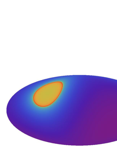
Figure 6: Non-Gaussianity map in the CMB sky, for the model parameters given in the text. Colors correspond to the values of $f_{\rm NL}$.

V Conclusion

In this paper, we calculated the skewness in the CMB temperature anisotropy in a model with bubble nucleation during inflation, motivated by the string theory landscape. We considered bubble nucleation in the curvaton scenario of inflation in which the curvaton vacuum fluctuations are affected by the bubble nucleation through interaction with the tunneling field. The calculation was done by extending the in-in formalism to the instanton background preparation . We found that there can be spatially localized, bubble-shaped skewness which is large inside the bubble.

As far as we know, bubble-shaped non-Gaussianities have not been studied carefully yet in observation. So it seems interesting to look for such a non-Gaussianity already in the current observational data. As pointed out by Komatsu and Spergel Komatsu:2001rj , the bispectrum, corresponding to the 3-point function, contains much more information than the single value of the skewness. Thus, analysis beyond skewness may improve the observability of bubble-shaped non-Gaussianities. We hope to come back to this issue in a future publication.

Since the string theory landscape gives a strong motivation for inflation models with bubble nucleation, studies of such inflation models may be regarded as testing string theory using the universe as a laboratory. In any case, if any signature of bubble nucleation during inflation is found in observation, it gives a huge impact on the physics of the early universe, including string theory.

Finally, we note that in the evaluation of the skewness we neglected the effect of deviations from the Bunch-Davies vacuum. This may affect details of our result, though generic features are expected to remain the same. This effect can be evaluated by studying the evolution of mode function on the instanton background Yamamoto:1996qq . We plan to come back to this issue in the near future.

- (1) Kachru S., Kallosh R., Linde A. D. and Trivedi S. P., Phys. Rev.D, 68 (2003) 046005; Kachru S. et al., JCAP, 0310 (2003) 013.
- (2) Susskind L., arXiv:hep-th/0302219 (2003); Freivogel B., Kleban M., Rodriguez Martinez M. and Susskind L., JHEP, 03 (2006) 039.
- (3) Yamamoto K., Sasaki M. and Tanaka T., Phys. Rev.D, 54 (1996) 5031.
- (4) Yamauchi D., Linde A., Naruko A., Sasaki M. and Tanaka T., Phys.Rev.D, 84 (2011) 043513.
- (5) Coleman S. R. and De Luccia F., Phys. Rev.D, 21 (1980) 3305.
- (6) Sugimura K., Yamauchi D. and Sasaki M., JCAP, 1201 (2012) 027; Aguirre A., Johnson M.C. and Larfors M., Phys. Rev. D, 81 (2010) 043527.
- (7) Komatsu E. et al., Astrophys. J. Supp., 192 (2011) 18.
- (8) Maldacena J. M., JHEP, 0305 (2003) 013.
- (9) Komatsu E. and Spergel D. N., Phys. Rev.D, 63 (2001) 063002.
- (10) Creminelli P., Nicolis A., Senatore L., Tegmark M. and Zaldarriaga M., JCAP, 0605 (2006) 004.
- (11) Senatore L., Smith K. M. and Zaldarriaga M., JCAP, 1001 (2010) 028.
- (12) Lyth D. H., Ungarelli C. and Wands D., Phys.Rev.D, 67 (2003) 023503; Enqvist K. and Sloth M.S., Nucl.Phys.B, 626 (2002) 395; Moroi T. and Takahashi T., Phys.Lett.B, 522 (2001) 215; Mazumdar A. and Rocher J., Phys.Rept., 497 (2011) 85.
- (13) Sasaki M., Valiviita J. and Wands D., Phys.Rev.D, 74 (2006) 103003.
- (14) Birrell N. D. and Davies P. C., Quantum fields in curved space (Cambridge University Press) 1982.
- (15) Tanaka T., Sasaki M. and Yamamoto K., Phys. Rev.D, 49 (1994) 1039.
- (16) Yamamoto K., Prog. Theor. Phys., 91 (1994) 437.
- (17) Sugimura K. et al., in preparation.
- (18) Park D. S., JHEP, 1201 (2012) 165.