Mesoscopic Model for Free Energy Landscape Analysis of DNA sequences.

Abstract

A mesoscopic model which allows us to identify and quantify the strength of binding sites in DNA sequences is proposed. The model is based on the Peyrard-Bishop-Dauxois model for the DNA chain coupled to a Brownian particle which explores the sequence interacting more importantly with open base pairs of the DNA chain. We apply the model to promoter sequences of different organisms. The free energy landscape obtained for these promoters shows a complex structure that is strongly connected to their biological behavior. The analysis method used is able to quantify free energy differences of sites within genome sequences.

I Introduction

The study of biomolecules at a mesoscopic level tries to identify the main degrees of freedom of the system and understand its behavior in terms of the dynamical and statistical-mechanics properties of the model. At this level, the concept of a free-energy landscape (FEL) represents a paradigm for the comprehension of several biological complex problems such as protein folding, protein structure, and biomolecular interaction  Wales . A FEL gives the change in the free energy of a system when the different degrees of freedom change. The description given by the topology of the FEL permits to connect structure, dynamics, and thermodynamics in many different systems ranging from atomic clusters to biomolecules or soft matter systems  Wales2 .

Here we address our attention to the characterization of the FEL of DNA sequences and, in particular, those sites with regulatory and transcriptional relevance. Recently, a great attention has been devoted to the mechanism whereby proteins bind to specific sites on DNA search . The quantification, grounded in a physical basis, of the strength of these binding sites is an open problem. In this paper, we propose a model which allows us to calculate free energy differences between specific and nonspecific binding sites. Even more, we are able to build, from the trajectories of the model, a representation of the free energy landscape.

The model is inspired in the protein search of the binding sites in a DNA chain. This search is a combination of three-dimensional (3D) jumps between separated regions of DNA and one-dimensional (1D) diffusion along the chain. It has been stated that most of the search time is spent in the 1D diffusion process since the time jumps in three dimensions is negligible PhysicsMolBio ; Berg ; Marko . Thus, the restriction to a 1D search is a good starting point for our model. On the other hand, it has also been conjectured that the dynamics of the DNA chain plays an important role in the recognition of binding sites by the regulatory factors or the transcription protein Kalosakas04 ; Apostolaki11 . Thus, transcription processes, for instance, would be induced by the binding of RNA-polymerase to openings (bubbles) in the DNA chain. This idea is supported by computational approaches to the DNA dynamics Alexandrov_PLoSCB , and experimental evidences expDNA . Our model follows this idea and considers the interaction of a test particle, which explores the DNA chain, coupled to the bubbles. In order to be physically and biologically relevant, such a description should provide useful qualitative and quantitative information about the process. A similar strategy has been used to characterize complex networks and identify regions of special relevance (communities). In such an approach, a “fictitious” Brownian particle goes over the graph PNASnet and its dynamics reveals “thermodynamics” and structural quantities of the topology JGG .

In this paper, we propose a mesoscopic model for DNA-particle interaction. In our picture, the test particle undergoes a 1D Brownian motion in interaction with a classical field, the DNA chain itself, whose dynamics is also affected by the presence of the particle. The test particle interacts more strongly with open base-pairs of the DNA chain. In this way “softer” regions of the DNA sequence are more likely to be visited by the particle, which will help also in stabilizing the bubbles. This interaction is not sequence-dependent, as the DNA base-pair dynamics already depends on the sequence. Thus, this model could also represent the interaction of a real protein as RNA-polymerase, with the DNA bubbles.

Particle and chain are described at the same level of complexity. We use the Peyrard-Bishop-Dauxois (PBD) PBD ; Peyrard_NonL model to perform the dynamics of the chain. This model was proposed initially for the study of DNA thermal denaturation and incorporates the formation and dynamics of bubbles in a natural way. The PBD model can take into account the sequence information through its parameters.

Our model incorporates three basic ingredients of the physics of the system: DNA sequence, bubble dynamics, and 1D particle diffusion. The analysis of the DNA-particle complex allows us not only to identify possible binding sites, but also to describe the whole structure of the free-energy landscape and determine free-energy differences between different representative states. We show the validity and usefulness of our approach by studying the FEL of three promoter sequences. In each case, the FEL topology gives insight into the biological behavior of the system.

II Model

We describe the DNA chain by a modified Peyrard-Bishop-Dauxois modelPBD ; Peyrard_NonL ; RTR10 . There, the complexity of the DNA molecule is reduced to the study of the dynamics of $N$ base pairs described by the variables $y_{n}$ defining the distance between the bases. In this framework $H_{DNA}=\sum_{n=1}^{N}\left[\frac{p_{n}^{2}}{2m}+V(y_{n})+W(y_{n},y_{n-1})\right]$. In our model

$$V(y)=D({\rm e}^{-\alpha y}-1)^{2}+G{\rm e}^{-(y-y_{0})^{2}/b},$$ (1)

where the first term accounts for the hydrogen bond interaction and the second one for interactions with the solvent Weber ; RTR10 . It was shown in RTR10 that the inclusion of this barrier modifies drastically the duration and stability of the bubbles.

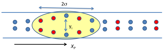
Figure 1: (Color online) Schematic illustration of the DNA-particle interaction model. The unidimensional chain (solid circles) is represented by the base pair opening coordinate ($y_{i}$) while the probe particle (shaded ellipse) is a diffusing particle along the DNA chain ($X_{p}$).

The potential $W(y_{n},y_{n-1})$ describes the stacking interaction between the base pairs along the DNA strand,

$$W(y_{n},y_{n-1})=\frac{1}{2}K\left(1+\rho e^{-\delta(y_{n}+y_{n-1})}\right)(y_{n}-y_{n-1})^{2}.$$ (2)

In order to study different DNA sequences, the PBD model includes sequence dependent Morse parameters: $D_{n}$, $\alpha_{n}$. Regarding the DNA chain, we use the set of parameters param considered in RTR10 .

The particle is represented by a Brownian particle (see Fig. 1) moving in a one-dimensional space with coordinate $X_{p}$ and interacting with the DNA chain through a phenomenological potential which depends on $X_{p}$ and the set of coordinates $\{y_{i}\}_{i=1}^{N}$: $H_{P}=p_{p}^{2}/2m_{p}+V_{int}(X_{p},\{y_{i}\})$ with

$$V_{int}(X_{p},\{y_{i}\})=-\frac{B}{\sqrt{\pi\sigma^{2}}}\sum_{i}\tanh(\gamma y_{i})\ e^{-(X_{p}-ia)^{2}/\sigma^{2}}$$ (3)

where $B$ sets the interaction amplitude, $\gamma$ the range of interaction with the base separation and $\sigma$ the spatial range of interaction on the DNA chain. The functional form for the interaction has been chosen to be linear at low $y_{i}$ and to saturate at large $y_{i}$ in order to avoid that the chain opens indefinitely. Note that with this term the particle is trying to open the chain in a length range of $\sigma$ and get self-trapped. Although possible, no sequence dependence is included in this term since we are interested in giving a general picture of the FEL.

We still have to fix the parameters for this interaction term. For the particle damping and mass, we take $\eta_{p}=10^{14}s^{-1}$ and $m_{P}=7000Da$. These values are of the order of magnitude of proteins which bind DNA hop ; biol . The intensity of the interaction chosen is $B=0.52eV$. This value provides local interactions of the order of the Morse potential dissociation energy at each base pair. The parameter $\gamma=0.8\AA^{-1}$ saturates the interaction at $y=1.25\AA$, a typical value for open base pairs. We take $a=1$ for the longitudinal separation between base pairs, in arbitrary units, and consider $\sigma=3$. This provides an interaction range of around $5$ or $6$ base pairs (bp). It is interesting to note that this value has been chosen in order to observe states with bubbles of $10-20$ bp, which is an adequate width for the processes we take into account here arkiv .

Once we have fixed the model parameters, we derive the Langevin equations for both the chain bases and the particle. For the chain, we get:

$$m\frac{\partial^{2}y_{n}}{\partial t^{2}}+m\eta\frac{\partial y_{n}}{\partial t} = -\frac{\partial\left[W(y_{n},y_{n+1}+W(y_{n-1},y_{m})\right]}{\partial y_{n}}$$ (4)

$$-\frac{\partial V}{\partial y_{n}}-\frac{\partial V_{int}}{\partial y_{n}}+\xi_{n}(t),$$

where $\eta$ stands for the damping and $\xi_{n}$ for the thermal noise, so $\langle\xi_{n}(t)\rangle=0$ and $\langle\xi_{n}(t)\xi_{k}(t^{\prime})\rangle=2m\eta k_{B}T\delta_{nk}\delta(t-t^{\prime})$ hold.

The Langevin equation for the particle is:

$$m_{p}\frac{\partial^{2}X_{p}}{\partial t^{2}}+m_{p}\eta_{p}\frac{\partial X_{p}}{\partial t}=-\frac{\partial V_{int}}{\partial X_{p}}+\xi_{p}(t).$$ (5)

where, $\eta_{p}$ stands for the particle damping and $\xi_{p}$ for the thermal noise. The fluctuation-dissipation relation reads as $\langle\xi_{p}(t)\rangle=0$ and $\langle\xi_{p}(t)\xi_{p}(t^{\prime})\rangle=2m_{p}\eta_{p}k_{B}T\delta(t-t^{\prime})$.

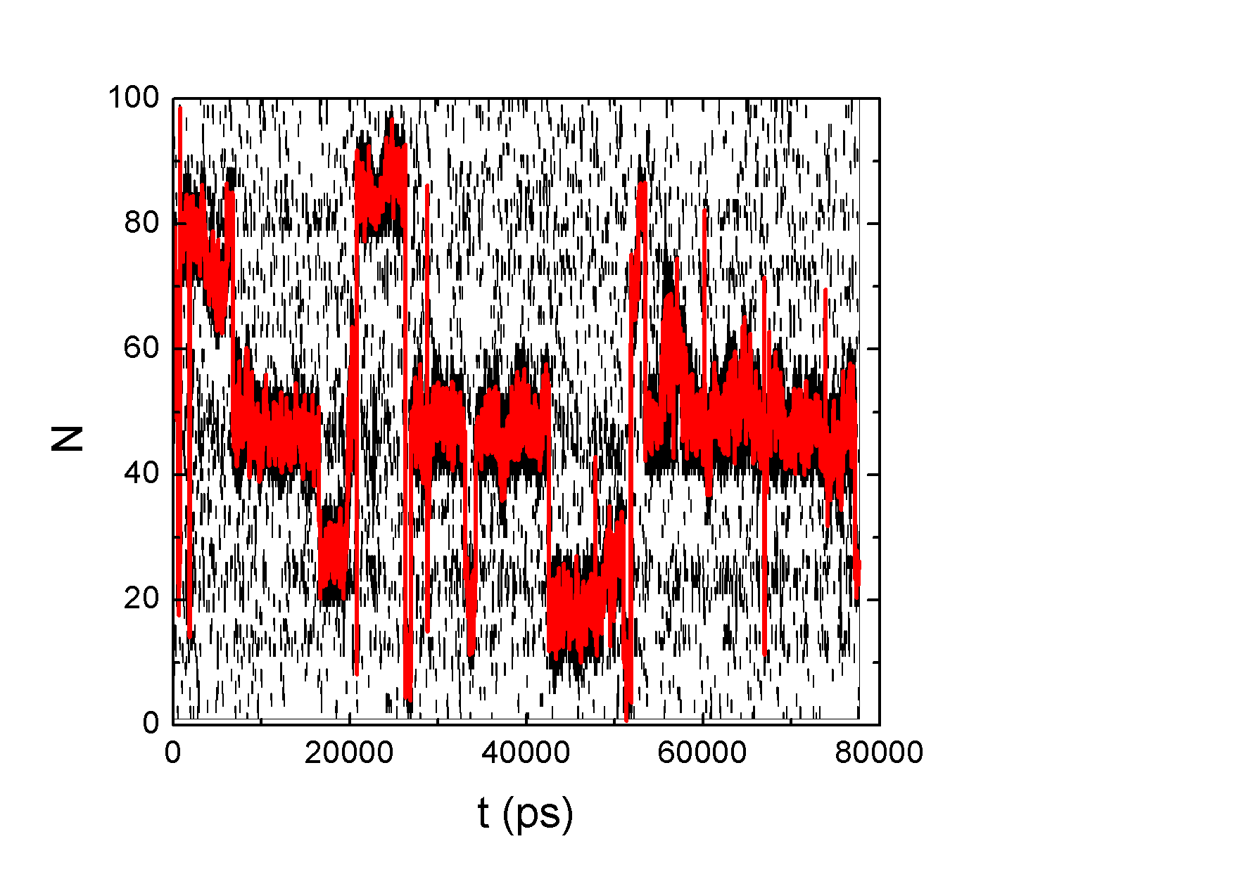
Figure 2: (Color online) Trajectory of the particle shown in red line (light gray) with the DNA chain for a collagen sequence (see results section). Black points stands for open bp ($y_{AT}>1.\AA$ or $y_{CG}>1.5\AA$) and white for closed ones.

The equations were numerically integrated using the stochastic Runge-Kutta algorithm sde2 . The integration of the Langevin equations of motion provides trajectories of the particle and the DNA chain. Each DNA sequence was simulated in five different realizations for $40\mu s$, using $10$ fs time steps and a $1\mu s$ preheating time. Since it has been reported that 1D diffusion periods cover a time of the order of milliseconds hop ; biol , the simulation time used is reasonable for the problem considered here. The simulation temperature is $T=290K$ and the boundary conditions for the protein are periodic, while for the chain we consider the hard boundary conditions discussed in RTR10 . An example of such a trajectory is given in Fig. 2. It is observed that the particle moves in a “sea” of open bubbles which clearly shows the soft domains of the genome structure. The particle eventually jumps between these domains opening large stable bubbles. As seen in the figure the dynamics of the bases is strongly affected by the presence of the particle.

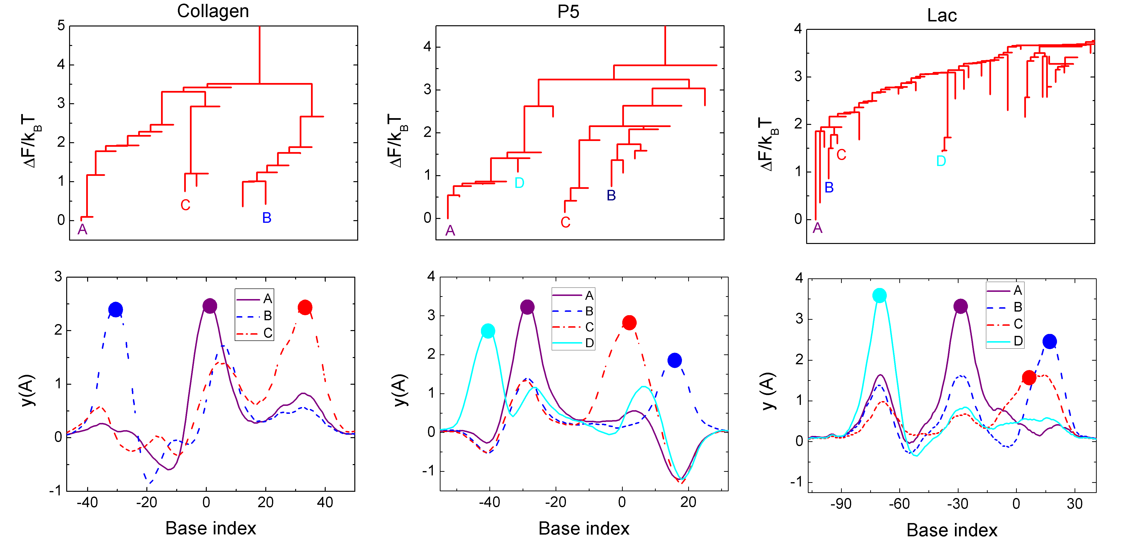
Figure 3: (Color online) Free energy dendrograms (top) for each of the three sequences together with selected states (bottom). The dendrograms represented are a detail of the whole structure showing low energy basins only. The construction of the dendrogram has been performed considering the representative node of each basin. Significant biological states have been searched within the network structure. They correspond to the important basins of the hierarchical free energy organization.

III Analysis

To extract useful information of such trajectories, and due to the large dimensionality of the system, we apply the principal component analysis (PCA) jolliffe_book to the chain trajectory. It has been proved RTR10 that the first few eigenvectors unveil the softest regions of the DNA chain and hence the possible binding sites for our particle. Even more, PCA reduces the large number of degrees of freedom of the system to just a few, by projecting the coordinates of the system into the first few eigenspaces (reduced trajectories). For each of the sequences considered, we restrict ourselves to the first five eigenspaces. This subspace accounts for $75\%$ of the total fluctuations of the chain dynamics.

To obtain the FEL properties of the system we make use of the map of trajectories to a conformational Markov network (CMN) [17,20]. The CMN has been proven to be a useful representation of large stochastic trajectories rao ; caflisch ; gfeller . This coarse grained picture is usually constructed by discretizing the conformational space explored by the dynamical system and considering the hops between the different configurations as dictated by the MD simulation. In this way, the nodes of a CMN are the subsets of configurations defined by the conformational space discretization, and the links between nodes account for the observed transitions between them. The information of the stochastic trajectory allows us to assign probabilities for the occupation of a node ($P_{i}$) and for the transitions between two different configurations ($P_{ij}$). Defined as above, a CMN is thus a weighted and directed graph. It should be stressed that the information contained in the CMN is much richer that one given by equilibrium statistical mechanics since it includes the dynamics of the system encoded in the probability transitions, $P_{ij}$.

In our case, we start from the reduced trajectory for the DNA (obtained using five principal components) and the trajectory of the test particle. We discretize the total coordinate space in 20 bins of equal volume for the reduced trajectory and $N$ bins (the DNA base pairs) for the particle. This will constitute the microstate space of the CMN, each node with occupancy probability $P_{i}$ obtained from the reduced trajectory. Once the CMN has been built, we split it into basins of attraction, i.e., regions in which the probability fluxes ($P_{ij}$) converge to a common state (attractor) of the network. This task is usually hard, since algorithms scale as power law of the system size. In this case we have applied the stochastic steepest descent algorithm developed in PLoSDPG , which scale as $N\log N$. In this decomposition, a basin corresponds to a coarse-grained state (of connected nodes) of the CMN. In next section, we represent each basin by its attracting node.

Once these basins have been defined we can represent the FEL by a hierarchical tree diagram (dendrogram) PLoSDPG , built according to the weights and links among the basins. This representation is similar to the “disconnectivity graph” scheme used in other context Wales ; Wales2 ; krivov . First, an “adimensional free energy” is assigned to each node $i$ given by $F_{i}/kT=log(P_{w})-log(P_{i})$ where $w$ represents the weightiest node. Using this magnitude as control parameter, we slowly increase it step by step from its zero initial value. At each step of this process, we obtain a network composed of those nodes with free energy lower than the current threshold value. As the free-energy threshold increases, new nodes emerge together with their links. These new nodes may be attached to any of the nodes already present in the network or they can emerge as a disconnected component. At a certain value of $F/kT$, some components of the network become connected by the links of a new node incorporated at this step. Initially we have a set of disconnected vertical lines (corresponding to basins) which become linked once the control parameter has overcome the barriers between them i. e. when the free energy of the saddle nodes is reached. Then we draw a horizontal line linking these two basins. Obviously, for large threshold all the network is connected. We can plot this process as a “tree diagram” or dendrogram.

Using this representation we can understand qualitatively and quantitatively the hierarchical organization of the basins and the barriers among them and figure out the behavior of different sequences.

This method could be applied to a DNA chain without a particle. However, the inclusion of the particle is essential to get the FEL of the system. An analysis of the DNA alone (PBD model) lets us determine the opening probabilities and average position of the chain base pairs, and unveils the softer regions that can indeed be related to sites of biological importance. Nevertheless, the FEL of this model is trivial, as opening events are rare and the chain remains closed for most of the time. The inclusion of the particle stabilizes the bubbles (as can be observed in Fig. 2) and allows us to go further in terms of predictions. We are able to define relevant states in a precise and systematic way (basins), to predict possible binding sites, and to extract the thermodynamical magnitudes related with them, thus characterizing these sites in terms of biological importance.

IV Results

To illustrate the method and validate our model, we analyze three different promoter sequences. Promoters are DNA regions in which regulation and initiation of transcription of a gene occurs. Two of them correspond to the so called strong promoters, while the one left is a weak promoter weak_book . Strong promoters show a high level of expression in mRNA and usually their sequences are close to the consensus sequence. The strong promoters studied here are the P5 virus promoter, given by the 69 bp sequence shown in Kalosakas04 and the human collagen type I $\alpha 2$ chain, given by the 80 bp sequence shown in Alexandrov_PLoSCB . Finally, the weak promoter is the lac operon regulatory region, whose 129 bp sequence has been taken from Apostolaki11 .

In Fig. 3 (top) we show a detail of the free energy dendrograms for each of the mentioned sequences. The basin structure consists of a big set of low occupied (high energy) basins, and a small set which gathers almost the whole trajectory (see below). This small set of basins is the one shown in Fig. 3.

In the botton of Fig. 3 some remarkable states for each of the three promoters are highlighted. The method identifies states with a biological meaning as they correspond to the most important basins. The most significant sites we are dealing with are the transcription starting site (TSS) and the TATA box, although additional promoter sequences can be found depending on the genome. The RNA polymerase binds to the TSS, starting the transcription into mRNA. Promoter sequences are usually labeled from the TSS ($+1$). The TATA-box is found approximately $35$ base pairs upstream from the TSS weak_book .

For the collagen chain, three states have been highlighted. State A identifies the TSS, showing a bubble in this region with the particle placed just there. States B and C are linked to excitations of other important sites such as the TATA box (state B), see Alexandrov_PLoSCB . In the same way, we have found a basin related to the TSS in the case of the P5 chain (state C) and the lac operon (state C), together with other regulatory sites.

The arrangement of these basins in the free energy dendrogram informs about the relative free energy between the states and the relation between them. For example, the collagen dendrogram contains three main branches, each one related to each of the three states shown. The P5 promoter shows an analogous structure: two main branches and another one divided into two states (B and C) which are kinetically close. The remaining states of each branch correspond to states similar to that shown, with only slight variations in the chain conformation or in the particle position.

The lac promoter shows a clearly different behavior compared with the two strong promoters. From a qualitative point of view, the arrangement of basins differs from the P5 sequence or the collagen one. To visualize quantitatively the difference, the basin occupancy is plotted in Fig. 4. We show the weight of each basin (red bars) for the three sequences together with the accumulated weight (blue line). It is remarkable, in the case of the collagen sequence, that a few basins ($25$ out of $1661$) accumulate almost the whole weight of the network (over the $99\%$). The results for the P5 promoter are completely analogous, a few basins account for most information of the dynamics. These basins are the ones shown in the dendrogram of Fig. 3. When we inspect the bottom graph in Fig. 4 we see a completely different tendency. In the lac network, the distribution of weight among the basins is more uniform.

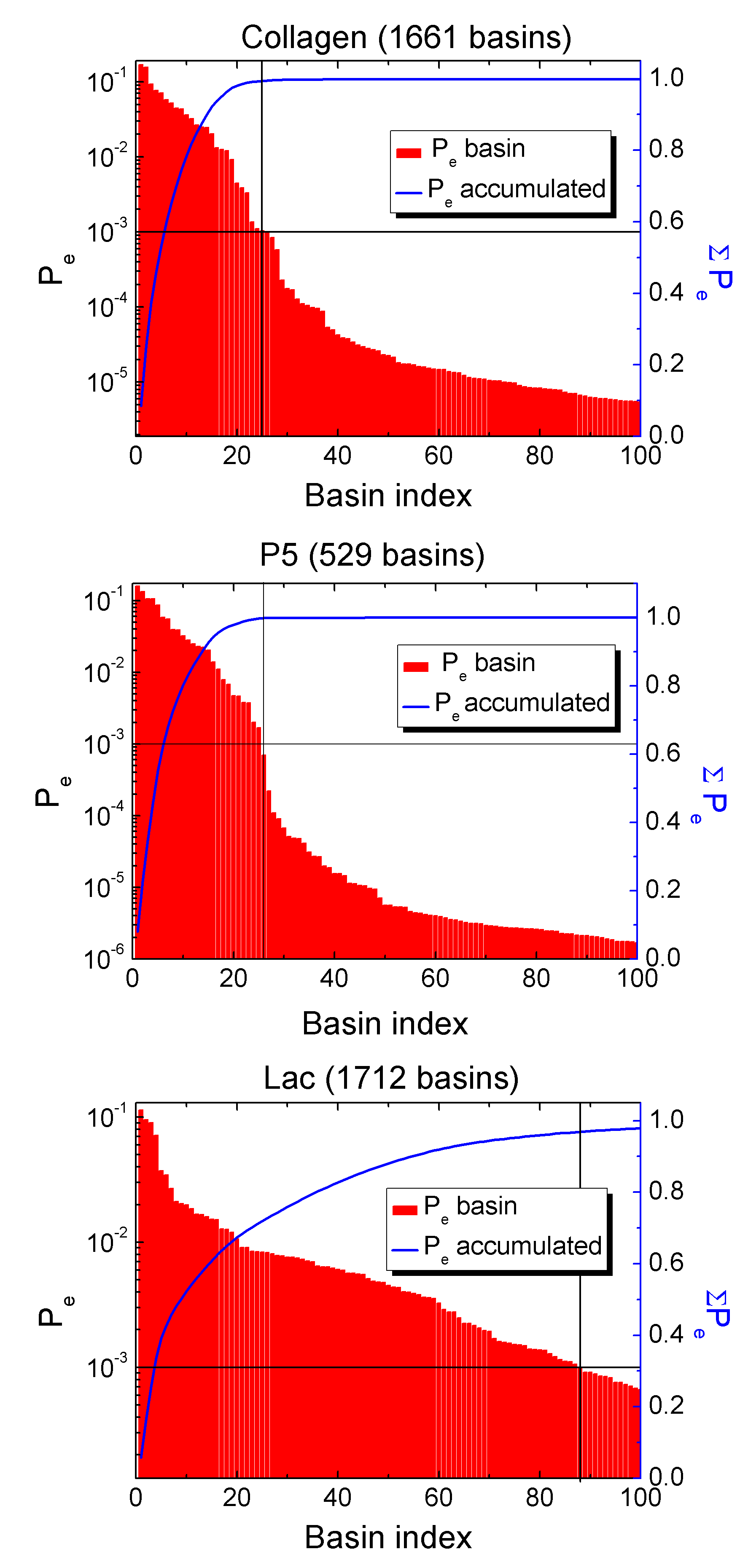
Figure 4: (Color online) Basin occupancy (bars) together with accumulated weight (solid line) for the collagen, P5 and lac sequences. The horizontal line shows the weight threshold between specific and nonspecific states. The vertical line establishes such a frontier in terms of basins. Note the logarithmic y axis.

For the collagen and P5 networks we can define a threshold from which the individual contribution to the total weight is negligible. The trajectory is concentrated in around $25$ basins and the remainder of the network can be seen as a “background”. This “background” is limited to those basins with a weight below $10^{-3}$ (horizontal lines in Fig 4). Following this criterion, we can distinguish between specific and nonspecific states. Those basins above the threshold (vertical lines in Fig. 4) may be defined as specific states (with a clear biological function) while those below the threshold may be defined as non-specific states.

For the collagen sequence, $25$ “specific” basins appear, covering $99.41\%$ of the total trajectory. The P5 and lac sequences show respectively $23$ and $88$ “specific” basins, which gather $99.38\%$ and $96.91\%$ respectively of the total network weight. Using these definitions, we are able to calculate the relative free energy between states. These magnitudes reveal the “strength” of the different sites in each promoter. It has been reported that specific binding proteins show a greater affinity for strong promoters than for weak ones Bintu05 . To quantify these differences we calculate thermodynamical properties of the most important basins. Once we have divided the network into the different basins of attraction, several statistical magnitudes can be defined from them. The weight of the basin is defined as the sum of that of the nodes belonging to the basin, i. e. for a basin $\alpha$ we have $P_{\alpha}=\sum_{i}P_{i}$ with $i\in\alpha$. In the same way the entropy of each basin can be defined as $S_{\alpha}/k_{B}=-\sum_{i}P_{i}\log P_{i}$ with $i\in\alpha$. Attending to the previous definition of the nonspecific basin, whose thermodynamical magnitudes can be computed as explained, we can calculate the free energy of each basin with respect to the nonspecific state. If $P_{\beta}$ is the weight of the non-specific basin, then the free energy difference between a basin $\alpha$ and the macrostate $\beta$ is $\Delta F_{\alpha}/k_{B}T=-\log(P_{\alpha}/P_{\beta})$. Table 1 shows significant differences between strong and weak promoters. On the one hand we observe that both the total weight and entropy of the non-specific states in the weak promoter exceed by almost an order of magnitude the ones shown for the strong promoters. On the other hand, we can see that the specific states show much higher free energy differences with respect to the nonspecific states in the case of the strong promoters than the ones shown for the lac sequence. Thus, the analysis presented here opens the way to a systematic study of promoter character within the framework of a mesoscopic model.

Promoter	State	$P_{e}\;$	$S/k_{B}\;$	$-\Delta F/kT$
Collagen	A (TSS)	0.169	1.365	3.305
	B(TATA)	0.157	1.380	3.232
	C	0.086	0.652	2.519
	NS	0.006	0.085	0.000
P5	A(TATA)	0.135	1.051	3.130
	B	0.107	0.913	2.898
	C (TSS)	0.086	0.684	2.681
	D	0.059	0.494	2.301
	NS	0.006	0.027	0.000
lac	A(TATA)	0.115	0.970	1.311
	B	0.095	0.891	1.120
	C (TSS)	0.090	0.775	1.066
	D	0.038	0.373	0.204
	NS	0.031	0.390	0.000

Table 1: Statistical (occupation probabilities) and thermodynamical (entropy and free energy differences) magnitudes calculated for the chosen states of Fig. 3 and the nonspecific states (NS), according to the criteria shown in Fig. 4.

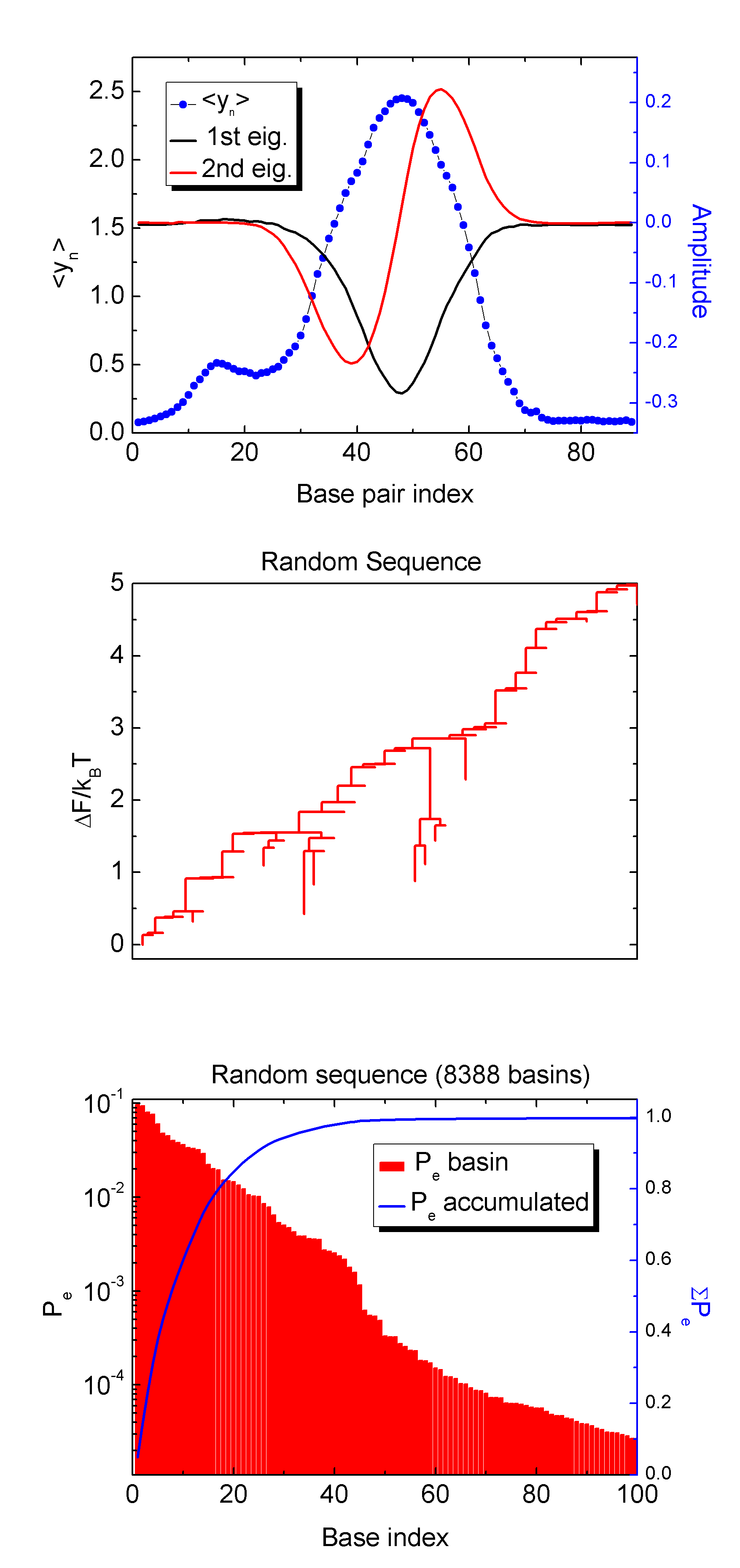
Figure 5: (Color online) Analysis of a random sequence. Top: Probability of aperture along with the first two PCA eigenvectors. Middle: Free energy dendrogram. Bottom: Basin occupancy (bars) together with accumulated weight (solid line)

In addition to the three promoter sequences of real biological systems, we have analyzed a random sequence in order to prove the validity of our model. The random sequence has been obtained by taking the P5 promoter sequence and shuffling its base pairs, so that the obtained sequence contains the same base pairs but in random positions. This sequence should contain no genetic information at all, and this fact must be reflected in our analysis.

When analyzing the random sequence with our method, we can see huge differences compared with the P5 promoter, as we would expect (see Fig. 5). First the structure of the network is completely different. As there are no prominent states in the sequence, the number of basins is huge (8388 compared with the 529 in the P5 promoter). The first two eigenvectors are representative of a homogenous lattice without localized states. The distribution of weights is also clearly different as now the “background” basins keep $6\%$ of the total network weight, an even higher value than that of the background basins gathered in the weak promoter. The dendrogram also shows a much more distributed structure where, even though some nodes appear to fall to privileged positions, their relevance within the whole network structure is far from being comparable to that shown in networks from biological promoters. All these facts validate our model, as we can clearly distinguish between a sequence with binding sites, and thus with biological information, and one with none, even though their chemical composition is the same.

V Conclusions

In this paper we have proposed and analyzed a mesoscopic model for the characterization of binding sites on DNA promoter sequences. The model is based on the 1D diffusion of an extended probe particle along the DNA chain. The particle is coupled to the opening states of the chain (bubbles). In its dynamics, it visits the main sites of the sequences, with dwelling times covering a high percentage of the trajectory. Such behavior has allowed us to perform a deep analysis of the FEL which reveals the structure of the complex phase space. The analyzed promoter sequences have been chosen to include genomes from organisms of different domains (virus, bacteria and eukaryote) and different strengths of expression. The model and the analysis used are able to capture the main biological details of the sequences.

Our model gives energy differences between specific and nonspecific sites of the promoter. Our results are in good relative agreement with some data in the literature (see for instance Bintu05 ): they account for energy ratios between weak and strong promoters. This fact would also make possible the study of sequences in which several TSSs are involved, showing the relative strength between them.

We think that our results show the power of coarse-grained or phenomenological mesoscopic models to qualitatively and quantitatively analyze complex biological systems, in particular the problem of protein-DNA regulatory and transcriptional interactions. Protein-DNA interaction is a fundamental problem which has been the object of a very intense research from many different points of view in the past years search ; Berg . Our system can be seen as the searching problem of a universal protein on a given DNA sequence, providing an approach for the study of specific protein-DNA interactions at the mesoscopic level, where different protein will interact in different ways with DNA molecules.

- (1) D. J. Wales Current Opinion in Structural Biology 20 3 10 (2010); K. Klenin, B. Strodel B, D. J. Wales , W. Wenzel Biochimica et Biophysica Acta 1814 977 1000 (2011).
- (2) D. J. Wales, Phil. Trans. R. Soc. A 370, 2877 2899, (2012).
- (3) O. Benichou et al., Phys. Rev. Lett. 103, 138102 (2009); V. Dahirel et al. Phys. Rev. Lett. 102, 228101 (2009); A. Tafvizi , L. A. Mirny, and A. M. van Oijen, ChemPhysChem 12, 1481 (2011).
- (4) K. Sneppen K. and G. Zocchi, Physics in Molecular Biology (Cambridge University Press, 2005).
- (5) P. H. von Hippel and O. G. Berg, J. Biol. Chem. 264, 675-678 (1989) .
- (6) S. E. Halford and J. F. Marko, Nucleic Acid Reseach 32 3040-3052 (2004).
- (7) G. Kalosakas, K. O. Rasmussen, A. R. Bishop, C. H. Choi, A. Usheva, Eur. Phys. Lett. 68 127 (2004).
- (8) A. Apostolaki and G. Kalosakas, Phys. Biol. 8 026006 (2011).
- (9) B. S. Alexandrov, V. Gelev, S. W. Yoo, A. R. Bishop, K. O. Rasmussen and A. Usheva PLoS Comput. Biol. 5 e1000313 (2009).
- (10) C. H. Choi et al., Nucl. Acids. Res. 32, 1584-1590 (2004); B. S. Alexandrov et al., Nucl. Acids. Res. 38, 1790 1795 (2010); S. Cuesta-Lopez et al. Nucl. Acids Res. 39 5276 5283 (2011).
- (11) M. Rosvall and C. T. Bergstrom Proc. Natl. Acad. Sci. U.S.A. 105 1118-1123 (2008).
- (12) J. Gómez-Gardeñes and V. Latora Phys. Rev. E 78 065102 (R) (2008); J-C Delvenne and A-S Libert Phys. Rev. E 83 046117 (2011).
- (13) T. Dauxois , M. Peyrard, and A. R. Bishop, Phys. Rev. E 47 684 (1993).
- (14) M. Peyrard, Nonlinearity 17 R1-R40 (2004).
- (15) R. Tapia-Rojo, J. J. Mazo and F. Falo, Phys. Rev E 82 031916 (2010).
- (16) G. Weber, Europhysics Letters 73 806-811 (2006).
- (17) eV, ; . , , . eV, , and . Da, ps-1.
- (18) M. C. DeSantis, J-L Li, Y. M. Wang, Phys. Rev. E 83 021907 (2011).
- (19) Z. Wunderlich, L. A. Mirny, Nucl. Acids. Res.86 3570 (2008).
- (20) M. Sheinman, O. Benichou, Y. Kafri and R. Voituriez. Rep. Prog. Phys. 75 026601 (2012).
- (21) H. S. Greenside and E. Helfand The Bell System Technical Journal 60 1927 (1981).
- (22) I. T. Jolliffe, Principal Components Analysis 2ed (Springer-Verlag, New York, 2002).
- (23) D. Prada-Gracia, J. Gómez-Gardeñes, P. Echenique, F. Falo, PLoS Comput. Biol. 5 e1000415 (2009).
- (24) F. Rao, A. Caflisch. J. Mol. Biol. 342 299-306 (2004).
- (25) A. Caflisch Curr. Opin. Struct. Biol. 16 71-78 (2006).
- (26) D. Gfeller, P. De Los Rios, A. Caflisch, F. Rao Proc. Natl. Acad. Sci. U.S.A. 104 1817-1822 (2007).
- (27) S. V. Krivov and M. Karplus, Proc. Natl. Acad. Sci. U.S.A. 101, 14766 (2004); S. Auer et al. Phys. Rev. Lett. 99 , 178104 (2007).
- (28) R. Schleif, Genetics and Molecular Biology (Addison-Wesley Publishing Company, 1993).
- (29) L. Bintu, N. E. Buchler, H. G. Garcia, U. Gerland, T. Hwa, J. Kondev and R. Phillips. Curr. Opin. Genetics Dev 15, 116-124 (2005).