Chapter 1 Introduction

Asteroids, also known under the now deprecated name minor planets, are a large population of small Solar System bodies which do not display cometary activity. The name asteroid, which was coined by W. Herschel in 1802, is derived from the Greek word for star-like—like stars, and unlike planets or comets, asteroids appear point-like in typical telescopic observations.

Small Solar System bodies are the most pristine material left over from the early days of the Solar System and have undergone much less processing than the planets or the Sun throughout the past . They therefore preserve crucial information on the formation and evolution of the Solar System. Asteroids, in particular, are believed to be remnant building material of the inner planets. Impacts of asteroids and comets have significantly resurfaced the terrestrial planets and their satellites and may have been a significant source of water on Earth (see, e.g., Martin2006, for a recent review). Meteorites, the remnants of Earth impactors, are the major source of extra-terrestrial material available for laboratory studies; studies of meteorites and asteroids, the parent bodies of most meteorites, benefit considerably from one another. A large impact on Earth could release sufficient energy to cause severe or even fatal damage to our civilization; the Cretaceous-Tertiary extinction event, during which the dinosaurs died out, is widely believed to have been caused by a catastrophic impact.

The increasing public awareness of the impact hazard and general scientific interest has stimulated a dramatic increase in asteroid research over the past decade. This includes the dedication of an increasing number of telescope systems to asteroid discovery.

Nevertheless, the steep increase in asteroid discoveries far outpaces efforts to increase our knowledge about their physical properties.

1 Space missions to asteroids

Table 1: Overview of asteroids studied by spacecraft, including future targets of Rosetta (launched in 2004) but not including the two rendezvous targets of Dawn (to be launched in June 2007).

Spacecraft	Year	Asteroid target
Galileo	1991	(951) Gaspra	Flyby
	1993	(243) Ida + Dactyl	Flyby
NEAR–Shoemaker	1997	(253) Mathilde	Flyby
	1998	(433) Eros	Flyby
	2000	”	Rendezvous; landed
Deep Space 1	1999	(9969) Braille	Flyby
Cassini	2000	(2685) Masursky	Distant flyby
Stardust	2002	(5535) Annefrank	Flyby
Hayabusa	2005	(25143) Itokawa	Rendezvous; samples taken (?)
New Horizons	2006	(132524) APL	Distant flyby
Rosetta	2008	(2867) Šteins	Flyby
	2010	(21) Lutetia	Flyby

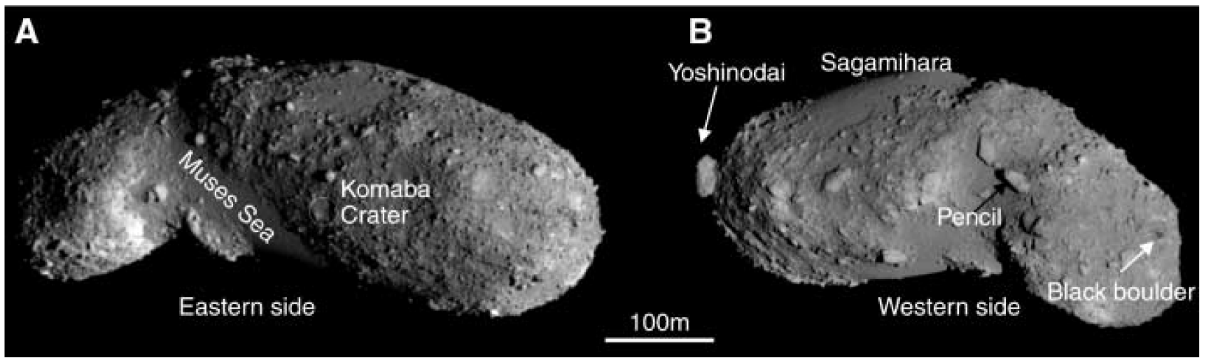
Figure 1: Global images of near-Earth asteroid Itokawa recorded from the Hayabusa spacecraft. Note the scale! (Figure from Saito2006)

Since 1991, when the Galileo spacecraft flew by the asteroid (951) Gaspra, asteroids have been targeted by spacecraft several times, see table 1 (see also Farquhar2002, for a slightly outdated review).

Spectacular insights were gained from results of the asteroid rendezvous missions NEAR-Shoemaker and Hayabusa. NEAR-Shoemaker orbited the near-Earth asteroid (433) Eros for about a year until it successfully soft-landed in February 2001, taking further data from ground. Hayabusa hovered within kilometers from the small (effective diameter around $320\text{\,}\mathrm{m}$) near-Earth asteroid (25143) Itokawa for several months in 2005—note that stable spacecraft orbits around such a low-gravity target are hard to find. After intensively studying the asteroid (see, e.g., Fig. 1), Hayabusa touched down on the surface twice to take samples of surface material. Unfortunately, the spacecraft is experiencing technical difficulties and it is unclear whether samples have been taken. Hayabusa is scheduled to return the sample container to Earth in 2010. First Hayabusa results were published in a special issue of Science on 2 June 2006 (Vol. 312, issue 5778).

Asteroid missions are currently being planned at all major space agencies:

Dawn

is a NASA mission to rendezvous with the two large main-belt objects (1) Ceres and (4) Vesta, scheduled for launch in June 2007, arrival at Vesta in 2011 and at Ceres in 2015. Italian and German institutes (including DLR Berlin) contribute two science instruments (Russel2006).

Don Quijote

is an ESA mission to produce a measurable deflection of a near-Earth asteroid. The mission will consist of two spacecraft, a kinetic impactor and an orbiter which will intensively study the asteroid before and after the deflecting impact. Don Quijote is currently under phase-A study (HarrisDQ).

Hayabusa 2

is basically a clone of Hayabusa by the Japan Aerospace Exploration Agency JAXA. Hayabusa 2 is planned to be launched in 2010 or 2011 and to return samples from another near-Earth asteroid. An improved version, named Hayabusa Mark 2, is also being planned (Yoshikawa2006).

OSIRIS

is a sample-return mission to a near-Earth asteroid currently under consideration at NASA. If selected for further development, the mission may be launched in 2011.

Spacecraft studies of asteroids benefit significantly from ground-based studies of their targets, and vice-versa. Mission planning, in particular, is severely hampered by the general lack of information on the physical properties of potential targets. Physical studies of potential spacecraft target asteroids are of crucial importance in this respect.

2 Asteroid populations and their origins

Since 1 Jan 1801, when Piazzi discovered (1) Ceres, the number of known asteroids has increased dramatically. As of 2 May 2007, 374,256 asteroids are known, 157,788 of them have well-established orbits (see http://cfa-www.harvard.edu/iau/lists/ArchiveStatistics.html). Both numbers are increasing by the thousands per month due mostly to dedicated asteroid discovery programs. New telescope systems, which are currently being built (such as Pan-STARRS, see PanSTARRS), are expected to result in a further increase of the asteroid discovery rate.

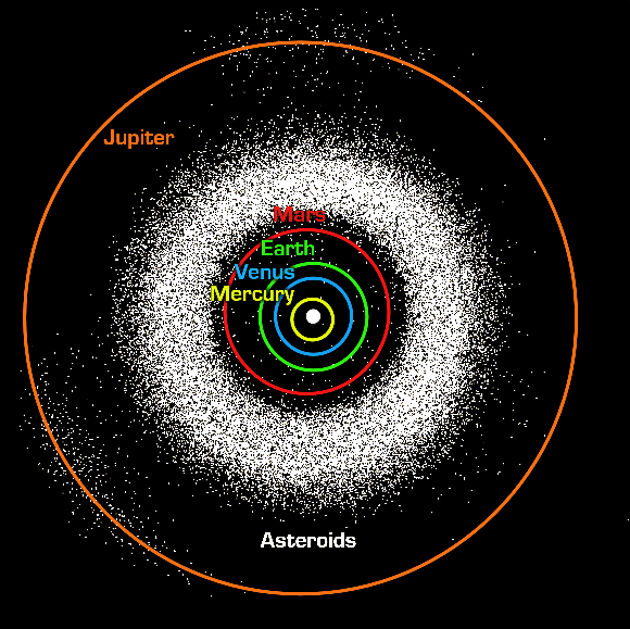
Figure 2: Asteroids in the inner Solar System out to Jupiter. Note the presence of some asteroids close to the terrestrial planets. Figure credit: NASA/JPL-Caltech/R. Hurt (SSC-Caltech).

As can be seen from Fig. 2, there are three main asteroid populations in the inner Solar System:

Main-belt asteroids (MBAs)

Most known asteroids orbit the Sun in the region between the orbits of Mars and Jupiter, called the asteroid belt or main belt. The accretion process in the main belt stopped before a planet could be formed, probably due to dynamical excitation through the gravity of forming Jupiter; present MBA encounter velocities are so high that collisions are more likely to produce fragmentation than accretion (Petit2002). MBAs are thus remnant planet building material, left-overs from the formation of the Solar System which have undergone only limited processing in the past .

The largest main-belt object is (1) Ceres with a diameter around $950\text{\,}\mathrm{km}$. The observed asteroid size-frequency distribution increases steeply with decreasing size, but drops towards small sizes due to observational incompleteness (in other words: the smallest asteroids have not been discovered, yet). The smallest newly-discovered MBAs are typically a few k m  in diameter.

Near-Earth asteroids (NEAs)

Since the discovery of (433) Eros in 1898 it is known that there is an intriguing population of asteroids which approach Earth. The Earth-like orbits of some NEAs make them accessible for spacecraft with only a moderate amount of propellant and thus at a relatively low cost.

On average, NEAs are significantly smaller than the known MBAs; the largest NEA is (1036) Ganymede with an estimated diameter around $32\text{\,}\mathrm{km}$, objects as small as a few tens of meters have been detected. As of 1 May 2007, 4619 NEAs have been discovered, including 712 objects with an estimated diameter of $1\text{\,}\mathrm{km}$ or larger. The total number of the latter is estimated to lie between 700 and 1,100 (Werner2002; Stuart2004).

A particularly noteworthy group of NEAs are the Potentially Hazardous Asteroids (PHAs), which approach Earth’s orbit to within and have diameters above $150\text{\,}\mathrm{m}$. As of 7 May 2007, 860 PHAs are known.

Jupiter Trojans

There are two large asteroid groups beyond the main belt, collectively referred to as Jupiter Trojans. They are in stable 1:1 resonance with Jupiter, librating around the $L_{4}$ and $L_{5}$ Lagrange points which lead and trail the planet by $60\text{\,}\mathrm{\SIUnitSymbolDegree}$ in heliocentric ecliptic longitude, respectively.

The origin of the Trojans is currently under debate. While they were long believed to have formed near their present position (see, e.g., Marzari2002), it has been argued by Morbidelli2005 that their orbital distribution indicates they were captured by Jupiter during the time of the Late Heavy Bombardment, and that they share a volatile-rich parent population with comets and small bodies in the outer Solar System. The latter theory is supported by the rather uniform spectral properties and albedos of Trojans similar to cometary nuclei (Barucci2002) and with recent physical studies of large Trojans (Marchis2006; Emery2006).

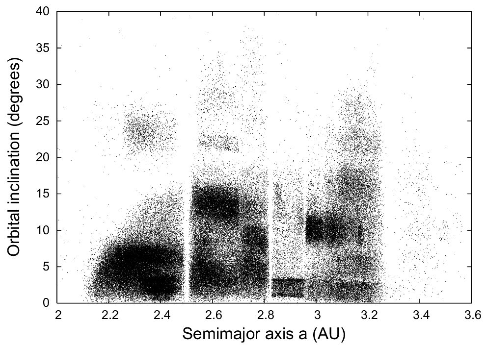
Figure 3: Scatter plot of the orbital parameters of numbered MBAs. The Kirkwood gaps are clearly seen, e.g. at semimajor axes of $a\sim$2.5\text{\,}\text{AU}$$ (3:1 mean-motion resonance with Jupiter), at some (5:2 resonance), roughly (7:3 resonance), and the sharp boundary shortward of (2:1 resonance). Also some significant clusters corresponding to asteroid families are clearly seen, e.g. the Koronis family situated at low inclinations between the 5:2 and 7:3 resonances, seen as a relatively sharp rectangle. (Orbital parameters were retrieved from the University of Pisa AstDys service, http://hamilton.dm.unipi.it, on 8 Jan 2007)

Orbits inside the main belt are highly chaotic, mostly due to the gravitational influence of massive and near-by Jupiter. In particular, many main-belt orbits are unstable due to resonance with Jupiter; there is a significant depletion in objects on such orbits, the Kirkwood gaps (Kirkwood1869, see also Fig. 3).

Asteroid families

While the largest MBAs are believed to be primordial, most MBAs below a certain threshold size appear to be fragments of larger parent bodies which underwent a catastrophic collisional disruption (Nesvorny2006). One might expect fragments of such a breakup event to be on rather similar orbits. Indeed, as can be seen in Fig. 3, there are statistically significant clusters in the orbital elements of MBAs referred to as asteroid families, which were first noticed and explained by Hirayama (see Zappala2002, for a review). The reflection spectra of asteroids belonging to a family are generally very similar, confirming their common origin (Cellino2002).

Most known asteroid families appear to be very old, on the order of several (Carruba2003). Due to chaotic dynamics, asteroid families disperse over timescales of roughly , making old families hard to detect dynamically (Nesvorny2002b). The ages of very young families, on the other hand, can be determined directly, by numerically integrating the orbits of family members backward in time until convergence is reached; a spectacular case is that of the Karin cluster, the age of which has been determined by Nesvorny2002 to be only . The convergence of this backward integration has been shown to improve significantly if the Yarkovsky effect (see sect. 3) is taken into consideration (Nesvorny2004). Recently, asteroid families even younger than have been reported by NesvornyVokrouhlicky2006.

The origin of NEAs

It is now widely accepted that the dominant NEA source population is the main belt, followed by extinct cometary nuclei providing of the population (see BinzelLupishko2006, and references therein). This is consistent with the diversity in spectral properties and albedo observed among NEAs, which is similar to that of MBAs.

The only known means of delivering sufficient numbers of MBAs into near-Earth space is through resonances with Jupiter and later perturbations by the inner planets, which may temporarily trap them in near-Earth orbits, although collisions with the Sun or ejection out of the Solar System are more likely (see, e.g., Morbidelli2002, and references therein).

The timescale for resonant ejection out of the main belt is a few M yr, the dynamical lifetime of NEAs is on the order of . However, as apparent from the crater record on terrestrial planets and their satellites, the NEA population has been rather stable over the past (Ivanov2002; Werner2002). This suggests a steady effect which continuously replenishes the NEA source regions.

It is now widely believed that this is accomplished by the Yarkovsky effect (see sect. 3). The Yarkovsky-induced drift inside the main belt takes much longer than the actual resonance-driven transport into near-Earth space, it is therefore the strength of the Yarkovsky effect that determines the timescale and size-dependent efficiency of NEA delivery (Morbidelli2003). This is supported by the observed cosmic-ray exposure ages of meteorites, which average around for stony meteorites and an order of magnitude larger for iron meteorites, significantly longer than the NEA dynamical lifetime and indicative of a substantial drift time spent inside the main belt (see, e.g., Bottke2006, and references therein).

3 The Yarkovsky and YORP effects

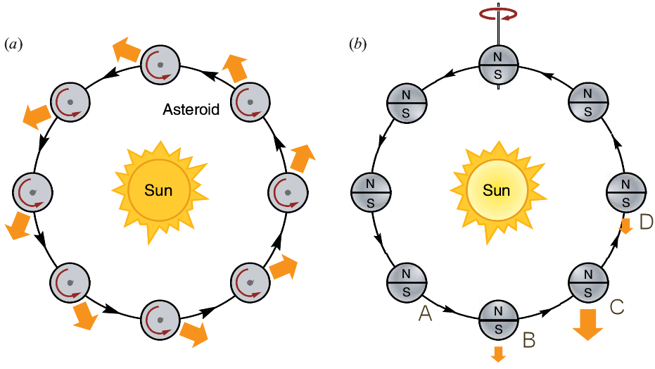
Figure 4: (a): Schematic depiction of the diurnal Yarkovsky effect for a spin axis perpendicular to the orbital plane. Due to thermal inertia, the trailing afternoon side of a prograde rotator is hotter than the leading morning hemisphere, leading to an emission surplus from the former. The resulting net force (arrows) has an accelerating component tangential to the orbit, causing most prominently a secular increase in orbital semimajor axis $a$ (the radial force component is typically negligible against solar gravity). Analogously, retrograde rotators are decelerated by the Yarkovsky effect, their $a$ decreases. (b): Seasonal Yarkovsky effect, with the spin axis inside the orbital plane. There is an emission surplus from the summer hemisphere. Thermal inertia causes a phase shift between seasons and orbital revolution (orange arrows), leading to a net tangential force component after averaging over one orbit (see positions A–D). The seasonal effect always decreases $a$. (Figure adapted from Bottke2006).

It has been realized over the past decade that asteroid dynamics is governed not only by gravity and mutual collisions, but also by the non-gravitational Yarkovsky and YORP effects, both caused by the recoil force from thermally emitted photons. As with ion spacecraft propulsion, the resulting momentum transfer is slight but steady, and therefore capable of slowly but substantially altering the orbits (Yarkovsky effect) and spin states (YORP effect) of small asteroids or meteoroids. Both effects have been observed (see below). See Bottke2006 for a recent review.

Yarkovsky effect

As depicted in Fig. 4, surface temperature asymmetries due to thermal inertia (see sect. 8) lead to a gradual increase or decrease in orbital semimajor axis $a$, depending on the spin axis orientation and obliquity. There are diurnal and seasonal components of the Yarkovsky effect, which are respectively most efficient in the situations depicted in Fig. 4.

Since the Yarkovsky effect is driven by surface temperature asymmetries, it depends crucially on the thermal inertia. Specifically, it vanishes in the limiting cases of zero and infinite thermal inertia where the temperature distribution is symmetric about the subsolar point. Obviously, spin rate and heliocentric distance are also relevant.

Very importantly, the Yarkovsky effect is size dependent: For objects much larger than the penetration depth of the heat wave (typically at the c m -scale) and all other parameters kept constant, the photon recoil force scales with $D^{2}$ (with diameter $D$), while the mass scales with $D^{3}$, so the acceleration scales with $D^{-1}$. Smaller objects become increasingly isothermal, weakening the Yarkovsky effect; their interaction with the solar radiation field is dominated by the Poynting-Robertson effect or the radiation pressure.

There is now ample evidence that the Yarkovsky effect strongly influences the orbital dynamics of asteroids below in diameter:

• The small NEA (6489) Golevka was shown by YarkoGolevka to have undergone an orbital drift in the years 1991–2003 which cannot be explained by gravitational perturbations alone, but is fully consistent with an additional Yarkovsky-induced drift. The Yarkovsky effect had previously been found to alter the orbit of the LAGEOS satellite (Rubincam1987; Rubincam1988; Rubincam1990).

• As seen above, there must be a steady mechanism bringing small MBAs into powerful resonances which deliver them into near-Earth space—only the Yarkovsky effect is known to do so in a way consistent with the observed NEA distributions in size, spectral type, and spin axis obliquity. In particular, its size dependence explains the apparently different size-frequency distributions of NEAs and MBAs (see Delbo2007, for a detailed discussion).

• The Yarkovsky effect is required to explain the observed orbital distribution inside asteroid families. Most spectacularly, the orbits of asteroids belonging to the very young Karin family (see above) were seen to have evolved under the Yarkovsky effect (Nesvorny2004). Furthermore, Yarkovsky-induced drift is required to make the observed orbital dispersion in evolved asteroid families compatible with that of young families and also with model calculations of the initial fragment ejection velocity distribution (Carruba2003; Bottke2006).

• The Yarkovsky effect is crucial to assess the impact hazard from individual asteroids. Specifically, it determines whether the NEA 1950 DA, the object with the highest currently known impact probability (see sect. 4), will hit Earth in 2880 or not (Giorgini2002).

YORP effect

The photon recoil force combined with the radiation pressure of absorbed sunlight may also cause a net torque, altering the spin axis obliquity and the rotation rate of small objects. The YORP torque depends critically on the object’s shape, in particular it vanishes for spherical or ellipsoidal objects (see Scheeres2007, for a recent definition of a shape-dependent parameter describing the strength of the YORP torque). While small asteroids are known to have highly irregular shapes in general, the shape of individual objects is usually unknown, although that situation is likely to improve significantly in the next decade (see sect. 4). The YORP effect is therefore less well studied than the Yarkovsky effect.

Nevertheless, the first direct observations of YORP-induced shifts in rotational period have very recently been reported for the NEAs (1862) Apollo (Kaasalainen2007) and (54509) YORP (Lowry2007; Taylor2007, 54509 was known as 2000 PH5 before 2 April 2007; see also sect. 4). The YORP effect was seen by Vokrouhlicky2003 to determine the distribution of spin axis obliquities in asteroid families. The YORP effect may also explain the observed size-dependence of asteroid spin-rate distributions (see sect. 3) and may be important in the forming of binary asteroid systems (see sect. 6).

4 Asteroids impacting Earth: Hazard and link to meteorites

The terrestrial planets and their satellites have been resurfaced by impact cratering. This is quite evident on bodies such as the Moon or Mars, where erosion processes are relatively slow, but also on Earth a significant number of impact craters has been preserved—the most widely known in Germany is the Nördlinger Ries.

Most Earth impactors are very small in size and are completely destroyed upon atmospheric entry causing only a “falling star”. Among objects that reach the ground, the majority is barely large and robust enough to do so—these produce meteorites which represent the major source of extraterrestrial material available for study in Earth laboratories. Large impactors some thousand tons in mass or above, however, are not significantly decelerated by the atmosphere. They hit the ground at velocities above the Earth escape velocity of $11.2\text{\,}\mathrm{km}\text{\,}{\mathrm{s}}^{-1}$ and release their correspondingly large kinetic energy in a crater forming process. While our understanding of the latter is still highly incomplete (see, e.g., Holsapple2002; deNiem2005, and references therein) it is clear that impactors with diameters around $1\text{\,}\mathrm{km}$ release a significantly higher amount of energy than a nuclear warhead; such impacts would cause global catastrophes (see, e.g., Morrison2002; Chapman2004b, for reviews). The Cretaceous-Tertiary extinction event, during which the dinosaurs died out, is widely believed to have been caused by the impact of an object around $10\text{\,}\mathrm{km}$ in diameter (Alvarez1980).

The US Congress held hearings to investigate the impact hazard and charged NASA with the task of discovering $90\text{\,}\%$ of all near-Earth objects (NEOs) larger than $1\text{\,}\mathrm{km}$ in diameter within ten years; this Spaceguard Survey was initiated in 1998, the due date for the spaceguard goal is end of 2008. Several successful asteroid discovery programs have been initiated leading to a steep and ongoing increase in asteroid discoveries. A follow-up discovery program, possibly requiring NASA to discover $90\text{\,}\%$ of all NEOs above $140\text{\,}\mathrm{m}$ in diameter until 2020, is currently under discussion. It might include the deployment of mid-infrared space telescopes for asteroid discovery, such as the proposed NASA mission NEOCam (Mainzer2006).

As of 7 May 2007, the highest known Earth impact probability for an individual object is $0.33\text{\,}\%$ for a potential impact of the $1.1\text{\,}\mathrm{km}$ wide NEA (29075) 1950 DA in 2880 (Giorgini2002)—the only known impact probability larger than the accumulated background risk due to unknown objects of comparable size, thus leading to a positive hazard rating on the Palermo scale by PalermoScale. It is worth pointing out that the uncertainty in the risk assessment by Giorgini2002 is dominated by the lack of knowledge of physical properties of the asteroid which govern the magnitude of the Yarkovsky effect.

The NEA (99942) Apophis (then known as 2004 MN4, in diameter, see Delbo2007b) held, for a brief period after its rediscovery in December 2004, an unprecedentedly large probability for an impact in 2029, peaking at $2.7\text{\,}\%$ and severely disconcerting the NEA community over the Christmas holidays. On 27 Dec 2004 the 2029 impact could be ruled out on the basis of newly obtained astrometric data; the miss distance from the geocenter in 2029 is currently estimated to be $5.89\pm 0.35$ Earth radii ($3\sigma$ uncertainty; Chesley2006). The subsequent orbit, however, will be severely perturbed by Earth’s gravity, possibly onto impact course. The corresponding risk is dominated by a potential impact in 2036, with a probability of $2.2\cdot 10^{-5}$. Again, for accurate risk assessment the Yarkovsky effect must be taken into consideration (Chesley2006).

The design of asteroid deflection missions, which would become necessary if an impactor were to be discovered, is an active area of engineering research (see, e.g., Kahle2006). ESA is planning a precursor mission to an asteroid deflection mission, Don Quijote, which is currently under phase-A study (see sect. 1).

5 Physical properties of asteroids

There is a growing body of information on the physical properties of asteroids, although the rapid discovery rate leaves most known objects uncharacterized. Some asteroids, however, have been scrutinized with spacecraft or have been studied by ground-based observers in great detail.

The emerging picture is still rather incomplete and highly diverse.

1 Diameter and albedo

For most asteroids, the size, arguably the most basic physical property, is only poorly known. Note that asteroids are typically far too small to be spatially resolved with current telescopes. In only a few cases could asteroid sizes be determined by means of direct imaging from near-by spacecraft, the Hubble Space Telescope, or ground-based telescopes equipped with adaptive optics. Another rather direct way of determining asteroid sizes is from observations of stellar occultations.

For most asteroids, only optical photometric data are available, typically from astrometric measurements with limited photometric accuracy. The amount of reflected sunlight is proportional to the projected area and the albedo, allowing coarse conclusions on the size to be drawn. An important quantity is the absolute optical magnitude $H$, which is defined as the visual magnitude corrected to heliocentric and observer-centric distances of and a solar phase angle of $0\text{\,}\mathrm{\SIUnitSymbolDegree}$ (HG). $H$ is related to diameter $D$ and geometric albedo $p_{\text{V}}{}$ by (FowlerChillemi):

$$D=10^{-H/5}\frac{$1329\text{\,}\mathrm{km}$}{\sqrt{p_{\text{V}}{}}}.$$ (1)

Asteroid albedos range from some $p_{\text{V}}{}=0.02$ up to around 0.6, thus diameters estimated in this way are very uncertain.

A widely used method to determine asteroid sizes is from observations of their thermal emission, which is proportional to the projected area but only a weak function of albedo (see chapter 2 for a detailed discussion). This method, pioneered by Allen1970, is the source of most known asteroid diameters (SIMPS). Other methods of determining asteroid sizes include observations at radar wavelengths (Ostro2002).

Alternatively, the diameter can be determined if $p_{\text{V}}{}$ is known. Methods for determining asteroid albedos include studies of the optical brightness and also of the polarization of reflected sunlight as a function of solar phase angle (see Muinonen2002, for a review; note that the latter method is so far based on a purely empirical correlation between albedo and certain polarization properties).

2 Taxonomy

Conclusions on the mineralogical composition of asteroid surfaces can be drawn from reflection properties at visible and near-IR wavelengths, chiefly from spectral features and albedo measurements. Asteroid reflection properties are routinely compared to those of meteorites. This way, much could be learned about the composition of asteroids and about the origin of most meteorites.

Different kinds of taxonomic systems are used in order to describe observed asteroid reflection properties, and also to link them with analogue meteorites. The most widely used taxonomic systems are those by Tholen1984 and BusBinzel. While taxonomic classification relies chiefly on spectroscopic or spectrophotometric observations, it can be greatly constrained with albedo measurements alone.

A large number of taxonomic classes have been proposed, but most asteroids belong to one of the following classes (or “complexes” in the notation of BusBinzel) with generally mnemonic names:

C

is for carbonaceous: C-type asteroids display spectra and albedos consistent with a composition similar to that of carbonaceous chondritic meteorites. They are very dark, generally $p_{\text{V}}{}<0.1$. Most objects in the outer main belt appear to be C types (see BusBinzel, Fig. 19).

S

is for silicaceous: S-type asteroids show spectral features indicative of a silicate composition similar to stony meteorites, with $p_{\text{V}}{}$ normally in the range from 0.10 to 0.25.

S types dominate the inner main belt and the near-Earth population. S-type asteroids are therefore commonly associated with the most frequent meteorite type, the ordinary chondrites. However, the spectral features and albedos of the similar but less frequent Q-type asteroids fit those of ordinary chondrites much better. It is widely believed that S and Q-type asteroids are of identical bulk mineralogy, and that their surfaces age due to impacts by micro-meteorites and/or the solar wind (note that meteorites have lost their original surface during atmospheric entry), this process is called space weathering. In this picture, S and Q-type asteroids are respectively the old and young endmembers of a continuum; spacecraft imaging of the S-type asteroids Ida and Eros appears to support this idea (see Clark2002; Chapman2004, for reviews). Recently, Lazzarin2006 found evidence that asteroids of other spectral types are also space weathered.

X or EMP

Most remaining asteroids have rather featureless spectra at visible wavelengths, they are called X-type asteroids. There are three distinct groupings of X types differing in albedo:

E

with high albedo ($p_{\text{V}}{}>0.3$), probably related to enstatite achondrite meteorites

M

with moderate albedo ($0.1<p_{\text{V}}{}<0.2$), some of which appear to be related to iron meteorites, but others appear to be non-metallic

P

with very low albedo ($p_{\text{V}}{}<0.1$). P-type asteroids are believed to be composed of silicates very high in organic material, there are no known meteorite analogues. Together with the equally dark D-type asteroids (not listed here), P types are very abundant among the Jupiter Trojans. Some D and P-type asteroids in the near-Earth population are believed to be extinct cometary nuclei (depending on their orbital properties).

For X types, an albedo determination is particularly diagnostic of mineralogical composition. The study of composition and possible subtle spectral features of X-type asteroids is a very active area of research.

3 Spin rate

Asteroid spin rates differ significantly from object to object, from only a few minutes up to several weeks. The rotation states of MBAs are mostly determined from mutual collisions: The observed spin rates of MBAs larger than $50\text{\,}\mathrm{km}$ in diameter follow a Maxwellian distribution as predicted by this model, with a mean rotation period around $10\text{\,}\mathrm{h}$ (HarrisPravecACM2005). Smaller asteroids deviate, increasingly so with decreasing size, from a Maxwellian distribution. In comparison, both very low and very high rotation rates are over-represented, indicating the presence of an effect capable of spinning small asteroids up or down. The YORP effect is widely believed to be responsible for this (HarrisPravecACM2005).

There is an intriguing dichotomy in asteroid spin rates: While the periods of all known asteroid larger than $1\text{\,}\mathrm{km}$ in diameter are larger than $2.2\text{\,}\mathrm{h}$, most smaller objects spin significantly faster, at spin rates of only a few minutes in extreme cases. This is widely seen as indicative of their internal structure (see sect. 5).

4 Shape and spin axis

The shape and spin axis of most asteroids are unknown. It must be kept in mind that asteroids are typically too small to be spatially resolved. There are two well-established techniques to determine physical models of asteroid shape and spin state from ground-based observations, namely from time-resolved photometric observations at optical wavelengths (see Kaasalainen2002) or from radar observations of their rotationally induced Doppler frequency shift (Ostro2002). Both methods typically require a large amount of input data taken at various aspect angles. Note that shape models obtained from the inversion of optical photometry are typically convex, concavities are virtually impossible to resolve using that technique.

Asteroid shapes found so far vary significantly: Larger MBAs are typically nearly spherical, although there are notable exceptions such as the “dog-bone shaped” asteroid (216) Kleopatra (Kleopatra). The shape diversity of smaller asteroids, most of which are expected to be collisional shards, is significantly larger. Upcoming asteroid discovery programs such as Pan-STARRS promise to provide an extensive database of well-calibrated optical photometric data, which will allow the shapes and spin states of at least several thousands of asteroids to be determined in the next decade (Durech2005).

5 Internal structure—are asteroids piles of rubble?

The internal structure of asteroids is an important and very active area of research. In particular it is not clear whether asteroids have significant tensile strength or whether some (or most) are loose gravitational aggregates, called rubble piles (see Richardson2002, for a review). This is of particularly practical importance in the case of potential Earth impactors: Rubble piles may be significantly harder to deflect than monolithic objects.

Surface morphology

The two asteroid rendezvous missions carried out so far revealed that Eros does not appear to be a rubble pile (Cheng2004) while Itokawa does (Fujiwara2006). Flyby imaging revealed very large craters, comparable to the objects’ radii, on some asteroids (Gaspra, Ida, and Mathilde) and on Mars’ satellite Phobos, presumably a captured asteroid. Those large craters are largely seen as indicative of a very weak, rubble-pile-like internal structure (see, e.g., Chapman2002; Cheng2004, and references therein) because monolithic bodies would be expected to be disrupted by shock waves such as those generated during the crater-forming impacts. Weak, porous bodies dissipate shock waves efficiently and can therefore sustain much larger impacts (Holsapple2002). This is supported by the presence of adjacent and undisturbed large craters on Mathilde; on a solid target, the formation of the later crater would have significantly affected the former.

Mass density

Inferences on internal structure can be made from the mass density, which is known for a small set of asteroids consisting of spacecraft targets, some binary systems (see sect. 6), and a few asteroids which made recent close encounters with other asteroids (Hilton2002). While the bulk mass densities of the largest MBAs above $500\text{\,}\mathrm{km}$ in diameter match those of analogue meteorites very well, smaller objects are significantly under-dense. There is a cluster of objects, including Eros, with macroporosities around $20\text{\,}\%$ (i.e. $20\text{\,}\%$ of the volume is apparently void) which are believed to contain major cracks formed by shattering through sub-catastrophic impacts. Other objects display much higher macroporosities, beyond $50\text{\,}\%$ in extreme cases; these objects must contain major voids and are widely believed to be rubble piles (Mathilde falls into this category, which is consistent with its craters mentioned above) (see Britt2002, for a review).

It is worth noting that the uncertainty in mass density is typically dominated by the diameter uncertainty (see Merline2002; Richardson2006).

Spin rate

Further information can be potentially obtained from the observed dichotomy in asteroid spin rates (see sect. 3): As was first noted by Harris1996, the apparent “spin barrier” around $2.2\text{\,}\mathrm{h}$ coincides with the spin rate at which the centrifugal force at the equator of a spherical body equals gravity. Rubble piles at faster spin rates would therefore disrupt, the conspicuous lack of such fast rotators larger than $1\text{\,}\mathrm{km}$ appears to indicate that most, if not all, of them are rubble piles. Small fast rotators, on the other hand, are held together by tensile strength and are expected to be monolithic.

Both conclusions have recently been challenged by Holsapple2007 who argues that for bodies larger than some $10\text{\,}\mathrm{km}$ in diameter, tensile strength is negligible relative to gravity.As a result, such asteroids are subject to the quoted spin barrier even if they possess significant tensile strength. Holsapple2007 estimated the tensile strength required to stabilize known small fast rotators to be on the order of only $10--100\text{\,}\mathrm{kPa}$, “the strength of moist sand” in the words of the author.

6 Binarity

An intriguing asteroid sub-population is that of the binary asteroids, i.e. asteroids with a gravitationally bound satellite. The first asteroid satellite, Dactyl, was found orbiting the MBA (243) Ida through imaging from the Galileo spacecraft (Belton1996). Since then, some 70 binary asteroid systems have been discovered, using different observational techniques. Their orbits range from near-Earth space out into the trans-Neptunian region, with primary body diameters between just a few kilometer and several hundred (Richardson2006; Noll2006).

The mass, which for asteroids is only rarely known (see Hilton2002), can be calculated for binary systems from Newton’s form of Kepler’s Third Law if the mutual orbit is well constrained.

The total angular momentum of most small NEA binaries is just above the critical limit at which a single body of equal mass would disrupt. This indicates that they were formed from a parent body which was spun up (e.g. through the YORP effect), ultimately leading to its fission into a binary system (HarrisPravecACM2005). This is seen as an indication for their being rubble piles (see sect. 5), which is consistent with the low lightcurve amplitude of most binaries.

7 Regolith

Large atmosphereless bodies such as Mars, Mercury, or our Moon are known to be covered with a thick layer of regolith, which formed from retained impact ejecta. Large asteroids are known to display at least some regolith on their surfaces, smaller objects are known to be increasingly depleted in fine dust grains (see, e.g., Dollfus1989). This latter finding was explained with the low asteroid gravity which allows fine impact ejecta (with higher average thermal velocities) to escape. Asteroids below a certain threshold size were thus expected to be basically regolith free, the threshold diameter was estimated to be between 10 and $70\text{\,}\mathrm{km}$ (see Scheeres2002, for a review). This was consistent with the findings of Lebofsky1979 and Veeder1989, who indirectly estimated the thermal inertia (see sect. 8) of a number of small NEAs to be very high, indicating a lack of thermally insulating regolith on their surfaces.

To the big surprise of the asteroid community, however, spacecraft imaging in 1991 (see sect. 1) revealed indications for a substantial regolith layer on the MBA (951) Gaspra with an effective diameter of only $12\text{\,}\mathrm{km}$. The NEA (433) Eros, around $17\text{\,}\mathrm{km}$ in diameter, was unambiguously seen to be thickly covered with regolith, although an intriguingly large number of boulders are present on its surface. Even the small NEA (25143) Itokawa (effective diameter around $320\text{\,}\mathrm{m}$) is not entirely regolith free: recent spacecraft imaging showed a thought-provoking surface dichotomy between boulder-strewn surface patches, apparently devoid of powdered material, and very flat, regolith-dominated regions (see Fig. 1 on p. 1).

While the origin of regolith on asteroids is far from being completely understood, it is plausible that the regolith found on relatively small asteroids indicates a weak surface structure, i.e. low material strength and/or high porosity (see, e.g., Asphaug2002; Chapman2002; Holsapple2002; Scheeres2002). In this case, crater formation is dominated by gravity rather than material strength, which reduces ejecta velocities and enables the gravitational retention of a non-negligible fraction thereof. This conforms with first results from the Deep Impact mission (AHearn2005), where a $370\text{\,}\mathrm{kg}$ projectile hit the nucleus of comet 9P/Tempel 1 at a relative velocity of $10.3\text{\,}\mathrm{km}\text{\,}{\mathrm{s}}^{-1}$—apparently a significant fraction of the ejected dust was very slow and later reaccumulated, indicative of a very low material strength of the nucleus. We caution, however, that the formation and later dynamics of ejecta is likely to be very different among comets and asteroids.

No detailed spacecraft imaging is available for asteroids between $0.32\text{\,}\mathrm{km}$ (Itokawa) and $12\text{\,}\mathrm{km}$ (Gaspra) in diameter; it is therefore unclear if they display regolith or not. In particular it is unclear whether there is a clear transition size above which asteroids are fully covered with regolith, while smaller objects are not. In the light of the previous paragraph, studies of asteroid regolith coverage may allow conclusions to be drawn on the elusive but important material strength and may further our understanding of regolith formation through impact processes.

8 Thermal inertia

Thermal inertia is a measure of the resistance to changes in surface temperature: The surface of a body with low thermal inertia heats up or cools down readily, while bodies with high thermal inertia tend to keep their surface temperature for longer (see sect. 2 for a more detailed discussion).

Thermal inertia governs the important Yarkovsky and YORP effects (see sect. 3); thermal inertia estimates are crucial for model calculations of both. Thermal inertia also determines the temperature environment in which lander missions (see, e.g., Binzel2003, for some considerations) have to operate: Low thermal inertia causes harsh temperature contrasts between the day and the night side, while in the case of high thermal inertia the diurnal temperature profile is much smoother. Furthermore, thermal inertia is a very sensitive indicator for the presence or absence of regolith on the surface (see sect. 7): The thermal inertia of lunar regolith is some 50 times lower than that of bare rock, which in turn is nearly an order of magnitude below that of metal (see table 1 on p. 1). This is widely used in planetary science; several Mars orbiters, e.g., carried temperature sensitive instruments in order to derive global thermal-inertia maps by means of which exposed bedrock can be distinguished from regolith (see, e.g., Christensen2003; Putzig2005, and references therein).

Little is known so far about the thermal inertia of asteroids, virtually nothing is known about the thermal inertia of small asteroids including NEAs. Ground-based determinations of asteroid thermal inertia are challenging, both in terms of observing and modeling: Extensive spectrophotometric or spectroscopic observations in the difficult mid-infrared wavelength range ($\sim 5$–$35\text{\,}\mathrm{\SIUnitSymbolMicro m}$) are needed (see sect. 3). Such observations are hampered by the large atmospheric opacity throughout most of this wavelength range, combined with a large level of background radiation stemming from the atmosphere, clouds, and the telescope itself which emits thermal radiation peaking at a wavelength around $10\text{\,}\mathrm{\SIUnitSymbolMicro m}$. On the modeling side, difficulties arise because crucial parameters such as the object’s shape and spin state are typically not known. Furthermore, sufficiently detailed thermophysical models had so far only been tested for application to large MBAs, which differ from small NEAs in many important ways (see HarrisLagerros2002, for a review and chapter 3 for a detailed discussion).

It was realized already in the 1970s that the typical thermal inertia of large asteroids must be small, comparable to that of the Moon (see, e.g., Morrison1977, for a review). However, no quantitative results were available, with the notable exception of (433) Eros (LebofskyRieke1979, based on a very approximate shape model) and (1) Ceres and (2) Pallas (Spencer1989). The first large-scale thermal-inertia study was by MuellerLagerros1998 who quantitatively determined the thermal inertia of 5 large MBAs.

There has been some controversy about the typical thermal inertia of NEAs, which had not been measured directly so far. LebofskyBetulia; Lebofsky1979 and Veeder1989 found indirect evidence that a significant fraction of NEAs should have a very high thermal inertia indicative of a surface consisting of bare rock. Delbo2003, on the other hand, performed a thermal spectrophotometric survey of NEAs and stated that the majority of their targets must possess a thermally insulating layer of regolith. Note that the thermal inertia of small asteroids is particularly relevant since they are substantially influenced by the Yarkovsky effect (see sect. 3) which is governed by thermal inertia.

6 Scope of this work

The primary aim of this work is to augment the number of asteroids with known thermal inertia. Emphasis is put on NEAs for which practically no reliable information is available so far. We have also determined the size and albedo of two asteroid targets of upcoming spacecraft visits.

The following questions are addressed:

• What is the typical thermal inertia of NEAs?

• What can be learned about their regolith coverage?

• Does thermal inertia depend on size, as might be expected from models of regolith retention?

• What is the size and albedo of our targets, and how can we constrain their surface mineralogy?

This requires extensive observations of the thermal emission of our targets in the mid-infrared wavelength range ($\sim 5$–$35\text{\,}\mathrm{\SIUnitSymbolMicro m}$), combined with observations of the reflected sunlight and a suitable model of the thermal emission.

An adequate thermophysical model for NEAs has been developed and tested (see chapter 3). Previously available models of NEA thermal emission are not sufficiently detailed for the quantitative determination of thermal inertia, while available thermophysical models for atmosphereless bodies (on which the model described herein is based) were neither designed nor tested for application to NEAs.

Observations were made with the NASA Infrared Telescope Facility on Mauna Kea / Hawai’i (chapter 4) and the Spitzer Space Telescope (chapter 5).

We present detailed studies of individual objects rather than a general survey; our results for individual asteroids are presented in chapter 6. Nevertheless, our results allow the first firm conclusions to be drawn on the NEA distribution in thermal inertia. These and other results are discussed in chapter LABEL:chapt:discussion.

In the final chapter LABEL:chapt:conclusions our main conclusions are summarized, possible future work is discussed in chapter LABEL:chapt:future.

Chapter 2 Thermal emission of asteroids

In this chapter we briefly summarize some goals and methods of the study of asteroid thermal emission. After a brief overview section (sect. 1), those physical properties which are most relevant for the thermal emission of asteroids will be introduced in sect. 2 (a more detailed discussion of some will be given in chapter 3). The observing conditions in the mid-infrared wavelength-range, in which the thermal emission of asteroids typically peaks, will be discussed in sect. 3.

There are two different ways of interpreting thermal data, depending on the available database and other previous knowledge about the particular asteroid. If only little information is available, the diameter and albedo can be estimated, but assumptions must be made about thermal properties such as thermal inertia. If, however, much information is available, thermal properties can be derived from the thermal data, in addition to potentially more accurate estimates of diameter and albedo.

Two “simple” thermal models which are widely used to determine asteroid diameters and albedos are presented in sect. 4. Throughout this work, we make frequent use of the Near-Earth Asteroid Thermal Model (NEATM) described in sect. 5, which allows qualitative information on thermal properties to be obtained in addition to diameter and albedo. A detailed thermophysical model is required for quantitative determination of thermal inertia; see chapter 3.

1 Overview

The thermal emission of asteroids contains many important clues about their physical properties; indeed, the study of asteroid thermal emission (often referred to as thermal radiometry) is the dominant source of known diameters and albedos (see sect. 1) and the only established ground-based means of determining the crucial thermal inertia (see sect. 8).

The principle of thermal radiometry is simple: Asteroids are heated up by absorption of sunlight, the absorbed energy is radiated off as thermal emission. The total emitted thermal radiation at different wavelengths can be calculated by convolving the temperature distribution over the asteroid surface with the temperature-dependent thermal emission of single facets (using, e.g., the Planck black-body law).

While the optical brightness of an asteroid is proportional to its albedo (which can vary between roughly 2 and $60\text{\,}\%$; see sect. 1), its thermal emission is only a weak function of albedo and therefore a much better proxy for size; this approach has been pioneered by Allen1970, with important early contribution by, e.g., Matson1971 and Morrison1973. However, complications arise because other important physical properties (such as thermal inertia, surface roughness, shape, and spin state, all of which are typically unknown) significantly influence the thermal emission of asteroids. On one hand this imposes difficulties for the determination of diameters, but on the other hand the thermal flux contains more information than about diameter alone.

Thermal observations of asteroids are hampered by the fact that typical asteroid temperatures are not too different from those of most objects on Earth, leading to a huge background radiation in the mid-infrared wavelength range in which asteroid thermal emission peaks. Furthermore, the Earth’s atmosphere is mostly opaque in this wavelength range, with the exception of a few “atmospheric windows;” this will be further discussed in sect. 3.

Early days of asteroid thermal studies

Throughout the 1970s and 1980s, thermal-infrared observations of asteroids, then typically performed at a single thermal wavelength, proved to be very fruitful for determining asteroid diameters and gave quite good agreement with other techniques, culminating in the advent of the IRAS Minor Planet Survey (IRAS; SIMPS) which provided thermal measurements of about two thousand asteroids and resulted in the largest currently available catalog of asteroid diameters and albedos.

The most widely used thermal model was the Standard Thermal Model (STM) discussed in sect. 4. It was developed to determine the diameters of large, bright MBAs from single-wavelength observations at low phase angle (on which observations had to focus for reasons of instrument sensitivity). The STM is based on a spherical shape; observations are assumed to take place at opposition, thermal inertia is neglected. This fixes the temperature distribution on the asteroid surface and hence the color temperature The generally good agreement of STM-derived diameter estimates for large, bright MBAs with estimates determined using other techniques (e.g. through stellar occultations or polarimetry) provided indirect evidence for a low thermal inertia of these objects, consistent with their apparent regolith cover (see sect. 7).

The first asteroid for which the STM diameter differed significantly from diameters obtained using other techniques was the NEA (1580) Betulia (LebofskyBetulia, see also 3) with an estimated diameter (as of 1978) around $7\text{\,}\mathrm{km}$. The apparent discrepancy could be resolved by using a different thermal model, the Fast-Rotating Model (FRM; see sect. 2), in which effectively an infinite thermal inertia is assumed, leading to a different color temperature. LebofskyBetulia concluded that Betulia was regolith free, perfectly consistent with the ideas about regolith retention prevailing at that time.

Veeder1989 report $10\text{\,}\mathrm{\SIUnitSymbolMicro m}$ observations of 22 NEAs. They derive STM and FRM diameters, with a typical discrepancy around $30\text{\,}\%$. Results obtained using other techniques favor STM results in some cases and FRM results in others, leading to significant systematic uncertainties for the remaining targets. It must be emphasized that observations at a single thermal wavelength provide no information on the color temperature. Hence they do not allow one to discriminate between concurrent thermal models on the basis of thermal data alone, whereas multi-wavelength observations do.

Modern NEA observations

Thanks to advances in detector technology, multi-wavelength thermal-infrared spectrophotometry of asteroids is now quite possible, even for small NEAs, given favorable circumstances.

In general, neither the STM nor the FRM provide a good fit to the thermal spectrum of an NEA. Typically, better fits can be reached by using the Near-Earth Asteroid Thermal Model (NEATM; see sect. 5 for a detailed discussion). In contrast to simpler models, the NEATM does not assume an apparent color temperature but is used to derive the color temperature; this requires observations obtained at two or more thermal wavelengths. The NEATM can be used to determine NEA diameters, which were previously prone to significant systematic uncertainties, to an accuracy typically within $15\text{\,}\%$ (see sect. 3). Furthermore, conclusions on the thermal inertia can be drawn from the NEATM fit parameter $\eta$ (see sect. 2).

Delbo2003 performed thermal-IR observations of a large sample of small NEAs around $1\text{\,}\mathrm{km}$ in diameter using the $10\text{\,}\mathrm{m}$ Keck-2 telescope and determined the sizes and albedos of their targets. While Delbo2003 could not make quantitative statements about the typical thermal inertia of their targets from a NEATM analysis alone, they could exclude a large thermal inertia indicative of bare rock. This appears to be incompatible with the afore-mentioned findings by Lebofsky1979, who claimed their NEA targets to be predominantly rocky.

Thermophysical modeling

For reliable determinations of the thermal inertia, a detailed thermophysical model (TPM) is required in which the effect of thermal inertia is explicitly taken into account. Additionally, TPM-derived diameter and albedo estimates promise to be more accurate than those derived using highly idealized “simple” thermal models such as those alluded to above.

Meaningful application of a TPM, however, requires information on the object’s shape and spin axis orientation (see sect. 2), which is often not available (see sect. 4). Moreover, a large set of high-quality thermal-infrared data is typically required in order to constrain the inevitably larger number of fit parameters in a meaningful way. For these reasons, TPM-based research has so far focused on bright MBAs, for which the required observational data are more readily available.

The ongoing technological progress now enables high-quality thermal-infrared observations of faint asteroids including NEAs. Furthermore, the number of NEAs with well-determined shape and spin state is growing rapidly. This thesis contains a description of the first TPM shown to be applicable to NEAs (see chapter 3).

2 Relevant physical properties

The thermal emission of an asteroid is determined from the temperature distribution on its surface convolved with the temperature-dependent emission of the surface elements. In practice, the most relevant parameters are the easiest to model: the object diameter $D$ (see below for a diameter definition for non-spherical objects), the heliocentric distance $r$, and the observer-centric distance $\Delta$: Fluxes are proportional to $\left(D/\Delta\right)^{2}$, temperatures are proportional to $r^{-2}$. The apparent color temperature is determined from the physical temperature distribution, which also affects the absolute flux level (Stefan-Boltzmann law).

Among the parameters that determine the temperature are: the albedo (see sect. 1); thermal inertia (see sect. 2); surface roughness (see sect. 3); and shape and spin state (see sect. 4).

Observable fluxes also depend on the observation geometry (see sect. 5), chiefly on the solar phase angle, $\alpha$; they also depend on the temperature-dependent spectral characteristics of the thermal emission (see sect. 6).

Figure 1: Thermal emission of two spherical model asteroids, one with a diameter of $100\text{\,}\mathrm{km}$ and vanishing thermal inertia (solid line), one with a diameter around $237\text{\,}\mathrm{km}$ and the thermal inertia of bare rock (dotted line). They cannot be distinguished through single-wavelength observations made at $10\text{\,}\mathrm{\SIUnitSymbolMicro m}$, whereas observations at a second wavelength (e.g. $20\text{\,}\mathrm{\SIUnitSymbolMicro m}$) enable the ambiguity to be resolved. Model fluxes were calculated using the model code described in chapter 3 for observations at opposition ($\alpha=0$), with heliocentric distance of and observer-centric distance of . The spin axis is perpendicular to the line of sight, the spin period equals $6\text{\,}\mathrm{h}$. No surface roughness was assumed.

Observations at a single thermal wavelength contain no information on the color temperature (see Fig. 1), leading to significant diameter uncertainties in the interpretation of such measurements. Measurements at two or more thermal wavelengths combined with a suitable thermal model allow a cold and large asteroid to be distinguished from a hot and small object, reducing systematic diameter uncertainties. Furthermore, the color temperature bears information on the physical parameters which determine the temperature, chiefly the thermal inertia.

1 Size and albedo

Diameter

All other parameters being constant, the thermal emission is proportional to the projected area $\mathcal{A}$ and hence to $D^{2}$, where $D$ denotes the diameter.

The “diameter” of a non-spherical object is not uniquely defined. For the reason above, diameters obtained from simple models based on spherical geometry are area-equivalent diameters: $\pi/4\cdot D^{2}=\mathcal{A}$. This definition is inconvenient to use when an asteroid shape model is available, since it depends on the observing geometry. Whenever our thermophysical model (see chapter 3) is used, diameters are defined as volume-equivalent diameters, i.e. that of a sphere with identical volume $V$

$$\frac{\pi}{6}D^{3}=V.$$ (1)

In practice, the difference among the two definitions is negligible except for extremely elongated shapes.

Albedo

The amount of solar flux absorbed by an asteroid is proportional to $(1-A)$ with the bolometric Bond albedo $A$. $A$ is defined as the ratio of reflected or scattered flux over incoming flux, scattering into all directions is considered. $A$ is therefore restricted to lie between 0 and 1. For Solar-System objects, $A_{V}$ (i.e. the Bond albedo in the $V$ band) is a good approximation to $A$.

The geometric albedo $p_{\text{V}}{}$ is defined as the ratio of the visual brightness of an object observed at zero phase angle to that of a perfectly diffusing Lambertian disk of the same projected area and at the same distance as the object. For planetary bodies, $p_{\text{V}}{}$ is more readily measurable than $A$ and a widely quoted parameter. The ratio $q:=A_{V}/p_{\text{V}}{}$ is called the phase integral. In the standard HG system (HG),

$$q=0.290+0.684\times G$$ (2)

with the slope parameter $G$. $G$ can be determined from optical photometric measurements made at different phase angles but is often not available; a default value of $G=0.15$ is then typically assumed. Note that objects with $p_{\text{V}}{}>1$, while unusual, are by no means unphysical; highly backscattering objects such as mirrors may have $p_{\text{V}}{}>1$, the measured geometric albedos of some Kuiper belt objects exceed unity (Stansberry2007, and references therein).

The amount of sunlight scattered by an asteroid, and hence its optical brightness, is proportional to its albedo and its projected area (see eqn. 1 on p. 1). The absorbed flux, which is later thermally reemitted, is proportional to $1-A$. For typical asteroids, $A$ is much closer to 0 than to 1, hence thermal fluxes do not critically depend on albedo. From thermal-emission data, it is therefore possible to determine the diameter nearly independently from the albedo. Combining the diameter result with optical photometric data, it is then possible to determine the albedo. Note that while this statement holds for nearly all asteroids due to their relatively low $A$, it would be wrong for very-high-albedo objects such as the Kuiper belt objects alluded to above.

2 Thermal inertia

Thermal inertia is a measure of the resistance to changes in surface temperature and is closely related to thermal conductivity. The surface of an object with zero thermal inertia would be in instantaneous thermal equilibrium with external heat sources; the surface temperature on an asteroid with zero thermal inertia, in particular, would drop to zero immediately after sunset, hence no thermal emission would originate from the non-illuminated hemisphere. All physical objects have some thermal inertia, such that surface elements require a certain amount of time to heat up or cool down. On planetary objects, this induces a phase lag between insolation and surface temperature. Night-time temperatures no longer vanish; by virtue of energy conservation day-side temperatures are reduced (see Fig. 2).

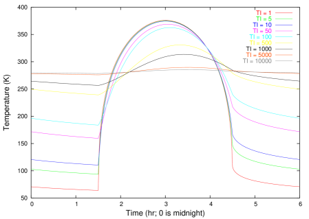
Figure 2: Synthetic diurnal temperature curves on the equator of a model asteroid for different values of thermal inertia (in units of J s -1/2 K -1 m -2). Increasing thermal inertia smooths temperature contrasts and additionally causes the temperature peak to occur after the insolation peak at $3\text{\,}\mathrm{h}$. The asteroid is situated at a heliocentric distance of $r=$1.1\text{\,}\text{AU}$$, has a spin period of $6\text{\,}\mathrm{h}$, a Bond albedo of $A=0.1$, and its spin axis is perpendicular to the orbital plane.

Table 1: Thermal inertia: Some familiar examples.

Noon

The hottest time of day is generally after noon, and the hottest time of the year is generally after the summer solstice due to thermal inertia.

Oceanic and continental climate

The thermal inertia of water greatly exceeds that of soil. Consequently, the climate close to oceans or large lakes is generally mild, with moderate temperature differences between both day and night or summer and winter. This is contrasted by continental climate as in, e.g., central Siberia, with hot summers but notoriously extreme winters.

Earth and Moon

Although the Moon is at the same heliocentric distance as the Earth, lunar temperatures oscillate between around $100\text{\,}\mathrm{\SIUnitSymbolCelsius}$ at day time and some $-150\text{\,}\mathrm{\SIUnitSymbolCelsius}$ at night. This is caused by the extremely low thermal inertia of its regolith-dominated surface together with the low spin rate.

See sect. 2 for a formal definition of thermal inertia and a mathematical discussion, table 1 for some familiar examples and sect. 8 for a discussion of what is known about asteroid thermal inertia and physical implications thereof.

In asteroid observations at low phase angles (as typical for MBAs and objects in the outer Solar System), the chief effect of thermal inertia is a reduction of the day-time temperature relative to a low-thermal-inertia object, hence a reduction in absolute flux level and also in apparent color temperature (i.e. the observed flux is skewed towards longer wavelengths). The enhanced emission from the night side does not contribute significantly to the observable flux since most parts of the non-illuminated hemisphere are not visible at low phase angles. The effect of thermal inertia on large-phase-angle observations, such as typical NEA observations, is less straightforward to predict and generally requires careful modeling.

On asteroids, thermal inertia is caused by thermal conduction into and from the subsoil. Large asteroids are well known to be covered with dusty regolith, which is a poor thermal conductor, hence their thermal inertia is very low (see sect. 2 for a discussion). Generally, neglecting their thermal inertia does not introduce large systematic diameter uncertainties.

Little is known, however, about the thermal inertia of small asteroids including NEAs (see sect. 8), therefore one is ill advised to neglect their thermal inertia. Also, NEAs are regularly observed at much larger solar phase angles (see sect. 5), where the effects of thermal inertia become more pronounced. In the interpretation of thermal NEA data, it is therefore crucial to take thermal inertia into account to avoid significant systematic diameter uncertainties.

The effect of thermal inertia is tightly coupled to the rotational properties: A slow rotator with high thermal inertia may mimic the diurnal temperature curve of an otherwise identical fast rotator of low thermal inertia (see eqn. 10c on p. 10c). Also, the spin axis orientation is important: Obviously, the diurnal temperature distribution on an object whose spin axis points towards the Sun shows no effect of thermal inertia whatsoever; thermal inertia has the most profound influence on the diurnal temperature distribution if the subsolar point is at the equator.

3 Beaming due to surface roughness

By comparing thermal diameters with occultation diameters, STM and LebofskySpencer1989 found what appeared to be a systematic thermal-flux surplus at low phase angles: Thermal emission is “beamed” into the sunward direction, such that at low phase angles a larger-than-expected flux level is observable at an elevated apparent color temperature. This effect is referred to as thermal-infrared beaming.

Like the well-known optical opposition-effect (see, e.g., BelskayaShevchenko2000), thermal-infrared beaming is thought to be caused by surface roughness. Imagine a hemispherical crater at the subsolar point, where the solar incidence vector coincides with the crater symmetry axis. Inside the crater, surface elements can exchange energy radiatively leading to mutual heating due both to sunlight scattered inside the crater and due to reabsorption of thermal emission. Relative to an equally-sized, flat surface patch, the crater therefore absorbs a larger amount of energy and thermally emits at an elevated effective temperature. Furthermore, craters situated off the subsolar point contain surface elements which point towards the Sun (and, at low phase angle, to the observer). This reduces the amount of thermal limb darkening relative to a Lambertian emitter.

Due to conservation of energy, one would expect a reduced color temperature and reduced flux level at larger phase angles. In particular, beaming would be expected to lead to a phase-angle dependence of the apparent color temperature (see sect. 2 for a further discussion).

4 Shape and spin state

While large MBAs generally tend to be nearly spherical, smaller asteroids display a large diversity of shape (see sect. 4) which, combined with their spin, typically causes their projected visible area to vary with time. This induces a time variability in optical brightness (optical lightcurve) and also in thermal emission (thermal lightcurve), typically with two peaks per asteroid revolution, such that the lightcurve period equals half the spin period. The lightcurve amplitude depends on the asteroid shape, on the phase angle of the observations, and also on the aspect angle (Zappala1990). It may be larger than one magnitude for extremely elongated objects, corresponding to a minimum-to-maximum flux variability of a factor around 2.5.

It is important to take account of the rotational thermal-flux variability when deriving diameters. Failure to do so not only introduces an unpredictable diameter offset but might also cause the estimated color temperature to be flawed (typically, spectrophotometric observations in different filters are not taken simultaneously). If the shape of the object is known, a detailed thermophysical model (see chapter 3) can be used to exploit this information. Typically, however, the shape is unknown and only a few thermal data-points are available, typically insufficient to trace the thermal lightcurve. In that case, thermal data are often “lightcurve-corrected” on the basis of optical lightcurve data, which are typically more readily available.

However, optical and thermal lightcurve may differ in phase and/or structure due to the effects of shape, surface structure, thermal inertia, or albedo variegation. While this may cause uncertainties for lightcurve correction of thermal flux values to derive diameters using thermal models based on spherical shape, these lightcurve effects can often be exploited to determine the thermal inertia using a thermophysical model. LebofskyRieke1979, e.g., observed a phase shift between thermal and optical lightcurve data of (433) Eros which they explained in terms of a temperature lag due to thermal inertia (see sect. 1); Lellouch2000 report a similar phase lag in the thermal lightcurve of (134340) Pluto.

5 Observation geometry

It is clear that observed thermal fluxes depend critically on the observing geometry: Fluxes scale with $\Delta^{-2}$ (observer-centric distance $\Delta$), the absorbed solar energy scales with $r^{-2}$ (heliocentric distance $r$). Objects in the outer Solar System are therefore much colder than bodies in near-Earth space and consequently their thermal emission peaks at much longer wavelengths.

Solar elongation

The practical observability of asteroids is typically determined by their solar elongation, i.e. their angular distance from the Sun as seen by the observer, together with their declination. Objects on the celestial equator at solar elongations below $90\text{\,}\mathrm{\SIUnitSymbolDegree}$ culminate on the day sky and are consequently difficult to observe from ground (see sect. 4 for solar-elongation constraints on observations with the Spitzer Space Telescope).

Solar phase angle

Closely related to the solar elongation is the solar phase angle, $\alpha$, which is of great importance for thermal modeling. Distant objects such as MBAs typically reach their peak brightness at opposition, when $\alpha\sim 0$ and the solar elongation is maximized (typically close to $180\text{\,}\mathrm{\SIUnitSymbolDegree}$)—this is different for near-Earth objects with reach their peak brightness around the date of closest approach.

Objects at large observer-centric distances can only be observed at relatively small phase angles whereas NEAs often sweep large ranges of phase angle within a few weeks during close approaches to Earth.

At low phase angles, the observed thermal flux is vastly dominated by the hot subsolar region; thermal inertia reduces both the observed flux level and the color temperature by transporting heat to the night side, from where it is not observable. For low thermal inertia, the temperature distribution is nearly symmetric about the subsolar point, which nearly coincides with the sub-observer point; due to this approximate symmetry, radiometric diameters are largely insensitive to the temperature distribution.

At large phase angles, however, large portions of the non-illuminated side become observable, rendering the observable thermal emission more sensitive to the details of the temperature distribution. The latter is determined by shape, thermal inertia, spin state, and surface roughness.

At low phase angles, the cooling effect of thermal inertia may be countered by the beaming effect due to surface roughness, which increases the apparent color temperature. At larger phase angles, however, also beaming is expected to lead to a cooling effect, making it difficult to disentangle the two effects.

Accurate derivation of thermal properties such as thermal inertia hence typically requires observations at several phase angles.

Aspect angles

Also important are the aspect angles, chiefly the subsolar and sub-observer latitude on the asteroid. These depend on the asteroid spin axis, which is often unknown. Lightcurve effects and the effect of thermal inertia are maximized when the spin axis is perpendicular to the viewing plane (i.e. when both the subsolar and sub-observer point are on the equator), both effects are minimized if the asteroid is viewed pole-on.

6 Thermal emission model

The temperature-dependent spectral characteristics of asteroid thermal emission is typically modeled using a gray-body law, i.e.  a Planck black body with a spectrally constant emissivity $\epsilon$. The latter assumption is only approximately valid. There are well-known spectral features in the thermal infrared; those with the largest spectral contrast are due to silicates and located at wavelengths of 8–10 and $15--25\text{\,}\mathrm{\SIUnitSymbolMicro m}$. Not many thermal-infrared spectroscopic observations of asteroids have been published (see Lim2005; Emery2006, and references therein—see also sect. LABEL:sect:Patroclus), but the typical spectral contrast of detected features is only a few percent if spectra were detectable at all.

While the emissivity is roughly spectrally constant over the relevant wavelength range, the exact value of the bolometric emissivity is less well constrained. As is common practice, we assume $\epsilon=0.9$, which is a typical value for silicate powders known from laboratory measurements (see, e.g., HovisCallahan1966). Bolometric emissivities cannot exceed 1, and for most common materials, $\epsilon$ is within $10\text{\,}\%$ of 0.9; a notable exception are polished metal surfaces which can have emissivities down to a few percent (see, e.g., Berber1999, Tab. 29). To first order, asteroid thermal fluxes are proportional to $\epsilon D^{2}$, hence the emissivity uncertainty induces a fractional diameter uncertainty of $5\text{\,}\%$ at most—except for polished metallic objects, a very implausible asteroid surface model.

3 Observability

Figure 3: Atmospheric transmissivity as a function of wavelength over the summit of Mauna Kea/Hawai’i, one of the best sites for infrared observations. The clearly visible transmissive regions are called “atmospheric windows” and are named (with increasing wavelength) J, H, K, L, M, N, and Q; thermal-infrared windows are the M window ($\sim$5\text{\,}\mathrm{\SIUnitSymbolMicro m}$$), the N window ($\sim$10\text{\,}\mathrm{\SIUnitSymbolMicro m}$$), and the Q window ($\sim$20\text{\,}\mathrm{\SIUnitSymbolMicro m}$$). The atmospheric transparency model was developed by Lord1992, data were made available through the GEMINI website http://www.gemini.edu/sciops/ObsProcess/obsConstraints/ocTransSpectra.html (assuming $1\text{\,}\mathrm{mm}$ of precipitable water and an airmass of 1.5).

The thermal emission of asteroids peaks in the mid-infrared wavelength range (also referred to as thermal infrared), typically between 10 and $20\text{\,}\mathrm{\SIUnitSymbolMicro m}$. The thermal emission of outer-Solar-System objects peaks at larger wavelengths, beyond $50\text{\,}\mathrm{\SIUnitSymbolMicro m}$ in the case of Kuiper belt objects.

The atmosphere is mostly opaque in the thermal-infrared wavelength range and practically totally opaque at larger infrared wavelengths, chiefly due to absorption from $\text{CO}_{2}$ and $\text{H}_{2}\text{O}$. Ground-based observations of the thermal emission of outer-Solar-System bodies are therefore virtually impossible, while asteroid observations are restricted to “atmospheric windows” (see Fig. 3).

Further problems stem from the fact that thermal emission of, e.g., the atmosphere, clouds, or even the telescope mirrors cause high levels of rapidly varying background radiation; thermal-infrared detectors are typically cooled with liquid helium in order to minimize their own thermal emission. The large background level makes special observation techniques necessary, such as those discussed in sect. 3.

In the thermal infrared, it is therefore particularly advantageous to observe from a vantage point above most of the atmosphere (e.g. at the summit of a high mountain or in an airborne telescope) or above all of the atmosphere using a space telescope. The currently most sensitive imaging instruments in the thermal infrared are on board the Spitzer Space Telescope, although its aperture of $85\text{\,}\mathrm{cm}$ is much smaller than that of, e.g., the $10\text{\,}\mathrm{m}$ Keck-2 telescope.

A widely used unit of mid-infrared flux (monochromatic flux density) is W m µ m , also widely used is the Jansky (Jy); equals . Fluxes are converted from one unit into the other as follows:

$$F_{\text{Jy}}\left(\lambda\right)=F_{\mathrm{W}\rpsquare\mathrm{m}\reciprocal\mathrm{\SIUnitSymbolMicro}\mathrm{m}}\left(\lambda\right)\times\lambda_{\mathrm{\SIUnitSymbolMicro}\mathrm{m}}{}^{2}\times 0.33356\times 10^{12}$$ (3)

where the latter factor contains the reciprocal of the speed of light required to convert from flux per wavelength to flux per frequency.

4 Simple models: STM and FRM

In this section, two widely used, yet highly idealized, thermal models are described: The Standard Thermal Model (STM, see sect. 1), which neglects the combined effect of rotation and thermal inertia, and the Fast Rotating Model (FRM, see sect. 2), which effectively assumes an infinitely large thermal inertia.

Both models were developed in the 1970s, when thermal-infrared observations of asteroids were effectively limited to a single wavelength. The color temperature is fixed by the respective model assumptions, hence data at a single thermal wavelength are sufficient to estimate the diameter.

1 Standard Thermal Model (STM)

In the Standard Thermal Model (STM, see STM, and references therein), the asteroid is assumed to be spherical, to have a vanishing thermal inertia (hence its spin state is irrelevant), and to be observed at opposition, i.e. at a phase angle of $0\text{\,}\mathrm{\SIUnitSymbolDegree}$. Under these assumptions, conservation of energy determines the temperature at the subsolar point $T_{SS}{}$ of a smooth asteroid:

$$\epsilon\sigma T_{SS}{}^{4}=\left(1-A\right)\frac{S}{r^{2}}$$ (4)

where $\epsilon$ denotes the bolometric emissivity, $\sigma$ the Stefan-Boltzmann constant, $A$ the bolometric Bond albedo (see sect. 1), $S$ the solar constant, and $r$ is the heliocentric distance in AU. In the absence of thermal inertia, temperatures are in instantaneous equilibrium with insolation, and hence the temperature distribution on the surface solely depends on the angular distance from the subsolar point (or, equivalently, the angle formed by the solar incidence vector and local zenith) $\Phi$:

$$T\left(\Phi\right)=\begin{cases}T_{SS}{}\cos^{\frac{1}{4}}\Phi&\text{if}\ \Phi\leq$90\text{\,}\mathrm{\SIUnitSymbolDegree}$\\ 0&\text{otherwise (i.e.\ Sun is below local horizon)}\end{cases}$$ (5)

Using the Planck function

$$B\left(\lambda,T\right)=\frac{2\pi hc^{2}}{\lambda^{5}}\frac{1}{\exp\left[hc/\left(\lambda kT\right)\right]-1}$$ (6)

with the Planck constant $h$, velocity of light $c$, and Boltzmann constant $k$, the total flux $f(\lambda)$ at wavelength $\lambda$ then equals

$$f(\lambda)=\frac{\epsilon D^{2}}{2\Delta^{2}}\int\limits_{0}^{\pi/2}B\left(\lambda,T\left(\Phi\right)\right)\sin\Phi\cos\Phi\text{d}\Phi.$$ (7)

The symmetry about the subsolar point renders the azimuthal integral trivial, leaving only a one-dimensional integral to be performed numerically.

The STM assumes observations to take place at opposition, whereas real observations typically occur at $\alpha>0$, requiring a phase-angle correction. LebofskySpencer1989 employ an empirical phase coefficient of $0.01\text{\,}\text{mag}\mathrm{/}\text{degree}$, which was found by Matson1971 to be a good approximation to the phase curve of asteroids observed at N-band wavelengths and at phase angles up to $30\text{\,}\mathrm{\SIUnitSymbolDegree}$. It must be emphasized that the STM is not applicable at larger phase angles.

STM and LebofskySpencer1989 found that diameters estimated using this “naive” STM were systematically larger than estimates derived using other techniques, which they attributed to thermal-infrared beaming (see sect. 3). As a first-order correction, the so-called beaming parameter $\eta$ was introduced into the energy balance (eqn. 4)

$$\epsilon\sigma\boldsymbol{\eta}T_{SS}{}^{4}=\left(1-A\right)\frac{S}{r^{2}}.$$ (8)

$\eta<1$ enhances the model temperature and thus the expected flux level (thereby reducing model diameters required to match measured fluxes) while $\eta>1$ reduces both the temperature and flux level. By comparing occultation diameters of the few largest MBAs to radiometric diameters, they determined a best-fit “canonical” value of $\eta=0.756$. The thus modified STM is widely used, and frequently referred to as the “refined” STM to distinguish it from the case $\eta=1$.

The STM was designed to interpret single-wavelength measurements; there is only one free parameter, namely the diameter $D$ (the albedo $A$ which appears in eqn. 8 is linked to $D$ through the optical magnitude $H$, see sect. 1). When, however, observations at more than one wavelength are available, it is common practice to derive one diameter value per data point and to compare the diameters. They are then often referred to by the used wavelength, e.g. as “N-band diameter” or “Q-band diameter.”

For large MBAs, it was found that STM-derived diameters typically agree well with estimates derived using other techniques. Much less is known about smaller asteroids including NEAs. The STM was used to derive the largest currently available catalog of asteroid diameters and albedos (IRAS; SIMPS) from data obtained with the InfraRed Astronomy Satellite (IRAS).

2 Fast Rotating Model (FRM)

An alternative, equally simple model was devised by LebofskyBetulia, called the Fast Rotating Model (FRM) or Isothermal Latitude Model (ILM). In this model, the diurnal temperature distribution is constant for regions of constant geographic latitude. This corresponds to the assumption of infinitely fast rotation about a spin axis perpendicular to the observing plane spanned by the Sun, the observer and the asteroid; the often-made assertion that the FRM assumes an infinite thermal inertia is not strictly valid since it neglects lateral heat conduction, which would cause the asteroid to become isothermal. Nevertheless, the FRM should be more appropriate for high-thermal-inertia asteroids than the STM.

The FRM was developed in the late 1970s to explain the discrepancy in different diameter estimates for the NEA (1580) Betulia, for which the STM diameter was found to be much lower than estimates resulting from radar and polarimetric observations (LebofskyBetulia, see also sect. 3). Using the FRM rather than the STM resolved the apparent discrepancy, hence it was concluded that Betulia had a very high thermal inertia consistent with a surface of bare rock.

Under the FRM assumptions, a strip at geographic latitude $\theta$ (width $D/2\ \text{d}\theta$) is in thermal equilibrium with the absorbed sunlight averaged over one rotation:

$$\left(\pi\frac{D^{2}}{2}\cos\theta\text{d}\theta\right)\epsilon\sigma T^{4}=\frac{(1-A)S}{r^{2}}\cos\theta\left(\frac{D^{2}}{2}\cos\theta\text{d}\theta\right)$$ (9)

(energy is emitted from a total area of $\pi D^{2}/2\ \cos\theta\text{d}\theta$ and absorbed on a total projected area of $D^{2}/2\ \cos\theta\text{d}\theta$, the second factor of $\cos\theta$ on the right-hand side of eqn. 9 is for the solar incidence angle). The temperature distribution equals

$$T\left(\theta\right) =T_{SS}{}\cos^{\frac{1}{4}}\theta$$ (10)

$$T_{SS}{} =\left(\frac{S}{r^{2}}\frac{1-A}{\pi\epsilon\sigma}\right)^{\frac{1}{4}}.$$ (11)

Note that eqn. 11 formally corresponds to eqn. 8 with $\eta=\pi$; thermal inertia carries energy from the day side towards the night side, hence the former is much cooler than in the STM case. The total model flux equals

$$f(\lambda)=\frac{\epsilon D^{2}}{\pi\Delta^{2}}\int\limits_{0}^{\pi/2}B\left[\lambda,T\left(\theta\right)\right]\cos^{2}\theta\text{d}{\theta}.$$ (12)

Due to the rotational symmetry of the temperature distribution, FRM fluxes do not depend on solar phase angle, hence no phase-angle correction is required. One might therefore expect the FRM to be a more appropriate model than the STM for observations of high-thermal-inertia objects at large phase angles.

5 Near-Earth Asteroid Thermal Model (NEATM)

In the STM and the FRM described in 4, the temperature distribution on the asteroid surface as well as the maximum temperature are completely determined by the model, where very different assumptions are made on thermal properties. In general, neither model provides a good fit to the measured spectral emission properties of small asteroids such as NEAs. NEATM proposed a modified variant of the STM, the Near-Earth Asteroid Thermal Model (NEATM), in which the model temperature scale is adjusted to fit the observed data, enabling a first-order correction to effects of thermal inertia, surface roughness, or shape. This requires spectrophotometric data at two or more thermal wavelengths and enables some information on thermal properties to be obtained (see sect. 2) in addition to estimates of diameter and albedo which are generally more accurate than those based on simpler thermal models such as the STM or FRM (this will be discussed in sect. 3). In sect. 4 we describe our fitting routine, which is used mutatis mutandis also for thermophysical model fitting.

Despite its name, the NEATM is suitable for application to thermal data from any atmosphereless body, not only NEAs. In this work, thermal-infrared data of various asteroids are fitting using the NEATM (most data are also fitted using the thermophysical model described in chapter 3).

1 Model description

Like the STM, on which it is based, the NEATM assumes a spherical asteroid shape with an STM-like temperature distribution (eqn. 5 and eqn. 8). In contrast to the STM, however, the parameter $\eta$ no longer has a fixed value. Rather, $\eta$ is varied in order to match the spectral distribution of the observed data, i.e. the apparent color temperature; the physical significance thereof will be discussed in sect. 2. Furthermore, in contrast to the STM, where observations are assumed to take place at opposition and observed data are phase-angle corrected using an empirical phase coefficient, NEATM fluxes are calculated at the phase angle $\alpha$ at which the observations took place assuming Lambertian emission. To this end, a two-dimensional integral is performed over that part of the sphere which is illuminated and visible to the observer. In a spherical coordinate system with the subsolar and sub-observer points at the equator ($\theta=0$) and azimuth angle $\phi=0$ at the subsolar point (the sub-observer point is at $\phi=\alpha$):

$$f\left(\lambda\right)=\frac{\epsilon D^{2}}{\Delta^{2}}\int\limits_{0}^{\pi/2}\text{d}\theta\int\limits_{-\frac{\pi}{2}+\alpha}^{\frac{\pi}{2}+\alpha}\text{d}\phi\ B\left[\lambda,T\left(\theta,\phi\right)\right]\ \cos^{2}\theta\ \cos\left(\phi-\alpha\right)$$ (13)

(the factor $\cos\theta\cos(\phi-\alpha)$ is the cosine of the observer angle, a second factor $\cos\theta$ stems from the surface element $\text{d}A=\cos\theta\text{d}\theta\text{d}\phi$) with

$$T(\theta,\phi)=\begin{cases}T_{SS}{}\cos^{\frac{1}{4}}\theta\cos^{\frac{1}{4}}\phi&\text{for}\cos\theta\cos\phi\geq 0\\ 0&\text{otherwise (Sun below local horizon)}\end{cases}$$ (14)

and (see eqn. 8)

$$\epsilon\sigma\eta\ T_{SS}{}^{4}=\frac{(1-A)S}{r^{2}}.$$ (15)

The NEATM contains two free parameters to fit the data: the diameter $D$ (from which the bolometric Bond albedo $A$ is calculated) and the model parameter $\eta$. Thermal measurements $f_{i}(\lambda_{i})$ at two or more well spaced thermal wavelengths are required for meaningful NEATM fits.

2 Physical significance of $\boldsymbol{\eta}$

Figure 4: NEATM spectra of a model asteroid with $\eta=0.8$, $\eta=1.2$, and $\eta=2.5$. Remaining model parameters are: $H=16$, $G=0.15$, $p_{\text{V}}{}=0.2$, $r$ = , $\Delta=$0.1\text{\,}\text{AU}$$, $\alpha=$20\text{\,}\mathrm{\SIUnitSymbolDegree}$$, and $\epsilon=0.9$.

The value of $\eta$ scales the subsolar temperature $T_{SS}{}$ (eqn. 15) and hence the temperature throughout the surface (eqn. 14), where $\eta=1$ corresponds to a smooth zero-thermal-inertia (Lambertian) surface, $\eta<1$ corresponds to a globally elevated temperature, while $\eta>1$ corresponds to a reduced temperature. Varying $\eta$ therefore allows the model spectrum to be fitted to the spectral distribution (apparent color temperature) of the observed data (see 4 for a schematic example). No such mechanism to match the observed color temperature is available in simpler models such as the STM or FRM, hence NEATM-derived diameters may be expected to be more accurate (see sect. 3). In particular, NEATM spectra with low $\eta$ values around the “canonical” STM value of $\eta=0.756$ mimic STM spectra (the agreement is identical at $\alpha=0$), while NEATM values for large $\eta$ values above $\sim 2.5$ tend towards FRM spectra (see Fig. 4); in a way, therefore, the NEATM interpolates between those two extreme models.

$\eta$ is a measure of the apparent color temperature, from which conclusions can be drawn on the physical temperature and hence on thermal properties. As described in sect. 5, thermal inertia and surface roughness alter the apparent color temperature, depending on the solar phase angle $\alpha$ at which the observations took place. One may therefore expect $\eta$ determinations at different phase angles to contain information about thermal inertia and thermal-infrared beaming.

Figure 5: Observed NEATM model parameter $\eta$ as a function of phase angle $\alpha$ for an ensemble of NEAs. Most asteroids have been observed only once, but there are, e.g., 5 data points for (5381) Sekhmet. (Data compiled in Delbo2007, see references therein)

Delbo2007 compiled $\eta$ values from all currently published multi-wavelength spectrophotometric NEA observations of sufficient data quality (see Fig. 5). There is a clear correlation between $\eta$ and $\alpha$, which is probably due to infrared beaming. The conspicuous lack of large $\eta$ values at low phase indicates that most NEAs in this ensemble do not have a large thermal inertia indicative of a bare-rock surface (Delbo2003), with the four (or five) objects displaying the largest $\eta$ values possibly being exceptions. An ensemble-average thermal inertia of these NEAs was determined by fitting the distribution of $\eta$ values using a detailed thermophysical model similar to that described in chapter 3 (Delbo2007).

3 Accuracy of NEATM-derived diameters and albedos

The systematic uncertainty about the validity of the model assumptions inherent to the NEATM translate into systematic uncertainties of determined diameters and albedos, where the systematic fractional albedo uncertainty is twice that of the fractional diameter uncertainty by virtue of eqn. 1. In many practical cases, other sources of uncertainty such as statistical and systematic flux uncertainties or uncertainties caused by the lightcurve-correction procedure (or lack thereof) can be neglected relative to the systematic diameter uncertainty. Additionally, the uncertainty in absolute optical magnitude $H$ contributes towards the albedo uncertainty.

In the case of large MBAs, STM-derived diameters are known to be in good agreement with occultation diameters, with a relative deviation of $11\text{\,}\%$ for a sample of 12 MBAs of low lightcurve amplitude (where the two diameter estimates can be compared readily; see HarrisLagerros2002, and references therein). At the small phase angles at which MBAs are observed, the NEATM and the STM produce generally very similar model predictions provided that the best-fit $\eta$ value is not large (which is generally the case for large objects, see Walker2003).

Comparison of NEATM diameters and albedos of NEAs with other results

In the case of small asteroids including NEAs, assessment of the systematic diameter and albedo accuracy is hampered by the scarcity of “ground truth” data for comparison. Since the work of Veeder1989 it is known that there is significant systematic uncertainty in NEA diameters if only the STM and FRM are considered. Multi-wavelength spectrophotometry analyzed using the NEATM effectively allows one to interpolate between those two extreme models but is still sufficiently simple to be applicable in the absence of detailed a priori information on the target (given which more detailed modeling is preferable).

HarrisLagerros2002 quote STM, FRM, and NEATM diameters and albedos for a sample of 20 NEAs and conclude that generally NEATM results are in better agreement with albedos expected on the basis of taxonomic classification (see sect. 2) or spacecraft imaging (in the case of 433 Eros).

While no occultation diameters of NEAs have been published, radar measurements can provide very accurate estimates of NEA diameters. Delbo2004 compare radiometric diameters with radar-derived diameters for all NEA data available at that time. He finds the rms. deviation between NEATM and radar diameters of the considered NEAs to be around $20\text{\,}\%$.

It is often quoted (see, e.g., WT24) that comparison of NEATM results with results from other sources, such as radar, indicate that the overall systematic uncertainty is less than $15\text{\,}\%$ in diameter and $30\text{\,}\%$ in albedo, but uncertainties may be larger in the case of very elongated or highly irregularly shaped objects and/or for observations at very large phase angles when night-side emission (which is neglected in the NEATM) becomes more relevant.

Mutual comparison of thermal and thermophysical models

It is instructive to check the NEATM against other thermal models, particularly against detailed thermophysical models. Although it must be cautioned that also the latter carry systematic uncertainties which are currently not well explored, such studies may reveal systematic offsets of NEATM diameters as a function of, e.g., thermal inertia or phase angle of observations.

Harris2006 used NEATM to fit synthetic thermal flux values, which were generated using a thermophysical model including the effects of thermal inertia but without surface roughness. He showed that for $\alpha<$50\text{\,}\mathrm{\SIUnitSymbolDegree}$$ and thermal inertia below some $500\text{\,}\mathrm{J}\usk\power{\mathrm{s}}{-1/2}\power{\mathrm{K}}{-1}\power{\mathrm{m}}{-2}$, NEATM-derived diameters were within $15\text{\,}\%$ of the input diameter. In a similar analysis, Wright2007 found that the NEATM reproduces the input diameter to within $10\text{\,}\%$ (r.m.s.) for $\alpha<$60\text{\,}\mathrm{\SIUnitSymbolDegree}$$ for a particular model of surface roughness and different thermal inertia values. None of these analyses considered the effect of irregular shape beyond cratering, where the latter is neglected in Harris’ analysis.

4 NEATM fitting routine

In the course of this thesis work, a NEATM model code was implemented in C++, independent of that by NEATM or Delbo2004. Model fluxes from all three implementations were found to agree with one another except for negligible numerical noise. Also a fitting routine was developed, different from those by Harris or Delbo’ but leading to identical results; since this fitting routine is used mutatis mutandis also for our thermophysical model, it shall here be described in some detail.

Given $n$ data points $d_{i}(\lambda_{i})$ observed at wavelength $\lambda_{i}$ and their uncertainties $\sigma_{i}$, we aim at minimizing

$$\chi^{2}=\sum_{i=1}^{n}\frac{\left[m_{i}(\lambda_{i})-d_{i}(\lambda_{i})\right]^{2}}{\sigma_{i}^{2}}$$ (16)

where the model fluxes $m_{i}(\lambda_{i})$ are determined from eqn. 13 with parameters

• Observing geometry: $r$, $\Delta$, $\alpha$

• Asteroid constants: $H$, $G$, $\epsilon$

• NEATM fit parameters: $\eta$ and either $D$ or $p_{\text{V}}{}$.

In our fitting routine, $\eta$ and the geometric albedo $p_{\text{V}}{}$ are varied; the factor $D^{2}$ in eqn. 13 is proportional to $1/p_{\text{V}}{}$ by virtue of eqn. 1. The $\eta$ axis of the parameter space is searched for the minimum $\chi^{2}{}$ longward of $\eta=0.6$ (implicitly assuming that $\eta$ values below 0.6 are unphysical) at a step width of 0.4 in $\eta$. For each $\eta$ value, the best-fit $p_{\text{V}}{}$ value and corresponding $\chi^{2}{}$ are determined until the minimum in $\chi^{2}$ is boxed, i.e. until a series of three consecutive $\eta$ values is found for which the middle value leads to the lowest of the three $\chi^{2}$ values. Then the best-fit $\eta$ value is determined using a bisection algorithm.

The best-fit $p_{\text{V}}{}$ for constant $\eta$ is determined iteratively. To this end, NEATM fluxes are calculated using a seed value of $p_{\text{V}}{}_{0}$ (usually 0.2, but this value can be changed for debugging). Using linear regression, we determine a scale factor $\kappa$ (see eqn. 17) which leads to the best fit of the model fluxes with the data without changing the color temperature. Following iterations assume the $p_{\text{V}}{}$ value of their predecessor divided by the thus obtained $\kappa$ value. This is repeated until $p_{\text{V}}{}$ stabilizes to a user-defined fractional accuracy goal.

If temperatures were independent of $p_{\text{V}}{}$, the integrand in eqn. 13 would be independent of $p_{\text{V}}{}$ and thermal fluxes would be proportional to $1/p_{\text{V}}{}\propto\kappa$ for constant $H$, hence the iteration above would converge to the exact result in the first step. In reality, temperatures are a weak function of $p_{\text{V}}{}$, hence the iteration typically converges after a small number of iterations. The convergence velocity improves with increasing number of data points and with decreasing albedo. We observed that in most cases we over-correct $p_{\text{V}}{}$, i.e. that $\kappa>1$ is typically followed by $\kappa<1$ in the next iteration, and vice-versa. Sometimes this behavior leads to stable oscillations so the algorithm does not converge. To prevent this, we update $p_{\text{V}}{}$ by dividing by $\sqrt{\kappa}$ rather than $\kappa$, and by $\sqrt[4]{\kappa}$ if $p_{\text{V}}{}\geq 0.5$. This has led to stable convergence in all cases so far.

Determining the best-fit $\mathbf{p_{\text{V}}{}}$ for constant $\boldsymbol{\eta}$

It is assumed that fluxes are nearly proportional to $1/p_{\text{V}}{}$ and thus to $\kappa$. Eqn. 16 then reads:

$$\chi^{2}=\sum_{i}^{n}\frac{\left[\kappa\ m_{i}(\lambda_{i})-d_{i}(\lambda_{i})\right]^{2}}{\sigma_{i}^{2}}=:\kappa^{2}MM-2\kappa MD+DD$$ (17)

with

$$MM :=\sum_{i}^{n}\left(\frac{m_{i}(\lambda_{i})}{\sigma_{i}}\right)^{2}$$ (18a)

$$MD :=\sum_{i}^{n}\frac{m_{i}\left(\lambda_{i}\right)d_{i}\left(\lambda_{i}\right)}{\sigma_{i}^{2}}$$ (18b)

$$DD :=\sum_{i}^{n}\left(\frac{d_{i}(\lambda_{i})}{\sigma_{i}}\right)^{2}.$$ (18c)

The sums $MM$, $MD$, and $DD$ can be calculated in a numerically efficient way after model fluxes have been calculated; in particular, model fluxes need not be stored in memory. The best-fit value of $\kappa$ satisfies $\text{d}\chi^{2}/\text{d}\kappa=0$, i.e. $\kappa=MD/MM$.

Chapter 3 Detailed thermophysical modeling

A detailed thermophysical model (TPM) is presented which is applicable to all asteroids including NEAs. The effects of thermal inertia, spin state, irregular shape, and thermal-infrared beaming are explicitly taken into account. Arbitrary convex shapes are allowed for, a generalization to non-convex shapes is under development (see chapter LABEL:chapt:TPMconcave in the appendix).

Realistic thermophysical modeling is required in order to reach the primary goal of this thesis, namely to determine the thermal inertia of NEAs through analysis of thermal-infrared observations; we wish to emphasize that there is no other well-established method of measuring the thermal inertia of asteroids. Furthermore, since the thermal physics of asteroid surfaces is here modeled in a more realistic way than in the highly idealized thermal models described in the previous chapter, TPM-derived estimates on diameter and albedo are potentially more accurate.

The thermal emission of NEAs is more challenging to model than that of MBAs due to their larger thermal inertia and because they are typically observed at much larger solar phase angles. While TPMs applicable to MBA data have previously been available, we here report the first TPM shown to be applicable to NEA data.

After an overview section, the thermal physics of asteroid surfaces is discussed in sect. 2. The model implementation is presented in sect. 3, validation test are presented in sect. 4. Sect. 5 is devoted to fitting techniques.

1 Overview

Various models have been proposed to overcome the limitations of simple thermal models. E.g., Hansen1977 proposed a physical model for asteroid surface roughness along with an approximative treatment of conduction on a spherical asteroid. Non-spherical asteroid shapes have been modeled by Brown1985, who proposed a variant of the STM with ellipsoidal asteroid shape. Spencer1990 proposed an improved variant of Hansen1977’s model in which thermal conduction is modeled in more detail. A variant of Spencer1990’s model has been used by Delbo2004. The most realistic asteroid TPM currently available is that by LagerrosI; LagerrosIII; LagerrosIV in which thermal conduction and surface roughness are explicitly modeled on an asteroid of arbitrary shape. The Lagerros TPM has been widely used and is well tested for applications to large MBAs. It enabled their thermal emission to be studied to such a high accuracy that they are used as calibration standards for space telescopes (see, e.g., MuellerLagerros1998; MuellerLagerros2002).

TPMs for asteroids were largely inspired by observations and models of other atmosphereless bodies. The first extraterrestrial body with well understood thermal properties was the Moon. It was found to display a thermal-infrared beaming effect by PettitNicholson1930 who also concluded that the thermal conductivity of lunar regolith was extremely low (see also Wesselink1948). Around the Apollo era the thermal properties of the Moon were studied in great detail from ground-based observations, in-situ measurements, and laboratory analysis of returned lunar samples (see, e.g., Buhl; WinterKrupp1971; Saari1972; Jones1975; Langseth1976, and references therein). While Martian results are not directly applicable to asteroids due to Mars’ atmosphere, lessons can be learned from spacecraft observations of Martian satellites (see, e.g., Lunine1982; Kuehrt1992), which are thought to be captured asteroids. Also Mercury is an atmosphereless body with a well observable and well modeled beaming effect (Emery1998). Due primarily to its slow spin, only the vicinity of Mercury’s terminator is expected to be influenced appreciably by thermal inertia. No effects of thermal conduction on Mercury could be found from ground-based observations, but thermal-infrared spacecraft observations using the MERTIS instrument (Benkhoff2006) on BepiColombo are to be expected in the future.

Our TPM is based on that by LagerrosI; LagerrosIII; LagerrosIV. Minor improvements to the physical modeling are proposed. The implementation is completely independent of Lagerros’. The model code was verified to produce physical results for very large solar phase angles and for a thermal inertia up to that of bare rock; extensive tests are reported in sect. 4. No such tests of the Lagerros TPM have been reported, but it is clear that his model was primarily aimed at application to MBAs. For geometric reasons, ground-based observations of MBAs cannot be performed at phase angles largely exceeding $30\text{\,}\mathrm{\SIUnitSymbolDegree}$. Furthermore, the typical thermal inertia of MBAs appears to be comparable to that of lunar regolith. For both reasons, modeling the thermal emission of MBAs is numerically less challenging than that of NEAs.

Our model is implemented in an object-oriented way (in C++) which makes it easy to add new features.

1 Model description

The asteroid is modeled as a convex mesh of typically a few thousand triangular facets. It is assumed to rotate about a fixed axis, i.e. non-principal-axis rotation (“tumbling”) is not supported. All physical surface properties, such as albedo, emissivity, thermal inertia, and surface roughness are assumed to be constant over the surface. Local surface temperatures are calculated from the local insolation geometry. One-dimensional thermal conduction into and from the subsoil is taken into account, all relevant parameters are assumed to be constant. To model surface roughness, model craters in the form of subdued hemispheres are added. The crater density and opening angle can be varied. Inside craters, shadowing, multiple scattering of optical and thermal flux, and reabsorption of both are fully taken into account, leading to thermal-infrared beaming.

Global-scale convexity

The asteroid shape model is assumed to be convex, only small-scale concavity is modeled in terms of craters. Global-scale convexity implies that facets cannot shadow one another, neither can they exchange energy radiatively which would lead to mutual heating. Since facets are typically very large compared to the penetration depth of the diurnal heat wave (see sect. 2), lateral heat conduction between facets can be neglected. Hence, the thermal flux emanating from an individual facet can be calculated independent of all other facets, which significantly simplifies the numerical treatment. A more general model variant, in which non-convex shape is allowed for, is described in chapter LABEL:chapt:TPMconcave in the appendix.

Most available models of asteroid shapes are convex by design (see Kaasalainen2002, for a review). Lacking such a shape model, one typically assumes a spherical or ellipsoidal shape, which are also convex.

2 Model parameters

Required asteroid parameters are the shape and spin state (see sect. 1 for details), the absolute optical magnitude $H$, slope parameter $G$, and emissivity $\epsilon$. Model variables are the geometric albedo $p_{\text{V}}{}$ (which determines the diameter $D$ through $H$, and furthermore the Bond albedo $A$), the thermal inertia in SI units ( J s -1/2 K -1 m -2), and the crater density and opening angle (in degrees). Model fluxes are calculated for a given Julian date, wavelength (in µ m ), and observing geometry, where the latter is defined by the heliocentric and observer-centric asteroid position in ecliptic coordinates (ecliptic longitude and latitude in degrees, distance in AU). Data taken at different epochs should be stored in separate fit files, but they can be read in and fitted simultaneously. Our techniques to fit model parameters to a given set of data are described in sect. 5.

3 Implementation overview

The TPM program takes .convex files as input. Those are generated using auxiliary programs based on computer-readable shape models (see sect. 1). On each facet, the diurnal temperature distribution is calculated as described in sect. 2. Thermal-infrared beaming is modeled as described in sect. 3. Disk-integrated model fluxes are calculated by summing up contributions from all visible facets.

2 Thermal physics

1 Global shape and spin state

In our TPM, the asteroid shape is modeled as a mesh of typically a few thousand planar triangular facets, the typical format of available asteroid shape models. The shape is defined by the coordinates of $n$ vertices which form $2n-4$ facets, each defined by the three indices of its vertices. As is common practice, a body-centric coordinate system is used in which the $z$ axis corresponds to the spin axis; non-principal-axis rotation (“tumbling”) is not supported so far. To model spherical and ellipsoidal shapes, an auxiliary program was developed which produces models of triangulated spheres of user-specified resolution and stretches them into ellipsoids if desired.

Geometric and thermal model tasks are separated in the code as far as possible, such that time-consuming geometric calculations need to be performed only once per shape. To this end, auxiliary programs have been developed to convert shape model files provided by colleagues (currently, the quasi-standard OBJ wavefront format and Mikko Kaasalainen’s variant thereof are supported) into a specifically defined type called .convex. For the thermal emission of convex asteroids the vertex positions are irrelevant, hence .convex files contain solely a list of $2n-4$ outbound surface-normal vectors (see sect. 1) and the model’s intrinsic diameter (see sect. 1). Shape models are not checked for convexity, they are assumed to be convex.

Outbound surface-normal vector

Each facet is defined by three vertex vectors $\vec{v_{1,2,3}}$ and has an outbound surface-normal vector (normal to the facet with a modulus equal to the facet size)

$$\vec{\text{d}\mathcal{A}}=\pm\frac{1}{2}\left(\vec{v_{2}}-\vec{v_{1}}\right)\times\left(\vec{v_{3}}-\vec{v_{1}}\right)$$ (1)

where $\times$ denotes the vector product. We calculate $\vec{\text{d}\mathcal{A}}$ with the positive sign and then check the orientation; the sign is flipped if the resulting vector is inbound. Assuming that the origin of the coordinate system is inside the object (which is true for all common distributions of shape models), $\vec{\text{d}\mathcal{A}}$ is outbound if

$$\vec{\text{d}\mathcal{A}}\cdot\frac{\vec{v_{1}}+\vec{v_{2}}+\vec{v_{3}}}{3}>0$$

(note that the division by 3 is not required to perform this test and is therefore not done in the code).

Intrinsic diameter

So far, all linear dimensions are in unspecified units. To convert them into physical units, they must be multiplied with a scale factor

$$s:=\frac{D_{\text{phys}}}{D_{\text{intr}}}$$ (2)

where $D_{\text{phys}}$ is the physical diameter determined from the constant $H$ and the variable $p_{\text{V}}{}$ (eqn. 1), and $D_{\text{intr}}$ is the intrinsic diameter of the shape model in unspecified units. As is common practice, the effective diameter is defined as that of the sphere of identical volume (see eqn. 1 on p. 1). The total volume $V$ of the polyhedral shape model equals the sum of all tetrahedral volumes $V_{i}$ defined by the origin and the three vertices $\vec{v_{i,123}}$ belonging to facet $i$

$$V =\sum_{i}\frac{1}{6}\left|\left(\vec{v_{i,1}}\times\vec{v_{i,2}}\right)\cdot\vec{v_{i,3}}\right|$$ (3a)

$$D_{\text{intr}} =\sqrt[3]{\frac{6V}{\pi}}.$$ (3b)

The scale factor $s$ is updated inside the TPM code whenever the variable $p_{\text{V}}{}$ is updated.

Transformation into a co-rotating system

For the calculation of model fluxes, the coordinates of the Sun, $\vec{e_{S}}{}$, and of the observer, $\vec{e_{O}}{}$, in a co-rotating asteroid-centric coordinate system are required. They are calculated from the epoch of the observation, $t$, and from the ecliptic coordinates of the asteroid in heliocentric $\left(\lambda_{S},\beta_{S}\right)$ and observer-centric $\left(\lambda_{O},\beta_{O}\right)$ frames, respectively, which are typically taken from ephemeris generators. Further required input parameters are the epoch of zero rotational phase $\text{JD}_{0}$, the spin period $\mathcal{P}$, and the ecliptic coordinates of the spin axis $\left(\lambda_{A},\beta_{A}\right)$. The transformation into the bodycentric co-rotating system reads: ($R_{a}\left(\phi\right)$ denotes the counter-clockwise rotation about the $a$ axis by the angle $\phi$ in radians)

$$-\vec{e_{x}}=R_{z}\left(-\left(t-\text{JD}_{0}\right)\frac{2\pi}{P}\right)R_{y}\left(\beta_{A}-\frac{\pi}{2}\right)\left(\begin{array}[]{c}\cos\left(\lambda_{x}-\lambda_{A}\right)\cos\beta_{x}\\ \sin\left(\lambda_{x}-\lambda_{A}\right)\cos\beta_{x}\\ \sin\beta_{x}\end{array}\right)$$ (4)

using the usual Euler rotations (substitute $S$ or $O$ for $x$; the first Euler rotation is performed explicitly, leading to the longitude $\lambda_{x}-\lambda_{A}$); the minus sign in front of $\vec{e_{x}}$ reflects the fact that ephemeris coordinates denote vectors pointing towards the asteroid, whereas in the following we require vectors pointing away from it.

2 Thermal conduction

Thermal conduction into and from the subsoil causes asteroids to display thermal inertia (see sect. 2), such that their surface temperatures not only depend on the instantaneous insolation but also on the thermal history. As will be discussed in sect. 2, the thermal inertia of asteroid surfaces may vary by some two orders of magnitude, depending on various surface properties, leading to significant differences in surface temperatures and hence in thermal fluxes.

As is common practice, lateral heat conduction is neglected; the length scale of thermal conduction phenomena, the skin depth $l_{S}$, is typically in the c m -range, much below the resolution of available asteroid shape models.

Like most authors of recent asteroid thermophysical models (see, e.g., LagerrosI; LagerrosIV; Delbo2004; Wright2007) we follow the example of Spencer1989 and assume all relevant thermal parameters to be constant with depth and hence with temperature (see discussion below).

Mathematical description

Thermal conduction can be described in terms of the vector-valued heat flux, $\vec{\Phi}$, which is defined as the amount of heat transfer per cross-sectional area. $\vec{\Phi}$ points into the direction of the heat transfer, which is proportional to the gradient of the temperature $T$

$$\vec{\Phi}=-\kappa\vec{\nabla}T.$$ (5)

$\kappa$ is a material specific constant, the thermal conductivity. Inside a thermal conductor, the thermal energy per unit volume reads $\rho cT$, with the surface bulk mass density, $\rho$, and the specific heat, $c$. By conservation of energy, local changes in thermal energy act as sources of heat flux, i.e.:

$$\frac{\partial}{\partial t}\rho cT=\vec{\nabla}\cdot\kappa\vec{\nabla}T.$$ (6)

In the case of opaque atmosphereless bodies such as asteroids, a boundary condition of this partial differential equation of second order stems from the absorption of solar flux at the surface (see eqn. 5 on p. 5)

$$\epsilon\sigma T^{4}=(1-A)\frac{S}{r^{2}}\mu_{S}+\Phi_{N}$$ (7)

where $\Phi_{N}$ is the heat flux projection onto the outbound surface normal, and $\mu_{S}$ is the cosine of the local zenith distance of the Sun ($\mu_{S}$ is defined to vanish when the Sun is below local horizon). Thermal conduction thus couples surface temperatures to the sub-surface temperature profile.

Throughout this work, three approximations are made:

Constant thermal conductivity

The thermal conductivity $\kappa$ is assumed to be spatially constant, which tacitly includes that $\kappa$ be temperature independent (otherwise $\vec{\nabla}\kappa=\partial\kappa/\partial T\,\vec{\nabla}T$, see the discussion in sect. 2). Under this assumption, eqn. 6 reduces to the well-known diffusion equation

$$\frac{\partial}{\partial t}T=\frac{\kappa}{\rho c}\Delta T.$$ (8)

with the Laplace operator $\Delta=\vec{\nabla}\cdot\vec{\nabla}$.

One-dimensional heat flow

As we will see below, thermal conduction on asteroids is effective over typical length scales in the c m -range, significantly below the resolution of known shape models. We can therefore neglect lateral heat conduction and only consider one-dimensional heat flow into and from the subsoil. Throughout this work, a coordinate system will be used in which the $Z$ axis coincides with the local surface normal, $Z=0$ at the surface and $Z>0$ below the surface.

No seasonal effects

The insolation (and hence the temperature) on asteroids has typically two fundamental periods, the spin period $\mathcal{P}$ and the orbital period $\mathcal{T}$, leading to diurnal and seasonal effects, respectively. Typically, $\mathcal{T}\gg\mathcal{P}$. As will be seen below, seasonal effects are typically negligible on asteroids. Insolation and temperature are then periodic in time with period $\mathcal{P}=:2\pi/\omega$.

Under these assumptions, it is possible to express all relevant quantities in a dimensionless way, following Spencer1989:

$$\tau =\omega t$$ (9a)

$$z =Z/l_{S}$$ (9b)

$$u =T/T_{SS}{}$$ (9c)

with the following definitions of skin depth $l_{S}$, subsolar temperature $T_{SS}{}$, thermal inertia $\Gamma$, and thermal parameter $\Theta$:

$$l_{S} =\sqrt{\frac{\kappa}{\omega\rho c}}$$ (10a)

$$T_{SS}{} =\sqrt[4]{\frac{(1-A)S/r^{2}}{\epsilon\sigma}}.$$ (10b)

$$\Theta =\frac{\kappa/l_{S}}{\epsilon\sigma T_{SS}{}{}^{3}}=\sqrt{\omega}\frac{\Gamma}{\epsilon\sigma T_{SS}{}{}^{3}}$$ (10c)

$$\Gamma =\sqrt{\kappa\rho c}$$ (10d)

Eqn. 8 and eqn. 7 acquire the form

$$\frac{\partial}{\partial\tau}u(z,\tau) =\frac{\partial^{2}}{\partial z{}^{2}}u(z,\tau)$$ (11a)

$$u(0,\tau)^{4} =\mu_{S}(\tau)+\Theta\frac{\partial}{\partial z}u(0,\tau).$$ (11b)

The heat transfer problem depends solely on the thermal parameter, $\Theta$, which is proportional to the thermal inertia, $\Gamma$, and otherwise independent of thermal properties. It is easily seen that $\Theta=0$ corresponds to vanishing thermal inertia (c.f. eqn. 5) while $\Theta\to\infty$ corresponds to an FRM-like asteroid (c.f. eqn. 9). $\Theta$ is proportional to $1/\sqrt{\mathcal{P}}$, so the FRM limit is approached by fast rotators.

Equation eqn. 11a is a partial differential equation of second order which requires two suitable boundary conditions to be solvable: Eqn. 11b and the requirement that the temperature be spatially constant at infinite depth

$$\lim_{z\to\infty}\frac{\partial}{\partial z}u(z,\tau)=0.$$ (12)

Since the surface boundary condition is $\tau$ periodic with period $2\pi$, so must the solution $u(z,\tau)$, and there is a unique solution to the diffusion equation eqn. 11 in combination with eqn. 12, namely the wave equation

$$u\left(z,\tau\right)=u_{0}+\sum_{n=1}^{\infty}u_{n}\exp\left(-z\sqrt{n/2}\right)\cos\left(n\tau-z\sqrt{n/2}-\phi_{n}\right).$$ (13)

The parameters $u_{n}$ and $\phi_{n}$ remain to be determined from the surface boundary condition eqn. 11b. In practice, this is less convenient than a straightforward numerical integration of the differential equation, so the heat-wave solution is of little practical use. It is, however, important to realize that the amplitude of the heat wave decays exponentially with depth.

Physical discussion

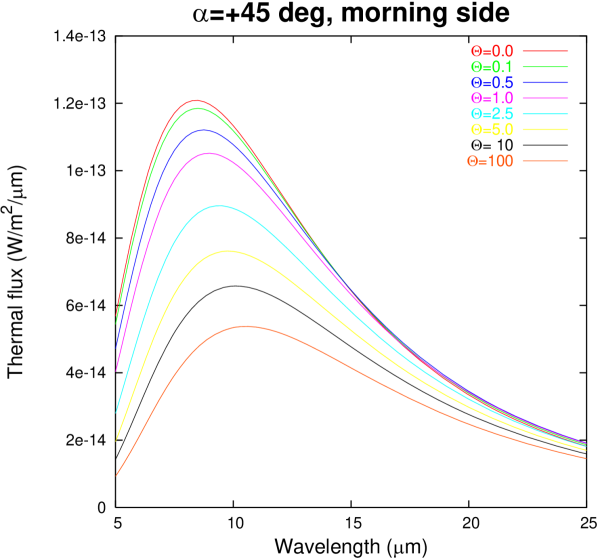
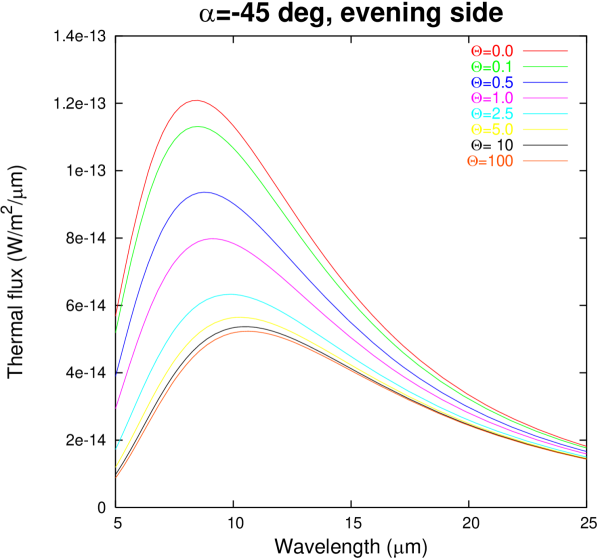
Figure 1: Thermal model spectra of a spherical smooth NEA for different values of $\Theta$, which is proportional to thermal inertia $\Gamma$, and for phase angles of $\alpha=\pm$45\text{\,}\mathrm{\SIUnitSymbolDegree}$$, placing the sub-observer point at local times of 9 AM and 3 PM, respectively (Sun and observer are above the equator). Note the large morning-evening asymmetry for intermediate $\Theta$ values, which asymptotically vanishes for low and large $\Theta$ values. This asymmetry drives the important Yarkovsky effect (see sect. 3) and facilitates determinations of thermal inertia from thermal data despite the competing effect of thermal-infrared beaming which does not display a morning-evening asymmetry. Model parameters are $r=$1.1\text{\,}\text{AU}$$, $\Delta=$0.1\text{\,}\text{AU}$$, $\mathcal{P}=$6\text{\,}\mathrm{h}$$, $A=0.1$, and $\epsilon=0.9$. Hence, $\Theta=1$ corresponds to $\gamma\sim$160\text{\,}\mathrm{J}\usk\power{\mathrm{s}}{-1/2}\power{\mathrm{K}}{-1}\power{\mathrm{m}}{-2}$$. A typical value for NEAs is $300\text{\,}\mathrm{J}\usk\power{\mathrm{s}}{-1/2}\power{\mathrm{K}}{-1}\power{\mathrm{m}}{-2}$ (see sect. LABEL:sect:NEA:TI).

When observing the effect of thermal conduction on asteroid thermal fluxes, the primary observable quantity is $\Theta$ (see eqn. 10c). As can be seen from Fig. 1, $\Theta$ is difficult to measure in the limiting cases when it approaches 0 or $\infty$, and is most readily measurable for intermediate values of the order of 1.

Depending on their angular spin velocity $\omega$ and the subsolar temperature $T_{SS}{}$ (which depends chiefly on the heliocentric distance $r$), objects with identical thermal inertia may nevertheless have very different thermal parameters. While it is intuitively clear that the surface temperatures of fast rotators are more significantly influenced by thermal conduction than those of cold rotators, the dependence of $\Theta$ on $T_{SS}{}$ is less intuitively obvious; to explain the latter, it is instructive to think of thermal emission into space (proportional to $T_{SS}{}^{4}$) as a heat transfer mechanism which competes with conduction into the subsoil (proportional to $T_{SS}{}$). This explains, among other things, why the STM (which assumes $\Theta=0$) appears to be a poor thermal model for Kuiper belt objects (see Stansberry2007, and references therein) despite the low thermal inertia typically expected for such objects: Due to their large heliocentric distances, Kuiper belt objects are cold, and hence $\Theta$ can no longer be neglected even for low $\Gamma$ values.

The three physical parameters $\rho$, $c$, and $\kappa$ cannot be determined separately, but only the thermal inertia $\Gamma=\sqrt{\rho c\kappa}$ (see eqn. 10d). As can be seen from table 1 on p. 1, for plausible asteroid-surface materials $\kappa$ is much more variable than $\rho$ and $c$, hence $\Gamma$ is largely determined from $\kappa$. $\Gamma$ is often transformed into $\kappa$ and vice-versa assuming typical values of $\rho$ and $c$. Confusingly, it is common practice among modelers of the Yarkovsky and YORP effects to consider $\kappa$ as the primary variable (see, e.g., Bottke2006, and references therein; “thermal inertia” is often not mentioned in such papers), while thermal observers and modelers tend to highlight $\Gamma$ rather than $\kappa$.

Geological interpretation

Table 1: Thermal properties of some typical materials: thermal conductivity $\kappa$, mass density $\rho$, specific heat capacity $c$, all for temperatures of $20\text{\,}\mathrm{\SIUnitSymbolCelsius}$ unless otherwise stated. Thermal inertia $\Gamma$ is calculated from eqn. 10d, skin depths $l_{S}$ from eqn. 10a, assuming periods of $\mathcal{P}=$24\text{\,}\mathrm{h}$$ or $365\text{\,}\dday$. References: Text books and standard tables (Dubbel; VolgerLaasch1989; Berber1999; Huette), and WinterKrupp1971 for lunar regolith. Values in parentheses were estimated based on similar materials.

Material	$\kappa$	$\rho$	$c$	$\Gamma$	$l_{S}$ (day)	$l_{S}$ (year)
	W K -1 m -1	k g m	J k g K	J s -1/2 K -1 m -2	c m	c m
Nickel	91	8850	448	$19\cdot 10^{3}$	56	$1000$
Iron	81	7860	452	$17\cdot 10^{3}$	56	$1000$
Granite	2.9	2750	890	2600	13	250
Marble	2.8	2600	800	2400	14	260
Water ice, $0\text{\,}\mathrm{\SIUnitSymbolCelsius}$	2.25	917	2000	2040	13	252
Water, $0\text{\,}\mathrm{\SIUnitSymbolCelsius}$	0.56	1000	4200	1500	4.3	82
Snow (compact)	0.46	560	2100	740	7.3	140
Sandy soil	0.27	1650	800	600	5.3	100
Coal	0.26	1350	1260	665	4.6	88
Pumice	0.15	800	(900)	330	5.4	100
Paper	0.12	700	1200	320	4.4	85
Polystyrene foam	0.03	50	1500	47	7.4	140
Air, $20\text{\,}\mathrm{\SIUnitSymbolCelsius}$	0.026	1.2	1000	5.6	55	1000
Lunar regolith	0.0029	1400	640	51	0.7	13

Note: The entry for air only applies to small volumes of air, where convective heat transfer (which dominates in large volumes) is inefficient. For very porous bodies on Earth (such as polystyrene foam), heat conduction through air trapped inside the pores is the dominant heat transfer mechanism, placing a lower limit on thermal conductivity. On atmosphereless bodies such as the Moon or asteroids, lower conductivities are possible.

As can be seen in table 1 on p. 1, the thermal inertia of lunar regolith is around $50\text{\,}\mathrm{J}\usk\power{\mathrm{s}}{-1/2}\power{\mathrm{K}}{-1}\power{\mathrm{m}}{-2}$, roughly that of very light polystyrene foam. Other plausible soil materials, such as coal or sand, have much larger thermal inertia, and bare rock (granite or marble) reaches , some 50 times larger than that of lunar regolith. Metals are excellent thermal conductors, metallic meteoroids may therefore display a very large thermal inertia some 350 times larger than that of lunar regolith.

The thermal inertia of a given particulate material decreases with decreasing grain size unless grains are much larger than the thermal skin depth (see, e.g., Jakosky1986; Clauser1995; Presley1997). Thermal inertia is thus a very sensitive indicator for the presence or absence of loose surface material. This is widely used in Martian geology (see, e.g., Mellon2000; Christensen2003; Putzig2005, and references therein). It must be noted, however, that even the thin Martian atmosphere greatly enhances the thermal conduction among fine grains (see Presley1997) relative to purely radiative heat transfer. To the best of our knowledge, the dependence of thermal inertia on grain size in a vacuum has not been studied so far, therefore it is presently not straightforward to interpret thermal-inertia values on asteroids in terms of grain size.

Another trend apparent in table 1 is that thermal inertia decreases with porosity (see the difference between ice and snow or the low thermal inertia of volcanic pumice). It is therefore hard to tell a priori what thermal inertia an asteroid composed of “bare rock” should display, but the commonly quoted value of $2,500\text{\,}\mathrm{J}\usk\power{\mathrm{s}}{-1/2}\power{\mathrm{K}}{-1}\power{\mathrm{m}}{-2}$ (see the values for granite and marble in table 1) may be expected to be an upper limit.

It is also apparent from table 1 that neglecting lateral heat conduction on asteroid surfaces is unlikely to introduce significant systematic uncertainties: Even metallic objects with their huge thermal inertia and with a relatively slow rotation rate of $24\text{\,}\mathrm{h}$ would have a thermal skin depth of only $56\text{\,}\mathrm{cm}$, such that for all objects larger than a few tens of meters in diameter lateral heat conduction can be safely neglected. However, lateral heat conduction is very important for thermal modeling of the precursor bodies of metallic meteoroids and their Yarkovsky drifts. Since such objects cannot be observed with current mid-IR telescopes, they are beyond our scope.

Heat transfer mechanisms

There are three major heat transfer mechanisms: conduction, convection, and thermal radiation. While convection is irrelevant on atmosphereless bodies, both conductive and radiative heat transfer could plausibly occur on asteroids. Conduction would be expected to occur within surface grains, while radiation should dominate the heat transfer between grains. In the limit of point-like grains, conduction vanishes while for compact bodies radiative heat transfer can be neglected. The relative importance of the two heat transfer processes thus depends on the typical surface-grain size, which is unknown for asteroids.

For conductive heat transfer, $\kappa$ is largely independent of temperature $T$ (for the materials and the temperature range relevant for our purposes) whereas radiative heat transfer is well described with $\kappa\propto T^{3}$. For lunar regolith, it is known from Apollo in-situ measurements and laboratory analysis of returned lunar samples that both conductive and radiative heat transfer are relevant, such that $\kappa=a+bT^{3}$ with constants $a$ and $b$ (see, e.g., Jones1975, and references therein; in their model, $a$ and $b$ are functions of depth).

Kuehrt1989 proposed a complex TPM in which lunar results are rescaled to the conditions prevailing on the Martian satellites. When attempting to use their model to fit observational data of Deimos and Phobos, however, they reverted to a simplified model, in which only the radiative $T^{3}$ term is considered (Giese1990; Kuehrt1992). Note that in this case heat transfer is no longer described by the diffusion equation eqn. 8 on p. 8, but an additional term occurs, which stems from the derivative of $\kappa$.

Most TPMs for asteroids proposed so far assume $\Gamma$ to be independent of depth and temperature (see Spencer1989; LagerrosI; Delbo2004; Wright2007, and references therein). This implicitly prefers conductive over radiative heat transfer. Another, widely quoted, interpretation is that the exact dependence of thermal parameters on depth and temperature is too poorly constrained by available data to be modeled explicitly, hence one reverts to constant values which are effective averages over the relevant length scales.

Due to their generally lower heliocentric distance, NEAs are typically hotter than MBAs, hence one might expect the radiative $T^{3}$ term to be more important for their thermal emission than for that of MBAs. However, the relative importance of the $T^{3}$ radiative term and the $T^{0}$ conductive term are not clear a priori. An “Apollo-like” thermal conductivity model with two or more fit parameters ($a$ and $b$ given above) would probably be most realistic, but the ratio $a/b$ would be very hard to constrain with typical asteroid data. We adopted a model in which all thermal properties including $\kappa$ are assumed to be constant, but we note that it may be worthwhile to consider a model in which $\kappa$ is proportional to $T^{3}$. This is left to future work.

3 Thermal-infrared beaming

As introduced in sect. 3, the emission characteristics of asteroids surfaces are different to those of smooth Lambertian surfaces, with an observed relative temperature and flux enhancement at low phase angles which, due to conservation of energy, must correspond to relative flux losses at large phase angles. This phenomenon is referred to as thermal-infrared beaming and is well known from thermal observations of the Moon (see, e.g., Saari1972, for an overview) and Mercury (e.g. Emery1998). The surfaces of these bodies are well known to be densely covered with impact craters; “cratered” thermophysical models were seen to reproduce the observed beaming well (see, e.g., Buhl; WinterKrupp1971; Emery1998). In these models, craters are modeled as sections of hemispheres and the beaming effect stems from mutual heating of facets due to reabsorption of scattered and thermally emitted flux inside the crater, and furthermore from shadowing effects which become relevant at large phase angles, both leading to sharp temperature contrasts on small length scales.

Similar crater models have been successfully applied to planetary satellites (e.g. Giese1990; Kuehrt1992) and are frequently employed to model asteroid surface roughness (see Hansen1977; Spencer1990; LagerrosIV; Delbo2004, and references therein).

These models differ in the degree to which multiple scattering inside craters is taken into account: While Hansen1977 neglect multiple scattering altogether but include shadowing and mutual heating due to reabsorption of thermal flux, Spencer1990 additionally considers multiple scattering of sunlight but not of thermal flux (equivalently, $\epsilon=1$ is assumed inside craters); Delbo2004 follows Spencer1990’s approach. The crater model by Kuehrt1989 is virtually identical to Spencer’s but differs in the treatment of thermal conduction inside craters (see below). The model by LagerrosIV is the most complete crater model currently available: Direct and multiply scattered sunlight, shadowing, and reabsorption and multiple scattering of thermal radiation are taken into account. We here present an improvement over the model by LagerrosIV where multiple thermal scattering is fully considered to all orders (see sect. 3 for our improvement to Lagerros’ model).

Several methods have been proposed in the literature to model thermal conduction inside hemispherical craters. LagerrosIV and Delbo2004 explicitly solve the one-dimensional heat conduction problem for each surface tile inside the crater (see above for limitations of the Delbo2004, model) which is, however, computationally very expensive. Although a more complex model had been proposed by Kuehrt1989, the same authors used a simplified variant thereof for fitting observations of the Martian satellites (Giese1990; Kuehrt1992), in which effectively only one subsoil depth is considered—while this satisfactorily reproduces the effect of thermal inertia on the diurnal lightcurve amplitude, it fails to reproduce the phase lag introduced by thermal inertia. We use an approximation proposed and validated by LagerrosIV (see sect. 3) in which the numerical treatment of thermal conduction and cratering decouple, which is numerically highly advantageous.

Model assumptions

Beaming is modeled by adding craters to each surface facet. Variable model parameters are the crater opening angle (equivalent to the relative crater depth) and the crater density, i.e. the surface fraction covered in craters. Very small craters with diameters comparable to or below the thermal skin depth $l_{S}$ (in the c m -range for typical asteroid surfaces, see table 1 on p. 1) do not contribute significantly to the observable beaming because temperature contrasts are reduced by lateral heat conduction. We shall only consider much larger craters, such that lateral heat conduction can be neglected. Under this assumption, thermal fluxes are independent of the crater size distribution for a given opening angle and crater density. One-dimensional heat conduction inside craters is considered in an approximate way, which decouples the treatment of craters from that of thermal conduction. Multiple scattering and reemission of both sunlight and thermal emission are fully taken into account, our approach is an improvement over that by LagerrosIV, the most complete available in the literature so far. So far, the only considered source of input flux is the Sun; for globally non-convex asteroid shapes, where facets may receive additional flux from one another, a generalized model may be required (see sect. LABEL:sect:TPMconcave:beaming on p. LABEL:sect:TPMconcave:beaming).

Two different radiation fields inside the crater are considered, one at optical wavelengths with total energy density $J_{V}(\vec{r})$ and corresponding absorptivity $1-A$ ($A$ denotes the bolometric Bond albedo); and another radiation field $J_{IR}(\vec{r})$ containing thermal radiation (integrated over all thermal wavelengths), with spectrally constant emissivity = absorptivity $\epsilon$ and reflectivity $1-\epsilon$. These two fields are independent from one another, with the exception that absorption of optical energy is a source of thermal energy.

Geometry

Since the crater size distribution is irrelevant, the crater radius is set to unity without loss of generality. The crater shape then solely depends on the opening angle $\gamma$, where low $\gamma$ corresponds to shallow craters and $\gamma=$180\text{\,}\mathrm{\SIUnitSymbolDegree}$$ corresponds to craters shaped as full hemispheres, the deepest craters considered. The slope of surface facets at the crater rim relative to neighboring smooth facets equals $\gamma/2$. Throughout the following, we use the following parametrization of the crater surface

$$\vec{r}=\left(\begin{array}[]{c}\sin\theta\cos\phi\\ \sin\theta\sin\phi\\ -\cos\theta\end{array}\right)$$ (14)

where $\phi$ runs from 0–$2\pi$ and $\theta$ from 0–$\gamma/2$. The crater floor is at depth $-1$, the crater rim at depth $-\cos(\gamma/2)$, hence the total crater depth is $1-\cos(\gamma/2)$. Note that in our notation the value of the opening angle is twice as large as in the notations of Kuehrt1989; Spencer1990; Emery1998; Delbo2004: in their notation, e.g., the full hemisphere has an opening angle of $90\text{\,}\mathrm{\SIUnitSymbolDegree}$ rather than $180\text{\,}\mathrm{\SIUnitSymbolDegree}$. Hansen1977 and LagerrosIV parametrize crater shape in terms of depth over diameter $S^{\prime}$ rather than opening angle $\gamma$; for comparison the following expressions are helpful:

$$S^{\prime}=\frac{1-\cos(\gamma/2)}{2} =\sin^{2}\left(\frac{\gamma}{4}\right)$$ (15a)

$$1-S^{\prime} =\cos^{2}\left(\frac{\gamma}{4}\right).$$ (15b)

The outbound area element $\vec{\text{d}\mathcal{A}}(\vec{r})$ inside the crater is given by

$$\vec{\text{d}\mathcal{A}}\left(\vec{r}\right)=-\sin\theta\ \vec{r}\ \text{d}\theta\ \text{d}\phi,$$ (16)

in particular the outbound unit normal vector $\vec{n}$ equals

$$\vec{n}\left(\vec{r}\right)=-\vec{r}.$$ (17)

We make frequent use of the local directional cosines of the directions towards the Sun, $m_{S}(\vec{r})$, and the observer, $m_{O}(\vec{r})$; and of the cosines of the angular distances of Sun, $\mu_{S}$, and observer, $\mu_{O}$, from local zenith. All these quantities are clipped to be non-negative. Denoting the unit direction-vector towards the Sun or, respectively, the observer as $r_{x}$ (substitute $S$ or $O$ for $x$) and the unit vector in $z$ direction (i.e. local zenith) as $\vec{e_{z}}$, $\mu_{x}$ equals $\vec{r_{x}}\cdot\vec{e_{z}}$ (or 0 if $\vec{r_{x}}$ is below local horizon) and

$$m_{x}\left(\vec{r}\right)=\begin{cases}-\vec{r}\cdot\vec{r_{x}}&\text{if $\vec{r_{x}}$ is visible from $\vec{r}$}\\ 0&\text{otherwise (i.e.\ $\vec{r}$ is eclipsed/occulted)}\end{cases}$$ (18)

$\vec{r_{x}}$ is visible from $\vec{r}$ if $\mu_{x}$ is positive and if the straight line containing $\vec{r}$ with tangent vector $\vec{r_{x}}$ intersects the sphere circumscribing the crater above the crater rim (in addition to the trivial intersection at $\vec{r}$ itself):

$$\vec{r}\cdot\vec{e_{z}}-2\left(\vec{r}\cdot\vec{r_{x}}\right)\left(\vec{r_{x}}\cdot\vec{e_{z}}\right)>-\cos\left(\frac{\gamma}{2}\right).$$ (19)

The vectors $\vec{r_{S}}$ and $\vec{r_{O}}$ in the crater coordinate system can be constructed from scalar products performed in the asteroid-centric coordinate system (scalar products are invariant under rotations) which is computationally advantageous:

$$\vec{r_{S}} =\left(\begin{array}[]{c}\sqrt{1-\mu_{S}{}^{2}}\\ 0\\ \mu_{S}\end{array}\right)$$ (23)

$$\vec{r_{O}} =\left(\begin{array}[]{c}\sqrt{1-\mu_{O}{}^{2}}\cos\phi_{A}\\ \sqrt{1-\mu_{O}{}^{2}}\sqrt{1-\cos^{2}\phi_{A}}\\ \mu_{O}\end{array}\right).$$ (27)

The $\mu_{x}$ can be calculated from the scalar products of $\vec{r_{x}}$ and $\vec{\text{d}\mathcal{A}}$ and

$$\cos\phi_{A}=\frac{\vec{r_{S}}\cdot\vec{r_{O}}-\mu_{S}\mu_{O}}{\sqrt{1-\mu_{S}{}^{2}}{\sqrt{1-\mu_{O}{}^{2}}}}.$$ (28)

(note that this approach fails when thermal conduction inside the crater is explicitly modeled, since then knowledge of $\vec{r_{x}}$ is required as a function of rotational phase).

Another important quantity in the following discussion is the view factor $V_{rr^{\prime}}$ from $\vec{r}$ to $\vec{r^{\prime}}$. It is defined as the fraction of radiative energy per area leaving the facet centered at $\vec{r}$ and directly striking that at $\vec{r^{\prime}}$. Assuming Lambertian emission, the view factor is a purely geometric quantity symmetric in $\vec{r}$ and $\vec{r^{\prime}}$; it equals

$$V_{rr^{\prime}}=\frac{\left(\vec{n}\cdot\left(\vec{r^{\prime}}-\vec{r}\right)\right)\left(\vec{n^{\prime}}\cdot\left(\vec{r}-\vec{r^{\prime}}\right)\right)}{\pi\left|\vec{r}-\vec{r^{\prime}}\right|^{4}}$$ (29)

with the unit outbound surface-normal vectors $\vec{n}$ and $\vec{n^{\prime}}$. In particular, the solid angle under which a facet is visible at another is proportional to the product of its size and the view factor. Inside a sphere, $\vec{n}=-\vec{r}$ (see eqn. 17), hence (using $\vec{r}\cdot\vec{r}=\vec{r^{\prime}}\cdot\vec{r^{\prime}}=1$)

$$V_{rr^{\prime}}=\frac{(\vec{r}\cdot(\vec{r^{\prime}}-\vec{r}))(\vec{r^{\prime}}\cdot(\vec{r}-\vec{r^{\prime}}))}{\pi\left|\vec{r}-\vec{r^{\prime}}\right|^{4}}=\frac{1}{4\pi}.$$ (30)

The fact that the view factor is constant is a peculiarity of the sphere owing to its high symmetry; it will prove to be crucial in the following. In particular, it enables the analytic evaluation of two important surface integrals:

$$\int\limits_{\mathcal{A}}V_{rr^{\prime}}\text{d}\mathcal{A}=\frac{2\pi}{4\pi}\int\limits_{0}^{\gamma/2}\sin\theta\text{d}\theta=\frac{1-\cos(\gamma/2)}{2}=\sin^{2}\left(\frac{\gamma}{4}\right)$$ (31)

and

$$\int\limits_{\mathcal{A}}V_{rr^{\prime}}m_{x}\left(\vec{r}\right)\text{d}\mathcal{A}=\mu_{x}\sin^{2}\left(\frac{\gamma}{4}\right)\cos^{2}\left(\frac{\gamma}{4}\right).$$ (32)

Proof of eqn. 32.

By construction, the integral over the entire crater $\mathcal{A}$ equals the integral over that part $\mathcal{A}^{\prime}$ from which $\vec{r_{x}}$ is not obstructed because $m_{x}(\vec{r})$ vanishes elsewhere. On $\mathcal{A}^{\prime}$, the integral can be written as $\frac{1}{4\pi}\int_{\mathcal{A}^{\prime}}\vec{r_{x}}\cdot\vec{\text{d}\mathcal{A}^{\prime}}$ (see eqn. 17 and 18) which, by virtue of Gauss’ theorem, equals the sum of three contributions:

1. the integral over the crater “cap” $=\frac{2\pi}{4\pi}\mu_{x}\int_{0}^{\sin(\gamma/2)}\rho\text{d}\rho=\mu_{x}/4\sin^{2}(\gamma/2)=\mu_{x}\sin^{2}(\gamma/4)\cos^{2}(\gamma/4)$

2. the vanishing integral over the “terminator,” i.e. the boundary between volume elements that see or do not see $\vec{r_{x}}$. The surface normal vector of that region is perpendicular to $\vec{r_{x}}$ by construction, hence this integral vanishes (if the entire crater sees $\vec{r_{x}}$, this integral vanishes trivially)

3. the volume integral of the (vanishing) divergence of $\vec{r_{x}}$ inside the region circumscribed by the three areas.

∎

Optical flux

A necessary prerequisite to the determination of the temperature distribution inside the crater is a complete knowledge of the radiation field at optical wavelengths $J_{V}(\vec{r})$. Apart from direct insolation, surface elements receive scattered light from other facets, where multiple scattering occurs, i.e. light scattered from one facet to another may be scattered again at the latter.

There are two approaches to model multiple scattering, either by summing up individual scattering orders (which we will do at the end of this section for illustrative purposes) or by self-consistency, i.e. by solving the integral equation

$$J_{V}(\vec{r})=A\left[\frac{S}{r^{2}}m_{S}(\vec{r})+\int\limits_{\mathcal{A}^{\prime}}J_{V}(\vec{r^{\prime}})V_{rr^{\prime}}\text{d}\mathcal{A}^{\prime}\right],$$ (33)

with solar constant $S$ and heliocentric distance $r$ (in AU). Eqn. 33 can be solved analytically for hemispherical craters because the view factor $V_{rr^{\prime}}$ is constant (see eqn. 30), hence the integral in eqn. 33 is independent of $\vec{r}$, i.e. a mere constant $K_{1}$

$$J_{V}(\vec{r}) =A\left[\frac{S}{r^{2}}m_{S}(\vec{r})+K_{1}\right].$$ (34a)

$$K_{1} =\int\limits_{\mathcal{A}^{\prime}}J_{V}(\vec{r^{\prime}})\frac{\text{d}\mathcal{A}^{\prime}}{4\pi}=A\left[\frac{S}{r^{2}}\int\limits_{\mathcal{A}^{\prime}}m_{S}(\vec{r})\frac{\text{d}\mathcal{A}^{\prime}}{4\pi}+K_{1}\int\limits_{\mathcal{A}^{\prime}}\frac{\text{d}\mathcal{A}^{\prime}}{4\pi}\right]$$ (34b)

by reinserting eqn. 33. Using the integrals eqn. 31 and 32:

$$K_{1} =A\left[\frac{S}{r^{2}}\mu_{S}\sin^{2}\left(\frac{\gamma}{4}\right)\cos^{2}\left(\frac{\gamma}{4}\right)+K_{1}\sin^{2}\left(\frac{\gamma}{4}\right)\right]$$ (35a)

$$K_{1} =A\mu_{S}\frac{S}{r^{2}}\frac{\sin^{2}\left(\gamma/4\right)\cos^{2}\left(\gamma/4\right)}{1-A\sin^{2}\left(\gamma/4\right)}$$ (35b)

such that

$$J_{V}(\vec{r})=A\frac{S}{r^{2}}\left[m_{S}\left(\vec{r}\right)+\mu_{S}\frac{\sin^{2}\left(\gamma/4\right)\cos^{2}\left(\gamma/4\right)}{1-A\sin^{2}\left(\gamma/4\right)}\right].$$ (36)

Correction of the Bond albedo

The presence of craters lowers the albedo relative to that of a flat surface patch. Due to the absorption processes associated with multiple scattering, the crater scatters less optical flux outward than a flat surface of equal area would. The corrected Bond albedo $A_{\text{corr}}$ equals $V_{\text{out}}/V_{\text{in}}$ with total in- and outgoing optical flux $V_{\text{in}}$ and $V_{\text{out}}$, respectively. The total solar flux $V_{\text{in}}$ entering through the crater rim equals $\mu_{S}S/r^{2}$ times the projected area of the crater cap $\pi\sin^{2}(\gamma/2)=4\pi\sin^{2}(\gamma/4)\cos^{2}(\gamma/4)$. The total outgoing flux $V_{\text{out}}$ equals $\int_{\mathcal{A}^{\prime}}\int_{\mathcal{A}}J_{V}(\vec{r^{\prime}})V_{rr^{\prime}}\text{d}\mathcal{A}\text{d}\mathcal{A}^{\prime}$, where the integral is performed over the crater interior $\mathcal{A}^{\prime}$ and the crater cap $\mathcal{A}$. By virtue of Gauss’ theorem, one can deform $\mathcal{A}$ into the complement of the sphere circumscribing the crater (i.e. the range $\gamma/2<\theta<\pi$) without changing the result, such that

$$V_{\text{out}} =\int\limits_{0}^{2\pi}\text{d}\phi\int\limits_{\gamma/2}^{\pi}\sin\theta\text{d}\theta K_{1}\qquad\text{(see eqn.\ \ref{eq:beaming:K1a})}$$

$$=2\pi\left(2\cos^{2}\left(\frac{\gamma}{4}\right)\right)A\mu_{S}\frac{S}{R^{2}}\frac{\sin^{2}(\gamma/4)\cos^{2}(\gamma/4)}{1-A\sin^{2}(\gamma/4)}$$

$$=V_{\text{in}}A\frac{1-\sin^{2}(\gamma/4)}{1-A\sin^{2}(\gamma/4)}$$

such that the corrected Bond albedo reads

$$A_{\text{corr}}=A\frac{1-\sin^{2}(\gamma/4)}{1-A\sin^{2}(\gamma/4)}.$$ (37)

Figure 2: Dependence of absorptivity $1-A$, which determines temperatures, on the albedo correction due to the presence of craters (see eqn. 37) as a function of crater opening angle $\gamma$ for different values of flat-surface Bond albedo $A$. To convert $A$ into geometric albedo $p_{\text{V}}{}$, $G=0.15$ is assumed (see sect. 1).

See Fig. 2 for a depiction of the relative changes in absorptivity $1-A$. For realistic asteroid albedos $p_{\text{V}}{}\leq 0.6$ (see sect. 1; $p_{\text{V}}{}=0.6$ corresponds to $A=0.24$ assuming $G=0.15$, see sect. 1), the relative change in absorptivity cannot greatly exceed $10\text{\,}\%$, leading to only moderature changes in temperature since $T\propto\sqrt[4]{1-A}$. It is, however, very important to use the corrected Bond albedo when verifying that the ingoing optical flux equals the total optical and thermal flux, which is an important test of model consistency used in the following.

Direct summation of scattered light to all orders

It is instructive to verify eqn. 36 by explicitly summing up scattered contributions to all orders, which can be performed analytically in this case: For the sake of this discussion, let us denote the amount of directly scattered sunlight emanating from $\vec{r}$ as $J_{0}(\vec{r})$ and the $n$-times scattered component as $J_{n}(\vec{r})$. Then

$$J_{V}(\vec{r})=\sum_{n=0}^{\infty}J_{n}(\vec{r})$$ (38)

and the following relations hold:

$$J_{0}(\vec{r}) =A\frac{S}{r^{2}}m_{S}(\vec{r})$$

$$J_{1}(\vec{r}) =A\int\limits_{\mathcal{A}^{\prime}}J_{0}(\vec{r^{\prime}})V_{rr^{\prime}}\text{d}\mathcal{A}^{\prime}=A^{2}\frac{S}{r^{2}}\mu_{S}\sin^{2}\left(\frac{\gamma}{4}\right)\cos^{2}\left(\frac{\gamma}{4}\right)$$

$$\forall_{n\geq 1}:J_{n+1}(\vec{r}) =A\int\limits_{\mathcal{A}^{\prime}}J_{n}(\vec{r^{\prime}})V_{rr^{\prime}}\text{d}\mathcal{A}^{\prime}=A\sin^{2}\left(\frac{\gamma}{4}\right)J_{n}(\vec{r})$$

(the middle equation holds because of eqn. 32 and, inductively, implies the third equation together with eqn. 31—note that all $J_{n}(\vec{r})$ are independent of $\vec{r}$ for $n\geq 1$). Eqn. 38 acquires the form of a geometric series and can be summed up analytically ($\sum_{n=0}^{\infty}q^{n}=1/(1-q)$ for $|q|<1$; here, $q=A\sin^{2}(\gamma/4)<1$), yielding eqn. 36.

Temperature distribution

Similar to the total optical flux $J_{V}(\vec{r})$, the total thermal flux emanating from $\vec{r}$, $J_{IR}(\vec{r})$, equals the sum of the locally emitted flux $\epsilon\sigma T^{4}(\vec{r})$ plus the flux scattered away from $\vec{r}$

$$J_{IR}(\vec{r}) =\epsilon\sigma T^{4}(\vec{r})+(1-\epsilon)\int\limits_{\mathcal{A}^{\prime}}J_{IR}(\vec{r^{\prime}})V_{rr^{\prime}}\text{d}\mathcal{A}^{\prime}$$ (39)

$$=\epsilon\sigma T^{4}(\vec{r})+(1-\epsilon)K_{2},$$ (40)

where, again, $K_{2}$ is constant because the view factor $V_{rr^{\prime}}$ is constant. As above

$$K_{2} =\int\limits_{\mathcal{A}^{\prime}}J_{IR}\left(\vec{r^{\prime}}\right)V_{rr^{\prime}}\text{d}\mathcal{A}^{\prime}=\epsilon\sigma\int\limits_{\mathcal{A}^{\prime}}T^{4}(\vec{r^{\prime}})\frac{\text{d}\mathcal{A}^{\prime}}{4\pi}+(1-\epsilon)K_{2}\sin^{2}\left(\frac{\gamma}{4}\right)$$

$$K_{2} =\frac{\epsilon\sigma}{1-(1-\epsilon)\sin^{2}(\gamma/4)}\int\limits_{\mathcal{A}^{\prime}}T^{4}(\vec{r^{\prime}})\frac{\text{d}\mathcal{A}^{\prime}}{4\pi}.$$ (41)

Sources of the temperature field $T(\vec{r})$ are absorption of direct sunlight, of scattered optical flux (see eqn. 36), of direct and scattered emission $J_{IR}(\vec{r})$ received from other facets, and thermal conduction from the subsoil:

$$\left(\frac{T(\vec{r})}{T_{SS}{}}\right)^{4} =m_{S}(\vec{r})+\int\limits_{\mathcal{A}^{\prime}}\left[\left(1-A\right)\frac{J_{V}(\vec{r^{\prime}})}{\epsilon\sigma T_{SS}{}^{4}}+\epsilon\frac{J_{IR}(\vec{r^{\prime}})}{\epsilon\sigma T_{SS}{}^{4}}\right]V_{rr^{\prime}}\text{d}\mathcal{A}^{\prime}+\frac{\Theta}{T_{SS}{}}\frac{\partial T}{\partial z}$$ (42)

$$=m_{S}\left(\vec{r}\right)+\frac{1-A}{\epsilon\sigma T_{SS}{}^{4}}K_{1}+\frac{\epsilon}{\epsilon\sigma T_{SS}{}^{4}}K_{2}+\frac{\Theta}{T_{SS}{}}\frac{\partial T}{\partial z}$$ (43)

where the temperature derivative in the last term is with respect to the dimensionless depth coordinate of the one-dimensional heat-conduction problem considered in sect. 2, which is not to be confused with the $z$ coordinate in the crater coordinate system. See eqn. 10b for the definition of the subsolar temperature $T_{SS}{}$.

If thermal inertia is explicitly modeled inside the crater, eqn. 43 takes the role of the surface boundary-condition eqn. 11b of the heat-conduction problem, which must be solved in conjunction with eqn. 41.

If thermal conduction is neglected inside craters, the last term in eqn. 43 vanishes, such that $K_{2}$ can be determined by inserting eqn. 43 and eqn. 35 into eqn. 41:

$$K_{2}=\epsilon\sigma T_{SS}{}^{4}\mu_{S}\frac{\sin^{2}(\gamma/4)}{1-A\sin^{2}(\gamma/4)}\qquad\text{neglecting thermal conduction}$$ (44)

and hence

$$\left(\frac{T\left(\vec{r}\right)}{T_{SS}{}}\right)^{4}=m_{S}(\vec{r})+\frac{\mu_{S}\sin^{2}\left(\gamma/4\right)}{1-A\sin^{2}\left(\gamma/4\right)}\left(\epsilon+A\cos^{2}\frac{\gamma}{4}\right).$$ (45)

This represents an analytic solution to the temperature distribution inside the crater, where multiple scattering of both sunlight and thermal asteroid radiation are taken into account to all orders (LagerrosIV).

Fluxes

The observable thermal flux $F(\lambda)$ at wavelength $\lambda$ is the sum of the directly emitted flux component $F_{0}(\lambda)$ and an infinite number of scattered components $F_{i}(\lambda)$, where the index $i>0$ denotes the scattering order

$$F(\lambda)=\sum_{i=0}^{\infty}F_{i}(\lambda).$$

Each of these components equals an integral of the respective local flux component $F_{i}(\lambda,\vec{r})$ over the visible portion of the crater. In particular

$$F_{0}\left(\lambda\right) =\int\limits_{\mathcal{A}}\frac{m_{O}\left(\vec{r}\right)}{\pi\Delta^{2}}F_{0}\left(\lambda,\vec{r}\right)\text{d}\mathcal{A}$$ (46a)

$$F_{0}\left(\lambda,\vec{r}\right) =\epsilon B\left(\lambda,T\left(\vec{r}\right)\right)$$ (46b)

with the Planck function $B(\lambda,T)$ (see eqn. 6), the observer-centric distance $\Delta$, and the local directional cosine towards the observer $m_{O}$ (see eqn. 18). Scattered orders are determined recursively

$$F_{i+1}\left(\lambda\right) =\int\limits_{\mathcal{A}}\frac{m_{O}\left(\vec{r}\right)}{\pi\Delta^{2}}F_{i+1}\left(\lambda,\vec{r}\right)\text{d}\mathcal{A}$$ (47a)

$$F_{i+1}\left(\lambda,\vec{r}\right) =(1-\epsilon)\int\limits_{\mathcal{A}}F_{i}\left(\lambda,\vec{r}\right)\frac{\text{d}\mathcal{A}}{4\pi},$$ (47b)

where we have used $V_{rr^{\prime}}=1/4\pi$ (eqn. 30). In particular

$$F_{1}\left(\lambda,\vec{r}\right) =(1-\epsilon)\int\limits_{\mathcal{A}}\epsilon B\left(\lambda,T\left(\vec{r}\right)\right)\frac{\text{d}\mathcal{A}}{4\pi}$$ (48a)

$$F_{1}\left(\lambda\right) =(1-\epsilon)\int\limits_{\mathcal{A}}\frac{m_{O}(\vec{r})}{\pi\Delta^{2}}\frac{\text{d}\mathcal{A}}{4\pi}\int\limits_{\mathcal{A}^{\prime}}\epsilon B\left(\lambda,T\left(\vec{r^{\prime}}\right)\right)\text{d}\mathcal{A}^{\prime}$$ (48b)

$$=(1-\epsilon)\mu_{O}\frac{\sin^{2}(\gamma/4)\cos^{2}(\gamma/4)}{\pi\Delta^{2}}\int\limits_{\mathcal{A}}F_{0}\left(\lambda,\vec{r}\right)\text{d}\mathcal{A}.$$ (48c)

Observable flux according to LagerrosIV

In LagerrosIV, the total observable flux is approximated as the sum of directly emitted flux $F_{0}$ and singly scattered flux $F_{1}$ (c.f. LagerrosIV, eqn. 19),

$$F(\lambda)_{\text{Lagerros}} =F_{0}(\lambda)+F_{1}(\lambda)$$ (49a)

$$=\frac{\epsilon}{\pi\Delta^{2}}\int\limits_{\mathcal{A}}\left[m_{O}(\vec{r})+\mu_{O}\sin^{2}\left(\frac{\gamma}{4}\right)\cos^{2}\left(\frac{\gamma}{4}\right)(1-\epsilon)\right]B\left(\lambda,T\left(\vec{r}\right)\right)\text{d}\mathcal{A}.$$ (49b)

It is not discussed therein why higher scattering orders are neglected.

Observable flux to all orders

While, to the best of our knowledge, this has not been discussed in the literature so far, it is feasible to consider all scattering orders in the calculation of observable flux. To this end it is crucial to realize that, because the view factor $V_{rr^{\prime}}=1/4\pi$ is constant, all scattered flux components $F_{i>0}(\lambda,\vec{r})$ are actually independent of $\vec{r}$ as is easily seen in the recursion eqn. 47. Hence

$$F_{i+1}\left(\lambda,\vec{r}\right)=(1-\epsilon)\int\limits_{\mathcal{A}}F_{i}\left(\lambda,\vec{r}\right)\frac{\text{d}\mathcal{A}}{4\pi}=(1-\epsilon)\sin^{2}\left(\frac{\gamma}{4}\right)F_{i}\left(\lambda,\vec{r}\right)$$ (50)

for all $i\geq 1$ (using eqn. 31). The sum of all scattered flux components acquires the form of a geometric series

$$\sum_{i=1}^{\infty}F_{i}\left(\lambda\right)=F_{1}\left(\lambda\right)\sum_{i=0}^{\infty}\left[(1-\epsilon)\sin^{2}\left(\frac{\gamma}{4}\right)\right]^{i}=\frac{F_{1}\left(\lambda\right)}{1-(1-\epsilon)\sin^{2}(\gamma/4)}$$ (51)

and the flux to all orders reads

$$F(\lambda) =\sum_{i=0}^{\infty}F_{i}(\lambda)$$

$$=\frac{\epsilon}{\pi\Delta^{2}}\int\limits_{\mathcal{A}}\left[m_{O}(\vec{r})+\frac{\mu_{O}(1-\epsilon)\sin^{2}(\gamma/4)\cos^{2}(\gamma/4)}{1-(1-\epsilon)\sin^{2}(\gamma/4)}\right]B\left(\lambda,T\left(\vec{r}\right)\right)\text{d}\mathcal{A}.$$ (52)

Note, in particular, that the only difference between this expression and Lagerros’ approximation (eqn. 49) is the redefinition of a constant factor, hence the effort to evaluate them through numerical integration is identical.

The difference between the two expressions is in second and higher scattering orders, i.e. of the order $(1-\epsilon)^{2}$. For asteroids, $\epsilon\sim 0.9$, this would be expected to lead to differences at the percent level, only. This has been verified numerically (see Fig. 3 on p. 3); only for rather unrealistically small $\epsilon$ values do the two expressions differ by more than $10\text{\,}\%$. However, since the effort in numerical evaluation is identical, there is no good reason not to use the full solution.

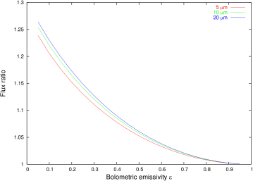
Figure 3: Ratio of crater model fluxes resulting from the solution to all scattering orders eqn. 52 relative to Lagerros’ approximate treatment eqn. 49 as a function of $\epsilon$. Both Sun and observer are at local zenith, used parameters are $\gamma=$180\text{\,}\mathrm{\SIUnitSymbolDegree}$$, $r=$1.1\text{\,}\text{AU}$$, $A=0.1$. Model fluxes were determined using the code described in sect. 3.

Approximative treatment of thermal conduction inside craters

We do not explicitly model thermal conduction inside the crater, but rather use an approximation proposed by LagerrosIV. There, it is proposed that the relative temperature change due to thermal inertia inside the crater equals the relative temperature change outside the crater:

$$\frac{T_{\text{crater}}(\Theta)}{T_{\text{crater}}(0)}=\frac{T_{\text{smooth}}(\Theta)}{T_{\text{smooth}}(0)}.$$ (53)

Under this approximation, the numerical treatment of cratering decouples from that of thermal conduction. In particular, advantage can be taken of the analytic expression for the temperature distribution inside the crater neglecting thermal conduction (eqn. 45).

LagerrosIV generated model fluxes using both his full-blown model and a simplified model making the approximation eqn. 53. He found that the latter systematically overestimates fluxes relative to the former, increasingly so with increasing crater opening angle and thermal parameter, but mutual agreement stayed within $1\text{\,}\%$ for the specific circumstances of his test.

While this is not discussed in LagerrosIV, the approximation eqn. 53 can not be used on the night side, where temperatures would vanish without thermal inertia. We therefore neglect craters on the night side altogether. For the same reason, temperature ratios diverge close to the terminator. Together with the finite spatial resolution of the shape models used by us, this leads to random occurrences of unphysically large flux contributions from facets close to the terminator. To prevent such overshoots, we clip the temperature ratio on the right-hand side of eqn. 53 to be $\leq 1.3$; we have verified that model fluxes are largely independent of the precise value of this threshold value within reasonable limits.

3 Implementation

Our TPM model code has been implemented in C++. It compiles on a Windows XP platform using the compiler which is part of the Visual Studio .NET 2003 suite and furthermore under Linux using gcc. All debugging and testing has been performed under Windows.

In the code development, emphasis was put on a transparent, generic, and object-oriented code structure which makes it easy to add new features. Numerical efficiency was not a primary implementation goal. If in doubt, we erred on the side of simplicity and understandability as opposed to sophistication and obscurity. Not only does this save on development time (including time required for potential further development) but it also helps in the physical validation of the code. On the other hand, the model code is numerically quite inefficient, such that fits to large databases can require several nights of CPU time on a $2.66\text{\,}\mathrm{GHz}$ PC.

1 Class structure

The most important objects inherit from the abstract, generic base classes asteroid or ThermalModelConvex (the latter inherits from the more abstract ThermalModel).

asteroid is a purely abstract base class, only objects belonging to the sub-class TriangulatedConvex can be instantiated. Within its scope, all required information on the asteroid shape and spin state is stored, as well as the constants $H$, $G$, and $\epsilon$. $p_{\text{V}}{}$ is a protected variable within the scope of asteroid, its value can be changed using a routine which also updates the Bond albedo $A$ and the diameter scale factor $s$ (since $H$ is constant, changing $p_{\text{V}}{}$ is equivalent to changing the diameter). TriangulatedConvex contains several routines to calculate disk-integrated thermal fluxes. These routines rely on ThermalModelConvex objects (see below) to calculate flux contributions from single facets; the actual model to be used is specified by passing a reference to the appropriate ThermalModelConvex object. The transformation of heliocentric and observer-centric asteroid coordinates into asteroid-centric directions towards the Sun or the observer (see sect. 1) is performed within the scope of TriangulatedConvex.

The chief interface between asteroid and ThermalModelConvex objects are the functions fluxModFactors and ThermalLightCurveModFactors within the scope of ThermalModelConvex. They return a dimensionless flux value or a dimensionless thermal lightcurve for a given time, observing geometry, and a single facet. All returned flux values must be multiplied by a constant factor of $2\pi\epsilon hc^{2}/(\Delta^{2}\lambda^{5})\times s^{2}$ (with the scale factor $s$ defined in eqn. 2 on p. 2) to convert them into units of W / m ^ 2 / µ m . This multiplication is done by the calling routine within the scope of asteroid after adding contributions from all facets. fluxModFactors is overloaded to allow calculation of fluxes for either a single wavelengths or simultaneously for a vector of wavelengths, the latter significantly increases the efficiency if spectra are calculated for non-vanishing values of thermal inertia.

Important auxiliary classes include ConvexFile, SpinState, and fitFileSI. The latter serves to read in an ASCII file containing thermal flux values along with the epoch and observing geometry of the observations. All model flux values are in units of W / m ^ 2 / µ m . The auxiliary class fitFileMJy is used to read in fit files with fluxes in units of m Jy and to convert them into units of W / m ^ 2 / µ m ; fitFileMJy inherits from fitFileSI.

In order to fit thermal data, the TPM code is used to output ASCII files containing $\chi^{2}$ for different combinations of thermal parameters which are then manually analyzed. Output files are in a suitable format for plotting using the open-source software gnuplot. For each combination of thermal parameters, a best-fit $p_{\text{V}}{}$  is determined analogous to our NEATM-fitting approach (see eqn. 17 on p. 17). If the crater density is considered as a fit parameter, linear regression is used to analytically determine the best-fit crater density. $\chi^{2}$ values are determined by calling an appropriate function at the main-routine level. Prior to this, the data file (or files) are read in and a TriangulatedConvex object is instantiated with all asteroid constants including the shape model (passed as a ConvexFile object) and the SpinState. Then, for each combination of relevant model parameters, a ThermalModelConvex object is instantiated, which is used to calculate model fluxes for the times and observing geometry given in the fit files.

2 Thermal conduction

The subclass of ThermalModelConvex for numerical modeling of thermal conduction on smooth surface elements is ThermalInertiaOnlyConvex. Thermal conduction is modeled as described in sect. 2. The dimensionless heat diffusion equation (eqn. 11) in the subsoil and the boundary condition at the surface (eqn. 11b) are discretized in a straightforward fully explicit way with equidistant sampling points in space and time. This is numerically stable provided the time resolution is not too coarse, specifically (see NR, sect. 19.2) the parameter dTdZ2 (dimensionless time resolution divided by the square of the dimensionless depth resolution) must not exceed 0.5. The numerical integration is truncated at a certain depth, at which the infinite-depth boundary condition eqn. 12 is taken into account.

In the constructor, the thermal parameter and the desired fractional accuracy goal are specified as well as the discretization parameters nTime (number of time steps), nZ (number of depth steps), and zMax (maximum depth in units of skin depths). The constructor checks whether the stability criterion mentioned above is met and throws an exception otherwise.

To calculate surface temperatures, the cosine of the solar angular zenith distance $\mu_{S}$, clipped to be non-negative, is determined for each time step and stored into an array. If all entries are essentially zero, zero flux is returned (the facet is not illuminated for any time of day). Then an array containing the temperature profile is initialized with a constant temperature distribution, and the asteroid is spun until the surface temperature at the desired time has remained constant to within the user-specified fractional accuracy goal. For all time steps, the temperature profile is kept in the computer’s RAM, which proved helpful for debugging and validating the code. An asteroid revolution consists of nTime time steps. For each, the new subsoil temperature profile newP[i] (with $1\leq i\leq\texttt{nZ}-2$) is determined from the old profile oldP[i] using

$$\texttt{newP[i]}=\texttt{oldP[i]}+\texttt{dTdZ2}\left(\texttt{oldP[i-1]}+\texttt{oldP[i+1]}-2\texttt{oldP[i]}\right),$$ (54)

with the parameter dTdZ2 defined above. The surface temperature newP[0] is determined from a discretization of the boundary condition (eqn. 11b)

$$\texttt{newP[0]}^{4}=\mu_{S}+\Theta\frac{\texttt{newP[1]}-\texttt{newP[0]}}{\texttt{dZ}}$$ (55)

with the dimensionless spatial resolution dZ. This nonlinear equation is solved using Newton’s method, with oldP[0] as a first guess for newP[0]. The new temperature at the maximum depth considered, newP[nZ-1], is calculated from eqn. 54 assuming that the fictitious oldP[nZ] equals oldP[nZ-1], thus approximating the boundary condition at infinite depth (eqn. 12)

$$\texttt{newP[nZ-1]}=\texttt{oldP[nZ-1]}+\texttt{dTdZ2}*\left(\texttt{oldP[nZ-2]}-\texttt{oldP[nZ-1]}\right).$$ (56)

Typically used values for nZ, zMax, and nTime are 25, 6, and 300, respectively, a typical value for the fractional accuracy goal is 0.0001.

The fully explicit discretization scheme used to solve the heat diffusion equation and the discretization of the boundary conditions are fully encapsulated within the scope of the class ThermalInertia and its member class TimeStep. Other discretization schemes, such as Crank-Nicholson (see, e.g., NR, sect. 19.2) can be implemented easily without changes to the remaining code.

3 Beaming

Without thermal inertia

Fluxes are calculated by HemisphericNoInertia objects, which inherit from ThermalModelConvex. Returned fluxes are for a crater density of $100\text{\,}\%$ and must be combined with “non-cratered” fluxes in the calling function to account for lower crater densities.

The temperature distribution inside the crater follows from eqn. 45, fluxes are obtained by numerically integrating eqn. 52.

The two-dimensional integral over the crater surface is performed separately for $\phi$ and $\theta$. For each, a Simpson quadrature algorithm has been implemented which adaptively refines the step width until the user-defined fractional accuracy goal is reached (see, e.g., NR, chapt. 4).

Care was taken to minimize the number of calls to the numerically expensive trigonometric functions. E.g., in the polar integral the variable $\theta$ is transformed into $z=\cos\theta$ such that $\int_{0}^{\gamma/2}\sin\theta\text{d}\theta$ becomes $-\int_{\cos\gamma/2}^{1}\text{d}z$.

With thermal inertia

As has been discussed in sect. 3, thermal conduction inside craters is modeled in an approximative way. Model fluxes are calculated by objects belonging to the class InertiaTimesCraterLagerros, which own respectively one instance of HemisphericNoInertia and of ThermalInertiaOnlyConvex.

The ThermalInertiaOnlyConvex object is used to calculate the temperature at a smooth surface patch with thermal conduction. If the Sun is below local horizon ($\mu_{S}\leq 0$), the crater routine is not called, and fluxes are returned corresponding to that temperature. Otherwise, the ratio of the temperature with and without thermal conduction is determined (without thermal inertia, $T/T_{SS}{}=\sqrt[4]{\mu_{S}}$) and clipped to be $\leq 1.3$ (see discussion in sect. 3). “Cratered” model fluxes are calculated with a rescaled temperature distribution. This is accomplished without changes to the implementation of HemisphericNoInertia by using a trick which is based on the fact that fluxModFactors is a function of $\lambda T$, hence rescaling the temperature $T$ is equivalent to rescaling the wavelength $\lambda$ by the same factor (note that the coefficient of the Planck function containing $\lambda^{-5}$ is not multiplied in fluxModFactors but in the calling function). Different fractional accuracy goals can be chosen for the HemisphericNoInertia and ThermalInertiaOnlyConvex objects.

4 Validation

In this section, tests for internal model consistency are reported, with an emphasis on validating the model for application to NEA data, i.e. for large phase angles ($>$30\text{\,}\mathrm{\SIUnitSymbolDegree}$$) and for thermal inertias up to $2500\text{\,}\mathrm{J}\usk\power{\mathrm{s}}{-1/2}\power{\mathrm{K}}{-1}\power{\mathrm{m}}{-2}$. Another important model validation was its application to thermal-infrared observations of a well-studied reference NEA, (433) Eros, which will be reported in sect. 1.

1 Thermal conduction

A first qualitative validation of our thermal-conduction model is from visual inspection of Fig. 2 on p. 2, which was generated using the TPM code. As required, increasing thermal inertia reduces the diurnal temperature contrast and shifts the temperature peak towards the afternoon side. Additionally, the peak temperature at low thermal inertia approaches the theoretical value of $T_{SS}{}$ around $376\text{\,}\mathrm{K}$ (for the parameters specified), while for large thermal inertia the essentially constant temperature approaches $T_{SS}{}/\sqrt[4]{\pi}$ (see sect. 2) or roughly $283\text{\,}\mathrm{K}$ as required.

Due to conservation of energy, the thermally emitted power integrated over one asteroid revolution must match the total absorbed solar power. This was numerically checked, using the discretization parameters stated at the end of sect. 2, a fractional accuracy goal of 0.001, and assuming the situation depicted in Fig. 2—i.e., facet at the equator, $r=$1.1\text{\,}\text{AU}$$, $A=0.1$, $\mathcal{P}=$6\text{\,}\mathrm{h}$$. For a thermal inertia of $10,000\text{\,}\mathrm{J}\usk\power{\mathrm{s}}{-1/2}\power{\mathrm{K}}{-1}\power{\mathrm{m}}{-2}$, the total model emission was found to be too low by roughly $16\text{\,}\%$, around $4\text{\,}\%$ too low for $2500\text{\,}\mathrm{J}\usk\power{\mathrm{s}}{-1/2}\power{\mathrm{K}}{-1}\power{\mathrm{m}}{-2}$, and around $1\text{\,}\%$ for $50\text{\,}\mathrm{J}\usk\power{\mathrm{s}}{-1/2}\power{\mathrm{K}}{-1}\power{\mathrm{m}}{-2}$. Tightening the fractional accuracy goal to 0.0001 incurs a penalty of largely increased program run time, but leads to a conservation of energy to within $1.5\text{\,}\%$ for thermal-inertia values up to $10,000\text{\,}\mathrm{J}\usk\power{\mathrm{s}}{-1/2}\power{\mathrm{K}}{-1}\power{\mathrm{m}}{-2}$, to $0.4\text{\,}\%$ for thermal inertia up to $2,500\text{\,}\mathrm{J}\usk\power{\mathrm{s}}{-1/2}\power{\mathrm{K}}{-1}\power{\mathrm{m}}{-2}$, and much better for lower thermal inertia. No asteroid studied to date displays a thermal inertia larger than $1000\text{\,}\mathrm{J}\usk\power{\mathrm{s}}{-1/2}\power{\mathrm{K}}{-1}\power{\mathrm{m}}{-2}$, hence a fractional accuracy goal of 0.001 is typically sufficient.

We wish to stress that the numerical effort for sufficiently accurate modeling of thermal conduction increases with thermal inertia; TPM codes suitable for MBAs may therefore be unsuitable for NEAs with typically much larger thermal inertia.

2 Beaming without thermal conduction

As detailed in sect. 3, thermal-infrared beaming is an enhancement relative to a Lambertian surface both in absolute flux level and in apparent color temperature for observations taken at low phase angles.

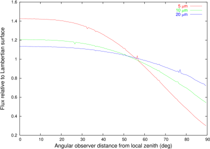
Figure 4: Relative flux enhancement due to a hemispheric crater ($\gamma=$180\text{\,}\mathrm{\SIUnitSymbolDegree}$$) as a function of observer angular distance from local zenith; the Sun is at local zenith. Further model parameters: $r=$1.1\text{\,}\text{AU}$$, $A=0.1$, $\epsilon=0.9$. The slight “wiggles” in the lines are due to numerical noise, they disappear for more stringent accuracy goals (we here use 0.001, a typical value).

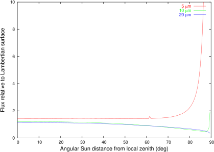
Figure 5: Relative flux enhancement as in Fig. 4, but as a function of solar angular distance from local zenith, with observer at local zenith.

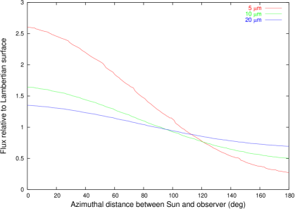
Figure 6: Relative flux enhancement as in Fig. 4 with both Sun and observer placed at a zenith distance of $45\text{\,}\mathrm{\SIUnitSymbolDegree}$, the azimuthal distance between the two is varied.

Figures 4, 5, and 6 show plots of crater fluxes relative to a flat Lambertian surface for hemispherical craters ($\gamma=$180\text{\,}\mathrm{\SIUnitSymbolDegree}$$) and for different viewing geometries (many other opening angles were tested, leading to qualitatively equivalent results). As expected, beaming not only enhances the flux at low phase angles (i.e. low zenith distances in Figures 4 and 5, low azimuthal distance in Fig. 6) but also the apparent color temperature: the flux ratio increases with decreasing wavelength. This is compensated for at large phase angles, when fluxes are reduced relative to a Lambertian emitter—more so at short wavelengths such that the color temperature is reduced relative to a Lambertian emitter.

An important consistency check is to verify the conservation of energy, i.e. to compare ingoing solar flux with the total outgoing energy. For a hemispherical crater of opening angle $\gamma=$180\text{\,}\mathrm{\SIUnitSymbolDegree}$$ and projected area of $\pi$ this means

$$\pi\mu_{S}\left(1-A_{\text{corr}}\right)\frac{S}{r^{2}}=\int\limits_{0}^{\infty}\text{d}\lambda\int\limits_{\mathcal{A}}\text{d}\mathcal{A}\ F(\lambda)$$ (57)

for, e.g., a hemisphere $\mathcal{A}$ above the crater, with the observable flux eqn. 52 and the corrected Bond albedo eqn. 37.

Conservation of energy was tested by numerically integrating eqn. 57 for different values of solar zenith distance (assuming $r=$1.1\text{\,}\text{AU}$$, $A=0.1$, and $\epsilon=0.9$). To this end, the integral over $\text{d}\lambda$ was discretized and truncated with 80 equidistant $\lambda$ steps between 0.5 and $79.5\text{\,}\mathrm{\SIUnitSymbolMicro m}$ using the Simpson integration scheme (see, e.g., NR); for the integral over $\text{d}\mathcal{A}$, a Monte-Carlo scheme was implemented with 2,500 uniformly distributed random directions towards the observer, each Monte-Carlo integration was executed four times with identical parameters in order to gage the statistical noise. The typical scatter among the four runs is $1\text{\,}\%$. In order to gage the absolute accuracy, disk-integrated thermal fluxes were generated for a spherical Lambertian emitter without thermal inertia and integrated those fluxes over $\text{d}\lambda$ and d$\mathcal{A}$. The resulting total thermal power emitted by the asteroid equals the total absorbed power to within the numerical noise ($\sim$1\text{\,}\%$$).

To check the crater routine for conservation of energy, it turned out to be convenient to check it against a Lambertian emitter. To this end, two integrals are calculated using the discretization above, where once the integrand is the output of the crater routine and once that of the Lambertian routine, then the two resulting integrals are compared. Note that the crater induces a reduced albedo $A_{\text{corr}}$ relative to the smooth surface (see sect. 3) due to the increased optical absorption inside the crater. Hence, the “crater integral” should be larger than the Lambertian integral by a factor of $(1-A_{\text{corr}})/(1-A)$, which equals roughly 1.05 for the parameters considered here (see Fig. 2 on p. 2). For a fractional accuracy goal of 0.01, energy was seen to be conserved within $1\text{\,}\%$ (the Sun was placed at zenith distances of 0, 30, and $60\text{\,}\mathrm{\SIUnitSymbolDegree}$).

3 Beaming with thermal conduction

When thermal inertia is considered, ingoing and outgoing radiation are no longer in instantaneous equilibrium but only after integration over a asteroid revolution. The latter integral reduces to a mere sum of contributions from each of the nTime time steps, where for each the integral over $\text{d}\lambda$ and d$\mathcal{A}$ is performed as above. As in the case without thermal inertia, the integral over fluxes returned by an InertiaTimesCraterLagerros object are compared to the integral over Lambertian fluxes multiplied by $(1-A_{\text{corr}})/(1-A)$.

Integration runs were performed for $\mathcal{P}=$6\text{\,}\mathrm{h}$$, and the remaining parameters as in the rest of this section. The Sun was placed at an angular distance of $90\text{\,}\mathrm{\SIUnitSymbolDegree}$ from the spin pole (i.e. over the equator), facets pointing 30, 60, and $90\text{\,}\mathrm{\SIUnitSymbolDegree}$ away from the pole were considered, for thermal-inertia values of 50, 500, and $2500\text{\,}\mathrm{J}\usk\power{\mathrm{s}}{-1/2}\power{\mathrm{K}}{-1}\power{\mathrm{m}}{-2}$. For a fractional accuracy goal of 0.0001 for the treatment of thermal inertia (as in the case of thermal inertia alone) and of 0.01 for cratering (as for cratering alone), energy was found to be conserved to within a few percent in all cases.

5 TPM fits to asteroid data

In principle, our TPM contains four parameters which can be varied independently to obtain the best fit to the data: the diameter $D$ (which is related to $p_{\text{V}}{}$ through the optical magnitude $H$), the thermal inertia $\Gamma$, the crater opening angle $\gamma$, and the crater density $\rho_{c}$. It has been shown by Emery1998 and LagerrosIV that the modeled effect of surface roughness is practically a function of a single parameter, the mean surface slope $\mathrm{bar}{\Theta}$, which is a function of crater opening angle and crater density, reducing the dimensionality of the parameter space by one.

Originally (see Ito1), our approach was to fix the crater opening angle at a constant value and to determine the combination of diameter, thermal inertia, and crater density that best fit the data. In this approach we exploited the fact that, as discussed in sect. 2, model fluxes depend linearly on the assumed crater density. For a given combination of diameter and thermal inertia it is therefore possible to analytically determine the best-fit crater density through linear regression (with the constraint that the density must be non-negative and ).

Later, however, we found that the crater roughness is often not significantly constrained by the data. We find it more instructive and more transparent to use four preset combinations of roughness parameters which span the range of possible surface roughness, and to determine the best-fit diameter and thermal inertia for each. The results are then compared with one another, potentially showing that some roughness model fits the data significantly better than others, and otherwise illustrating the range of roughness-induced uncertainty in thermal inertia and diameter. The four roughness models considered throughout this thesis are

No roughness

$\gamma=0$, $\rho_{c}=0$

Low roughness

$\gamma=$117.70116\text{\,}\mathrm{\SIUnitSymbolDegree}$$, $\rho_{c}=0.4$

Default roughness

$\gamma=$144.59046\text{\,}\mathrm{\SIUnitSymbolDegree}$$, $\rho_{c}=0.6$

High roughness

$\gamma=$151.75834\text{\,}\mathrm{\SIUnitSymbolDegree}$$, $\rho_{c}=1.0$

The parameters for “low”, “default”, and “high” roughness have been defined by Mueller2004 on the basis of thermal-infrared analyses of MBAs.

Synthetic thermal fluxes are generated for the observing geometry and at the wavelengths of the observational data. To fit diameter and thermal inertia for a given set of roughness parameters, model fluxes are calculated on an equidistant grid of thermal-inertia values from the largest value considered down to 0. For each value of thermal inertia, a best-fit diameter is determined from the assumed input diameter and the scale factor $\kappa$ which minimizes

$$\chi^{2}=\sum_{i=1}^{n}\left(\frac{\kappa\cdot m_{i}-d_{i}}{\sigma_{i}}\right)^{2}$$ (58)

(for data points $d_{i}$ with uncertainties $\sigma_{i}$ and synthetic model fluxes $m_{i}$; see eqn. 17). The best-fit diameter and the corresponding $\chi^{2}$ are stored. We neglect that changing the diameter is, for constant $H$, equivalent to changing the albedo, which in principle changes model temperatures and thermal fluxes in a nontrivial way. A full recomputation of model fluxes would, however, be computationally very expensive. We would expect that it is safe to neglect the influence of albedo on temperature if $p_{\text{V}}{}$ is reasonably constant, i.e. if the resulting $\kappa$ value is close to unity (see also sect. 4).

For the first (largest) thermal-inertia value considered in each series, an arbitrary default-value of $p_{\text{V}}{}$ is used. For all following steps, model fluxes are calculated assuming the best-fit $p_{\text{V}}{}$ determined in the previous thermal-inertia step. For not too large steps in thermal inertia, $\kappa$ typically stabilizes to values close to unity within a small number of iterations (see, e.g., sect. 3 for a discussion) such that our approximation above becomes uncritical.

For each roughness model, an ASCII file is output which can be used as a data file for GNUplot. Those files contain, among other things, data lines with entries for thermal inertia, the best-fit $\chi^{2}$ obtained, and the corresponding best-fit $p_{\text{V}}{}$. Best-fit roughness models, thermal inertias, and diameters are then determined from an analysis of the obtained plots (see, e.g., sect. 3). The run time scales with the number of data points and the number of facets in the shape model, typical values range between a few hours and a few days on a $2.66\text{\,}\mathrm{GHz}$ PC.

Chapter 4 Thermal-infrared asteroid observations at the IRTF

The Infrared Telescope Facility (IRTF) is a $3.0\text{\,}\mathrm{m}$ telescope on Mauna Kea / Hawai’i, which is optimized for infrared observations of Solar-System objects. It is operated by the Institute for Astronomy (University of Hawai’i) under a cooperative agreement with NASA. Observing time with the IRTF is made available twice a year in an international open competition.

We have been awarded IRTF time for thermal-infrared observations of asteroids in the semesters 2004A, 2004B, 2005A, and 2005B. Techniques have been established to perform IRTF observations remotely from Berlin. We have used the Mid-InfraRed Spectrometer and Imager (MIRSI) and the optical CCD camera “Apogee,” the latter for support observations. This thesis also contains IRTF thermal-infrared data which have been obtained with the JPL Mid-InfraRed Large-well Imager (MIRLIN). MIRLIN was replaced at the IRTF by MIRSI in 2003.

This chapter contains a brief description of the capabilities of IRTF, MIRSI, and Apogee as needed for our purposes, followed by a section about the remote observing technique established by us (sect. 2). We then explain our observing strategies (sect. 3) and detail the data reduction techniques used by us (sect. 4).

1 IRTF setup and instrumentation

The IRTF is part of the Mauna Kea Observatory / Hawai’i (IAU observatory code 568). Mauna Kea is among the most favorable locations for infrared telescopes worldwide owing to its altitude of some $4200\text{\,}\mathrm{m}$ above sea level, low atmospheric humidity, and good seeing.

The IRTF is a Cassegrain telescope optimized for infrared astronomy. Its primary mirror has an aperture of $3.0\text{\,}\mathrm{m}$. It can be pointed to declinations between $+67\text{\,}\mathrm{\SIUnitSymbolDegree}$ and $-56\text{\,}\mathrm{\SIUnitSymbolDegree}$ at an hour angle within . Differential tracking can be used for for observations of Solar-System objects including NEAs with fast apparent motion.

The Cassegrain secondary mirror provides a $f/35$ beam at the Cassegrain focus where the science instruments are typically situated (an additional Coudé focus is available). IRTF imaging is diffraction limited at mid-infrared wavelengths. The Cassegrain secondary mirror can be oscillated at a frequency up to $40\text{\,}\mathrm{Hz}$ at a maximum projected amplitude of $6\text{\,}\mathrm{\SIUnitSymbolArcminute}$, which is important for, e.g., MIRSI observations (“chopping”; see sect. 1).

Up to four science instruments can be mounted simultaneously at the Cassegrain focus, instrument change-over can normally be accommodated within $30\text{\,}\min$; significantly faster in the case of changes between MIRSI and Apogee, which require only a filter to be moved and require only a few seconds.

The telescope shutter consists of two parts for airmass ranges of up to 1.5 (maximum zenith distance , only one shutter part open) or up to 2.9 (both parts open) (see eqn. 1 on p. 1 for a definition of airmass).

Telescope pointing and tracking is done by the Telescope Operator (TO) who also sets up the instruments. Focusing and fine tuning of the pointing is in the responsibility of the observer; the IRTF software tcs1_status is used for this purpose (see Fig. 1).

Figure 1: tcs1_status, the IRTF tool for focusing and fine tuning of pointing (screenshot from a DLR machine during an IRTF observing run on 27 Sept. 2004).

1 MIRSI

The Mid-Infrared Spectrometer and Imager MIRSI is a mid-infrared camera with imaging capabilities between $\sim 5$ and $26\text{\,}\mathrm{\SIUnitSymbolMicro m}$ and additional spectroscopic capabilities over the 8–14 and $17--26\text{\,}\mathrm{\SIUnitSymbolMicro m}$ atmospheric windows. MIRSI has been built at the Boston University (MIRSI) and has been commissioned at the IRTF in 2003, replacing MIRLIN. It is not an IRTF facility instrument but has been made available by the instrument PI (the late L. Deutsch; now J. Hora) on a collaborative basis. The MIRSI detector is operated at a temperature between $6--12\text{\,}\mathrm{K}$ inside a helium cooled dewar. The MIRSI control computer system is connected to the IRTF mirror control unit such that it can control chop and nod movements (see below).

Table 1: Overview of MIRSI filters used in our programs, together with their estimated $1\sigma$ point-source sensitivity in $1\text{\,}\mathrm{min}$ on-source integration time if mounted on the IRTF (source: MIRSI, for the filter specifications and http://cfa-www.harvard.edu/mirsi/mirsi_spec.html for the sensitivities).

Central wavelength	Width	$1\sigma$ sensitivity for $1\text{\,}\mathrm{min}$ integration
( µ m )	(%)	( m Jy)
4.9	21	16.2
7.8	9.0	46.3
8.7	8.9	59.1
9.8	9.4	19.7
11.7	9.9	24.0
12.3	9.6	(no value given)
18.4	8.0	57.3
24.8	7.9	(no value given)

Our programs make use of MIRSI in imaging mode, the spectroscopy mode is disregarded in the following. The Si:As impurity-band-conduction detector has $320\times 240$ pixels at a projected pixel scale of $0.27\text{\,}\mathrm{\SIUnitSymbolArcsecond}$ when mounted on the IRTF, corresponding to a field-of-view (FOV) size around $$85\text{\,}\mathrm{\SIUnitSymbolArcsecond}$\times$64\text{\,}\mathrm{\SIUnitSymbolArcsecond}$$. At MIRSI wavelengths, IRTF imaging is diffraction limited. See table 1 for a list of MIRSI filters used in our observations.

Due to the high level of background radiation, single MIRSI exposures (frames) typically saturate within fractions of a second, depending on the filter and on atmospheric conditions. MIRSI observations therefore consist of long series of frames, where the desired frame time and total on-source integration time are set by the observer. Depending on the observing mode, observations are taken at different positions to enable correction for background radiation. For our observations, MIRSI was used in chop/nod mode. In chop/node mode, MIRSI commands the telescope’s Cassegrain secondary mirror to “chop”, i.e. to oscillate in a square wave pattern of a user-defined frequency and amplitude ($4\text{\,}\mathrm{Hz}$ and $20\text{\,}\mathrm{\SIUnitSymbolArcsecond}$, in our case). At each chop position, an integer number of frames is taken. Half of the total integration time is chopped at the specified location, then the primary mirror is slewed (“nodded”) to an offset position where a second chop set is taken. Combining chopping and nodding enables more accurate subtraction of background radiation (see, e.g., Delbo2004, sect. 3.3, for a detailed discussion). The data obtained in a chop/nod exposure are stored as a single FITS file with three extensions where each of the four contained images is the sum of all frames taken at one particular beam position.

The directions and amplitudes of the chop and nod movements are set by the TO upon the observer’s request. Timing parameters are specified by the observer through the MIRSI control software.

Due to overheads for, e.g., detector read-out or wait times for the secondary mirror to settle after a chop movement, there is a significant difference between the integration time (i.e. the total time spent collecting measured photons) and the image acquisition time (integration time plus all overheads). All other parameters kept constant, shortening the frame time increases the ratio of acquisition time over integration time.

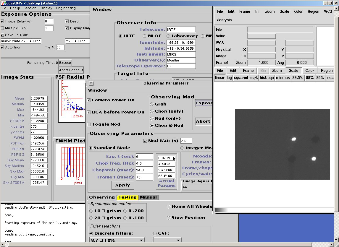
Figure 2: Screenshot of the MIRSI control software during a remote IRTF observing run on 27 Sept. 2004.

In the windows opened by the MIRSI control software (see Fig. 2, see also http://www.cfa.harvard.edu/mirsi/MIRSI_Obs_Guide.pdf for a user guide), the observer specifies the observing mode and corresponding timing parameters, and controls the filter wheel. Information about the target can be entered; this is used by the software to store the target name and the airmass in the header of the resulting FITS file (in addition to the filter used, observation time and duration, etc.). Note that the airmass is not taken directly from the telescope control system (such as that displayed in tcs1_status; see Fig. 1) but is rather calculated from the system date, the telescope coordinates, and the target RA and dec. entered in the target information form—for the latter, it is important to strictly keep the format described in the observer guide because otherwise the program will crash, typically requiring a lengthy reboot of the control computer and instrument re-initialization.

2 Apogee

Apogee is an optical-wavelength camera using a commercial $1024\times 1024$ pixel CCD with a field of view of $66\text{\,}\mathrm{\SIUnitSymbolArcsecond}$. Several filters are available, we used a standard V filter in all our observations. Apogee is thermoelectrically cooled to an operational temperature of to reduce the noise level. We typically used Apogee in $4\times 4$–binning mode (thus shrinking the FOV to $256\times 256$ pixels) to reduce the required detector readout times. Changeover between MIRSI and Apogee or vice-versa takes only a few seconds, enabling nearly-simultaneous optical photometry of MIRSI targets to be obtained.

Apogee is significantly more sensitive to asteroid flux than MIRSI. Using the V filter, signal-to-noise ratios exceeding 100 are reached within a few tens of seconds for all asteroid targets which are sufficiently bright for MIRSI observations.

The Apogee control software automatically saves all obtained data in FITS format.

2 Remote control of observations

The IRTF supports remote control of observations using MIRSI and Apogee. We have established techniques to remotely control IRTF observations from DLR Berlin and have successfully observed remotely a number of times.

During remote observations, the control programs for both MIRSI and Apogee are executed locally at the IRTF, but the screen output and input from mouse and keyboard can be transferred to/from any computer with access to the internet. For this purpose the VNC protocol is used, which is encrypted and password-protected. A VNC viewer program is required to run on the observer’s machine. MIRSI and Apogee require one virtual VNC desktop each. Additionally, observers require access to the program tcs1_status for focusing and pointing fine-tuning. It is advisable to run tcs1_status on another computer within the Institute for Astronomy network. To remotely connect to the machine running tcs1_status from a Windows machine in Berlin, it is most convenient to open a third VNC server on the Hawai’i machine running tcs1_status.

Each VNC server on a machine is identified with its desktop number, which are counted upward starting with 1 (desktop 0 is the native desktop which cannot usually be forwarded). VNC communication between two computers is performed through designated ports, where the default port for a virtual desktop with number $n$ is $5900+n$. Remote control of IRTF observations thus requires the ports 5901, 5902, and 5903 by default. These ports are blocked by the DLR firewall, and the DLR IT administration is reluctant to open them. Instead, these ports were “tunneled” using an encrypted SSH connection.

In addition to the VNC connections, a channel for direct communication with the telescope operator is required. The IRTF default for remote observers is a PolyCom system or, alternatively, a PC running NetMeeting. Since neither possibility was easily feasible from within the DLR network (and because telephone contact over several hours of observing time would have been rather expensive and inconvenient), we proposed an alternative solution which is now among the default options offered by the IRTF, namely voice-over-IP communication.

The Mauna Kea Weather Center (http://hokukea.soest.hawaii.edu/index.cgi) holds many useful resources to remotely check the atmospheric conditions above Mauna Kea. Astronomy-minded weather forecasts for the summit are available (which generally differ vastly from forecasts for the rest of the island) in addition to real-time webcam images from several telescopes at Mauna Kea, real-time meteograms from several telescopes, and nearly-real-time satellite imagery. A particularly useful tool is the CFHT “skyprobe” (http://www.cfht.hawaii.edu/Instruments/Skyprobe/) for estimates of the atmospheric extinction. Significant changes in the extinction typically indicate the presence of clouds. After each observing run, we typically save a copy of the skyprobe plot for the respective night, in addition to a Mauna-Kea meteogram, in order to enable later assessment of the atmospheric conditions.

3 IRTF observing strategy

Figure 3: Coadded and subtracted MIRSI image with the four beams not quite at the nominal position. Note the artefact pattern in the left half of the detector. (Observation of Itokawa, 10 July 2004, 12:53 UT—this frame could not be used to measure the target flux, see table 2 on p. 2)

General considerations

All MIRSI observations are performed in chop/nod mode to enable subtraction of the celestial background. Since our targets are not spatially resolved, the directions of the chop and nod throws are uncritical; we used $20\text{\,}\mathrm{\SIUnitSymbolArcsecond}$ East-West and North-South, respectively. We used a chop frequency of $4\text{\,}\mathrm{Hz}$, a chop wait time of $24\text{\,}\mathrm{ms}$, and a nod wait time of $2\text{\,}\mathrm{s}$.

No flatfield for MIRSI is available and it would be very time consuming to obtain one; to minimize the possible effect of pixel-to-pixel variations in detector sensitivity, we have aimed at keeping all sources at a constant position on the chip using tcs1_status. We chose a nominal position such that the center of the four beam positions is centered in the detector’s $y$ coordinate and at $75\text{\,}\%$ in the $x$ direction, where the latter is motivated by the fact that the detector’s “left” half is occasionally malfunctioning (see Fig. 3 on p. 3). The FOV is large enough to have all four beam positions on the chip, nevertheless.

Apogee observations are interspersed between the MIRSI observations. As for MIRSI, no flatfield is available for Apogee. The telescope is not moved between MIRSI and Apogee observations, such that also for Apogee the on-chip target position is reasonably constant, minimizing the possible effect of pixel-to-pixel variations in sensitivity. Apogee is used with a standard V filter in all our observations.

Calibration observations and observation planning

To facilitate the derivation of absolutely calibrated infrared fluxes and optical V-magnitudes, suitable calibration standard stars are chosen from the lists of CohenVII; CohenX and Landolt1973; Landolt1992 for each observing run. Calibration standards are typically observed at the beginning and at the end of each observing run. If the atmospheric conditions appear slightly unstable, further calibration observations are interspersed between the target observations to gage the atmospheric stability. To facilitate accurate correction for atmospheric extinction (also called airmass correction, see eqn. 2 on p. 2), calibration standards are typically observed at airmasses which bracket those of the primary scientific targets. If the target airmasses span a large range, a calibrator at an intermediate airmass is observed to gage the quality of the airmass correction. Whenever possible, the same calibration standard star is used for all required airmasses (i.e. it is reobserved at a later time) to minimize any possible cross-calibration problems.

The observations are planned such that the science targets are observed at the minimum possible airmass. We furthermore aim at minimizing the number of required changes to the telescope shutter (see sect. 1) which occur when the telescope pointing transgresses an airmass boundary value of 1.5.

Starting an observing run

After starting and initializing all required control units for the telescope itself and the instruments, and, in the case of remote observations, after establishing all required communication channels, the instruments must be initialized (most of these tasks are performed by the TO but may require observer input).

As soon as the instruments are initialized, the telescope should be slewed to a bright MIRSI target, typically a calibration standard star, to focus the telescope using tcs1_status (see Fig. 1 on p. 1). Telescope focus is a function of local temperature, therefore it is required to check occasionally during an observation run whether the telescope is still focused, particularly in the first half of the night when the telescope dome cools down significantly.

At the same time, suitable frame times have to be determined for each MIRSI filter to be used during the night: Frame times are limited by the requirement that the sky background, which vastly dominates the flux at MIRSI wavelengths, must not bring the detector close to saturation, so that the detector response to the source flux remains linear. On the other hand, frame times should be as long as possible to optimize the time efficiency of MIRSI observations (see sect. 1). Background levels can vary greatly on a night-to-night basis, so the optimum frame time must be determined for each MIRSI filter and each observing run. The MIRSI software analyses observational data “on the fly” and displays, among other things, the average, median, and maximum value of sky background radiation (see Fig. 2 on p. 2). Frame times should be chosen which bring the average sky level to values not greatly exceeding 20,000 as displayed by the MIRSI control software (Bus, 2004, private communication). Once determined, the filter-dependent frame times should be used throughout the observing run. Significant changes in the sky background during the night typically indicate non-photometric conditions, with the exception that sky levels grow moderately with airmass and furthermore during twilight.

As soon as Apogee has reached its operational temperature of , we take a number of bias frames. Dark frames are not usually taken. During the first Apogee observations it is verified that Apogee is on focus, otherwise the TO is asked to adjust the relative focus between MIRSI and Apogee.

During the observations

When observing a faint science target, it is usually first observed through the $11.6\text{\,}\mathrm{\SIUnitSymbolMicro m}$ filter which, among MIRSI’s filters, is most sensitive to asteroid thermal emission. From the asteroid brightness in this filter it is estimated how long observations in other filters might take and whether challenging filters, such as the Q-band $18.4\text{\,}\mathrm{\SIUnitSymbolMicro m}$ filter, are tried at all.

During longer observations of a single target, we typically monitor its thermal lightcurve in the $11.6\text{\,}\mathrm{\SIUnitSymbolMicro m}$ filter and intersperse observations in other MIRSI filters and Apogee V-band observations. It is particularly convenient to perform a quick Apogee observation while MIRSI is busy changing filters, which may take up to a minute. For asteroid targets sufficiently bright to be observed with MIRSI, required Apogee integration times with the V filter are of the order of tens of seconds at most, while instrument changeover between Apogee and MIRSI is done within seconds.

During observations, all observation parameters are logged using the log sheets contained at the end of the MIRSI observer guide. Most importantly, the observing time, duration, target name, filter, and airmass are logged in the designated columns. The “comments” column is used, among other things, for logging manual telescope offsets and changes to focus settings.

4 Data reduction

The measured asteroid flux is proportional to the detector response per integration time, the proportionality constant is determined from observations of calibration standard stars. The detector response to exposures is determined through synthetic aperture photometry after instrument-specific image-cleaning procedures.

Measured flux values must be corrected for the effect of atmospheric extinction (“airmass correction”). Corrections for the effect of finite filter breadth (“color correction”) are discussed.

1 MIRSI

MIRSI data reduction is aided by a set of IDL routines developed by Eric Volquardsen, available on-line at http://irtfweb.ifa.hawaii.edu/~elv and described at http://irtfweb.ifa.hawaii.edu/~elv/mirsi_steps.txt. We use the routine mirsi_coad to remove instrument-specific artefacts and to coadd the observations taken at the four chop/nod beam positions with the appropriate signs. Note that cosmic ray hits are not a source of concern for MIRSI observations because their effect is dwarfed by the celestial background.

After coadding, MIRSI images display the source four times with two positive and two negative detections (see, e.g., Fig. 3 on p. 3). These four detections are copied pixel-wise into a single, “registered” detection after determining four non-overlapping regions centered on each of the four detections and inverting the sign of the regions surrounding the negative detections. The edge length of these regions was chosen large enough to facilitate accurate background subtraction during synthetic aperture photometry, while guaranteeing that the region does not exceed the chip boundary. We typically use an edge length of 50 MIRSI pixels corresponding to $13.5\text{\,}\mathrm{\SIUnitSymbolArcsecond}$.

Synthetic aperture photometry

Detector counts are determined by performing synthetic aperture photometry on the registered images. To this end, the pixel content of a synthetic aperture, i.e. a circular region surrounding the source centroid, is added up and corrected for the amount of background radiation contained inside the synthetic aperture. The background level is usually estimated from the pixel content of an annular region centered at the detection centroid. The background annulus should be far enough from the source to be uncontaminated with source flux but should be close enough to provide a good estimate of the local background level (which may be spatially variable). Accurate flux estimation from faint detections (low $S/N$) depends critically on appropriate background estimates. A practical criterion for the appropriateness of a background estimate is whether or not it leads to a stable photometric growthcurve (Howell1989)—see also the detailed discussion in Delbo2004.

Image registration and synthetic aperture photometry on MIRSI images can be automatized using the IDL routines by E. Volquardsen. We felt it was safer to perform these steps interactively, using the IDL-based registration and aperture-photometry tool by M. Delbo2004 which is a modified version of the ATV package by Aaron Barth (http://www.astro.caltech.edu/~barth/atv/). Image registration is done manually as described above. The synthetic aperture photometry routine automatically determines the centroid of the registered source. Care was taken to determine appropriate background values for each source by studying the photometric growthcurve. To avoid systematic uncertainties, the same aperture radius was chosen for all observations obtained during one observing run in a specific filter. To accommodate for possible temporal variations in the width of the point spread function, which may arise due to changes in seeing but also due to focus drifts, conservatively large aperture radii were chosen.

Airmass correction

Fluxes determined from ground-based astronomical observations must be corrected for the effect of atmospheric extinction, which reduces the amount of flux received at the ground. Atmospheric extinction scales with the angular zenith distance of the observed target $\zeta$, most conveniently expressed in terms of the airmass AM

$$\text{AM}:=\frac{1}{\cos\zeta}.$$ (1)

To first order in airmass, the received fluxes $f$ of a constant source observed at different airmasses are related by

$$-2.5\log\frac{f(\text{AM}_{1})}{f(\text{AM}_{2})}=E\left(\text{AM}_{1}-\text{AM}_{2}\right)$$ (2)

with the extinction coefficient $E$ in units of mag/airmass. Extinction coefficients for the Mauna Kea site depend greatly on the wavelength considered and may furthermore vary significantly from night to night (see, e.g., Krisciunas1987, and references therein); at infrared wavelengths, extinction coefficients depend chiefly on the atmospheric water content. A night during which extinction coefficients vary significantly is non-photometric by definition.

Practically, we determine extinction coefficients for each MIRSI filter and observing run by comparing the background-corrected detector response to observations of calibration standard stars at different wavelengths. While it is possible to relate observations of different calibration standard stars in this way, we tried to reobserve the same calibration standard whenever possible, in an attempt to minimize systematic uncertainties in the airmass correction (see sect. 3). Thus determined extinction coefficients were compared to the list compiled by Krisciunas1987 for the Mauna-Kea site, which serves as a useful cross-check.

Once the extinction coefficients are determined, all background-corrected detector counts are referred to the same airmass, where we typically use $\text{AM}=1$. Larger values were occasionally chosen for observations which were obtained at large airmass.

Flux calibration

After correction for background and airmass, detector counts $C$ are proportional to the measured source flux $f$ and the total on-source integration time $t$. Denoting quantities referring to the asteroid target with subscript $a$ and quantities referring to the calibration star with subscript $s$:

$$f_{a}=\frac{C_{a}}{t_{a}}f_{s}\frac{t_{s}}{C_{s}}.$$ (3)

Flux values for calibration stars were taken from CohenVII; CohenX.

Color correction

As can be seen in table 1 on p. 1, MIRSI together with the filters used by us is a broad-band photometer, hence it would be expected that fluxes must be color corrected taking account of the target spectrum and the total spectral response of the combined telescope–filter–detector system (see sect. 4 for a general discussion).

Determination of color-correction factors is here hampered by the lack of published filter transmission curves. Assuming a rectangular transmission curve centered at the central wavelength and with the spectral breadths given in table 1, Delbo2004 determined color-correction factors for all MIRSI filters used by us and a number of black-body temperatures; the accuracy of his results is hard to estimate lacking information on the filter profile. For black-body temperatures between $200and400\text{\,}\mathrm{K}$, which are appropriate for NEAs and MBAs, the thus determined approximate color-correction factors do not exceed a few percent, much below the remaining systematic and statistical uncertainties. Color corrections were therefore not applied to MIRSI fluxes.

2 Apogee

Like for MIRSI, the IRTF provides a set of IDL routines for the reduction of Apogee data developed by Eric Volquardsen (see http://irtfweb.ifa.hawaii.edu/~elv and http://irtfweb.ifa.hawaii.edu/~elv/apogee_steps.txt). The automatized data reduction steps include correction for bias and dark current, detection and removal of cosmic ray hits, synthetic aperture photometry, and airmass correction. We have carefully checked all pipeline elements (e.g. against our independent synthetic aperture photometry routine) and found them to work reliably for our high-signal-to-noise Apogee data. Only the detection and removal of cosmic ray hits requires visual inspection on a case-by-case basis to avoid flagging and “cleaning” parts of the source. The final product of the Apogee data reduction pipeline is an ASCII file containing instrumental magnitudes for all observations. Source magnitudes are determined by adding a constant magnitude offset determined from the instrumental magnitudes of the calibration standards (with V magnitudes listed in Landolt1973; Landolt1992). By default, Volquardsen’s IDL routines determine magnitudes of the brightest source in the field. Occasionally, Apogee’s field of view contained field stars which were brighter (in the V band) than the asteroid target. In resulting image frames, the field star was masked semi-automatically prior to the proper data reduction, for which purpose we have developed an IDL routine.

Chapter 5 Asteroid observations using the Spitzer Space Telescope

The Spitzer Space Telescope (known as Space InfraRed Telescope Facility, SIRTF, until after launch) is the fourth and final member of NASA’s series of space telescopes called Great Observatories, following the Hubble Space Telescope, the Compton Gamma Ray Observatory, and the Chandra X-Ray Observatory. Spitzer has imaging and spectroscopy capabilities in the mid-infrared wavelength range from 3.6–$160\text{\,}\mathrm{\SIUnitSymbolMicro m}$. Spitzer is the currently most sensitive mid-infrared telescope, owing mostly to its vantage point far away from the Earth atmosphere and thermal environment.

Spitzer was launched in 2003 and is expected to stay fully operational until spring 2009. Observing time with Spitzer is made available annually since summer 2004 through an international competition. We were awarded a total of four asteroid observing programs in open competition, two in cycle II (2005–06) and further two in cycle III (2006–07). As of 20 April 2006, i.e. up to Spitzer cycle III, there is a total of 16 asteroid observing programs with Spitzer, including our four.

In sect. 1, some general information on Spitzer is provided, including its optical design. Sections 2 and 3 are devoted to the two focal plane instruments used in our observing programs, the InfraRed Array Camera (IRAC) and the InfraRed Spectrometer (IRS), respectively. In either section, the instrument capabilities are presented and our observing strategies and data reduction techniques are detailed. The scientific goals and achievements of our observations will be discussed in the following chapters.

More information can be found in the Spitzer Space Telescope Observer’s Manual (referred to as SOM in the following) provided on-line by the Spitzer Science Center: http://ssc.spitzer.caltech.edu/documents/som/. See also SST.

1 Spitzer overview

The Spitzer spacecraft carries a $0.85\text{\,}\mathrm{m}$ reflecting telescope with three focal plane science instruments performing imaging and spectroscopy in the wavelength range from 3.6–$160\text{\,}\mathrm{\SIUnitSymbolMicro m}$. In flight, telescope and focal plane instruments are cryogenically cooled with liquid helium. The spacecraft was launched on a Delta rocket from Cape Canaveral, USA on 25 Aug 2003. Its orbit is heliocentric, trailing behind Earth, thus avoiding the adverse affects of the Earth atmosphere and thermal environment. After cooling down the telescope, followed by initial validation and calibration measurements, science observations began on 1 Dec 2003; they are expected to last as long as cryogen is available, probably until spring 2009.

Figure 1: Aperture positions of the Spitzer science instruments on the focal plane. There are several apertures per instrument, corresponding to different instrument operation modes. Those for IRAC will be discussed in sect. 2, those for IRS in sect. 3 (MIPS is not used in our observations). Also on the focal plane are pointing control reference sensors (PCRS). The projected focal plane radius is $16\text{\,}\mathrm{\SIUnitSymbolArcminute}$. (Fig. from SOM, p. 60).

The three science instruments are (see Fig. 1 for their position on the focal plane):

• InfraRed Array Camera (IRAC), four imaging detectors operating at central wavelengths of 3.6, 4.5, 5.8, and $8.0\text{\,}\mathrm{\SIUnitSymbolMicro m}$, respectively, each with a square field-of-view of about $5\text{\,}\mathrm{\SIUnitSymbolArcminute}$ at a pixel scale of (PI G.G. Fazio, Smithsonian Astrophysical Observatory, Harvard-Smithsonian Center for Astrophysics);

• InfraRed Spectrograph (IRS), a spectrometer covering the wavelength range from 5.2–$38.0\text{\,}\mathrm{\SIUnitSymbolMicro m}$ at relative spectral resolutions $\lambda/\Delta\lambda$ between 64 and 128 (low-resolution mode) or $600$ (high-resolution mode). IRS also has imaging capabilities at wavelengths of about 16 and $22\text{\,}\mathrm{\SIUnitSymbolMicro m}$ with a field of view of about $$1\text{\,}\mathrm{\SIUnitSymbolArcminute}$\times$1.2\text{\,}\mathrm{\SIUnitSymbolArcminute}$$ at a pixel scale of (PI J.R. Houck, Cornell University);

• Multiband Imaging Photometer for Spitzer (MIPS), an imager with three broad-band filters centered at wavelengths of 24, 70, and $160\text{\,}\mathrm{\SIUnitSymbolMicro m}$. MIPS has an additional low-resolution ($\lambda/\Delta\lambda\sim 20$) spectroscopy mode at wavelengths of 55–$95\text{\,}\mathrm{\SIUnitSymbolMicro m}$ and a Total Power Mode for measuring the absolute sky brightness in that wavelength range (PI G. Rieke, Steward Observatory, University of Arizona). MIPS is not used in our observing programs and is thus disregarded in the following.

The spacecraft is operated by the Spitzer Science Center (SSC), located at the campus of the California Institute of Technology in Pasadena, CA, USA.

1 Spacecraft design and orbit

Figure 2: Design of the Spitzer spacecraft; it is tall and in diameter. The longest axis coincides with telescope boresight. (Fig. from SOM, p. 35).

See Fig. 2 on p. 2 for an overview of the spacecraft design. Its main components are:

• Cryogenic Telescope Assembly: A cryostat attached to the helium tank; it contains the cold parts of the focal plane science instruments at a helium bath temperature of $1.4\text{\,}\mathrm{K}$. The telescope itself is cooled through helium vapor vented off the cryostat to a temperature of 6–$12\text{\,}\mathrm{K}$.

• Spacecraft Bus, hosting all command and data handling units, along with the systems for attitude control and telecommunication. The spacecraft bus is not cooled, and thermally shielded from the cryogenic telescope assembly.

• Solar Panel and Solar Panel Shield, which provide electric power and at the same time shield the spacecraft (particularly the cryogenic assembly) from direct sunlight.

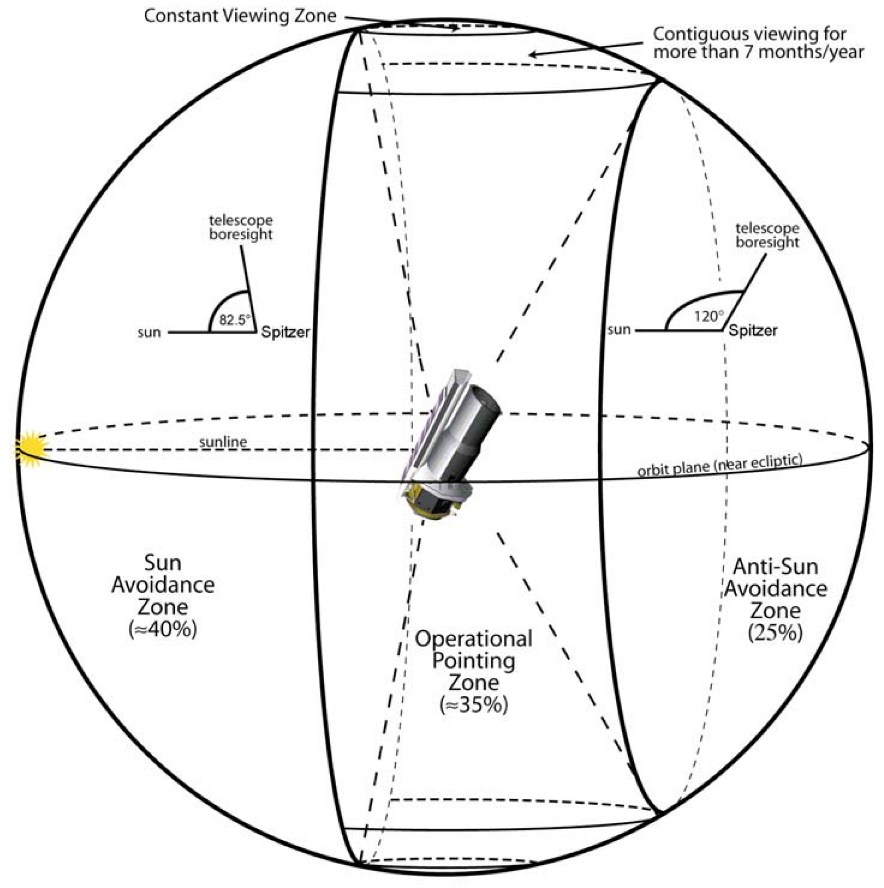
Figure 3: Depiction of the region into which Spitzer can point (Fig. from SOM, p. 26).

The permissible range of spacecraft attitude is severely constrained: The requirement to shield the spacecraft from direct sunlight virtually forbids “roll” rotations around telescope boresight (the roll angle is fixed to its nominal value ). Furthermore, telescope pointing is restricted to solar elongations above $82.5\text{\,}\mathrm{\SIUnitSymbolDegree}$ in order to prevent sunlight from entering the telescope, and to solar elongations below $120\text{\,}\mathrm{\SIUnitSymbolDegree}$ in order to guarantee sufficient electric power output from the solar panels. Rotations about the axis pointing towards the Sun, however, are unconstrained, resulting in a viewing zone of annular shape, at solar elongations between 82.5 and $120\text{\,}\mathrm{\SIUnitSymbolDegree}$; see Fig. 3. This has a profound influence on observations of Solar System objects, which will be discussed in sect. 4.

Spitzer is on an Earth-trailing heliocentric orbit, drifting away from Earth at a rate of about . It is thus not only far away from the Earth atmosphere, but also from its thermal environment, which would otherwise substantially heat up the spacecraft and thus limit the cryogenic lifetime. Also, this orbit limits the projected size of the Earth and Moon avoidance zones for telescope observations.

2 Optical design

The telescope has an aperture of $0.85\text{\,}\mathrm{m}$ and a focal ratio of $f/12$ (at $5.5\text{\,}\mathrm{K}$; focal length $10.2\text{\,}\mathrm{m}$) and follows the Ritchey-Chrétien variant of the Cassegrain design. It is entirely made of beryllium, a light metal of low heat capacity at low temperatures. Imaging is diffraction limited at wavelengths above $5.5\text{\,}\mathrm{\SIUnitSymbolMicro m}$.

There are no moving parts on the spacecraft, with the exception of the camera shutter of IRAC (which is, however, not being planned to be used in flight) and a mirror inside MIPS. The absence of (movable) camera shutters hampers calibration measurements, in particular dark current measurements, which will be discussed in the appropriate instrument sections.

Only one science instrument is powered up at any time, in order to minimize cryogen consumption due to dissipation of electric power. Instrument change-over entails a substantial amount of engineering and calibration activities. Instruments usually stay on for roughly one week, called an instrument campaign.

Spitzer has different mechanisms for changing and controlling telescope pointing which, in the absence of moving parts, is tantamount to spacecraft attitude. The accuracy of “blind” slews is $0.5\text{\,}\mathrm{\SIUnitSymbolArcsecond}$ ($1\sigma$), which is sufficient to acquire imaging targets but not always sufficient for spectroscopy. Relative pointing (for slews of up to $30\text{\,}\mathrm{\SIUnitSymbolArcminute}$) is more accurate. Pointing is stable to within $0.1\text{\,}\mathrm{\SIUnitSymbolArcsecond}$ ($1\sigma$) over $1000\text{\,}\mathrm{s}$. Spitzer is capable of linearly tracking moving targets of apparent velocities of up to $1\text{\,}\mathrm{\SIUnitSymbolArcsecond}\text{\,}{\mathrm{s}}^{-1}$, which is sufficient for all our programs.

3 Planning and proposing observations

The majority of Spitzer observing time is open to international observers in an open competition. General Observer (GO) proposals are invited by the Spitzer Science Center (SSC) on an annual basis in mid February, programs awarded observing time are scheduled within a 12-month period starting the following summer. Director’s Discretionary Time (DDT) is available for observations of unexpected phenomena of particularly high scientific merit which cannot be accommodated by GO programs. DDT can be applied for at any time on relatively short notice. Three out of our four Spitzer programs were GO programs, we were awarded DDT for one program.

All proposals must be submitted electronically to the SSC, along with a full specification of all proposed observations, using the SSC-supplied software SPOT (Spitzer Planning Observations Tool). SPOT can be used to determine times at which prospective targets are observable with Spitzer; Spitzer pointing is constrained in solar elongation (see sect. 1), neither may the telescope be pointed close to bright moving sources (planets, dwarf planets, the Moon, and the brightest asteroids) which may temporarily damage the detectors.

In SPOT, different types of constraints can be imposed on the relative or absolute timing of proposed observations, we will discuss some of these in sect. 4. Any timing constraint imposed must be given a scientific justification.

If an observing program is accepted, the parameters entered into SPOT are automatically transformed into commands uplinked to the spacecraft.

Due to Spitzer’s high sensitivity and accuracy, in the planning of observations effects must be considered which are unfamiliar from ground-based mid-infrared observations. For example, contamination due to faint background sources becomes a problem (see sect. 4), potentially leading to confusion noise. Furthermore, possible detector dysfunctionalities (e.g. due to cosmic ray hits or defective pixels) together with the non-interactive nature of Spitzer observations require imaging observations to be highly dithered, i.e. several consecutive observations of the target should be taken at small spatial offsets from one another. SPOT provides several instrument-specific templates for that. Dithering has the additional advantage of mitigating against any residual pixel-to-pixel variations in sensitivity not caught in the flat-fielding process.

4 Asteroid-specific aspects to observation planning

Parallax

Spitzer is not on a geocentric orbit, but trails behind the Earth on a heliocentric orbit at a steadily increasing geocentric distance. This causes a parallax between the Spitzer-centric and geocentric apparent positions of solar-system targets, particularly for near-Earth objects. Horizons, the JPL on-line ephemeris service (http://ssd.jpl.nasa.gov/?horizons), can be used to generate Spitzer-centered ephemerides of solar-system objects—the telescope code for Spitzer is $-79$.

Figure 4: Minimum solar phase angle, $\alpha_{\text{min}}$ for Spitzer observations of Solar System objects as a function of heliocentric distance, $r$ (see eqn. 1). Spitzer’s heliocentric distance $r_{\text{SST}}$ is assumed to equal .

Solar elongation constraints

As discussed in sect. 1, spacecraft design constrains telescope pointings to solar elongations between 82.5 and $120\text{\,}\mathrm{\SIUnitSymbolDegree}$. While for inertial targets this only constrains the time of their observability, for solar-system objects this prevents observations close to opposition (solar elongation of $180\text{\,}\mathrm{\SIUnitSymbolDegree}$), where it would be preferable to observe them. Not only do solar-system objects generally reach their peak brightness at opposition, but they are also best observable from ground during that time. The impossibility of close-to-opposition Spitzer observations thus hampers simultaneous ground-based support observations with, e.g., optical telescopes, which would have been advantageous for some of our programs. Most importantly, however, the solar elongation constraint provides a lower limit on the solar phase angle, $\alpha$, at which objects are observable—minimum phase angles occur at opposition. The importance of the phase angle for thermal modeling is discussed in sect. 5. The minimum solar phase angle $\alpha_{\text{min}}$ for Spitzer observations of solar-system objects is a function of their heliocentric distance $r$ and of Spitzer’s heliocentric distance $r_{\text{SST}}$:

$$\alpha_{\text{min}}(r)=\arcsin{\frac{\sqrt{3}}{2}\frac{r_{\text{SST}}}{r}},$$ (1)

where it is assumed that the minimum phase angle occurs at an elongation of $120\text{\,}\mathrm{\SIUnitSymbolDegree}$ (true for $r>r_{\text{SST}}$). See Fig. 4 on p. 4 for a plot.

Instrument change-over

Only one Spitzer instrument is powered up at any time. Therefore, multi-wavelength observations using different instruments entail a time gap between observations of a few hours at least, which may result in an additional flux uncertainty due to lightcurve effects.

Background sources

With ground-based mid-infrared telescopes such as the IRTF (see chapter 4), only very bright targets can be observed, which are virtually guaranteed to be the only observable source inside the FOV. This is different with Spitzer. Its high sensitivity leads to several potential problems, which need to be mitigated against in both observation planning and data analysis:

• Very bright background sources inside (or close to) the FOV heavily saturate the detector and compromise observations due to, e.g., blooming. The timing of asteroid observations must therefore be constrained to times where no such bright background source is near-by. This time-consuming task can be accomplished by overlaying star charts with the asteroid path using SPOT (see, e.g., Fig. 5 on p. 5). The most useful star charts for this purpose are those derived from the IRAS survey at wavelengths of 12 and $25\text{\,}\mathrm{\SIUnitSymbolMicro m}$. Most IRAS sources would heavily saturate Spitzer cameras in deep integrations.

• For deep imaging observations, the brightness of (spatially resolved or unresolved) background sources may be comparable to that of the asteroid target, causing difficulties for reliable target flux extraction in their vicinity. Although this latter effect is mitigated by the apparent motion of asteroids, it severely compromised several of our asteroid observations. Note that deep imaging observations regularly consist of a time series of individual pointings, during which the asteroid moves. Data can be partially recovered by rejecting frames with close asteroid-star encounters.

Other reasons for imposing timing constraints on asteroid observations may be target brightness (particularly for near-Earth objects, where brightness is a strong function of time) or phased observations of the asteroid lightcurve.

5 Spitzer data reduction

The SSC discourages observers from performing calibration observations; instead, calibration observations are regularly performed by members of the instrument teams along with maintenance operations. All science data are partially reduced at the SSC. To this end, the SSC hosts instrument-specific sets of automated partial data reduction routines, referred to as the BCD pipelines, where BCD stands for Basic Calibrated Data. The BCD pipelines remove most known instrument artefacts from the data and also perform absolute flux calibration. While raw data are made available to the observer, most parts of the BCD pipelines and most required calibration files are not.

The remaining data reduction steps to be taken by the observer include removal of residual instrument artefacts, stacking and coadding appropriate data subsets, extraction of target fluxes, and correction of target fluxes for, e.g., the effect of filter breadth. See the appropriate subsections of sect. 2 and 3.

2 InfraRed Array Camera (IRAC)

IRAC (acronym for InfraRed Array Camera) is an imaging camera at the low-wavelength end of Spitzer’s spectral coverage: It consists of four detectors operating at central wavelengths around 3.6, 4.5, 5.8, and $8.0\text{\,}\mathrm{\SIUnitSymbolMicro m}$ (referred to as channels 1–4 in the following). Each detector has a square field-of-view (FOV) 256 pixels wide, corresponding to roughly $5.2\text{\,}\mathrm{\SIUnitSymbolArcminute}$ at a pixel scale around $1.2\text{\,}\mathrm{\SIUnitSymbolArcsecond}$.

At IRAC wavelengths, reflected sunlight and thermal emission contribute to the observable asteroid flux. At $3.6\text{\,}\mathrm{\SIUnitSymbolMicro m}$ (channel 1), thermal flux is generally negligible relative to reflected sunlight, the converse applies to channel 4 ($8.0\text{\,}\mathrm{\SIUnitSymbolMicro m}$). The IRAC wavelength range is at the Rayleigh-Jeans tail of the emission of stellar background sources, therefore their brightness relative to that of asteroids decreases with wavelength.

This section starts with a short overview of the instrument layout and its capabilities as used in our observing programs (sect. 1). Our asteroid observation strategies are described in sect. 2. In the following two sections, we describe the employed data reduction techniques: First the partial, automated IRAC BCD pipeline hosted by the Spitzer Science Center (sect. 3), then the data reduction techniques employed by us (sect. 4). Sect. 5 is devoted to tests of our data reduction pipeline.

More information on instrument layout and nominal data quality can be found in Fazio2004, Hora2004, and in the IRAC data handbook provided on-line (IRACdatahandbook) (we made use of version 3.0 from 20 Jan. 2006, http://ssc.spitzer.caltech.edu/irac/dh/).

1 Instrument layout

Table 1: IRAC filter wavelengths and spectral breadths. See eqn. 7 on p. 7 for a definition of the effective wavelength.

	Channel 1	Channel 2	Channel 3	Channel 4
Mnemonic wavelength ( µ m )	3.6	4.5	5.8	8.0
Effective wavelength ( µ m )	3.550	4.493	5.731	7.872
FWHM ( µ m )	0.74	1.02	1.41	2.88
Relative filter width	21%	23%	25%	36%

IRAC consists of four CCD detectors sharing a common electronic and cryogenic framework. Channels 1 and 2 are In:Sb detectors, channels 3 and 4 are Si:As detectors. Filter wavelengths and spectral breadths for all channels are summarized in table 1. The detectors are situated inside the Cryogenic Telescope Assembly (see Fig. 2 on p. 2) at a helium bath temperature of $1.4\text{\,}\mathrm{K}$. All instrument control units are in the Spacecraft Bus. Each detector is 256 x 256 pixels in size, with a projected pixel size around $1.2\text{\,}\mathrm{\SIUnitSymbolArcsecond}$ x $1.2\text{\,}\mathrm{\SIUnitSymbolArcsecond}$. Each field of view (FOV) is about $5.2\text{\,}\mathrm{\SIUnitSymbolArcminute}$ x $5.2\text{\,}\mathrm{\SIUnitSymbolArcminute}$ wide. Channels 1 and 3 share a common aperture and FOV using a dichroic beam-splitter, the same applies to channels 2 and 4. The edges of the two FOVs are separated by about $1.5\text{\,}\mathrm{\SIUnitSymbolArcminute}$, so there is no overlap on the sky (see Fig. 5).

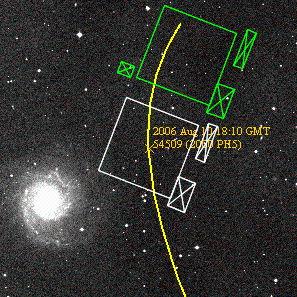
Figure 5: Projection of the two IRAC FOVs onto the sky: The FOV shared by channels 2 and 4 is depicted white, that of channels 1 and 3 is green. The crossed-out rectangles next to the FOVs represent the respective straylight-avoidance zones (see text). Depicted is a $$20\text{\,}\mathrm{\SIUnitSymbolArcminute}$\times$20\text{\,}\mathrm{\SIUnitSymbolArcminute}$$ patch of Digital Sky Survey (DSS) data centered at the position of (54509) YORP (then known under its provisional designation 2000 PH5) on 10 Aug 2006, 18:10 UT (yellow line and cross). The large spiral galaxy is Messier object 74 = NGC 628.

IRAC imaging is limited by diffraction with mean diffraction widths of $1.66\text{\,}\mathrm{\SIUnitSymbolArcsecond}$, $1.72\text{\,}\mathrm{\SIUnitSymbolArcsecond}$, $1.88\text{\,}\mathrm{\SIUnitSymbolArcsecond}$, and $1.98\text{\,}\mathrm{\SIUnitSymbolArcsecond}$ (FWHM) for channels 1–4, resp. With a pixel scale, the four IRAC point-spread functions are undersampled.

Table 2: IRAC point-source sensitivity ($1\sigma$ in units of µJy; see also eqn. 2 on p. 2) for one image frame of the stated integration time (frame time). The celestial background is assumed to be high, as is appropriate for most asteroid observations. Long exposures in channel 4 are background-limited; “$100\text{\,}\mathrm{s}$” frames in channel 4 are automatically converted into 2 frames of $50\text{\,}\mathrm{s}$ each.

Frame time (sec)	$3.6\text{\,}\mathrm{\SIUnitSymbolMicro m}$	$4.5\text{\,}\mathrm{\SIUnitSymbolMicro m}$	$5.8\text{\,}\mathrm{\SIUnitSymbolMicro m}$	$8.0\text{\,}\mathrm{\SIUnitSymbolMicro m}$
100	1.3	2.1	14	18
30	2.5	4.1	27	32
12	4.8	7.1	44	52
2	34	41	180	156

Table 3: Largest non-saturated point-source flux for the four IRAC channels and the stated frame times. Units in this table are m Jy, not µJy as in table 2! High celestial background is assumed.

Frame time (sec)	$3.6\text{\,}\mathrm{\SIUnitSymbolMicro m}$	$4.5\text{\,}\mathrm{\SIUnitSymbolMicro m}$	$5.8\text{\,}\mathrm{\SIUnitSymbolMicro m}$	$8.0\text{\,}\mathrm{\SIUnitSymbolMicro m}$
100	3.8	3.9	27	28
30	13	13	92	48
12	32	33	230	120
2	190	200	1400	740

In standard observing mode, there are four selectable options for the integration time per image frame (frame time) ranging from 2–$100\text{\,}\mathrm{s}$, see table 2 on p. 2 for the corresponding sensitivities and table 3 for the saturation limits. IRAC observations typically consist of a series of $n$ consecutive frames, which are later stacked; the total signal-to-noise ratio $S/N$ for a source with flux $f$ then equals

$$S/N(f)=\frac{f}{s}\sqrt{n}$$ (2)

where $s$ denotes the single-frame sensitivity $s$ as in table 2. For deep IRAC observations, the dominant source of uncertainty is celestial background radiation due to the emission and scattering of sunlight by zodiacal dust. The zodiacal dust is concentrated in the ecliptic plane, therefore IRAC’s sensitivity is a strong function of ecliptic latitude. We planned all observations assuming high background, as is appropriate for most Solar-System objects.

IRAC is continuously exposed to the sky; there is a shutter, which was used for laboratory measurements on ground, but it is not operated in flight in order to avoid any operational risk imposed by this moving part. Therefore, all four detectors take science quality data simultaneously. Even if only one channel is requested, the same field is observed in a second channel, while an adjacent (“serendipitous”) field is observed in the two remaining channels; for some purposes, we found it useful to obtain observations in one FOV by requesting observations of a suitably offset field with the other FOV (see sect. 2). Data from all four channels are processed through the BCD pipeline and made available to the observer.

IRAC is offset from the optical axis of the Spitzer focal plane (see Fig. 1 on p. 1) leading to optical distortion, i.e. the projected shape and size of pixels vary across the detector. The distortion has been modeled by the Spitzer Science Center to an accuracy of $0.1\text{\,}\mathrm{\SIUnitSymbolArcsecond}$ and must be corrected for in order to avoid significant photometric errors.

For all four IRAC channels, a certain amount of stray light is scattered onto the detectors. This is only critical if bright background sources are in certain “stray light avoidance zones” close to the FOV (see Fig. 5 on p. 5).

2 Observing strategy for asteroid photometry

IRAC observations have to be designed in a way quite different from ground-based mid-infrared observations:

• Observation design must be very robust because Spitzer executes all observations autonomously, without the possibility of real-time observer interaction. Also, the exact time at which observations are carried out is usually unknown at the planning stage—absolute timing constraints can be imposed by the observer but require a scientific justification. Once an observation is scheduled (roughly 2–5 weeks in advance), no more changes to the observation parameters can be made.

• Observations of faint targets are plagued by background sources of comparable brightness, the abundance of which grows rapidly with observation depth. While in the case of MIRSI, suitable targets are practically guaranteed to be the only observable source inside the FOV, IRAC observations must be designed in a way that mitigates against background contamination.

• There is also a non-negligible number of heavily saturating sources which, if inside the FOV, spoil the entire image frame and potentially subsequent image frames through latent effects. These must be prevented from entering the FOV.

IRAC observations are defined in the Spitzer Proposal Tool SPOT by specifying a target, the desired IRAC channels, the integration time per image frame, and the total number of image frames per channel to be taken. There are two options, which can be combined, for choosing the number of image frames: Dithering telescope boresight a user-defined number of times around the target location or identical in-place repeats. While dithering causes a small overhead for telescope slewing and settling, it enhances the accuracy and robustness of observations by mitigating against small-scale detector defects (e.g. permanently defective pixels or cosmic ray hits) and any residual pixel-to-pixel variations in sensitivity.

The timing of observations can be constrained by the observer in several ways, but it is stipulated in the Call for Proposals that they be minimized. Timing constraints require a compelling scientific justification, otherwise a lower priority will be assigned to the program by both the Time Allocation Committee and, if the program is accepted, in the scheduling queue.

Integration time

We determined the required total integration time from eqn. 2 on p. 2, depending on expected target flux and on our predefined goal for the total $S/N$ required to reach our scientific goals.

The expected flux of our asteroid targets at IRAC wavelengths depends on several, generally unknown, asteroid parameters such as diameter and apparent color temperature. This may induce a flux uncertainty of up to a factor of 10. The exact time of observations is not known at the planning stage, adding to the flux uncertainty.

For each target, we calculated upper and lower flux limits assuming appropriate end-members of the plausible range of physical properties and ephemerides. We requested conservatively deep integrations, such that we would barely reach our $S/N$-goal assuming the lower flux limit. We also checked against the appropriate IRAC saturation limits (see table 3 on p. 3).

Timing constraints

We generally had to prevent Spitzer from observing at undue times by imposing absolute timing constraints, i.e. by explicitly specifying times during which the observations should take place.

For all asteroid targets, we identified “avoidance times” during which the target path is close to bright known infrared sources, which would heavily saturate the detectors and potentially lead to temporary detector damage if they enter a FOV or a straylight avoidance zone. This was done by overlaying star charts resulting from the IRAS $12\text{\,}\mathrm{\SIUnitSymbolMicro m}$ survey with the projection of the IRAC FOVs and the Spitzer-centric asteroid path (note the parallax between Spitzer and Earth) throughout the times of Spitzer observability; see Fig. 6 for a typical example. To be sure, we considered every known IRAS source to be potentially damaging IRAC, due to its much higher sensitivity.

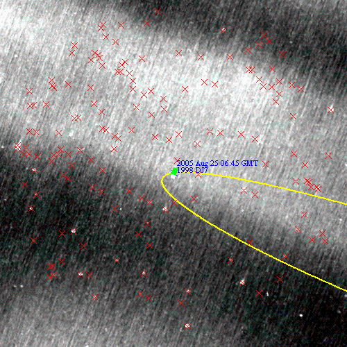
Figure 6: Star chart ($12.5\text{\,}\mathrm{\SIUnitSymbolDegree}$ $\times$ $12.5\text{\,}\mathrm{\SIUnitSymbolDegree}$) derived from the IRAS $12\text{\,}\mathrm{\SIUnitSymbolMicro m}$ survey, overlaid with the Spitzer-centric path of asteroid (33143) 1998 DJ7 (yellow line), known IRAS sources (red crosses) and the two IRAC FOVs (green and white as in Fig. 5 on p. 5, but note the size difference!).

Since heavy detector saturation may compromise subsequent observations through persistent latent images, we also kept the off-target FOV clear of IRAS sources.

Generally, this resulted in very mild timing constraints, typically barring a few hours per week, a notable exception being times during which the asteroid path intersects regions of high background source density, e.g. at low galactic latitudes.

For NEA targets, we additionally disabled observing at times when the target was too distant and thus too faint for successful observing.

Dithering

For most of our observations, telescope boresight is slightly altered between consecutive observations, such that the on-chip position of the target dithers around the FOV center. While this causes a slight overhead for telescope reorientation and settling, it helps mitigate against the effects of defective pixels or residual pixel-to-pixel variations in sensitivity.

SPOT provides several standard dither patterns. As recommended by the SSC, we generally chose mid-scale dither patterns, which keep our target on chip at all times. We generally chose the longest possible frame time ($100\text{\,}\mathrm{s}$) and the required number of dither positions to reach the total integration time previously determined (see sect. 2). We always used five or more dither positions, however, and therefore reduced the frame time for shallow observations.

For most deep IRAC observations, we employed a non-standard dither pattern in order to mitigate more efficiently against contamination from celestial background sources. For deep IRAC observations, practically no field in the sky is guaranteed to be clear of potentially interfering background sources, so it is impractical to avoid them by imposing timing constraints. Furthermore, unresolved faint background sources (or diffuse but structured emission, e.g. from zodiacal emission or galactic cirrus) decrease the accuracy at which photometry can be performed, leading to confusion noise which may limit the accuracy of deep IRAC observations.

This is mitigated against by the apparent movement of our targets: If the target moves by more than one PSF width between the first and last image in a series, then frames with background sources close to the asteroid path can be rejected (see sect. 4). Also, background structure is reduced by coadding image frames with different asteroid positions relative to the inertial background (see sect. 4).

To this end, we have designed deep asteroid observations in a highly redundant way, consisting of up to 144 on-target image frames per observation. In order to maximize the time baseline and thus the apparent asteroid motion between first and last frames, we have used a non-standard dither pattern. As opposed to the standard IRAC dither patterns, where the FOV shared by channels 2 and 4 is on target for the first half of the time, followed by the FOV of channels 1 and 3, we had the FOVs “take turns” on target up to ten times. This nearly doubled the temporal baseline at the expense of a small overhead for the additional telescope slews.

SPOT does not provide such dither patterns. We implemented them in an indirect way taking advantage of the IRAC peculiarity that even if only one channel is requested, all channels are exposed to the sky and read out, and all data are processed in the BCD pipeline. We requested a “moving cluster target” to be observed by channels 2 and 4, such that odd-number cluster positions are on target (not offset) and even-number cluster positions are offset by $402\text{\,}\mathrm{\SIUnitSymbolArcsecond}$ along the row axis in IRAC array coordinates, centering the 2nd FOV on target. Typically, a standard dither pattern is performed on each cluster position.

3 IRAC BCD pipeline

As for all Spitzer science data, IRAC data are partially reduced and calibrated at the SSC using an automated set of computer routines called the IRAC BCD pipeline (see sect. 5). It outputs one BCD file per pointing and detector, i.e. an image file in FITS format.

In this section, those aspects of the IRAC BCD pipeline which are relevant to our programs shall be sketched. The reference for most of the material presented here is the IRAC pipeline description document (IRACpipelinedescription).

Correction for dark current

An integration-time dependent dark-current estimate is subtracted from all images in the BCD pipeline. The detector dark-current levels for all possible integration times were determined on ground. In orbit, the absolute dark-current level cannot be measured since the shutter is not moved (see above). However, drifts in dark-current level are monitored based on sky dark frames, which are obtained from frequent, highly dithered observations of sky regions of very low emission (very low zodiacal background, only few bright sources such as stars).

First-frame effect

For an unknown reason, the dark-current level is a function of the time elapsed since the end of the previous detector readout, the so-called first-frame effect. This adds an unpredictable offset, chiefly to the first few frames in a series of observations. In order to mitigate against the first-frame effect, one or two redundant observing frames of short integration time are added by default at the beginning of each series of observations. The remaining background-level uncertainty is not corrected for in the BCD pipeline and must be considered in the data reduction, cf. sect. 4.

Flat-fielding

To correct for the pixel-to-pixel variation in sensitivity, IRAC science data are divided by a gain map over the FOV normalized to one, called a flat field. It is determined from frequent, highly dithered observations of predefined regions of high zodiacal emission (which is spatially relatively constant over the IRAC FOV; note again that IRAC’s shutter is not used in flight) and only small numbers of stars or galaxies. The images frames obtained are cleaned from localized sources and cosmic ray hits, then coadded and normalized to a median of one.

The flat-field frames thus obtained were seen to be constant within the observational uncertainty over the first two years of Spitzer operations.

Flux calibration

Flux calibration factors were determined from observations of a set of calibration stars before the beginning of normal science operations and are confirmed by regular reobservations (Reach2005). The absolute calibration accuracy is estimated to be within $3\text{\,}\%$, limited by the uncertainty in calibration star flux. The relative accuracy (temporal stability) of IRAC is $1.5\text{\,}\%$ (rms) over a year.

Calibration-star data-counts are obtained via synthetic aperture photometry using a particular set of aperture and sky-annulus radii (aperture radius: $10\text{\,}\text{pixels}$, annulus radii: 10 and $20\text{\,}\text{pixels}$); IRAC data should be reduced using the same parameters.

For the reduction of most deep observations these parameters are impractical. Smaller aperture and sky annulus radii can be used, but flux values thus obtained require a so-called aperture correction to be applied (see sect. 4).

The calibration procedure assumes targets to be point-like; this is a safe assumption for our asteroid targets, since their angular size is well below the IRAC diffraction widths.

IRAC is a broad-band photometer (see table 1 on p. 1). In order to convert the passband-integrated detector response into monochromatic flux values at the effective filter wavelengths, assumptions must be made on the target spectrum. BCD fluxes are corrected for a spectrum inversely proportional to wavelength. Different target spectra require color corrections to be made, which can be significant in the case of asteroids (see sect. 4).

Calibrated images are in units of flux per solid angle. Note that this is not equivalent to flux per pixel due to distortion (see above).

Pointing refinement

Spitzer’s nominal pointing accuracy is $0.5\text{\,}\mathrm{\SIUnitSymbolArcsecond}$, less than half the width of an IRAC pixel. The astrometric accuracy of taken image frames is further refined to an accuracy of $0.15\text{\,}\mathrm{\SIUnitSymbolArcsecond}$ by matching the positions of detected sources with star catalogs (usually the 2 Micron All Sky Survey, 2MASS), more than sufficient for our needs.

4 Data reduction steps taken by us

We start our data reduction efforts at the BCD stage. First, unusable or irrelevant (off-target) BCD frames are filtered out. This includes visual inspection of all image frames (see sect. 4).

Then, the remaining BCD files belonging to one observation are coadded to a mosaic image in the asteroid rest frame. This includes several image manipulation tasks in order to mitigate against celestial background structure and to remove further detector effects and transient artefacts such as cosmic ray hits. These are described in sections 4 and 4.

Asteroid fluxes are determined from the mosaic images. This includes several corrections for known detector or source properties (see sections 4 through 4).

All IRAC BCD files considered in this thesis were produced by the BCD pipeline version 14. For mosaicking, the software package MOPEX was used. MOPEX is provided by the SSC (http://ssc.spitzer.caltech.edu/postbcd/download-mopex.html; we used the version for Linux named 030106, released on 1 March 2006).

Filtering frames

Image frames that were irrelevant or unusable for our purposes were rejected from further analysis after visual inspection.

Due to IRAC’s design with two non-overlapping fields-of-view (see Fig. 5 on p. 5) constantly exposed to the sky, the fields-of-view “take turns” on the target in a user-defined way when observing a point source in all four channels. Therefore, half of the downloaded image frames are off target and irrelevant for our purposes. Those were deleted, which significantly saved on storage space—and on computer time during sub-sequent analyses.

Also, as introduced in sect. 3, each series of IRAC observations starts with one or two redundant integrations of reduced integration time in order to mitigate against the first-frame effect. Those images were deleted.

We visually inspected each remaining image frame before further analysis in order to reject unusable frames. Those include frames with very bright on-chip sources (or particularly bad cosmic ray hits) compromising the image quality throughout the detector through blooming effects. Also frames with detector artefacts, cosmic ray hits, or background sources within a few pixels from the target location were rejected. Generally, only parts of the data were affected due to dithering and the apparent movement of the asteroid target relative to the fixed star background.

Background matching

The first-frame effect (sect. 3) is a drift of the background levels in a series of observations, causing difficulties for outlier rejection during mosaicking (cf. sect. 4). First frames in a series are most affected.

Although the first frame is always rejected (see above), it is nevertheless required to match the background levels of image frames to be mosaicked. This is accomplished using the program overlap.pl, which is part of the MOPEX package. It determines an offset value to each input image such that the pixel-by-pixel difference between overlapping areas of pairs of input images is minimized.

In a first step, the program reprojects and interpolates the BCDs onto a common rectangular grid. In a second step, bright sources above a user-specified detection threshold, particularly cosmic ray hits, which would bias the overlap correction, are masked and excluded from further processing. Then the additive overlap corrections are calculated and the corrected images are saved.

The detection threshold for bright object masking must be adjusted on a case-by-case basis, after evaluation of the mosaicking process.

Mosaicking and outlier rejection

Generally, IRAC observations are not performed as a single frame of the required integration time, but rather as a set of at least 5 correspondingly shorter integrations (our deepest IRAC observation consists of 144 individual BCD frames). Usually, telescope boresight of the individual observations is slightly altered between consecutive observations, such that the on-chip position of the target dithers around the FOV center (see sect. 2). Deriving target fluxes thus requires combining these exposures into a single high signal-to-noise image, referred to as mosaic.

Mosaicking is the most time-consuming part of IRAC data reduction, both in terms of computer time and number of iterations generally required to achieve a satisfactory result. We use the program mosaic.pl, part of the software package MOPEX, for this task. Mosaicking is done in three consecutive steps:

Reprojection

Image data are reprojected and interpolated onto a common rectangular grid with a pixel scale of $1.20\text{\,}\mathrm{\SIUnitSymbolArcsecond}$. In particular, the effects of optical distortion are taken into account.

The asteroid rest frame is used as reference frame, i.e.  the asteroid position is constant on all reprojected images while the positions of inertial background sources vary. In some of our observations, background star trails are longer than $10\text{\,}\mathrm{\SIUnitSymbolArcsecond}$.

Outlier rejection

Outlier pixels containing anomalously high or low signal are detected and rejected. These may be due to cosmic ray hits or detector artefacts, which may be permanently bad pixels or in response to a previous over-exposure, e.g. due to a cosmic ray hit (see IRACdatahandbook). Also non-co-moving sources are partially rejected.

Outlier detection is based on pixel-wise image-to-image comparison. MOPEX provides three complementary algorithms for that; careful parameter tuning on a case-by-case basis is required in order to reliably reject outliers while keeping legitimate sources. It is crucial to inspect the maps of rejected pixels and to visually compare them with the input images in order to gage the quality of outlier rejection—the Airy rings around targets, in particular, are in danger of being erroneously rejected. Several reiterations may be required. If background matching was not well performed (see sect. 4), large parts of one input image may be flagged as outliers, requiring a reiteration of that step, too.

Coaddition

A mosaic is generated by pixel-wise averaging those parts of the input images flagged as good. Also a coverage map is generated, indicating the number of good input image pixels used for each output pixel. Coverage maps are particularly useful for gaging the quality of mosaics.

Automated source extraction and photometry using MOPEX

MOPEX contains a program to automatically determine the position and absolutely calibrated brightness of point sources called APEX. APEX fits segments of mosaic images with the point-spread function, which is constant over time to a high accuracy. If a satisfactory fit is reached, APEX assumes a detection and determines the source flux by scaling the point-spread function and (if requested by the user) fitting the background.

Using APEX for flux determination is not generally recommended by the SSC (since flux calibration is performed using synthetic aperture photometry), but considered preferable inside fields containing many point sources: In the case of two or more sources whose point-spread functions overlap significantly, synthetic aperture is futile, whereas point-spread-function fitting still has a certain chance of success.

While we could determine flux values of calibration standard stars using APEX (c.f. sect. 5), we got no meaningful results in the case of asteroids with near-by stellar sources. We reckon the reason for this is the movement of the asteroid targets relative to the inertial background: While on mosaic images the point-spread function is probably a good match to the image of the asteroid itself, the trails of background stars are only poorly matched.

Synthetic aperture photometry

Instead, we extracted asteroid flux densities from mosaicked images using the synthetic aperture photometry routines used for the analysis of IRTF data (see sect. 1; the software has been developed by M. Delbo2004). We generally used different combinations of aperture and sky annulus radii for which aperture correction factors were available (see sect. 4). Structure in the celestial background (e.g. background stars) often necessitated using small radii for both aperture and sky annulus. This effect is more severe in the short-wavelength channels 1 and 2 (the relative brightness of asteroids is larger in channels 3 and 4).

Before extracting fluxes, we converted the units of mosaic images from M Jy/ sr  into µJy/pixel, such that the photometry output is in units of µJy.

Aperture correction

Let $f_{i,j,k}$ denote the flux contained in an aperture of radius $i$ minus the sky background content estimated from the flux inside an annulus of inner radius $j$ and outer radius $k$ (all radii in pixels). In general, $f_{i,j,k}$ is a function of $i$, $j$, and $k$: Varying $i$ changes the percentage of the point-spread function (PSF) energy content contained in the aperture, small values for $j$ and $k$ imply that parts of the source flux are inside the sky annulus, leading to sky-background overestimation and hence flux underestimation.

By virtue of the IRAC flux calibration scheme (see sect. 3), $f_{10,10,20}$ is generally the best available approximation to the “true” flux $f_{\text{true}}$. Structure in the celestial background, however, often renders it impractical to use such large radii (see above). Fortunately, due to the high temporal stability of the IRAC PSFs, the ratio $f_{10,10,20}/f_{i,j,k}$ is very stable, such that smaller radii can safely be used if the resulting flux is later multiplied by the appropriate aperture correction factor $AC_{i,j,k}$:

$$f_{10,10,20}\sim AC_{i,j,k}f_{i,j,k}.$$ (3)

Table 4: Aperture correction factors $AC_{i,j,k}$ for the four IRAC channels and different aperture and sky annulus radii $i$, $j$, and $k$ (in mosaic pixels, $1.20\text{\,}\mathrm{\SIUnitSymbolArcsecond}$ each), see eqn. 3. The values in this table are assumed to be accurate to roughly one percent and differ slightly (but significantly) from those given in the IRAC data handbook (p. 53) due to the different pixel sizes used (see sect. 5).

Aperture	Sky annulus	Channel 1	Channel 2	Channel 3	Channel 4
2	2–6	1.253	1.278	1.414	1.615
2	10–20	1.236	1.259	1.393	1.582
3	3–6	1.128	1.133	1.154	1.255
3	10–20	1.110	1.114	1.131	1.235
5	5–10	1.057	1.067	1.065	1.081
5	10–20	1.043	1.049	1.050	1.060
10	10–20	1.000	1.000	1.000	1.000

Aperture correction factors are obviously dependent on the pixel scale. Those quoted in the IRAC datahandbook (p. 53) are for a pixel scale around $1.22\text{\,}\mathrm{\SIUnitSymbolArcsecond}$ and therefore not directly applicable to us, since we use a mosaic pixel scale of $1.20\text{\,}\mathrm{\SIUnitSymbolArcsecond}$. We have therefore determined aperture correction factors to be used with our mosaic pixel scale of $1.20\text{\,}\mathrm{\SIUnitSymbolArcsecond}$ from observations of the bright star HD 165459, which is also used as an IRAC photometric calibration standard (see also sect. 5). See table 4 for our results, which we estimate to be accurate to roughly one percent, limited by the statistical uncertainty of the star flux determinations.

Note that this procedure can only be used in the case of a high temporal PSF stability—it cannot be used for, e.g., mid-infrared asteroid imaging using the IRTF (where the PSF depends on variable parameters such as seeing or telescope focus).

Color correction

IRAC is a broad-band photometer. Derivation of monochromatic flux values from the detector output therefore requires assumptions on the target spectrum to be made and an appropriate choice of the effective filter wavelength $\lambda_{0}$. Flux values obtained so far are correct for a nominal source spectrum $f_{nom}(\lambda)\propto\lambda^{-1}$ (with wavelength $\lambda$) (see sect. 3). For other target spectra, this causes a systematic multiplicative offset, requiring a color correction to be made. Color correction factors for several target spectra are tabulated in the IRAC data handbook, p. 48 (IRACdatahandbook), but none of them is directly applicable to our asteroid targets.

When observing a source with flux distribution $f(\lambda)$, the detector response per integration time, $R$, equals

$$R=f\left(\lambda_{0}\right)\int\frac{f\left(\lambda\right)}{f\left(\lambda_{0}\right)}\frac{R\left(\lambda\right)}{hc/\lambda}\text{d}\lambda$$ (4)

with the spectral detector response $R(\lambda)$ in units of electrons per photon (hence the division by the photon energy $hc/\lambda$; all integrals in this section run from 0 to $\infty$). The detector response to a target with spectrum $f_{tar}(\lambda)$, $R_{tar}$, and that to a calibration star with spectrum $f_{cal}(\lambda)$, $R_{cal}$, are then related to the monochromatic flux densities at the wavelength $\lambda_{0}$:

$$f_{tar}(\lambda_{0}) =f_{cal}(\lambda_{0})\frac{R_{tar}}{R_{cal}}\times K$$ (5a)

$$K =\frac{f_{tar}(\lambda_{0})}{f_{cal}(\lambda_{0})}\frac{\int f_{cal}(\lambda)R(\lambda)/(hc/\lambda)\text{d}\lambda}{\int f_{tar}(\lambda)R(\lambda)/(hc/\lambda)\text{d}\lambda}$$ (5b)

with the color-correction factor $K$ taking account of the differences in spectral shape through the detector passband. Note in particular that $K$ is invariant under rescaling of both $f_{tar}$ and $f_{nom}$.

The IRAC BCD flux calibration includes a color correction assuming a nominal source spectrum $f_{nom}(\lambda)\propto\lambda^{-1}$. This requires a second color correction to be made:

$$f_{tar}(\lambda_{0}) =\frac{f_{nom}(\lambda_{0})}{K}$$ (6a)

$$K =\frac{f_{nom}(\lambda_{0})}{f_{tar}(\lambda_{0})}\frac{\int f_{tar}(\lambda)R(\lambda)/(hc/\lambda)\text{d}\lambda}{\int f_{nom}(\lambda)R(\lambda)/(hc/\lambda)\text{d}\lambda}.$$ (6b)

Table 5: IRAC color-correction factors for NEATM asteroid spectra for several heliocentric distances $r$ (in AU), solar phase angles $\alpha$ (in degrees), model parameters $\eta$, and geometric albedos $p_{\text{V}}{}$ (the slope parameter $G$ is assumed to equal 0.15). The last column refers to the section in which the thus calculated color-correction factors are required.

$r$	$\alpha$	$\eta$	$p_{\text{V}}{}$	Channel 1	Ch. 2	Ch. 3	Ch. 4
1.00	60.0	2.0	0.2	1.138	1.070	1.033	1.003	Sect. 4
1.27	52.33	2.48	0.35	1.236	1.129	1.070	1.034	Sect. LABEL:sect:ML

We have developed a computer routine which calculates color correction factors for all IRAC channels and several model spectra, including NEATM asteroid spectra with variable model parameters. It makes use of the measured spectral response curves of each IRAC detector tabulated on-line by the SSC (http://ssc.spitzer.caltech.edu/irac/spectral_response.html). We have verified that our software reproduces all color correction factors quoted in the IRAC handbook (p. 48) to within one percent. See table 5 for IRAC color correction factors for NEATM spectra with several model parameters.

The values of $\lambda_{0}$ used in the IRAC BCD pipeline were chosen in a way that minimizes the dependence of color-correction factors on the spectral slope. They are defined the following way:

$$\lambda_{0}=\frac{\int R(\lambda)\text{d}\lambda}{\int R(\lambda)/\lambda\text{d}\lambda}.$$ (7)

Evaluation of this integral for the four tabulated IRAC passbands yields effective wavelengths of 3.550, 4.493, 5.731, and $7.872\text{\,}\mathrm{\SIUnitSymbolMicro m}$ (see table 1 on p. 1).

Estimation of flux uncertainty

We estimated the statistical flux uncertainty in two mutually independent ways, which we added in quadrature:

• The standard statistical flux uncertainty derived from the scatter in the background flux level

• The scatter in the aperture-corrected fluxes derived using different possible radii for the synthetic aperture and the sky annulus (see sect. 4). This scatter is estimated to be a measure of the PSF deviation from its nominal form due to background structure or noise.

The accuracy of observations in channels 1–3 was generally limited by statistical uncertainty, while our highest signal-to-noise channel-4 observations were occasionally limited by the $3\text{\,}\%$ (Reach2005) calibration uncertainty.

On the basis of our data reduction pipeline validation experiments described in sect. 5 we estimate that our data reduction pipeline does not introduce major systematic uncertainties. We therefore neglect any systematic uncertainties resulting from, e.g., aperture correction (sect. 4) or color correction (sect. 4).

5 Validation of our data reduction pipeline

Table 6: Fluxes of the photometric calibration standard star HD 165459 from IRAC observations on 13 February 2006 (upper row) and expected values (lower row, quoted from Reach2005, Table 6). Values in the upper row are not color-corrected to enable comparison with the Reach2005 values. Uncertainties in the first row are statistical (from the synthetic aperture procedure), those in the second row are systematic (uncertainties in stellar flux modeling).

	Channel 1	Channel 2	Channel 3	Channel 4
	( m Jy)	( m Jy)	( m Jy)	( m Jy)
Determined	$643.9\pm 4.1$	$410.2\pm 7.3$	$264.3\pm 8.2$	$147.0\pm 2.6$
Expected	$647\pm 17$	$421\pm 11$	$268.7\pm 7.1$	$148.1\pm 3.9$

Check against a calibration star

We have validated our data reduction pipeline by determining flux values which were known a priori: The brightness of a star used in the photometric calibration of IRAC. A list of such stars and their fluxes at IRAC wavelengths has been published by Reach2005. We have searched the database of publicly available Spitzer data and retrieved IRAC observations of the calibration standard star HD 165459 taken on 13 Feb 2006; the on-target integration time per FOV was 5 dither positions times $2\text{\,}\mathrm{s}$. These observations were performed as part of a regular IRAC calibration program; the downloaded data were processed through the standard IRAC BCD pipeline.

We have determined flux values for the four IRAC channels using the method described in this section without color correction. As can be seen in table 6, fluxes agree with those given by Reach2005 within the error bars.

Check pixel-scale effects

We use a mosaic pixel scale of $1.20\text{\,}\mathrm{\SIUnitSymbolArcsecond}$, while a pixel scale of $\sim 1.22$ ″ is used for IRAC calibration. Note that the photometric calibration is tied to synthetic aperture photometry with an aperture of 10 pixels, so the pixel scale would be expected to matter.

In order to verify that this does not introduce an appreciable calibration uncertainty, we have mosaicked the above-mentioned HD 165459 data twice, using pixel scales of 1.20 and $1.22\text{\,}\mathrm{\SIUnitSymbolArcsecond}$, respectively. Fluxes resulting from synthetic aperture photometry (with “default” radii of 10, 10, and 20 pixels) agree to within a few permille.

We have also determined aperture correction factors on the $1.22\text{\,}\mathrm{\SIUnitSymbolArcsecond}$ pixel scale mosaics using the method described in sect. 4. As expected, the thus determined aperture correction factors differ significantly from those quoted in table 4 on p. 4, but match those tabulated in the IRAC datahandbook, p. 53, to within $1\text{\,}\%$.

3 InfraRed Spectrograph (IRS)

The InfraRed Spectrograph (IRS; see IRS) covers the mid-wavelength range of Spitzer’s spectral coverage with spectroscopic capabilities over the wavelength range from 5.3 to $38\text{\,}\mathrm{\SIUnitSymbolMicro m}$ at two different spectral resolutions (referred to as low and high resolution in the following); and additional small-FOV imaging capabilities (peak-up imaging, PUI) at central wavelengths around 16 and $22\text{\,}\mathrm{\SIUnitSymbolMicro m}$. At IRS wavelengths, asteroid flux is practically purely thermal.

After a short overview of the instrument over-all layout and its capabilities as used in our programs (sect. 1), we detail our observing strategies and data reduction techniques in section 2 and 3 for peak-up imaging and low-resolution spectroscopy, respectively. The high-resolution spectroscopy mode is not used in our programs and is generally disregarded in the following.

More information on the instrument can be found in IRS, the SOM, and in the IRS data handbook provided on-line (IRSdatahandbook) (we made use of version 2.0 from 1 Apr. 2006, http://ssc.spitzer.caltech.edu/irs/dh/). A technical reference for the IRS BCD pipeline (see sect. 5) is the IRS pipeline description (IRSpipelinedescription).

1 Instrument layout

Similar to IRAC, IRS is composed of four detectors, located in the Cryogenic Telescope Assembly at a helium bath temperature of $1.4\text{\,}\mathrm{K}$, and a set of control units located in the Spacecraft Bus at a higher temperature (see Fig. 2 on p. 2). The four blocked-impurity-band detectors have $128\times 128$ pixels each, two detectors cover the IRS wavelength range at low spectral resolution ($\lambda/\Delta\lambda$ between 64 and 128) and two at high resolution around 600. The two short-wavelength detectors are Si:As arrays and referred to as Short-Low (SL) and Short-High (SH) for low and high spectral resolution, respectively. Analogously, the long-wavelength detectors, Si:Sb arrays, are referred to as Long-Low (LL) and Long-High (LH). The low-resolution modules use single diffraction gratings, the high-resolution modules employ a cross-dispersed echelle layout. Light from the two imaging apertures is projected onto two designated fields on the SL chip, with an effective FOV of $$54\text{\,}\mathrm{\SIUnitSymbolArcsecond}$\times$81\text{\,}\mathrm{\SIUnitSymbolArcsecond}$$ each at a pixel scale around $1.8\text{\,}\mathrm{\SIUnitSymbolArcsecond}$ ($30\times 45$ pixels). The focal plane apertures of the IRS modules have no overlap on the sky; bringing a target from one aperture to another requires slewing the spacecraft since IRS does not have any moving parts.

The spectroscopy modules employ narrow slit designs, where the slit width equals the point-spread function (PSF) width at the largest wavelength—due to diffraction-limited imaging the PSF width increases with wavelength. The projected slit widths are $3.6\text{\,}\mathrm{\SIUnitSymbolArcsecond}$ (SL), $4.7\text{\,}\mathrm{\SIUnitSymbolArcsecond}$ (SH), $10.5\text{\,}\mathrm{\SIUnitSymbolArcsecond}$ (LL), and $11.1\text{\,}\mathrm{\SIUnitSymbolArcsecond}$ (LH).

Ground-based tests showed the photometric response of the detectors to be temporally stable within $1\text{\,}\%$. The absolute photometric accuracy of spectroscopic observations is typically limited by spill-over losses due to source mis-centering, which are reduced by a procedure called peak up (see below).

For science observations, the IRS detectors use a read-out system named “sample-up-the-ramp” whereby each pixel is read out non-destructively a number of times at the beginning of each measurement, and an equal number of times at the end of each measurement before the detector is reset. This reduces read-out noise and helps mitigate cosmic ray hits. It also enables meaningful data to be extracted from moderately saturated pixels, although at reduced signal-to-noise.

Peak up

The $1\sigma$ accuracy of blind Spitzer pointings is $0.5\text{\,}\mathrm{\SIUnitSymbolArcsecond}$ (see sect. 2 on p. 2), therefore significant parts of the PSF are at risk of being placed outside the slit, in particular for the narrow short-wavelength slits. Mis-centering of spectroscopy targets results in systematic underestimation of the absolute flux level and furthermore introduces a spurious spectral slope over the sub-module’s spectral range because the PSF broadens with wavelength, leading to larger losses.

IRS offers a mechanism, called peak up, to center spectroscopy targets in the slit more accurately, using more accurate small slews after refining spacecraft pointing on one of two dedicated imaging arrays called peak-up arrays. The latter are also used for photometric imaging in the PUI mode which is discussed in sect. 2. Peaking up also enables spectroscopy of targets with relatively large positional uncertainty, which would otherwise be impossible to acquire.

Peak up zeroes in on the brightest source within a $24\times 24$-pixel ($$43.2\text{\,}\mathrm{\SIUnitSymbolArcsecond}$\times$43.2\text{\,}\mathrm{\SIUnitSymbolArcsecond}$$) square centered at the nominal position of the peak-up target. The peak-up target can be the spectroscopy target itself or a near-by source whose position relative to the spectroscopy target is accurately known (see SOM, for details). The brightness of peak-up targets should be within 5– at $16\text{\,}\mathrm{\SIUnitSymbolMicro m}$ or 15– at $22\text{\,}\mathrm{\SIUnitSymbolMicro m}$, depending on the peak-up array selected.

2 Peak-Up Imaging (PUI)

Although originally designed for peak up only, the two peak-up FOVs can be used to provide science-quality photometry. Since Spitzer cycle II (summer 2005), Peak-Up Imaging (PUI) is an IRS operation mode fully supported by the Spitzer Science Center, which includes regular calibration observations and a dedicated BCD pipeline.

Light entering the two peak-up apertures is passed through suitable bandpass filters and then projected onto two designated parts of the SL detector, which are not used for spectroscopy. Both FOVs have a total size of $41\times 56$ pixels with significant vignetting at the boundaries; the un-vignetted part in either FOV is $30\times 45$ pixels corresponding to roughly $$54\text{\,}\mathrm{\SIUnitSymbolArcsecond}$\times$81\text{\,}\mathrm{\SIUnitSymbolArcsecond}$$ at a pixel scale around $1.8\text{\,}\mathrm{\SIUnitSymbolArcsecond}$. After a PUI observation, the entire SL chip is read out, providing low-resolution spectra in two orders and imaging in both peak-up fields. Only one of the four fields-of-view, however, is on a given point-source target, the others observe neighboring “serendipitous” fields.

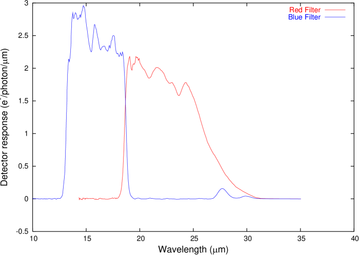
Figure 7: Detector response curves for the two IRS peak-up arrays. Depicted is the product of the total filter transmission and the spectral detector quantum efficiency, from the files linked at http://ssc.spitzer.caltech.edu/irs/spectral_response.html. Note the slight leak in the blue filter longward of $25\text{\,}\mathrm{\SIUnitSymbolMicro m}$.

See Fig. 7 for detector response curves for the two PU arrays. The effective wavelength of the “blue” filter is around $16\text{\,}\mathrm{\SIUnitSymbolMicro m}$, that of the “red” filter is about $22\text{\,}\mathrm{\SIUnitSymbolMicro m}$, the FWHM spectral breadth of either is some $30\text{\,}\%$.

Instrument performance

Table 7: PUI point-source sensitivity ($1\sigma$ in units of µJy; see also eqn. 2 on p. 2) for one image frame of the stated integration time (frame time). The celestial background is assumed to be high, as is appropriate for most asteroid observations.

Frame time (sec)	“Blue” filter ($16\text{\,}\mathrm{\SIUnitSymbolMicro m}$)	“Red” filter ($22\text{\,}\mathrm{\SIUnitSymbolMicro m}$)
30	80	120
14	120	180
6	190	280

Table 8: Largest non-saturated point-source flux (in units of m Jy) for the two PUI filters and high celestial background. Units in this table are m Jy, not µJy as in table 7! Note that imaging of somewhat brighter sources is possible regardless of saturation, although at reduced signal-to-noise, due to the sample-up-the-ramp read-out mode (see sect. 1).

Frame time (sec)	“Blue” filter ($16\text{\,}\mathrm{\SIUnitSymbolMicro m}$)	“Red” filter ($22\text{\,}\mathrm{\SIUnitSymbolMicro m}$)
30	35	80
14	80	190
6	180	410

Three values for the frame time, i.e. the integration time per frame, are selectable: 6, 14, and $30\text{\,}\mathrm{s}$. See table 7 for the corresponding point-source sensitivities and table 8 for the saturation limits. As in the case of IRAC (see sect. 2), longer integrations can be achieved by repeating frames in-place or by dithering; this will be discussed in sect. 2. For deep PUI observations, the dominant source of uncertainty is celestial background radiation due to the thermal emission of zodiacal dust which is concentrated in the ecliptic plane. Most of our asteroid observations took place at low ecliptic latitudes, hence we assumed the most conservative sensitivity values (“high” background) for planning of observations. In the IRS datahandbook (IRSdatahandbook, p. 50), systematic uncertainties in the PUI flux calibration are advertised to be within $6\text{\,}\%$ (see also sect. 2).

Similar to IRAC, PUI imaging suffers from a slight amount of optical distortion due to the instrument’s offset from the telescope optical axis. While less severe than in the case of IRAC (see sect. 1) due to the smaller field-of-view, distortion must be accounted for in the data reduction to avoid significant photometric errors.

Asteroid observation strategies

The design of our PUI observations was similar to that of our IRAC observations (see sect. 2)—note that all our PUI targets were also observed with IRAC.

Required integration times were estimated on the basis of the sensitivities given in table 7 and lower limits on expected target flux (see also sect. 2); a typical flux uncertainty at PUI wavelengths is a factor 3. Identical timing constraints were imposed on IRAC and PUI observations of the respective asteroid targets, thus preventing bright IRAS sources from temporarily damaging the detector through latent effects (see sect. 2). We typically dithered (see sect. 2) around the nominal target positions (4 or more dither positions) to mitigate cosmic ray hits and defective pixels; note that due to the limited FOV size, PUI dithering distances are much smaller than for IRAC.

BCD pipeline

As for all Spitzer science data, PUI data are partially reduced and calibrated at the Spitzer Science Center (SSC) using an automated set of computer routines called the PUI BCD pipeline (see sect. 5). The PUI BCD pipeline is mutatis mutandis nearly identical to the IRAC BCD pipeline (see sect. 3), we here sketch the former, focusing on differences among the two. One BCD file per filter and pointing is produced, i.e. a FITS file with most known instrument artefacts removed and in physical flux units ( M Jy/ sr ). Each BCD file is associated with several ancillary files including maps of estimated flux uncertainty and masks where potentially unreliable pixels are flagged (e.g. suspected cosmic ray hits, vignetted pixels, and permanently damaged pixels); those ancillary files are useful for further data reduction. Technical references for the PUI BCD pipeline are the IRS pipeline description (IRSpipelinedescription) and the IRS datahandbook (IRSdatahandbook).

Corrections for dark current are determined as in the case of IRAC (see sect. 3), but no time-dependent drift has been found, i.e. there is no first-frame effect (see sect. 3). PUI data are flat-fielded similar to IRAC data (see sect. 3) and flux calibrated against a set of stellar calibrators (see sect. 3 and SOM, p. 178; flux calibration will be further discussed in sect. 2). As in the case of IRAC, PUI data are flux calibrated assuming a target spectrum inversely proportional to wavelength, necessitating color corrections to be made (see sect. 2). Pointing refinement, as is done for IRAC data (see sect. 3), is not performed on PUI data; it would not be feasible in general due to the low density of bright stars at PUI wavelengths.

All IRS detectors including the SL chip used for PUI are subject to the damaging effects of solar flares, resulting in an increasing number of permanently or temporarily defective pixels. As a part of calibration activities, the SSC monitors the pixel responsivity and flags permanently damaged pixels as “dead” in the BCD pipeline. Some pixels, called “rogue pixels,” are overly responsive at times, but operate normally most of the time. The SSC issues regularly updated lists of rogue pixels, but rogue pixels are not flagged in BCD files.

Data-reduction steps taken by us

Reduction of PUI data is largely analogous to IRAC data reduction (see sect. 4). The most significant differences are the following:

Visual inspection

While all PUI data frames were visually inspected, no unusable PUI frames were found. This is due to the much lower density of bright stars at PUI wavelengths relative to IRAC wavelengths, but also due to the sample-up-the-ramp read-out mode (see sect. 1) mitigating the effects of cosmic-ray hits. Rogue pixels (see sect. 2), however, are clearly recognizable as such in visual inspection. It turned out to be easier to manually add them to the bad-pixel map provided by the BCD pipeline than to tweak the mosaic routines (see below) to reliably recognize rogue pixels without falsely flagging good pixels. To lighten this task, an IDL routine was developed which flags a rogue pixel for all BCDs belonging to a series of consecutive observations.

Background matching

Since no first-frame effect is present, background matching (see sect. 4) is not needed.

Mosaicking

A mosaic pixel scale of $1.8\text{\,}\mathrm{\SIUnitSymbolArcsecond}$ is used. Generally, no cosmic-ray hits or background sources are present in BCD images. Rogue pixels were rejected manually (see above). It is important to have mosaic.pl disregard pixels in the vignetted region close to the FOV boundary, where no reliable flat fielding is possible. They are flagged as vignetted in the BCD-provided bad-pixel map but not rejected by default.

Flux extraction, aperture correction, color correction

The PUI flux calibration is based on synthetic aperture photometry using a sky annulus with inner and outer radii of 8 and 14 pixels, respectively, and aperture radii of 3 (blue) and 4 (red) pixels (IRSdatahandbook). These aperture radii are small compared to the FWHM width of the PSF, which is around 2 (blue) and 2.5 (red) pixels, hence fluxes are aperture corrected by default. We generally used larger aperture radii and the quoted sky annulus radii; see table 9 for aperture correction factors. See table 10 for color-correction factors which were determined like their IRAC counterparts (see table 5 on p. 5) but using the PUI detector response (see Fig. 7 on p. 7).

Table 9: Aperture correction factors $AC_{i,j,k}$ (see eqn. 3 on p. 3) for the two PUI filters and different aperture radii (in mosaic pixels of $1.8\text{\,}\mathrm{\SIUnitSymbolArcsecond}$ each). Inner and outer sky annulus radii are 8 and 14 pixels, respectively. (from IRSdatahandbook, p. 50)

Aperture	Blue filter	Red filter
2	1.69	2.13
3	1.38	1.57
4	1.16	1.36
5	1.07	1.18
6	1.05	1.07
7	1.04	1.03
8	1.03	1.02
9	1.02	1.02
10	1.01	1.01
11	1.00	1.01
12	1.00	1.01

Table 10: IRS PUI color-correction factors for NEATM asteroid spectra for several heliocentric distances $r$ (in AU), solar phase angles $\alpha$ (in degrees), model parameters $\eta$, and geometric albedos $p_{\text{V}}{}$ (the slope parameter $G$ is assumed to equal 0.15). The last column refers to the section in which the thus calculated color-correction factors are required. The effective wavelengths were calculated from eqn. 7 on p. 7.

$r$	$\alpha$	$\eta$	$p_{\text{V}}{}$	Blue ($15.8\text{\,}\mathrm{\SIUnitSymbolMicro m}$)	Red ($22.3\text{\,}\mathrm{\SIUnitSymbolMicro m}$)
1.00	60.0	2.0	0.2	0.982	0.994	Sect. 4

Validation

We aimed at validating our PUI data reduction pipeline, like we have validated our IRAC pipeline (see sect. 5). However, as of April 2007, the Spitzer Science Center has not announced which flux standards were used for PUI flux calibration. Upon request, the Spitzer helpdesk informed us (private email communication from 24 Feb 2006) that the primary flux standard used for PUI calibration was the star HD 163466, with PUI fluxes of (blue) and (red) before color correction (similar to the IRAC calibration standard quoted in sect. 5).

PUI observations of that star were performed on 20 Apr, 26 Apr, and 26 May 2006 during regular IRS calibration observations, data are public. BCD files from these three observations were reduced by us using the data reduction pipeline described herein. The resulting flux values and their deviations from the nominal values are given in table 11.

Table 11: Determined fluxes of the star HD 163466, which was used for PUI flux calibration, from PUI observations on 20 Apr, 26 Apr, and 26 May 2006. Fluxes should be (Spitzer helpdesk, private email communication from 24 Feb 2006): (blue) and (red) before color correction.

Date	“blue” flux	off by	“red” flux	off by
	( m Jy)	(%)	( m Jy)	(%)
2006/04/20	$51.06\pm 0.30$	-5.9	$28.61\pm 0.16$	+4.3
2006/04/26	$50.98\pm 0.41$	-6.1	$28.86\pm 0.13$	+5.2
2006/05/26	$51.57\pm 0.47$	-5.0	$28.95\pm 0.17$	+5.5

We see significant deviations from the nominal values, roughly $-5.5\text{\,}\%$ in the blue filter and roughly $+5\text{\,}\%$ in the red filter. We have reported this discrepancy to the Spitzer helpdesk over summer and fall 2006. The helpdesk found no flaw in our data reduction pipeline but stated that our deviation in photometric zeropoints was well within the quoted uncertainty of . We feel, however, that our results reveal a rather serious calibration issue with the BCD pipeline 14, possibly related to the fact that flux calibration is tied to synthetic aperture photometry with very small radii, leading to relatively large uncertainties due to the needed aperture correction.

It should also be noted that in PUI observations of an exoplanet, repeated over a timespan of $6\text{\,}\mathrm{h}$, Deming2006 found a time dependent drift in PUI photometric gain, which cannot be explained to date.

Update: pipeline version 15

The validation attempt presented in this section is based on the IRS BCD pipeline version 14, issued in Jul 2006. The Spitzer Science Center has issued an updated IRS BCD pipeline, version 15, on 28 Feb 2007 “which results in changes in measured photometric values of $<$15\text{\,}\%$$.” All PUI data in the archive (including ours) have been reprocessed; however, at the time of writing, no updated pipeline documentation is available. We hope that this new pipeline version fixes the issues found herein and we will reprocess all our PUI data based on the reprocessed BCDs. All PUI fluxes quoted in this thesis are therefore preliminary—updated PUI fluxes based on the IRS BCD pipeline version 15 will be used for journal publication.

3 Low-resolution spectroscopy

Two modules (named SL and LL) provide low-resolution spectroscopy at a relative spectral resolution between 64 and 128 at wavelengths between 5.2 and $38.0\text{\,}\mathrm{\SIUnitSymbolMicro m}$. Each module has two sub-apertures in its slit, bringing source light in 1st and 2nd diffraction order of its diffraction grating onto the respective chip. The two diffraction orders do not overlap on the chip (this is prevented using suitable bandpass filters in the optical path) nor on the sky. The telescope must be slewed in order to bring an observational target from one sub-slit into another. In total, four telescope pointings are required to observe a spectrum over the full low-resolution wavelength range, one per sub-slit. The projected slit widths of the two modules match the FWHM PSF widths at the largest wavelengths (Spitzer imaging is diffraction limited, hence the PSF width grows with wavelength). Their length is much larger, such that one-dimensional spatial resolution is acquired along the slit in addition to the spectral dimension. There is some spectral overlap among spectrally adjacent IRS modules and spectral orders, allowing spectra to be cross-checked. See table 12 for an overview of slit dimensions and spectral ranges.

Table 12: IRS low-resolution modules: Overview of spectral coverage, detector pixel scale, and projected slit dimensions. Note the slight spectral overlap between the sub modules. PUI is performed on the SL detector.

	Wavelength range	Pixel scale	Slit width	Slit length
SL 2nd order	$5.2--8.7\text{\,}\mathrm{\SIUnitSymbolMicro m}$	$1.8\text{\,}\mathrm{\SIUnitSymbolArcsecond}$	$3.6\text{\,}\mathrm{\SIUnitSymbolArcsecond}$	$57\text{\,}\mathrm{\SIUnitSymbolArcsecond}$
SL 1st order	$7.4--14.5\text{\,}\mathrm{\SIUnitSymbolMicro m}$	$1.8\text{\,}\mathrm{\SIUnitSymbolArcsecond}$	$3.7\text{\,}\mathrm{\SIUnitSymbolArcsecond}$	$57\text{\,}\mathrm{\SIUnitSymbolArcsecond}$
LL 2nd order	$14.0--21.7\text{\,}\mathrm{\SIUnitSymbolMicro m}$	$5.1\text{\,}\mathrm{\SIUnitSymbolArcsecond}$	$10.5\text{\,}\mathrm{\SIUnitSymbolArcsecond}$	$168\text{\,}\mathrm{\SIUnitSymbolArcsecond}$
LL 1st order	$19.5--38.0\text{\,}\mathrm{\SIUnitSymbolMicro m}$	$5.1\text{\,}\mathrm{\SIUnitSymbolArcsecond}$	$10.7\text{\,}\mathrm{\SIUnitSymbolArcsecond}$	$168\text{\,}\mathrm{\SIUnitSymbolArcsecond}$

IRS spectroscopy observations are specified in SPOT. Adjustable parameters are:

• Peak-up method and parameters (see sect. 1)

• Sub-modules to be used; if more than one module is selected, observations are ordered by wavelength with short wavelengths first, i.e. SL2, SL1, LL2, LL1 if all four low-resolution modules are selected

• Integration time per frame and sub-module, where possible choices are 6, 14, 60, and $240\text{\,}\mathrm{s}$ for the SL modules; 6, 14, 30, and $120\text{\,}\mathrm{s}$ for the LL modules

• Number of frames (“cycles”) to be taken at each position to increase the total integration time

There are two different spectroscopy modes: staring and mapping. Staring mode is primarily designed for point sources after successful peak up; in each sub-module the source is first placed at $33\text{\,}\%$ of the slit length, then at $66\text{\,}\%$, at each position the specified number of frames is taken—the total integration time is thus twice the number of cycles times the frame time. The purpose of this “nodding” strategy is to enable correction for diffuse background emission. In mapping mode, the source is placed at a selectable number of offsets parallel and/or perpendicular to the slit direction, where the angular offset distances are adjustable. The mapping mode was designed for spectral maps of extended sources, but is also useful for spectroscopy of sources which cannot be peaked up on (see sect. LABEL:sect:Patroclus).

Instrument performance

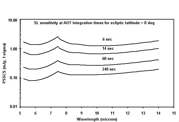
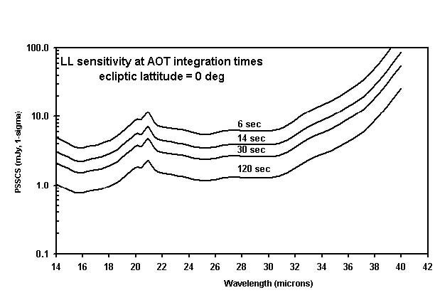
Figure 8: $1\sigma$ point-source sensitivity per frame for the SL (left) and LL (right) modules for the four possible frame times assuming low ecliptic latitude, i.e. high background due to zodiacal emission, as is appropriate for most asteroid observations. (Figs. from SOM, p. 160 and 161)

Table 13: Absolute photometric uncertainties due to spill-over losses for the SL and LL modules and the three selectable peak-up options. Note that the position uncertainty after a “low”-accuracy peak-up is actually worse than Spitzer’s nominal pointing accuracy; it should only be used on sources of poorly known position. (see SOM, p. 187)

	High	Moderate	Low
$1\sigma$ radial position uncertainty	$0.4\text{\,}\mathrm{\SIUnitSymbolArcsecond}$	$1.0\text{\,}\mathrm{\SIUnitSymbolArcsecond}$	$2.0\text{\,}\mathrm{\SIUnitSymbolArcsecond}$
Photometric uncertainty (SL)	$15--20\text{\,}\%$	$37--42\text{\,}\%$
Photometric uncertainty (LL)	$2--5\text{\,}\%$	$5--10\text{\,}\%$	$15--20\text{\,}\%$

See Fig. 8 for an overview of the sensitivities of the IRS low-resolution modules; the total signal-to-noise of an observation consisting of a series of $n$ frames is $\sqrt{n}\times f/s$ with flux $f$ and sensitivity $s$, provided other noise sources (e.g. shot noise) can be neglected. The maximum unsaturated flux is typically a few thousand times larger.

Laboratory tests on ground showed the temporal stability of the photometric response to an accurately centered source to be better than $1\text{\,}\%$; in flight, the photometric stability is limited by source mis-centering. The overall absolute photometric uncertainty of IRS is around $10\text{\,}\%$, dominated by uncertainty in stellar flux models (SOM, p. 210). See table 13 for an overview of photometric uncertainties due to spill-over losses.

Chapter 6 Results

This chapter contains results of thermal-infrared studies of 8 asteroids. Each of the eight sections is devoted to a self-contained study of an individual asteroid. Object-specific aspects of our results are discussed in the appropriate section, implications on asteroid science in general will be discussed in chapter LABEL:chapt:discussion.

The first five sections contain our main results: the thermal inertia, size, and albedo of 5 near-Earth asteroids (NEAs) with diameters spanning the range 0.1–$17\text{\,}\mathrm{km}$. These results are based on application of our thermophysical model (TPM; see chapter 3) to extensive sets of thermal-infrared data, most of which have been obtained using the IRTF (see chapter 4) or the Spitzer Space Telescope (see chapter 5). Section 1, in particular, contains a study of (433) Eros, which had been scrutinized using the NEAR-Shoemaker spacecraft. The primary aim of our Eros study is to validate the TPM for application to NEA data.

Sections LABEL:sect:Lutetia and LABEL:sect:ML contain studies of asteroid targets of future spacecraft encounters: (21) Lutetia, target of a flyby of the ESA spacecraft Rosetta in 2010, and (10302) 1989 ML, a nominal target of the planned ESA mission Don Quijote. Based on new thermal-infrared observations, these objects’ size and albedo have been determined, their surface mineralogy and thermal inertia have been constrained.

In section LABEL:sect:Patroclus, the first thermal-infrared observations of an eclipsing binary asteroid system, (617) Patroclus, are reported. These allowed us to determine the system’s thermal inertia in a fascinatingly direct way.

1 (433) Eros

In order to study the applicability of our thermophysical model (TPM) to NEAs, it was used to analyze published high-quality thermal-infrared data (HarrisDavies) of an extremely well studied object: (433) Eros, the NEA target of the rendezvous mission NEAR-Shoemaker.

We obtain a best-fit diameter of $17.8\text{\,}\mathrm{km}$, within of the NEAR-Shoemaker result of $16.9\text{\,}\mathrm{km}$ (Thomas2002). Depending on model assumptions, the best-fit thermal inertia is 100–$200\text{\,}\mathrm{J}\usk\power{\mathrm{s}}{-1/2}\power{\mathrm{K}}{-1}\power{\mathrm{m}}{-2}$, a very plausible value given the boulder-strewn yet regolith-dominated surface structure determined from spacecraft imaging, and furthermore in excellent agreement with previous estimates.

We conclude that the TPM is well suited to be applied to NEA data.

1 Introduction

Eros is a well studied object. E.g., the NEAR Shoemaker spacecraft scrutinized it for over one year while in orbit around Eros (see Veverka2000, and references therein). Thomas2002 report a regolith-dominated surface with a moderate amount of craters and boulders, and a volume of $2535\text{\,}{\mathrm{km}}^{3}$, corresponding to an effective diameter of $16.9\text{\,}\mathrm{km}$ (see eqn. 1 on p. 1). Eros’ disk-integrated albedo is $p_{\text{V}}{}=0.29\pm 0.02$ (at $\lambda=$550\text{\,}\mathrm{nm}$$) and $A=0.12\pm 0.02$ (Domingue2002). The exact spin state was determined by Thomas2002 along with an accurate model of its shape; the latter is available in a computer-readable format on-line at the Planetary Data System (http://pdssbn.astro.umd.edu/volume/nieros_4001/data/).

Eros’ thermal inertia has not been directly determined from spacecraft measurements. However, Eros was observed extensively during an exceptionally favorable close approach in 1974/75 enabling thermal studies of unprecedented detail (Morrison1976; LebofskyRieke1979). Although Eros’ shape had not been known in detail at that time, the authors could make use of detailed optical lightcurves available to them. Correcting the thermal lightcurve to the optical lightcurve (and allowing for a relative phase shift), Morrison1976 obtained an upper limit on thermal inertia around $100\text{\,}\mathrm{J}\usk\power{\mathrm{s}}{-1/2}\power{\mathrm{K}}{-1}\power{\mathrm{m}}{-2}$. LebofskyRieke1979, on the other hand, fitted a crude shape model to available optical light curves and based a thermophysical model on that shape model. In their thermophysical model, thermal conduction is explicitly modeled whereas beaming is approximated in a rather simple way. They inferred a thermal inertia between 140 and $280\text{\,}\mathrm{J}\usk\power{\mathrm{s}}{-1/2}\power{\mathrm{K}}{-1}\power{\mathrm{m}}{-2}$, significantly above the lunar value around $50\text{\,}\mathrm{J}\usk\power{\mathrm{s}}{-1/2}\power{\mathrm{K}}{-1}\power{\mathrm{m}}{-2}$. The database available to LebofskyRieke1979 is a superset of that available to Morrison1976, they also used a more realistic thermophysical model. We therefore take their thermal-inertia estimate to be more reliable.

Eros has been reobserved in the thermal infrared by HarrisDavies. From a NEATM analysis, the authors indirectly concluded that Eros’ thermal inertia was around $170\text{\,}\mathrm{J}\usk\power{\mathrm{s}}{-1/2}\power{\mathrm{K}}{-1}\power{\mathrm{m}}{-2}$, well within the range determined by LebofskyRieke1979.

2 Modeling

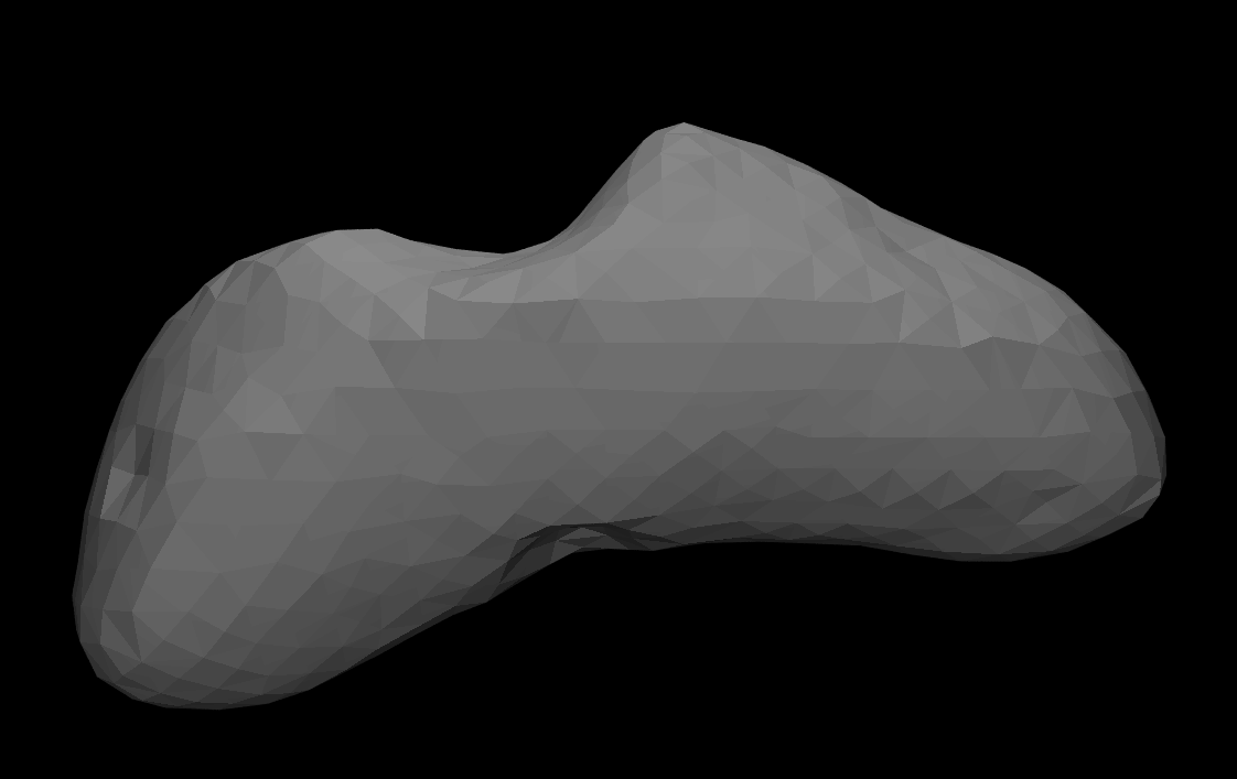
Figure 1: Depiction of the Eros shape model by Thomas2002 used by us. The figure was created using the freeware ray-tracing software POV-ray.

Our thermophysical modeling is based on the model of Eros’ shape and spin state by Thomas2002, the version with 1708 triangular facets is used (see Fig. 1). To validate our numerical treatment of the model geometry, we have in a first step attempted to reproduce published optical lightcurves of Eros, finding excellent agreement between synthetic optical lightcurves and published observational data by Hicks1999 and Erikson2000.

N-band data are analyzed which were obtained by HarrisDavies on June 27–30 1998 using the United Kingdom Infrared Telescope UKIRT on Mauna Kea / Hawai’i with the CSG3 spectrometer (see HarrisDavies, for details). There is a total of 7 spectra, each providing simultaneous photometry at 25 wavelengths between 8.06 and $13.04\text{\,}\mathrm{\SIUnitSymbolMicro m}$. While HarrisDavies referred all data to a common observing geometry and to the flux level of lightcurve average, we rather aim at reproducing each spectrum at the time of observation with the corresponding observing geometry. To this end, our TPM (see chapter 3) is used.

Most required input parameters have been determined from NEAR-Shoemaker results (Domingue2002; Thomas2002): $H=10.82$ as implied by $D=$16.9\text{\,}\mathrm{km}$$ and $p_{\text{V}}{}=0.29$, while the $p_{\text{V}}{}$-value and the reported Bond albedo imply $G=0.181$ (see eqn. 2 on p. 2). The J2000 ecliptic coordinates of the spin axis are $\beta=$+11.35\text{\,}\mathrm{\SIUnitSymbolDegree}$$, $\lambda=$17.22\text{\,}\mathrm{\SIUnitSymbolDegree}$$, implying a subsolar latitude at the time of the UKIRT observations of $+34\text{\,}\mathrm{\SIUnitSymbolDegree}$, a sub-Earth latitude of , and an hour angle of the Sun at the sub-Earth point of $+0.9\text{\,}\mathrm{h}$ corresponding to a “local time” of $12.9\text{\,}\mathrm{h}$, i.e. the afternoon side was observed.

3 Results

Figure 2: Eros: Reduced $\chi^{2}$ as a function of thermal inertia for different roughness parameters. With $7\times 25$ data points and two fit parameters (diameter and thermal inertia), the reduced $\chi^{2}$ equals $\chi^{2}/173$.

Figure 3: Eros: Best-fit diameter as a function of thermal inertia for different roughness parameters.

See Figures 2 and 3 for plots of the best-fit $\chi^{2}$ and diameters as a function of thermal inertia, using the methods detailed in sect. 5. Both figures contain slight “wiggly” artefacts for large thermal-inertia values due to the approximation mentioned therein; these artefacts quickly become unnoticeable with decreasing thermal inertia. The respective scale factor, $\kappa$, is closely related to the derivative of the curves given in Fig. 3, which are seen to be relatively flat; it has been verified that $\kappa$ is within $1\text{\,}\%$ of unity for all but the lowest and largest thermal-inertia values considered. To increase the numerical accuracy at low thermal inertia, one may decrease the step size in thermal inertia.

As apparent from Fig. 2, the best-fit thermal inertia is dependent on the assumed roughness parameters, where increasing roughness decreases the best-fit thermal inertia. The data are best fit for intermediate roughness parameters, roughly in the range of 100–$200\text{\,}\mathrm{J}\usk\power{\mathrm{s}}{-1/2}\power{\mathrm{K}}{-1}\power{\mathrm{m}}{-2}$ in thermal inertia.

As can be seen in Fig. 3, the best-fit diameter for low roughness and a thermal inertia of $150\text{\,}\mathrm{J}\usk\power{\mathrm{s}}{-1/2}\power{\mathrm{K}}{-1}\power{\mathrm{m}}{-2}$ (the best-fit value for these roughness parameters) is around $18.3\text{\,}\mathrm{km}$, while for default roughness the best-fit diameter is .

4 Discussion

The best-fit diameter is slightly model dependent, but within the range $17.8\pm$0.5\text{\,}\mathrm{km}$$, where the quoted uncertainty reflects solely the statistical scatter inherent in the data and the systematic uncertainty from the unknown roughness parameters. Other sources of uncertainty, which are hard to estimate a priori but are probably dominated by systematic modeling uncertainties, add to the error budget. The NEAR-Shoemaker result is $16.9\text{\,}\mathrm{km}$ (Thomas2002), some $5\text{\,}\%$ below our result.

The best-fit thermal inertia is 100–$200\text{\,}\mathrm{J}\usk\power{\mathrm{s}}{-1/2}\power{\mathrm{K}}{-1}\power{\mathrm{m}}{-2}$, in excellent agreement with previous estimates by LebofskyRieke1979 (140–$280\text{\,}\mathrm{J}\usk\power{\mathrm{s}}{-1/2}\power{\mathrm{K}}{-1}\power{\mathrm{m}}{-2}$) and HarrisDavies (). We reckon that our result supersedes previous estimates since it makes explicit use of Eros’ spin state and shape model determined from the NEAR-Shoemaker spacecraft.

Eros’ thermal inertia is more than an order of magnitude below that of bare rock and roughly three times the lunar value (see table 1 on p. 1), a very plausible value given spacecraft imaging of Eros’ surface, which reveal a regolith-dominated surface with a moderate amount of craters and boulders (Thomas2002); the latter being consistent with the higher-than-lunar thermal inertia.

We conclude that applying our TPM, based on a detailed shape model, to published thermal-infrared data of Eros results in estimates for diameter and thermal inertia which are in excellent agreement with previous estimates including “ground truth” from spacecraft observations. In particular, the diameter uncertainty due to systematic modeling uncertainties does not appear to vastly exceed $5\text{\,}\%$ for the favorable circumstances (large data set, accurate model of shape and spin state, moderate solar phase angle of $29\text{\,}\mathrm{\SIUnitSymbolDegree}$) of this study. No such studies for an NEA have been published before.

Eros’ shape model by Thomas2002 is not convex but contains several prominent concavities (see Fig. 1 on p. 1). Nevertheless, the convex-shape TPM produces results in excellent agreement with independently obtained results. This is somewhat unexpected because the indentations present on Eros’ surface would be expected to lead to shadowing effects and to mutual heating of surface elements as discussed in chapter LABEL:chapt:TPMconcave in the appendix. We conclude that neglecting the effects of non-convex global shape does apparently not lead to a critical systematic diameter offset for objects as irregularly shaped as Eros.

In general, neglecting shadowing leads to an overestimation of thermal flux and consequently to a diameter underestimation; the converse applies to neglecting mutual heating. The fact that our derived diameter is slightly larger than the spacecraft result may indicate that at the moderate phase angle of the considered observations () the effect of mutual heating dominates the cooling effect of shadowing, which may become more relevant at larger phase angles. Further analysis using a more general TPM accounting for shadowing and mutual heating are required to study this speculation.

We would expect more accurate constraints on Eros’ physical properties to result from a TPM fit to all thermal-infrared data available in the literature, including the flux values quoted in LebofskyRieke1979, such that the database would stretch a broader range in solar phase angle and aspect geometry. Note that, in contrast to simple models, our model can be used to consistently fit data obtained at different epochs. However, combining data obtained by different observers using different instruments requires a very careful assessment of potential cross-calibration issues and of the relative accuracies of the data sets, which is beyond our current scope.

5 Summary

In order to validate our TPM for application to NEAs, thermal-infrared observations (HarrisDavies) of the NEA (433) Eros have been reanalyzed. Eros had been scrutinized from ground and through the NEAR-Shoemaker spacecraft.

Eros’ diameter is reproduced to within of the NEAR-Shoemaker result (Thomas2002). The best-fit thermal inertia is 100–$200\text{\,}\mathrm{J}\usk\power{\mathrm{s}}{-1/2}\power{\mathrm{K}}{-1}\power{\mathrm{m}}{-2}$ depending on the assumed model roughness parameters, in excellent agreement with earlier estimates. Eros’ thermal inertia is more than an order of magnitude below that of bare rock and roughly three times the lunar value, a very plausible value given Eros’ surface structure as revealed by spacecraft imaging.

We conclude that our convex-shape TPM is well suited to analyze thermal-infrared observations of NEAs and to derive quantitative estimates of their diameter, albedo, and thermal inertia.

2 (25143) Itokawa

In 2005, the Japanese spacecraft Hayabusa has rendezvoused with the NEA (25143) Itokawa. Prior to that, in 2004, we had performed thermal-infrared observations of Itokawa with the IRTF and MIRSI, which are presented here. Preliminary results have been accepted for publication in the proceedings of the 1st Hayabusa symposium (Ito1), which has not yet been printed, however.

Additional thermal-infrared observations were published by MuellerItokawa, also before the arrival of Hayabusa. There included is a recalibration of other data points found in the literature, which he had used in our preliminary analysis.

We here present TPM analyses of different combinations of thermal-infrared data sets, including the first analysis of the complete set of reliable thermal data of Itokawa. The resulting best-fit diameter is 0.32–$0.33\text{\,}\mathrm{km}$, in excellent agreement with Hayabusa results. Together with the results of our Eros study (see sect. 1), this suggests that the systematic diameter uncertainty inherent in our thermophysical modeling does not exceed $10\text{\,}\%$.

Itokawa’s thermal inertia is found to be $700\pm$100\text{\,}\mathrm{J}\usk\power{\mathrm{s}}{-1/2}\power{\mathrm{K}}{-1}\power{\mathrm{m}}{-2}$$, refining the estimate by MuellerItokawa, $750\pm$250\text{\,}\mathrm{J}\usk\power{\mathrm{s}}{-1/2}\power{\mathrm{K}}{-1}\power{\mathrm{m}}{-2}$$.

1 Introduction

(25143) Itokawa (previously known as 1998 SF36) is an S-type NEA which is a particularly favorable spacecraft target due to the relatively moderate amount of energy and time required to reach it. It has been studied in detail from the spacecraft Hayabusa during a rendezvous in 2005 (see Fujiwara2006, and references therein). Apart from a detailed study of the asteroid’s physical properties using remote sensing techniques while hovering within a few kilometers of the asteroid surface, Hayabusa was scheduled to take small samples of asteroid material and to return them to Earth. Due to technical problems it is currently unclear whether Hayabusa has succeeded in taking samples and whether it will manage to return to Earth; the planned Earth-arrival date is in 2010.

We have observed Itokawa at the IRTF in July 2004, before the arrival of Hayabusa at its target. Apogee data obtained by us have been used by KaasalainenIto in the derivation of Itokawa’s shape and spin state. Our MIRSI data, combined with other data found in the literature, have been used by us to determine Itokawa’s size and thermal inertia.

A vast body of information on Itokawa has been collected both before and after the arrival of Hayabusa using different techniques, we here focus on those which are most relevant for our purposes, i.e. estimates of size, shape, and thermal inertia.

Pre-Hayabusa

Sekiguchi2003 report single-wavelength N-band photometry and estimate the diameter of Itokawa to be , using the STM (see sect. 1). Combining the Sekiguchi2003 flux measurement with newly obtained $\text{M}^{\prime}$-band photometry at $4.68\text{\,}\mathrm{\SIUnitSymbolMicro m}$, Ishiguro2003 derive dimensions for a triaxial ellipsoid of $(620\pm 140)\times(280\pm 60)\times(160\pm 30)$ m , corresponding to an effective diameter of roughly . Ishiguro2003 also report a thermal inertia of $290\text{\,}\mathrm{J}\usk\power{\mathrm{s}}{-1/2}\power{\mathrm{K}}{-1}\power{\mathrm{m}}{-2}$, which they derive from the two thermal-infrared data points at their disposal. Their thermal model assumes a spherical shape.

From radar observations, Ostro2004 determine a shape model of Itokawa and a volume-equivalent diameter of . After obtaining new radar observations in June 2004, Ostro2005 publish an updated shape model and size estimate, with ellipsoidal axes within $10\text{\,}\%$ of $594\times 320\times 288$  m , corresponding to a volume-equivalent diameter of .

KaasalainenIto determined the spin state of Itokawa and a convex-definite model of its shape from the inversion of optical lightcurve data.

From a preliminary analysis of the thermal-infrared data published by Sekiguchi2003 and Ishiguro2003, and new data which had been obtained at the ESO 3.6-m telescope (later published in Delbo2004) and at the IRTF (see below), we (Ito1) determined a diameter around $280\text{\,}\mathrm{m}$ and a thermal inertia of some $350\text{\,}\mathrm{J}\usk\power{\mathrm{s}}{-1/2}\power{\mathrm{K}}{-1}\power{\mathrm{m}}{-2}$. Our analysis was based on the KaasalainenIto shape model and the TPM described in chapter 3. The thermal-inertia result is intermediate between lunar regolith and bare rock (but closer to the former) and was interpreted as “incompatible with a surface dominated by bare rock.” An Eros-like surface was proposed but with a coarser regolith and/or a larger number of boulders.

MuellerItokawa obtained further thermal-infrared flux measurements at the ESO 3.6-m telescope. Combining their data with those of Sekiguchi2003 and Delbo2004 but with neither our MIRSI data (which were not available to them) nor the Ishiguro2003 M-band value, they determined a diameter of and a thermal inertia of $750\text{\,}\mathrm{J}\usk\power{\mathrm{s}}{-1/2}\power{\mathrm{K}}{-1}\power{\mathrm{m}}{-2}$, which they interpret as “an indication for a bare rock dominated surface.” Their results are based on the thermophysical model by LagerrosI; LagerrosIII; LagerrosIV and the shape model by KaasalainenIto which had also been used by us.

Table 1: Itokawa: Overview of published diameter estimates, $D$, and reported uncertainties, $\sigma$.

$D(\mathrm{k}\mathrm{m})$	$\sigma(\mathrm{k}\mathrm{m})$	Source
0.35	0.03	Sekiguchi2003
0.30	0.03	Ishiguro2003
0.36	0.04	Ostro2004
0.38	0.04	Ostro2005
0.28	—	Ito1
0.32	0.03	MuellerItokawa
0.327	0.006	Demura2006

Hayabusa results

From Hayabusa observations, Demura2006 determined a volume within $5\text{\,}\%$ of $0.018378\text{\,}{\mathrm{km}}^{3}$, corresponding to a volume-equivalent diameter of (see eqn. 1). See table 1 for an overview of published diameter estimates.

Demura2006 also report an updated shape model which appears to be in broad agreement with that by KaasalainenIto, however at the time of writing it has not yet been released to the scientific community. A spin axis is reported within $3.9\text{\,}\mathrm{\SIUnitSymbolDegree}$ of $\lambda=$128.5\text{\,}\mathrm{\SIUnitSymbolDegree}$$ and $\beta=$-89.66\text{\,}\mathrm{\SIUnitSymbolDegree}$$ (J2000 ecliptic coordinates), in very good agreement with the estimate by KaasalainenIto.

From global imaging of Itokawa (see, e.g., Fig. 1 on p. 1) one recognizes a dichotomy between rough and smooth terrains on Itokawa’s surface, which cover some 80 and $20\text{\,}\%$ of the surface area, respectively (Saito2006). Rough terrains are densely covered in boulders of various sizes, in contrast to smooth areas which display very low boulder abundance.

During operations in preparation of the spacecraft touchdowns for sample taking and during the two touchdowns themselves, high-resolution imaging was obtained of the vicinity of the touchdown sites, i.e. of parts of the Muses-C region and of adjacent rough terrain (Yano2006). The obtained images of smooth terrain display a dense cover of coarse regolith consisting of gravel in the m m – c m  range with no apparent sign of finer dust on the surface. Itokawa’s regolith is coarser than the regolith found in Eros’ ponds (Yano2006). The smooth regolith-covered regions were found to coincide with the minima of the gravitational potential (see Fujiwara2006). Based on an analysis of high-resolution imaging, Miyamoto2007 report evidence for “landslide-like granular migration” on Itokawa’s surface, i.e. for regolith migration aligned with the local gravity slope. They conclude that Itokawa’s surface is unconsolidated and suggest that vibrations due to, e.g., impact-induced seismic shaking cause gravel fluidization and subsequent down-slope movement, where the resulting grain mobility increases with decreasing grain size.

A very low abundance of crater-like features was found on Itokawa’s surface, totaling no more than 100 for crater diameters exceeding $70\text{\,}\mathrm{cm}$ (see Saito2006). Craters of small and intermediate size may be buried in migrating regolith; Miyamoto2007 present images of regolith concentrations on the floors of crater-like features.

One estimate of a local value of thermal inertia is available, obtained from an indirect temperature measurement during touchdown. The temperature close to the sampling site in the Muses-C terrain is estimated by Yano2006 to be , which they conclude is indicative of a thermal inertia in the range between 100 and $1000\text{\,}\mathrm{J}\usk\power{\mathrm{s}}{-1/2}\power{\mathrm{K}}{-1}\power{\mathrm{m}}{-2}$, although there appear to be significant systematic uncertainties in their thermal modeling.

2 Thermal-infrared observations

We have observed Itokawa with the NASA IRTF (see chapter 4) on Mauna Kea / Hawai’i using MIRSI and Apogee on 10 July 2004 (UT). The Apogee data are not needed here, hence they shall be disregarded in the following. Additional observations were scheduled for 28 and 29 July but failed due to bad weather. The night of 10 July was photometric but had a relatively high (constant) level of atmospheric humidity.

During our observations, Itokawa’s heliocentric distance was , its topocentric distance from Mauna Kea was , the solar phase angle was $28.3\text{\,}\mathrm{\SIUnitSymbolDegree}$. Itokawa’s declination was , the airmass at meridian transit ($\sim$ 12:15 UT) was 2.0. Unfortunately, technical problems disabled MIRSI observations for some 90 minutes around transit, hence the reported MIRSI observations have been obtained at larger airmasses. The CohenVII; CohenX calibration standard stars $\beta$ And and $\alpha$ Lyr have been observed at similarly large airmasses before and after the Itokawa observations. MIRSI data have been reduced using the methods described in sect. 4; see table 2 for the resulting flux values.

Table 2: Flux values resulting from MIRSI observations of Itokawa on 10 July 2004 (UT). Times given refer to the middle of the exposure and are corrected for 1-way light-time.

Time	Wavelength	Flux	$\sigma$ flux
( h )	( µ m )	$\left[\frac{10^{-15}\mathrm{W}}{\mathrm{m}^{2}\mathrm{\SIUnitSymbolMicro}\mathrm{m}}\right]$	$\left[\frac{10^{-15}\mathrm{W}}{\mathrm{m}^{2}\mathrm{\SIUnitSymbolMicro}\mathrm{m}}\right]$
11.73888	11.7	16.7	2.2
11.79576	11.7	15.8	2.0
13.52352	11.7	20.0	2.5
13.67784	9.8	24.7	3.9
13.84128	9.8	17.8	3.8

In Ito1, preliminary TPM fits are reported based on the MIRSI data quoted in table 2, thermal fluxes obtained at the ESO 3.6-m telescope with TIMMI2 on 8 April 2001 (Delbo2004, measurements from 9 April are also reported but were not used due to the reported unfavorable atmospheric conditions in that night), and respectively one thermal flux value from Sekiguchi2003 and Ishiguro2003. Later, we were informed that the $4.68\text{\,}\mathrm{\SIUnitSymbolMicro m}$ flux value reported by Ishiguro2003 was likely to be compromised (Hasegawa, 2004, private communication; Hasegawa is a co-author of that paper).

The database of MuellerItokawa contains new TIMMI2 measurements in addition to those used by us (Delbo2004 and Sekiguchi2003). Our MIRSI data were not available to them. They chose not to use the $4.68\text{\,}\mathrm{\SIUnitSymbolMicro m}$ flux by Ishiguro2003 Flux values originally reported by Delbo2004 and Sekiguchi2003 have been recalibrated by MuellerItokawa

We have used our TPM described in chapter 3 to fit different combinations of data sets. Itokawa’s absolute optical magnitude is assumed to be $H=19.5$ throughout our analysis, which appears to be consistent with our Apogee data. The exact choice of $H$ would be expected to have negligible influence on diameter and thermal-inertia results. The following data sets are analyzed:

1. That considered in Ito1, i.e. MIRSI data, TIMMI2 data by Delbo’ (8 April 2001) + Sekiguchi2003, and M-band data by Ishiguro2003 Unlike in Ito1, recalibrated TIMMI2 fluxes are used. (total: 12 data points)

2. As above, but without the Ishiguro2003 M-band data: MIRSI + recalibrated TIMMI2 data by Delbo’ and Sekiguchi2003 (total: 11 data points)

3. The “high-quality” data points reported in MuellerItokawa, including Delbo2004 and Sekiguchi2003 data as above. (total: 15 data points)

4. All reliable data, i.e. the 15 data points as above in addition to our MIRSI data. (total: 20 data points)

3 Results

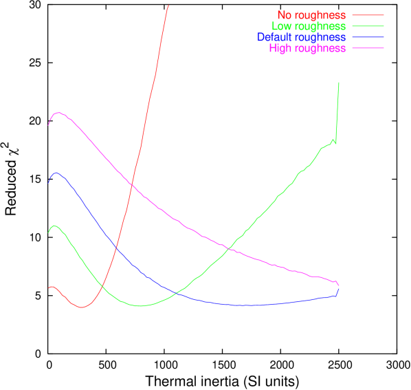
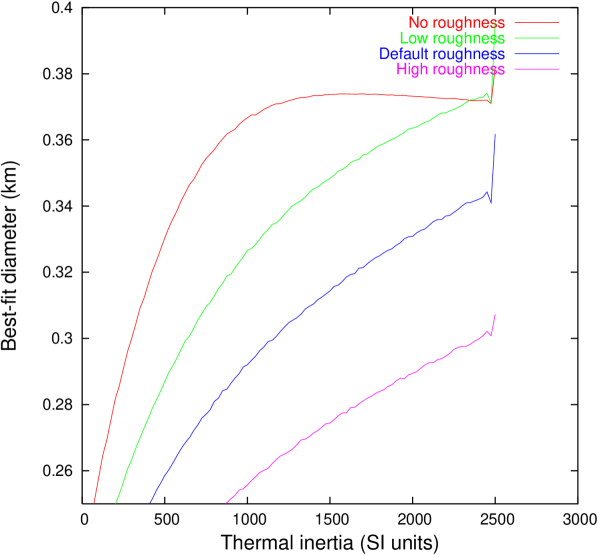
Figure 4: Itokawa: TPM fits to data set 1, i.e. the flux values considered in Ito1. Left: Reduced $\chi^{2}$ as a function of thermal inertia for four sets of roughness parameters (see sect. 5). Right: Best-fit diameter as a function of thermal inertia.

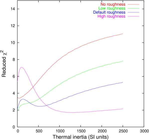
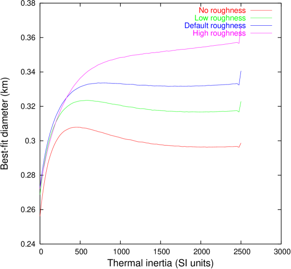
Figure 5: As Fig. 4, but without the $4.68\text{\,}\mathrm{\SIUnitSymbolMicro m}$ flux value reported by Ishiguro2003 (data set 2).

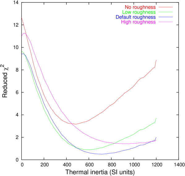
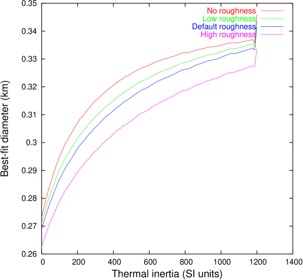
Figure 6: As Fig. 4, but for the data set quoted by MuellerItokawa (data set 3).

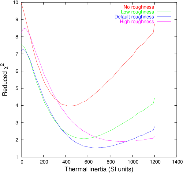
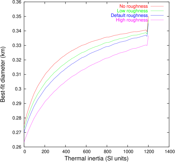
Figure 7: As Fig. 4, but for the complete set of reliable thermal-infrared data, i.e. those quoted by MuellerItokawa in addition to the MIRSI data given in table 2 (data set 4).

See Figures 4, 5, 6, and 7 for our model analyses of the four data sets described above. See sect. 1 for a detailed discussion of analogous plots and their interpretation. Our results for the individual data sets are:

1. Depending on roughness parameters, $\chi^{2}$ is minimized at very different thermal-inertia values. Thermal inertia is not well constrained by the data, although values much below $250\text{\,}\mathrm{J}\usk\power{\mathrm{s}}{-1/2}\power{\mathrm{K}}{-1}\power{\mathrm{m}}{-2}$ would appear to be inconsistent. The corresponding best-fit diameters vary between $296\text{\,}\mathrm{m}$ (no roughness, $\Gamma=$275\text{\,}\mathrm{J}\usk\power{\mathrm{s}}{-1/2}\power{\mathrm{K}}{-1}\power{\mathrm{m}}{-2}$$) and $319\text{\,}\mathrm{m}$ (default roughness, $\Gamma=$1650\text{\,}\mathrm{J}\usk\power{\mathrm{s}}{-1/2}\power{\mathrm{K}}{-1}\power{\mathrm{m}}{-2}$$). The difference in best-fit diameter when compared to Ito1 is due to the recalibration of the ESO fluxes discussed above. Fitting the data for individual sets of roughness parameters clearly shows that there is no well constrained global $\chi^{2}$ minimum. This was somewhat obscured by the approach used in Ito1, where crater density was used as a variable fit parameter.

2. Thermal inertia is unconstrained within the range 0–$2500\text{\,}\mathrm{J}\usk\power{\mathrm{s}}{-1/2}\power{\mathrm{K}}{-1}\power{\mathrm{m}}{-2}$, the largest value considered in our analysis (thermal inertia of bare rock). Zero roughness appears to be a poor fit to the data, but none of the remaining three roughness models is excluded. The corresponding best-fit diameters vary between 0.27 and $0.35\text{\,}\mathrm{km}$. Note that by disregarding a single data point we could significantly improve the quality of the fit: the reduced $\chi^{2}$ now reaches much lower values than for data set 1.

3. There is a clear global minimum for “default” roughness at thermal-inertia values between 600 and $800\text{\,}\mathrm{J}\usk\power{\mathrm{s}}{-1/2}\power{\mathrm{K}}{-1}\power{\mathrm{m}}{-2}$, although slightly lower values ($\Gamma$ between 500 and $700\text{\,}\mathrm{J}\usk\power{\mathrm{s}}{-1/2}\power{\mathrm{K}}{-1}\power{\mathrm{m}}{-2}$) and “low” roughness are not ruled out. Zero and “high” roughness would appear to be less consistent with the data. For the quoted ranges in thermal inertia, the corresponding best-fit diameters vary between 0.320 and $0.326\text{\,}\mathrm{km}$.

4. The global minimum for “default” roughness and thermal inertia between 600 and $800\text{\,}\mathrm{J}\usk\power{\mathrm{s}}{-1/2}\power{\mathrm{K}}{-1}\power{\mathrm{m}}{-2}$ remains, “low” roughness is less well consistent with the data than before. The corresponding best-fit diameters vary between 0.323 and $0.329\text{\,}\mathrm{km}$.

These results are summarized in table 3.

Table 3: Itokawa: Results of TPM fits to the four data sets considered (see Figs. 4–7).

Data set	Diameter	Thermal inertia
	( m )	( J s -1/2 K -1 m -2)
1	296–319	$\geq 250$
2	270–350	0–2500
3	320–326	500–800
4	323–329	600–800

4 Discussion

Diameter

Taken at face value, the best-fit diameter resulting from our TPM analysis of all available reliable thermal-infrared data is $326\pm$3\text{\,}\mathrm{m}$$, in amazingly good agreement with the Hayabusa result of $327\pm$6\text{\,}\mathrm{m}$$ (Demura2006). We caution, however, that solely the scatter in the flux values is reflected in the quoted range of uncertainty. Systematic flux calibration uncertainties and systematic uncertainties inherent in our TPM and in the shape model add to the error budget. Nevertheless, this close match emphasizes the potentially very high accuracy of diameter estimates derived from TPM analysis of a suitable thermal-infrared database. Combining this with results from an analysis of Eros data (see also sect. 1), where we were able to reproduce the diameter estimate derived from spacecraft measurements to within , we conclude that $10\text{\,}\%$ is a conservative upper limit on the systematic diameter uncertainty inherent in our thermophysical modeling (see sect. LABEL:sect:NEA:D), resulting in a final diameter result of $0.32\pm$0.03\text{\,}\mathrm{km}$$.

We note that our preliminary results reported in Ito1 were plagued by inaccuracies in flux values quoted from other sources. Using recalibrated TIMMI2 flux values resolves the diameter discrepancy between our preliminary analysis ($D\sim$0.28\text{\,}\mathrm{km}$$) and the Hayabusa result, $0.327\pm$0.006\text{\,}\mathrm{km}$$ rejecting the unreliable (Hasegawa, 2004, private communication) M-band flux by Ishiguro2003 significantly increased the goodness of fit.

Thermal inertia

The best-fit thermal inertia is $700\pm$100\text{\,}\mathrm{J}\usk\power{\mathrm{s}}{-1/2}\power{\mathrm{K}}{-1}\power{\mathrm{m}}{-2}$$. This refines the estimate by MuellerItokawa, which was based on a subset of the database available to us. A reanalysis of their data set confirms their result.

The TPM-derived thermal-inertia result is significantly larger than the estimate by Ishiguro2003 of . This is not entirely surprising given the small data set of only two thermal-infrared data points available to them. Furthermore, Ishiguro2003 analyzed their data using a simplistic thermal model based on spherical geometry which we would expect to be inappropriate for a quantitative determination of thermal inertia.

Geological interpretation of thermal inertia in the light of Hayabusa results

A thermal inertia of $700\pm$100\text{\,}\mathrm{J}\usk\power{\mathrm{s}}{-1/2}\power{\mathrm{K}}{-1}\power{\mathrm{m}}{-2}$$ corresponds to some 14 times the lunar value, so Itokawa’s surface would not be expected to be dominated by fine Moon-like regolith. On the other hand, $700\text{\,}\mathrm{J}\usk\power{\mathrm{s}}{-1/2}\power{\mathrm{K}}{-1}\power{\mathrm{m}}{-2}$ is less than a third of the thermal inertia of solid rock (see table 1 on p. 1). As highlighted by MuellerItokawa, Itokawa’s corresponding thermal conductivity is $\kappa\sim$0.3\text{\,}\mathrm{W}\usk\power{\mathrm{K}}{-1}\power{\mathrm{m}}{-1}$$ which they conclude is a plausible value for “porous stony material”. As can be seen from table 1, an extremely large porosity would be required to explain this conductivity: 0.3 is smaller than the value for solid rock by a factor of ten, and only twice as large as the value for the very vesicular material pumice, which is an implausible model for asteroidal “bare rock”.

Among the materials listed in table 1, the best matches to Itokawa’s thermal inertia are compact snow, sandy soil, and coal. Given Itokawa’s taxonomic classification as S type, sandy soil would be expected to be the best analogue, although we caution that the atmosphere (and furthermore humidity inside the soil) skew thermal-inertia values measured on Earth towards larger values relative to asteroid surfaces.

We note that the thermal skin depth (eqn. 10a on p. 10a), i.e. the length scale for the penetration of the diurnal heat wave, is of the order of several centimeters given our thermal-inertia result. Gravel with grain sizes up to some $10\text{\,}\mathrm{cm}$ would therefore be expected to display a reduced thermal inertia relative to boulders made of the same material. Furthermore, a dust coating (thin compared to the skin depth) would reduce the thermal inertia of a boulder. This will be further discussed in sect. LABEL:sect:NEA:barerock.

Based on Hayabusa measurements obtained while descending to a sampling site in smooth terrain, a local thermal-inertia value between 100 and $1000\text{\,}\mathrm{J}\usk\power{\mathrm{s}}{-1/2}\power{\mathrm{K}}{-1}\power{\mathrm{m}}{-2}$ was obtained (Yano2006). The sampling site was seen from close-up imaging to be covered with coarse regolith, with typical grain sizes in the m m – c m  range. It is reasonable to expect the sampling site to be representative of Itokawa’s smooth terrains, which cover some $20\text{\,}\%$ of the total area (see Saito2006). For the rough terrains, which cover some $80\text{\,}\%$ of the surface area, no local thermal-inertia measurement is available. A small fraction of the rough terrain, adjacent to the touchdown site in the smooth Muses-C region, was imaged in high resolution; the images reported by Miyamoto2007 show much larger grain sizes than in smooth terrain. While particle sizes for the rough terrain are not explicitly reported by Miyamoto2007, their Fig. 2c appears to display a very low abundance of pebble-sized gravel but rather appears to be dominated by larger cobbles which are comparable to the thermal skin depth (centimeters) in size.

From our global thermal-inertia result it appears that the typical thermal inertia on Itokawa’s surface does not greatly exceed that of the sampling site, although we caution that the latter is only poorly constrained so far. We speculate that the large boulders apparent in Hayabusa imaging of the rough terrain (see, e.g., Saito2006, Figs. 3 and 4) are covered with a thin dust coating. Alternatively, the “bare rock” of which Itokawa’s boulders are composed may be a poor thermal conductor relative to granite found on Earth; this could be caused by, e.g., a high amount of porosity at length scales smaller than the skin depth, i.e. at the m m -scale or smaller. Note that Christensen2003 report a thermal inertia up to $2200\text{\,}\mathrm{J}\usk\power{\mathrm{s}}{-1/2}\power{\mathrm{K}}{-1}\power{\mathrm{m}}{-2}$ for outcrops of exposed bedrock on Mars (the floor of the Nili Patera caldera).

We wish to stress that the dependence of thermal inertia on grain size, which is well established for the atmospheric pressures prevalent on Earth (see Clauser1995) and Mars (see Presley1997), is significantly less well studied in a vacuum. Laboratory measurements of the thermal inertia of particulate materials in a vacuum chamber would be very valuable for the interpretation of our results. The same applies to the effect of porosity on thermal inertia—note that the residual atmospheric gas inside pores enhances the thermal conductivity and hence the thermal inertia.

Mutual consistency of thermophysical models

The data set of 15 flux values considered by MuellerItokawa to be of “high quality” has been reanalyzed. While MuellerItokawa used the TPM by LagerrosI; LagerrosIII; LagerrosIV in their analysis, we use that described in chapter 3 which is largely based on Lagerros’ but has been implemented independently.

They report $D=0.32\pm$0.03\text{\,}\mathrm{km}$$ and $\Gamma=$750\text{\,}\mathrm{J}\usk\power{\mathrm{s}}{-1/2}\power{\mathrm{K}}{-1}\power{\mathrm{m}}{-2}$$. No formal thermal-inertia uncertainty is given, but values between 500 and $1000\text{\,}\mathrm{J}\usk\power{\mathrm{s}}{-1/2}\power{\mathrm{K}}{-1}\power{\mathrm{m}}{-2}$ are reported to be consistent with their data. Both results are largely reproduced in our reanalysis. Comparing their Fig. 4 with the “default roughness” curve in Fig. 6 on p. 6, it appears that our result is slightly skewed towards lower thermal inertia. This may be due to the different fitting techniques used (MuellerItokawa do not attempt to minimize $\chi^{2}$ but rather the fractional formal diameter uncertainty, which is not entirely equivalent) and does not lead to significantly different results.

We conclude that the TPM by LagerrosI; LagerrosIII; LagerrosIV and that described herein are mutually consistent.

5 Summary

A TPM analysis of all available thermal-infrared data of the NEA (25143) Itokawa, the target of the Japanese mission Hayabusa, results in a diameter estimate between 320 and $330\text{\,}\mathrm{m}$, in excellent agreement with the Hayabusa result of $327\pm$6\text{\,}\mathrm{m}$$. Combining this with the results of our Eros study (see sect. 1) we conclude that $10\text{\,}\%$ is a conservative upper limit on the systematic diameter uncertainty inherent in our thermophysical modeling.

We find Itokawa’s thermal inertia to be $700\pm$100\text{\,}\mathrm{J}\usk\power{\mathrm{s}}{-1/2}\power{\mathrm{K}}{-1}\power{\mathrm{m}}{-2}$$, thus refining the estimate by MuellerItokawa, which is based on a subset of the data available to us. A reanalysis of their database reproduces their results, thus demonstrating the mutual consistency of our TPM and that by LagerrosI; LagerrosIII; LagerrosIV which was used by MuellerItokawa

Itokawa’s thermal inertia is intermediate between that of bare rock and dusty regolith. This is not straightforward to reconcile with Hayabusa close-up imaging results, which reveal a surface dominated by relatively large boulders. We speculate that boulders on Itokawa are covered with a thin coating of dust. This will be further discussed in sect. LABEL:sect:NEA:barerock. We call for a reanalysis of the thermal-infrared database using the accurate Hayabusa-derived shape model, which has been released to the scientific community on 24 April 2007.

3 (1580) Betulia

The C-type NEA (1580) Betulia is a highly unusual object for which earlier radiometric observations, interpreted on the basis of simple thermal models, indicated a surface of unusually high thermal inertia (see sect. 1).

We report results from extensive multi-wavelength thermal-infrared observations of Betulia obtained in 2002 with the NASA Infrared Telescope Facility IRTF. From a TPM analysis we determine that Betulia’s thermal inertia is only moderate, around $180\text{\,}\mathrm{J}\usk\power{\mathrm{s}}{-1/2}\power{\mathrm{K}}{-1}\power{\mathrm{m}}{-2}$, comparable to our other NEA results. We determine an effective diameter of and an albedo of $p_{\text{V}}{}=0.077\pm 0.015$, consistent with expectations based on the taxonomic type. Our results are in broad agreement with an independent NEATM analysis of the same data set but are hard to reconcile with previous results with indicate a much larger diameter and, indirectly, a high thermal inertia indicative of bare rock.

After publication, our diameter and albedo estimates have been confirmed on the basis of a reanalysis of available polarimetric data and, independently, on the basis of new radar observations.

1 Introduction

The C-type NEA (1580) Betulia is well known for its unusual lightcurve, the amplitude and form of which changes dramatically with changing solar phase angle; particularly, at large phase angles it exhibits a triply-peaked lightcurve as opposed to the doubly-peaked lightcurves of virtually all other asteroids (TedescoBetulia). These and other lightcurve data were used by KaasalainenBetulia to determine Betulia’s spin state and a convex-definite model of its shape. They found the shape to be “very peculiar with a large planar area on one side” which they note may conceal a considerable concavity (their method of shape determination is designed to produce convex models). It is important to bear Betulia’s unusual shape in mind when interpreting observational data with the aid of standard photometric, polarimetric, and radiometric techniques.

Betulia is also significant in being the first NEA for which thermal-infrared observations indicated a surface of high thermal inertia (see sect. 1). LebofskyBetulia obtained thermal-infrared data at a single thermal wavelength ($10.6\text{\,}\mathrm{\SIUnitSymbolMicro m}$). Using the STM (see sect. 1), which neglects thermal inertia, they obtained a diameter of , inconsistent with a lower bound on the diameter of derived from radar observations (PettengillBetulia) and furthermore with polarimetric observations, which appeared to indicate a diameter around $7\text{\,}\mathrm{km}$ (TedescoBetulia). Because of this inconsistency, LebofskyBetulia rejected the STM diameter and used instead the FRM (see sect. 2), obtaining , concluding that Betulia had a very high thermal inertia, comparable to that of bare rock.

Betulia was observed extensively during an observing run with the NASA Infrared Telescope Facility (IRTF) in June 2002. Good quality data over a significant part of the rotation period were obtained at five wavelengths in the range 7–$20\text{\,}\mathrm{\SIUnitSymbolMicro m}$. We have fitted the resulting flux data with the TPM for convex shapes (see chapter 3) based on the shape model by KaasalainenBetulia.

2 Observations and data reduction

Table 4: Betulia: Observing geometry. Values for the subsolar and sub-Earth latitude are based on the spin axis by KaasalainenBetulia.

	2002 June 02	2002 June 05
Heliocentric distance, $r$ (AU)	1.143	1.150
Geocentric distance, $\Delta$ (AU)	0.246	0.263
Solar phase angle, $\alpha$ ( °)	52.9	53.3
Subsolar latitude ( °)	13	15
Sub-Earth latitude ( °)	-39	-34

The observations were performed on 2002 June 2 and June 5 UT with the IRTF and JPL’s $128\times 128$ pixel, 7–$25\text{\,}\mathrm{\SIUnitSymbolMicro m}$ infrared astronomical camera, MIRLIN. For details of MIRLIN see MIRLIN and http://cougar.jpl.nasa.gov/mirlin.html. Measurements were made in N-band filters centered at (bandwidth in brackets): 7.91 (0.76), 10.27 (1.01), and 11.7 (1.11)  µ m , and in Q-band filters at: 17.93 (0.45) and 20.81 (1.65)  µ m . See Betulia for details on the observations.

Standard synthetic aperture procedures (see sect. 4) were used for the derivation of raw signal counts from the MIRLIN images. Absolutely calibrated fluxes for the target asteroids were obtained by multiplying the integrated absolute fluxes of the calibration stars by the ratios of the target/calibration star raw counts in each filter. Absolutely calibrated infrared spectra for the calibration stars, $\alpha$ Boo and $\alpha$ Hya, were taken from the database of CohenX. Color corrections for the different flux distributions of the calibration stars and asteroids in the narrow filter pass bands were found to be no more than a few percent (Delbo2004) and were not applied.

Table 5: Betulia: Measured flux values

Date (UT)	Time	Julian date	Wavelength	Flux	Error
	(UT)	(days-2,452,420)	( µ m )	( m Jy)	( m Jy)
2002-06-02	05:59	7.7493	7.91	1400	57
	07:03	7.7937	7.91	1789	61
	08:09	7.8396	7.91	1803	67
	06:07	7.7549	10.27	2270	36
	07:11	7.7993	10.27	3334	32
	08:17	7.8451	10.27	3315	45
	06:16	7.7611	11.70	2347	38
	07:19	7.8049	11.70	3900	36
	08:24	7.8500	11.70	3166	37
	06:29	7.7701	17.93	4445	568
	07:33	7.8146	17.93	4745	311
	08:37	7.8590	17.93	4670	343
2002-06-05	05:50	10.7431	7.91	1150	67
	07:04	10.7944	7.91	1277	74
	08:13	10.8424	7.91	1302	84
	05:57	10.7479	10.27	2171	60
	07:11	10.7993	10.27	2364	74
	08:20	10.8472	10.27	1998	71
	06:02	10.7514	11.70	2606	38
	07:16	10.8028	11.70	2312	51
	08:25	10.8507	11.70	2458	39
	06:13	10.7590	17.93	2635	247
	07:25	10.8090	17.93	3406	247
	08:35	10.8576	17.93	2528	290
	06:28	10.7694	20.81	3235	177
	07:39	10.8187	20.81	2663	189
	08:47	10.8660	20.81	3172	176

Table 4 lists the observing geometry. The resulting fluxes are listed in table 5. The quoted uncertainties in the flux measurements refer to the formal statistical uncertainties in the synthetic aperture procedure, only. Errors in the absolute calibration and fluctuations in atmospheric conditions during the observations increase the scatter in the flux data. On 2002 June 2, an R-band (visible) lightcurve was obtained simultaneously with our IRTF observations on the University of Hawaii’s 88-inch telescope and kindly made available by Yan Fernández (2002, private communication).

3 Results

Figure 8: Betulia: Synthetic optical lightcurve using the shape model from KaasalainenBetulia for the observing geometry of 2002 June 2. There is very good agreement in shape and amplitude between the synthetic curve and the corresponding R-band measurements. The positioning of the synthetic lightcurve relative to the R-band measurements was adjusted manually on both axes to obtain a good fit, leading to a slight correction to the rotational period within the uncertainties quoted by KaasalainenBetulia (see text for details).

Our TPM analysis is based on the convex shape model by KaasalainenBetulia which consists of 3192 triangular facets. The corresponding spin axis is and (J2000 ecliptic latitude and longitude, respectively; from M. Kaasalainen, 2003, private communication). KaasalainenBetulia give a rotation period of on the basis of observations between the years 1976 and 1989. Using these parameters, we have generated a synthetic optical lightcurve for the observing geometry of 2002 June 2 and compared it to the R-band data by Fernández (see Fig. 8). We found a slight offset in rotational phase of around $29\text{\,}\mathrm{min}$ which was corrected for by adjusting the rotation period to a value of $6.1383602\text{\,}\mathrm{h}$, well within the quoted range of uncertainty.

Applying our TPM (see chapter 3) to the IRTF measurements listed in table 5, assuming $H=15.1$ and $G=0.15$ (see Betulia, and references therein), resulted in an effective diameter, $D_{\text{eff}}$, of , a geometric albedo, $p_{\text{V}}{}$, of $0.077\pm 0.005$, and a thermal inertia of . The quoted errors reflect only the statistical scatter about the model curve; modeling uncertainties are much larger than the formal errors. Comparison with independent results for $D_{\text{eff}}$ in the cases of (433) Eros and (25143) Itokawa suggests the uncertainty in diameter determinations with the TPM does not exceed $10\text{\,}\%$ (see sect. LABEL:sect:NEA:D).

Figure 9: Betulia: Comparison of synthetic N-band and synthetic optical lightcurves for the observing geometry of 2002 June 2. Points corresponding to the measured N-band fluxes are superimposed. For this plot, data obtained on June 5 are referred to June 2 by subtracting 12 rotational periods and by adjusting the flux values for the changes in observing geometry (whereby the dominant effect is due to the change in geocentric distance, see table 4). No manual adjustments to the N-band synthetic lightcurve or measurement points were made.

Figure 10: Betulia: Comparison of synthetic Q-band and synthetic optical lightcurves, points corresponding to the measured Q-band fluxes are superimposed as in Fig. 9. The plotted Q-band lightcurve results from parameters which best fit the total data set including N-band data.

There is evidence in Fig. 9 for a phase lag between the observed optical and thermal-infrared lightcurves which has the same sense and appears to be roughly the same fraction of the rotation period as that observed by LebofskyRieke1979 in the case of (433) Eros, which they explained in terms of surface thermal inertia (see also sect. 1). Given the differences in the structure of the optical and N-band synthetic lightcurves evident in a comparison of the two lightcurves over a full rotation period, the significance of the apparent small phase lag is not clear. The synthetic Q-band lightcurve (Fig. 10) does not display a clear phase lag. The resolution of this discrepancy may lie in shortcomings of the shape model and the TPM: for example, possible variations in albedo and thermal inertia over the surface are ignored, and treatment of the surface structure in the TPM is limited to an idealistic distribution of hemispherical craters. We have no satisfactory quantitative explanation for the discrepancy at present and further development of the model may be required to more accurately reproduce the details of the observations.

4 Discussion

Table 6: Betulia: Summary of diameter and albedo determinations. Values given in brackets were determined by us, assuming $H=15.1$, in order to facilitate comparison.

Source	$D_{\text{eff}}$ ( k m )	$p_{\text{V}}{}$
This work	$4.57\pm 0.46$	$0.077\pm 0.015$
TedescoBetulia, polarimetry	$\sim 7$	$\sim 0.033$
LebofskyBetulia, STM	$4.20\pm 0.80$	($0.091\pm 0.035$)
”, FRM	$7.48\pm 0.34$	($0.029\pm 0.003$)
PettengillBetulia, radar	$>5.4$	($<0.055$)
Betulia, NEATM	$3.82\pm 0.58$	$0.11\pm 0.04$
Tedesco (2005, private communication)	$4.76\pm 0.74$	$0.071\pm 0.005$
Magri2007, radar	$5.39\pm 0.54$	($0.055\pm 0.011$)

Diameter and albedo

See table 6 for a comparison of our diameter and albedo result with previous determinations. It is instructive to first compare our results with the NEATM results by Betulia, which are based on the same data set. While the TPM gives a somewhat larger diameter and lower albedo (the latter being more in line with expectations for a C-type asteroid) the two sets of results are in reasonable agreement given the uncertainties associated with both models, especially at the large solar phase angle at which our observations were made.

Our results are, however, inconsistent with the radar-derived lower limit on diameter of (PettengillBetulia) and with the polarimetric albedo result by TedescoBetulia. Based on thermal-infrared observations at a single thermal wavelength ($10.6\text{\,}\mathrm{\SIUnitSymbolMicro m}$), LebofskyBetulia obtained two model-dependent diameter values, based on the STM (which neglects thermal inertia, see sect. 1) and the FRM (which effectively assumes infinite thermal inertia, see sect. 2), respectively. Our results are in good agreement with his STM result and inconsistent with his FRM result. LebofskyBetulia, however, rejected the STM diameter in favor of the FRM result due to the better consistency of the latter with the results of TedescoBetulia and PettengillBetulia. Betulia was the first asteroid for which the STM appeared to produce inconsistent results.

After the publication of our results, E. Tedesco (2005, private communication) has reanalyzed his published polarimetric data using a more recent calibration scheme, leading to a revised albedo estimate of $p_{\text{V}}{}=0.071\pm 0.005$. Together with the $H$ value given in Betulia, $H=15.1\pm 0.3$, this implies in excellent agreement with our result.

Magri2007 report new radar observations of Betulia from which they determine an effective diameter of , some $15\text{\,}\%$ larger than our result but within the combined ranges of uncertainty (see also sect. LABEL:sect:NEA:D), and significantly below $7\text{\,}\mathrm{km}$.

Shape

From their radar observations combined with optical lightcurve data available in the literature, Magri2007 determined a new model of Betulia’s shape. They confirm the spin-state estimate by KaasalainenBetulia and largely confirm their convex-definite shape model. The radar shape model does, however, contain a few concavities including a very large concavity with a diameter comparable to Betulia’s radius. The location of the latter is quoted to coincide with the large planar area in the KaasalainenBetulia model, where a concavity had been suggested by KaasalainenBetulia

We call for a reanalysis of our data based on the new radar shape model. At the phase angles at which our observations took place (52.9 and $53.3\text{\,}\mathrm{\SIUnitSymbolDegree}$), shadowing inside the large concavity would be expected to lead to lower thermal fluxes relative to model fluxes for a convex shape, and might thus have caused us to underestimate the diameter. Depending on rotational phase, the concavity may or may not be oriented towards the observer, so it should produce an observable difference in the shape of the thermal lightcurve. Indeed, judging from Figures 9 (on p. 9) and 10, there appears to be a flux drop in both the N and the Q band at times shortward of 7.7, which is not reproduced by our TPM based on the convex shape model. Unfortunately, no optical lightcurve data are available for that time, so observational artefacts cannot be ruled out at the present time. The concavity is situated “on the southern hemisphere” (Magri2007) which was visible during our observations (see table 4 on p. 4).

Thermal inertia

We obtain the first quantitative estimate of Betulia’s thermal inertia, , some three times larger than lunar regolith but an order of magnitude below bare rock (see table 1 on p. 1). We therefore find no evidence for a bare-rock surface of Betulia, in contrast with the suggestion by LebofskyBetulia. We wish to emphasize that the thermal data at their disposal were taken at a single thermal wavelength and hence did not allow direct conclusions to be drawn on thermal properties (see also Fig. 1 on p. 1). In the light of the revised diameter estimates (see above) their reason to reject the STM diameter in favor of the FRM result no longer applies. In fact, their STM diameter is in good agreement with our result, providing indirect support for our moderate-thermal-inertia result.

Our thermal-inertia result is consistent with NEATM fits to our data set by Betulia, which resulted in $\eta=1.09$, a value consistent with the presence of some thermally insulating regolith (see Delbo2003).

In particular, our thermal-inertia result for Betulia is in line with our other thermal-inertia results for NEAs as discussed in sect. LABEL:sect:NEA:TI, while a very large thermal inertia as suggested by LebofskyBetulia would be unusual.

5 Summary

From a TPM analysis of thermal-infrared flux measurements of the NEA (1580) Betulia obtained at the NASA IRTF, we obtain a diameter of , an albedo of $p_{\text{V}}{}=0.077\pm 0.015$, and a surface thermal inertia of , or some three times the lunar value. This value of thermal inertia is less than $10\text{\,}\%$ of that expected for a bare-rock surface and implies that the surface of Betulia has a significant thermally insulating regolith, in contrast to the conclusions of earlier work but consistent with our other thermal-inertia results for NEAs (see sect. LABEL:sect:NEA:TI).

Our results for diameter and albedo are in broad agreement with a NEATM analysis of the same data set (Betulia). The corresponding value of the model parameter, $\eta=1.09$, is consistent with the presence of thermally insulating regolith. The difference between the results from the TPM and the NEATM is probably due to the complex shape and nature of Betulia and the more sophisticated treatment of the TPM, although we caution that neither model has been thoroughly tested at the high solar phase angles at which the IRTF observations were made.

Our diameter and albedo results are inconsistent with previous estimates based on polarimetric and radar data. After publication, however, our results were confirmed through a reanalysis of available polarimetric data based on up-to-date calibration schemes (Tedesco, 2005, private communication) and, independently, by Magri2007 based on new radar observations.

4 (54509) YORP

We present preliminary results of Spitzer observations of the small NEA (54509) YORP (known until 2 April 2007 as 2000 PH5), which has an ultra-fast rotation period of only 12 minutes. Its rotation period has recently (Lowry2007; Taylor2007, published on-line on 8 March) been demonstrated to be steadily decreasing due to the YORP effect (see sect. 3) after which it has been named; together with the work by Kaasalainen2007 this constitutes the first direct detection of the YORP effect.

Further interest in (54509) YORP stems from the fact that it would be expected to be regolith-free due to its fast rotation: For any plausible mass density, gravity is overwhelmed by the centrifugal force on most of its surface.

Using the Spitzer Space Telescope we have obtained thermal lightcurves of (54509) YORP at wavelengths of 8, 16, and $22\text{\,}\mathrm{\SIUnitSymbolMicro m}$ with a time resolution of $14\text{\,}\mathrm{s}$ or better. From these, we obtain the diameter and thermal inertia of the asteroid.

The Spitzer Science Center has recently issued an updated calibration scheme which applies to two of our three data sets and is expected to lead to significant flux changes (see sect. 2). All results presented herein are based on the superseded calibration scheme and are therefore preliminary.

1 Introduction

The NEA (54509) YORP was discovered on 3 August 2000 by the MIT Lincoln Laboratory’s near-Earth asteroid search program (LINEAR; Stokes2000). It is approximately co-orbital with Earth on a horseshoe orbit (see, e.g., Taylor2007, Fig. S1 in the supporting on-line material) and has undergone annual very close approaches with Earth in the years 2000–2005. It was soon found to be an ultra-fast rotator, with a period of only $12.17\text{\,}\min$.

From extensive optical photometric observations in the years 2001–2005, Lowry2007 determined a steady linear increase in the angular velocity $\omega$ of $\text{d}\omega/\text{d}t=2.0(\pm 0.2)\times$$.Fromradarobservationsobtainedintheyears2001--2005combinedwiththeopticaldataby\cite[citeauthor]{\@@bibref{Authors}{Lowry2007}{}{}},\cite[citet]{\@@bibref{Authors Phrase1YearPhrase2}{Taylor2007}{\@@citephrase{(}}{\@@citephrase{)}}}determinedthespinstate,shape,anddiameterofYORP.TheyusedtheirresultsasinputparametersformodelcalculationsofthechangeinspinrateexpectedfromtheYORPeffect(seealsosect.\ \ref{sect:intro:Yarko})andconcludedthattheyhavedetectedthelatter.Togetherwith\cite[citet]{\@@bibref{Authors Phrase1YearPhrase2}{Kaasalainen2007}{\@@citephrase{(}}{\@@citephrase{)}}},whoindependentlydetectedtheYORPeffectonanotherNEA,thisconstitutesthefirstdirectdetectionoftheYORPeffect.\cite[citeauthor]{\@@bibref{Authors}{Taylor2007}{}{}}\ determinedtheJ2000eclipticcoordinatesofthespinaxisofYORPtobe$λ=$180\text{\,}\mathrm{\SIUnitSymbolDegree}$,β=$-85\text{\,}\mathrm{\SIUnitSymbolDegree}$$;ahighlyirregularshape;andavolume-equivalentdiameteraround$114\text{\,}\mathrm{m}$.Noformaldiameteruncertaintyisreported,inthefollowingweassumeafractionaluncertaintyof$10\text{\,}\%$asisusuallyreportedforradar-deriveddiameters.Togetherwiththeabsoluteopticalmagnitudeof$H=22.562$(NeoDysasof11May2007),thisdiameterimpliesanalbedoof$$p_{\text{V}}{}$=0.13$.\par\cite[citet]{\@@bibref{Authors Phrase1YearPhrase2}{Gietzen2007}{\@@citephrase{(}}{\@@citephrase{)}}}reportresultsofnear-infraredspectroscopicobservationsofYORP.WhilealargeamountofnoiseisapparentintheirYORPdatatheyreportacleardetectionofsilicatefeaturesat$1\text{\,}\mathrm{\SIUnitSymbolMicro m}$and$2\text{\,}\mathrm{\SIUnitSymbolMicro m}$.TheyconcludethatYORPbelongstoeitherofthesilicaceoustaxonomicclassesSorV.AnS-typeclassificationwouldsuggestamoderatealbedoaround$$p_{\text{V}}{}$=0.2$(see,e.g.,sect.\ \ref{sect:intro:mineralogy}),amuchlargeralbedowouldbeassociatedwithaV-typeclassification.\par Sofar,noasteroidhasbeenunambiguouslyshowntodisplayahighthermalinertiaindicativeofabare-rocksurface.FastrotatorssuchasYORParewidelyexpectedtoberegolith-freebarerock\cite[citep]{(see, e.g. \@@bibref{AuthorsPhrase1Year}{Whiteley2002}{\@@citephrase{, }}{})}mainlybecausetheirsurfacegravitycannotmatchthecentrifugalforceonmostoftheirsurfaceforreasonablevaluesofmassdensity.\par WehaveobservedYORPwiththeSpitzerSpaceTelescope(seechapter\ref{chapt:SST})atthreethermalwavelengths(8,16,and$22\text{\,}\mathrm{\SIUnitSymbolMicro m}$)inordertodetermineitssizeandthermalinertia.Ateachwavelengthwehavesampledthethermallightcurveatatimeresolutionof$14\text{\,}\mathrm{s}$orbetter.WehaveusedourTPMdescribedinchapter\ref{chapt:TPM}tofitthedata,basedonapreliminaryversionoftheshapemodeldescribedin\cite[citet]{\@@bibref{Authors Phrase1YearPhrase2}{Taylor2007}{\@@citephrase{(}}{\@@citephrase{)}}},whichwaskindlymadeavailabletousincomputer-readableformbyP.\ Taylorin2006.\par$

2 Spitzer observations

Our Spitzer observations have used the InfraRed Array Camera (IRAC, see sect. 2) for the $8\text{\,}\mathrm{\SIUnitSymbolMicro m}$ data and the InfraRed Spectrograph IRS in peak-up-imaging mode (PUI, see sect. 2) for observations at central wavelengths of $\sim 16$ and . Due to the design of IRAC, the asteroid was simultaneously observed at an effective wavelength of $4.5\text{\,}\mathrm{\SIUnitSymbolMicro m}$; as expected, the asteroid signal in those “serendipitous” data is too noisy to be used. Our IRAC observations started on 18 August 2005, 17:50 UT, our PUI observations on 17 August 2005, 12:33 UT. The heliocentric distance at that epoch was , the distance to Spitzer was for the IRAC observations and for the PUI observations, the solar phase angle was $59.3\text{\,}\mathrm{\SIUnitSymbolDegree}$ for both. Assuming the spin axis given by Taylor2007, the aspect was nearly equatorial, with a subsolar latitude of $5\text{\,}\mathrm{\SIUnitSymbolDegree}$ and sub-observer latitude of $13\text{\,}\mathrm{\SIUnitSymbolDegree}$ at the epoch of the IRAC observations. The local time at the sub-observer point was $8.2\text{\,}\mathrm{h}$, i.e. the cold “morning” side was observed (determined from the projections of the vectors towards the Sun and Spitzer onto the asteroid equator).

In order to obtain the finest possible time resolution, our observations were not dithered but used “in-place repeats” (see sect. 4 for a discussion of these observing modi). IRAC was pointed onto the asteroid (channels 2 and 4, at wavelengths of 4.5 and $8\text{\,}\mathrm{\SIUnitSymbolMicro m}$, were simultaneously on target) for 60 consecutive exposures with frame times of $12\text{\,}\mathrm{s}$ each. Including short “dead” times between consecutive frames for, e.g., detector readout, the last exposure ended $13.6\text{\,}\mathrm{min}$ after the beginning of the first exposure, corresponding to 1.12 rotation periods and a time resolution of $13.6\text{\,}\mathrm{s}$. With PUI, the asteroid was observed 55 times with PUI “blue” (effective filter wavelength ), then 55 times with PUI “red” (effective filter wavelength ). Each PUI frame had an integration time of $6\text{\,}\mathrm{s}$; including “dead” times between consecutive frames, each series of 55 frames lasted $12.78\text{\,}\mathrm{min}$ corresponding to $1.05$ rotation periods and a time resolution of $13.9\text{\,}\mathrm{s}$. We expected the first few IRAC frames to be unusable due to the first-frame effect (see sect. 3), hence the slightly larger overlap between the two consecutive periods.

As recommended by the Spitzer Science Center (SSC), we did not perform dedicated calibration observations but relied on the calibration provided by the SSC, i.e. we started our data-reduction efforts at the level of Basic Calibrated Data (BCD) frames provided by the SSC (see also sect. 5). BCD frames are flux-calibrated images with most detector-specific artefacts removed. Note that the BCD pipeline for the PUI data has been updated on 28 February 2007; the PUI fluxes reported herein are based on the superseded pipeline version, significant calibration changes are to be expected from the new pipeline version (see also sect. 2).

Because our observations of YORP were not dithered we used a non-standard version of our data reduction pipeline. In particular, MOPEX could not be used for the automated rejection of outlier pixels such as cosmic ray hits. Instead, all BCD frames were visually inspected and rejected if obvious outliers were found within the vicinity of the target. The target was found to be clearly visible and well centered in all frames for wavelengths of 8, 16, and $22\text{\,}\mathrm{\SIUnitSymbolMicro m}$. The serendipitous IRAC $4.5\text{\,}\mathrm{\SIUnitSymbolMicro m}$ observations of an identical field showed stellar background sources much more clearly than the simultaneous $8\text{\,}\mathrm{\SIUnitSymbolMicro m}$ frames. We additionally rejected IRAC $8\text{\,}\mathrm{\SIUnitSymbolMicro m}$ frames when the corresponding $4.5\text{\,}\mathrm{\SIUnitSymbolMicro m}$ frame displayed significant background structure close to the center, i.e. the asteroid position (which was discernible in some $4.5\text{\,}\mathrm{\SIUnitSymbolMicro m}$ frames). No background sources were found in the PUI frames.

The remaining IRAC frames were in a first step reprojected onto a rectangular grid to correct them for optical distortion, using MOPEX (see sect. 4). Then, they were converted from flux units of M Jy/ sr  into units of m Jy/pixel using a dedicated IDL routine. On the resulting frames, synthetic aperture photometry was performed (see sect. 4) for different aperture radii. The resulting flux values were aperture corrected to account for flux losses due to the limited radius of the synthetic apertures (see sect. 4). Flux uncertainties were estimated from the statistical scatter of the individual flux vales (for any particular aperture radius) and the scatter in the flux set for all aperture radii; the uncertainty contributions were added in quadrature (see sect. 4). Analogous procedures were used for PUI frames.

Final fluxes for each wavelength were averaged and fitted using the NEATM. Color-correction factors (see sect. 4 and 2) were determined for the resulting NEATM model parameters. This procedure was reiterated using the color-corrected fluxes as NEATM input until stable color-correction factors have been obtained (after the second iteration).

For each observation, the time of mid-exposure was determined and one-way lighttime was subtracted. Given the Spitzer-centric distance of