Gravitating superconducting strings with timelike or spacelike currents

Abstract

We construct gravitating superconducting string solutions of the $U(1)_{\rm local}\times U(1)_{\rm global}$ model solving the coupled system of Einstein and matter field equations numerically. We study the properties of these solutions in dependence on the ratio between the symmetry breaking scale and the Planck mass. Using the macroscopic stability conditions formulated by Carter, we observe that the coupling to gravity allows for a new stable region that is not present in the flat space-time limit. We match the asymptotic metric to the Kasner metric and show that the relations between the Kasner coefficients and the energy per unit length and tension suggested previously are well fulfilled for symmetry breaking scale much smaller than the Planck mass. We also study the solutions to the geodesic equation in this space-time. While geodesics in the exterior space-time of standard cosmic strings are just straight lines, test particles experience a force in a general Kasner space-time and as such bound orbits are possible.

I Introduction

Particle physics theories beyond the Standard Model generally predict phase transitions in the early universe, during which topological defects can appear kibble . Since they are, by definition, topologically stable, they may survive up to now and have detectable effects. In particular, one-dimensional defects, called cosmic strings cosmic_strings ; peter_uzan , appear quite generally and are thought to reach a scaling regime, so that their contribution to the energy density of the universe remains finite and constant. Due to the fact that these objects can be extremely heavy they were believed to be a possible source of the density perturbations that led to structure formation and the anisotropies in the cosmic microwave background (CMB) peter_uzan . However, the detailed measurements of the CMB power spectrum as obtained by COBE, BOOMERanG and WMAP demonstrated that cosmic strings cannot be the main source for these anisotropies. However, in recent years it has been suggested that cosmic strings should generically form at the end of inflation in inflationary models resulting from String Theory polchinski such as brane inflation braneinflation . Moreover, cosmic strings seem to be a generic prediction of supersymmetric hybrid inflation lyth and grand unified based inflationary models jeannerot . Even though the origin of these cosmic superstrings is String theory, their properties can be investigated in the framework of field theoretical models saffin ; rajantie ; salmi ; urrestilla .

In general cosmic strings can not end. This allows for two kinds of strings: loops and infinitely extended strings. Infinite strings are thought to be relatively straight on macroscopic scales and their width is typically much smaller than their extent. A string can thus be described in good approximation by a one-dimensional object, characterized by quantities integrated over a plane orthogonal to it. This procedure is generally not well-defined in curved space-time, but can be used here since the metric generated by the string is “nearly Minkowskian” reasonably far away from it. For infinite straight strings, there are in fact only two relevant quantities: the energy per unit length $U$ and the tension $T$. In the simplest field theoretical model, namely the Abelian-Higgs model, these quantities are equal no . This can be related to the necessary Lorentz invariance along the string axis. But if neutral currents or some microscopic structures (for instance wiggles) are taken into account witten , then the energy per unit length can be larger than the tension. If the tension would be larger than the energy per unit length the string would be unstable under transverse perturbations. The relation between the energy per unit length and the tension of a superconducting string solution of the $U(1)_{\rm local}\times U(1)_{\rm global}$ model has been discussed in detail in patrick3 using the formalism developed by Carter carter ; carter2 and it has been suggested that the equation of state is of logarithmic form. This has been confirmed numerically in hartmann_carter .

It is also of interest for a possible observation of cosmic strings how the space–time of such an object looks like and how test particles would move in this space–time. In the case of infinitely thin standard cosmic strings, i.e. cosmic strings without additional structure that fulfill $U=T$, the space–time is locally flat and geodesics are just straight lines. However, the space–time is globally conical with deficit angle $\Delta=8\pi GU$ and as such light gets deflected by a cosmic string. Next to the observation of cosmic string signals in the power and polarization spectra of the CMB cmb_strings1 ; cmb_strings2 ; cmb_strings3 this lensing property of cosmic strings has been suggested to be the prime signature of these objects. Taking the finite width of the cosmic string into account hartmann_sirimachan bound orbits of massive test particles are possible, while massless particles can only move on escape orbits.

The exterior metric of a superconducting string carrying timelike and spacelike currents, respectively, has been first discussed in patrick_denis , while lensing properties of a cosmic string with a lightlike current have been investigated in patrick2 . The space-time of cosmic strings with a non-degenerate energy-momentum tensor has been given in patrick1 and it has been shown that the parameters in the general Kasner space-time kramer can be given in terms of $U$ and $T$. This will describe e.g. the exterior of superconducting strings as well as strings with wiggles Ozdemir:2000qw .

When considering concrete field theoretical models of gravitating cosmic strings to describe their microscopic properties, we need to solve the set of coupled Einstein and matter field equations numerically. This has been done for Abelian-Higgs strings without currents in clv ; brihaye_lubo . In this paper, we are interested in solving the full set of coupled Einstein and matter fields equations of a $U(1)_{\rm local}\times U(1)_{\rm global}$ model describing superconducting string solutions with either timelike or spacelike currents in curved space-time. We will hence be able to determine the metric functions on the full interval from the string axis out to infinity.

Our paper is organised as follows: in Section II, we discuss the field theoretical model describing gravitating $U(1)_{\rm local}\times U(1)_{\rm global}$ superconducting strings. In Section III, we discuss our numerical results and in particular match our solutions to the Kasner solutions. In Section IV, we comment on test particle motion in these space-times and we conclude in Section V.

II The Model

In the following, we will consider the $U(1)_{\rm local}\times U(1)_{\rm global}$ model in curved space-time. The action reads

$$S=\int d^{4}x\sqrt{-g}\left(\frac{1}{16\pi G}R+{\cal L}_{m}\right)$$ (1)

where $R$ is the Ricci scalar and $G$ denotes Newton’s constant. The matter Lagrangian ${\cal L}_{m}$ reads:

$${\cal L}_{m}=\frac{1}{2}D_{\mu}\phi(D^{\mu}\phi)^{*}-\frac{1}{4}F_{\mu\nu}F^{\mu\nu}+\frac{1}{2}\partial_{\mu}\xi(\partial^{\mu}\xi)^{*}-V(\phi,\xi)$$ (2)

with the covariant derivative $D_{\mu}\phi=\nabla_{\mu}\phi-ieA_{\mu}\phi$ and the field strength tensor $F_{\mu\nu}=\nabla_{\mu}A_{\nu}-\nabla_{\nu}A_{\mu}=\partial_{\mu}A_{\nu}-\partial_{\nu}A_{\mu}$, of the U(1) gauge potential $A_{\mu}$ with coupling constant $e$. The fields $\phi$ and $\xi$ are complex scalar fields with potential

$$V(\phi,\xi)=\frac{\lambda_{1}}{4}\left(\phi\phi^{*}-\eta^{2}_{1}\right)^{2}+\frac{\lambda_{2}}{4}\xi\xi^{*}\left(\xi\xi^{*}-2\eta^{2}_{2}\right)+\frac{\lambda_{3}}{2}\phi\phi^{*}\xi\xi^{*}\ .$$ (3)

In cylindrical coordinates $\{t,r,\theta,z\}$ we choose the following Ansatz for the matter fields

$$A_{\mu}dx^{\mu}=\frac{1}{e}\left(n-P(r)\right)d\theta\ \ ,\ \ \phi(r,\theta)=\eta_{1}h(r)\exp(in\theta)\ \ ,\ \ \xi(r,t,z)=\eta_{1}f(r)\exp(ikz-i\omega t)$$ (4)

and

$$ds^{2}=N^{2}(r)dt^{2}-dr^{2}-L^{2}(r)d\theta^{2}-K^{2}(r)dz^{2}\$$ (5)

for the metric. In the flat space-time limit, i.e. for $G=0$ we can define a Lorentz-invariant quantity ${\rm w}:=k^{2}-\omega^{2}$ which is typically used to categorize the solutions into the timelike, spacelike and chiral type for ${\rm w}<0$, ${\rm w}>0$ and ${\rm w}=0$, respectively. In the following, we will adopt the viewpoint that we can always go to a suitable frame of reference to choose either $\omega^{2}=0$ or $k^{2}=0$. Hence ${\rm w}=k^{2}$ and ${\rm w}=-\omega^{2}$ corresponds to the spacelike and the timelike case, respectively.

II.1 Equations of motion and boundary conditions

The dynamics of the metric is given by the Einstein equations which read

$$R_{\mu\nu}=-8\pi G\left(T_{\mu\nu}-\frac{1}{2}g_{\mu\nu}T\right)\ ,$$ (6)

where $T=T^{\sigma}_{\sigma}$ is the trace of the energy-momentum tensor given by

$$T^{\mu}_{\nu}=\delta^{\mu}_{\nu}{\cal L_{\rm m}}-2g^{\mu\sigma}\frac{\partial{\cal L_{\rm m}}}{\partial g^{\sigma\nu}}\ .$$ (7)

The components of the Ricci tensor then are clv

$$R^{t}_{t}=-\frac{(LKN^{\prime})^{\prime}}{LKN}\ \ ,\ \ R_{r}^{r}=-\frac{N^{\prime\prime}}{N}-\frac{L^{\prime\prime}}{L}-\frac{K^{\prime\prime}}{K}\ \ ,\ \ R_{\theta}^{\theta}=-\frac{(NKL^{\prime})^{\prime}}{NKL}\ \ ,\ \ R_{z}^{z}=-\frac{(NLK^{\prime})^{\prime}}{NLK}\ ,$$ (8)

where here and in the following the prime denotes the derivative with respect to $r$.

We use the rescalings

$$r\rightarrow\frac{r}{\sqrt{\lambda_{1}}\eta_{1}}\ \ ,\ \ L\rightarrow\frac{L}{\sqrt{\lambda_{1}}\eta_{1}}\ \ ,\ \ (\omega,k)\rightarrow\sqrt{\lambda_{1}}\eta_{1}(\omega,k)\ ,$$ (9)

where $M_{\rm H}=\sqrt{\lambda_{1}}\eta_{1}$ corresponds to the mass of the Higgs field. The components of the energy-momentum tensor and the field equations will then depend only on the following dimensionless coupling constants

$$\alpha:=\frac{e^{2}}{\lambda_{1}}\ \ ,\ \ \kappa:=8\pi G\eta_{1}^{2}\ \ \ ,\ \ \gamma_{i}:=\frac{\lambda_{i}}{\lambda_{1}}\ ,\ i=2,3\ \ .$$ (10)

The constant $\kappa$ corresponds to the squared ratio between the symmetry breaking scale and the Planck mass $M_{\rm pl}=G^{-1/2}$. In general, we would expect this to be very small (e.g. on the order of $10^{-6}$ for GUT scale strings), however, we will typically also investigate the solutions for higher values of $\kappa$ to understand the general pattern of solutions.

The components of the energy-momentum tensor (in units of $\lambda_{1}\eta_{1}^{4}$) are

$$T^{t}_{t} = \sum\limits_{i=1}^{5}\varepsilon_{i}+u\ \ ,\ \ T_{r}^{r}=-\varepsilon_{1}+\varepsilon_{2}-\varepsilon_{3}-\varepsilon_{4}+\varepsilon_{5}+u\ ,$$

$$T_{\theta}^{\theta} = \varepsilon_{1}-\varepsilon_{2}-\varepsilon_{3}-\varepsilon_{4}+\varepsilon_{5}+u\ \ ,\ \ T_{z}^{z}=\varepsilon_{1}+\varepsilon_{2}+\varepsilon_{3}-\varepsilon_{4}-\varepsilon_{5}+u\ ,$$ (11)

where

$$\varepsilon_{1}=\frac{h^{\prime 2}}{2}+\frac{f^{\prime 2}}{2}\ \ ,\ \ \varepsilon_{2}=\frac{h^{2}P^{2}}{2L^{2}}\ \ ,\ \ \varepsilon_{3}=\frac{1}{2\alpha}\frac{P^{\prime 2}}{L^{2}}\ ,$$ (12)

$$\varepsilon_{4}=\frac{\omega^{2}f^{2}}{2N^{2}}\ \ ,\ \ \varepsilon_{5}=\frac{k^{2}f^{2}}{2K^{2}}\ \ ,\ \ u=\frac{1}{4}(h^{2}-1)^{2}+\frac{\gamma_{2}}{4}f^{2}(f^{2}-2q^{2})+\frac{\gamma_{3}}{2}h^{2}f^{2}\ .$$ (13)

The three independent Einstein equations then read

$$R_{t}^{t} = -\kappa\left(2\varepsilon_{4}+\varepsilon_{3}-u\right)\ ,$$ (14)

$$R_{\theta}^{\theta} = \kappa\left(2\varepsilon_{2}+\varepsilon_{3}+u\right)\ ,$$ (15)

$$R_{z}^{z} = \kappa\left(2\varepsilon_{5}-\varepsilon_{3}+u\right)$$ (16)

subject to the constraint (which is not independent)

$$R^{r}_{r}=\kappa\left(2\varepsilon_{1}+\varepsilon_{3}+u\right)\ .$$ (17)

The Euler-Lagrange equations which result from the variation of the action with respect to the matter fields are

$$\frac{(LKNh^{\prime})^{\prime}}{LKN}=h(h^{2}-1)+\gamma_{3}hf^{2}+\frac{hP^{2}}{L^{2}}\ ,$$ (18)

$$\frac{(LKNf^{\prime})^{\prime}}{LKN}=\frac{k^{2}f}{K^{2}}-\frac{\omega^{2}f}{N^{2}}+\gamma_{3}h^{2}f+\gamma_{2}f(f^{2}-q^{2})\ ,$$ (19)

$$\frac{L}{NK}\left(\frac{NKP^{\prime}}{L}\right)^{\prime}=\alpha Ph^{2}\ .$$ (20)

Equations (14)-(16) and (18)-(20) have to be solved subject to appropriate boundary conditions. At $r=0$ the requirement of regularity and the fact that we would like string-like solutions leads to

$$h(0)=0\ \ ,\ \ f^{\prime}(0)=0\ \ ,\ \ P(0)=n\ \ ,\ \ L(0)=0\ \ ,\ \ L^{\prime}(0)=1\ \ ,\ \ N(0)=1\ \ ,\ \ N^{\prime}(0)=0\ \ ,\ \ K(0)=1\ \ ,\ \ K^{\prime}(0)=0\ .$$ (21)

Finiteness of energy requires that

$$h(\infty)=1\ \ ,\ \ f(\infty)=0\ \ ,\ \ P(\infty)=0\ .$$ (22)

In our numerical calculations, we have solved the coupled system (14)-(16), (18)-(20) subject to the boundary conditions (21), (22). In all our calculations, we have checked that (17) is fulfilled.

II.2 Energy per unit length, tension and current

In patrick1 the energy per unit length $U$ and tension $T$ have been used as macroscopic parameters to describe superconducting string solutions in the $U(1)_{\rm local}\times U(1)_{\rm global}$ model in flat space-time and to investigate the stability of these objects. The corresponding expressions in curved space-time are a straightforward generalization of that and read

$$U=\int\int\sqrt{-h}T^{t}_{t}\ drd\theta=2\pi\int\int L\ T^{t}_{t}\ dr\ \ ,\ \ T=-\int\sqrt{-h}\ T^{z}_{z}\ drd\theta=-2\pi\int L\ T^{z}_{z}\ dr,$$ (23)

where $h$ corresponds to the determinant of the induced metric on the $(t,z)$-plane. It is also possible to define the so-called Tolman mass of these solutions which corresponds to the gravitational active mass (see e.g. brihaye_lubo ), but we would like to compare our results to the flat space-time limit studied in patrick3 and hence define $T$ and $U$ as given above. Furthermore, the Noether current associated to the unbroken U(1) symmetry reads

$$J^{\mu}=\frac{i}{2}\left(\xi^{*}\nabla^{\mu}\xi-\xi\nabla^{\mu}\xi^{*}\right)\ ,$$ (24)

which has non-vanishing, dimensionless components

$$J^{t}=\omega\frac{f^{2}}{N^{2}}\ \ ,\ \ J^{z}=k\frac{f^{2}}{K^{2}}\ .$$ (25)

This current is covariantly conserved $\nabla_{\mu}J^{\mu}=0$, which implies $\partial_{\mu}\left(\sqrt{-g}J^{\mu}\right)=0$ and since $\sqrt{-g}$ is independent of $(t,z)$ we have $\partial_{\mu}J^{\mu}=0$. Finally, we can also define the charge number density (in analogy to patrick3 ) which reads

$$J=2\pi\int\sqrt{\left|J^{t}J_{t}+J^{z}J_{z}\right|}\ L\ dr\ .$$ (26)

In carter a macroscopic stability condition for superconducting strings has been suggested. This requires that the propagation speeds of transverse (T) and longitudinal (L) perturbations, respectively, should both be real for the string to be stable. The squared propagation speeds are given by

$$c_{\rm T}^{2}=\frac{T}{U}\ \ \ ,\ \ \ c_{\rm L}^{2}=-\frac{dT}{dU}\$$ (27)

and should hence both be positive. Since our definitions of $T$ and $U$ are covariantly defined expressions and the original work of Carter was formulated in a fully covariant way carter ; carter2 , we expect these criteria to also hold in the gravitating case and use them in the following to decide about the stability of gravitating superconducting strings.

II.3 Asymptotic behaviour of the metric functions

Far away from the string core where the matter functions have reached their vacuum values, we would expect that the metric functions have the behaviour of those of a general cylindrically symmetric vacuum space-time given by the Kasner metric which has the following form

$$ds^{2}=\left(\frac{r}{r_{\sigma}}\right)^{2a}dt^{2}-dr^{2}-\left(\frac{r}{r_{\sigma}}\right)^{2b}dz^{2}-\gamma r^{2}\left(\frac{r}{r_{\sigma}}\right)^{2c}d\theta^{2}\ ,$$ (28)

where $a$, $b$ and $c$ are real coefficients subject to the Kasner conditions:

$$a+b+c=0\ \ ,\ \ a^{2}+b^{2}+(c+1)^{2}=1\ ,$$ (29)

while $r_{\sigma}$ can be thought of as the typical radius of the string. $\gamma$ is an additional parameter that determines the deficit angle of the space-time $\Delta$. Note that the first Kasner condition can be used to eliminate $c$ in the second one. We then get a second-order polynomial in $b$, which has real solutions if and only if $a\in\left[-\frac{1}{3},1\right]$. Then $b$ is given by:

$$b=\frac{1-a\pm\sqrt{-3a^{2}+2a+1}}{2}\equiv b^{\pm}\ \ ,\ \ c=-\frac{1+a\pm\sqrt{-3a^{2}+2a+1}}{2}\equiv c^{\pm}$$ (30)

so that $c^{\pm}=b^{\mp}-1$.

In patrick1 it was argued that with the identification

$$a=-b=2G(U-T)+{\cal O}(G^{2})\ \ ,\ \ c={\cal O}(G^{2})\ \ ,\ \ \gamma=1-4G(U+T)\$$ (31)

the Kasner metric would describe the outside of a general cosmic string with energy per unit length $U$ and tension $T$ under the assumption that the string is infinite, straight and has negligible width. The deficit angle of the space-time is then given by $\Delta=4\pi G(U+T)$.

For “standard” cosmic strings we have $U=T$ and the metric describes a conical space-time with deficit angle $\Delta=8\pi GU$ cosmic_strings . In this case, the space-time is locally flat and geodesics are just straight lines. Since the space-time has a deficit angle, gravitational lensing appears, but planetary, i.e. bound orbits are not possible. Note that this changes when taking the finite core of the cosmic string into account hartmann_sirimachan .

III Numerical results

The solutions to the equations (14)-(16) and (18)-(20) are only known numerically. We have solved these equations using the ODE solver COLSYS colsys . The solutions have relative errors on the order of $10^{-6}-10^{-10}$. In the following, we have restricted our analysis to the case $n=1$ unless otherwise stated.

III.1 General behaviour and Kasner coefficients

In Fig.1 we show the matter and metric functions of a solution for ${\rm w}=-0.3$, $\gamma_{2}=3$, $\gamma_{3}=2$, $q=0.7$, $\alpha=0.1$ and three different values of $\kappa$. As is apparent, the matter functions vary only very little (the different cases are barely distinguishable on the plot), however, the metric functions change quite strongly. When increasing $\kappa$ the metric functions $N(r)$ and $K(r)$ deviate more strongly from their flat space-time values $N(r)=K(r)\equiv 1$, while the slope of $L(r)$ at large $r$ decreases with increasing $\kappa$ signaling –as expected – an increase in the deficit angle of the space–time.

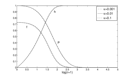
(a) matter functions $P(r)$, $h(r)$, $f(r)$

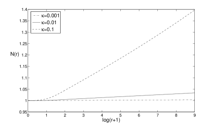
(b) metric function $N(r)$

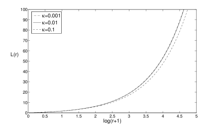
(c) metric function $L(r)$

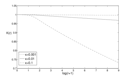
(d) metric function $K(r)$

Figure 1: The matter and metric functions for a gravitating superconducting string with ${\rm w}=-0.3$, $\gamma_{2}=3$, $\gamma_{3}=2$, $q=0.7$, $\alpha=0.1$ and different values of $\kappa$.

The outside space-time of a superconducting string should be given by the Kasner space-time with a specific relation between the Kasner coefficients and $U$ and $T$ (see (31)) patrick1 . We observe that our numerical solutions indeed possess an asymptotic behaviour governed by the Kasner metric (28). Matching the space-time of the solution given in Fig.1 at large $r$ with the Kasner metric we find $a=0.00040092$, $b=-0.00040076$, $c=-0.00000054$ for $\kappa=0.001$ and $a=0.04098961$, $b=-0.03937305$, $c=-0.00165716$ for $\kappa=0.1$, respectively.

In Fig.2 we give the values of the Kasner coefficients in dependence on $\kappa(U-T)$ for a superconducting string with timelike current (the results are qualitatively similar in the spacelike case, this is why we do not present them here) and $\gamma_{2}=3$, $\gamma_{3}=1.74$, $q=0.69$, $\alpha=0.1$. For small values of $\kappa$ we recover the behaviour given in (31). For larger values of $\kappa$ the parameter $c$ starts to deviate from zero, while $a$ and $b$ no longer depend linearly on $\kappa(U-T)$. We hence conclude that for small values of $\kappa(U-T)$ the description of the metric outside the superconducting string by a Kasner metric with the identification (31) is a very good approximation. However, with our techniques, we are also able to determine the behaviour of the metric functions inside the string core up to the string axis at $r=0$. This is only possible when solving the equations of motion numerically. In the following, we want to discuss the macroscopic stability of gravitating superconducting strings. For this, we will need to integrate the matter and metric functions from $r=0$ to $r=\infty$. It is hence crucial to know the matter and metric functions on the full interval $r\in[0:\infty[$.

Figure 2: We show the value of the Kasner coefficients $a$, $b$ and $c$ for gravitating superconducting string solutions with timelike current and $\gamma_{2}=3$, $\gamma_{3}=1.74$, $q=0.69$, $\alpha=0.1$ in dependence on $\kappa(U-T)$. We give the coefficients for two different values of ${\rm w}$.

III.2 Macroscopic stability

In flat space-time it was found patrick3 that in the spacelike regime ${\rm w}>0$ the energy per unit length $U$ and the tension $T$ are always positive and hence $c_{\rm T}^{2}>0$. However, while the energy per unit length is an increasing function of ${\rm w}$ in the spacelike regime, the tension $T$ decreases only for ${\rm w}$ close to the chiral limit ${\rm w}=0$. For sufficiently small ${\rm w}$ it was hence found that the strings are stable with $c_{\rm L}^{2}>0$, while for larger values $c_{\rm L}^{2}<0$. In the timelike regime, the energy per unit length and tension diverge at the approach of the phase frequency threshold which corresponds to the value of $-{\rm w}$ equal to the mass of the scalar boson. In the following, we have fixed $\gamma_{2}=3$, $\gamma_{3}=2$, $\alpha=0.1$, $q=0.7$ unless otherwise stated. This choice of parameters fulfills all the requirements such that the local $U(1)$ symmetry is broken and the global $U(1)$ symmetry remains unbroken in the flat space-time limit. In the following, we will be interested in the way that the energy per unit length $U$, the tension $T$ as well as the charge number density $J$ change with $\kappa$. In Fig.3 we plot $U$ and $T$ as function of ${\rm w}$ for ${\rm w}$ close to ${\rm w}=0$. For $\kappa=0$ we recover the results given in patrick3 .

Figure 3: We show the energy per unit length $U$ (black) as well as the tension $T$ (red) as function of ${\rm w}=k^{2}-\omega^{2}$ for superconducting strings for different values of $\kappa$ and $\gamma_{2}=3$, $\gamma_{3}=2$, $q=0.7$ and $\alpha=0.1$.

Note that we plot the dependence on ${\rm w}$ and not on ${\rm sgn(w)}\sqrt{\rm|w|}$. We do not present our results in dependence on this latter quantity here, but have convinced ourselves that the plots look qualitatively similar to those presented in patrick3 . We observe that the main features are still present for $\kappa\neq 0$. The value of ${\rm w}={\rm w}_{\rm cr}^{0}$ at which $T=U$ in the spacelike regime corresponds to the value of ${\rm w}$ where $f(0)=0$ and hence $f(r)\equiv 0$. We find that ${\rm w}_{\rm cr}^{0}$ increases with $\kappa$, as do the corresponding values of $U$ and $T$. This leads also to the observation that the range of ${\rm w}$ in the spacelike regime for which $c_{\rm L}^{2}>0$ increases since the minimal value of $T$ appears at larger values of ${\rm w}$. Hence, the coupling to gravity enhances the interval of ${\rm w}\geq 0$ in which strings are stable. This is also seen in Fig.4, where we plot $T$ as function of $U$. Obviously, $dT/dU<0$ for ${\rm w}$ close to the chiral limit ${\rm w}=0$. We also give the charge number density $J$ in Fig.5. This shows that this quantity vanishes at ${\rm w}_{\rm cr}^{0}$ as well as at ${\rm w}=0$. In the spacelike regime the charge number density first rises reaching a maximum at ${\rm w}_{\rm max}$ and then decreases again to zero at ${\rm w}_{\rm cr}^{0}$. We find that ${\rm w}_{\rm max}$ increases with $\kappa$. In the timelike regime the charge number density rises strongly and the bigger $\kappa$ the bigger $J$ for a given value of ${\rm w}$.

Figure 4: We show the tension $T$ as function of the energy per unit length $U$ for superconducting strings for different values of $\kappa$ and $\gamma_{2}=3$, $\gamma_{3}=2$, $q=0.7$ and $\alpha=0.1$.

Figure 5: We show the charge number density $J$ as function of ${\rm w}=k^{2}-\omega^{2}$ for superconducting strings for different values of $\kappa$ and $\gamma_{2}=3$, $\gamma_{3}=2$, $q=0.7$ and $\alpha=0.1$.

Figure 6: We show $U$ as function of $-{\rm w}$ for different values of $\kappa$ and $\gamma_{2}=3$, $\gamma_{3}=2$, $q=0.7$ and $\alpha=0.1$.

Figure 7: We show $U$ and $T$ as function of $-{\rm w}$ for $\kappa=0.3$ and $\gamma_{2}=3$, $\gamma_{3}=2$, $q=0.7$ and $\alpha=0.1$. The small subfigures show the energy per unit length $U$ and the tension $T$, respectively at large $-{\rm w}$. Clearly, $U$ decreases, while $T$ increases and becomes positive for sufficiently large $-{\rm w}$ signaling the stability of the superconducting string.

In the timelike regime we find in analogy with patrick3 that there exists a phase frequency threshold at which $U\rightarrow+\infty$ and $T\rightarrow-\infty$ for $\kappa=0$. This corresponds to the value of ${\rm w}$ at which scalar bosons can be produced. Interestingly, we observe that this phase frequency threshold seems to be absent when $\kappa\neq 0$. This is shown in Fig.6, where we give $U$ as function of ${\rm w}$ in the timelike regime. Clearly, for large values of $-{\rm w}$ the energy per unit length tends to a finite value for $\kappa\neq 0$. Interestingly, we find that the coupling to gravity can hence stabilize the strings. This is shown in Fig.7, where we present $U$ and $T$ in the timelike regime for $\kappa=0.3$. In an interval close to ${\rm w}=0$ we find that both $U$ and $T$ are positive with $U$ increasing and $T$ decreasing such that $c_{\rm L}^{2}>0$ and $c_{\rm T}^{2}>0$. Hence, the strings are stable. Decreasing ${\rm w}$ further leads to $T$ becoming negative such that while $c_{\rm L}^{2}>0$ we now have $c_{\rm T}^{2}<0$ and the strings are unstable. However, in contrast to the flat space-time case, where $c_{\rm T}^{2}<0$ up to the phase frequency threshold, we observe that for sufficiently small ${\rm w}$ the tension becomes positive again. As such $c_{\rm T}^{2}>0$. Furthermore, for these values of ${\rm w}$ we find that $U$ decreases, while $T$ increases such that $c_{\rm L}^{2}>0$ and the strings are macroscopically stable. We conclude that there are hence two stable regions in the timelike regime for $\kappa\neq 0$. Hence, gravity can stabilize the strings for large values of the current. To get an idea how the parameter ranges in which the string becomes stable depend on $\kappa$, we show the values of ${\rm w}$ where $T=0$ in dependence on $\kappa$ in Fig.8. In between the two curves the tension $T$ is negative and hence $c_{\rm L}^{2}$ is negative. We observe that the value of ${\rm w}$ close to ${\rm w}=0$ at which $T$ vanishes and $dT/d{\rm w}<0$ increases with increasing $\kappa$. On the other hand, the value of ${\rm w}$ at which $T$ vanishes and $dT/d{\rm w}>0$ decreases with increasing $\kappa$. Hence, the range ${\rm w}$ for which $c_{\rm T}^{2}<0$ decreases with increasing $\kappa$. Furthermore, our numerical results indicate that $c_{\rm T}^{2}>0$ for all ${\rm w}$ if $\kappa$ is sufficiently large. For $\gamma_{2}=3$, $\gamma_{3}=2$, $\alpha=0.1$, $q=0.7$ we find that this happens at $\kappa\approx 0.16$.

Figure 8: We show the region in the ${\rm w}$-$\kappa$ domain for which $T<0$ (and hence $c_{T}^{2}<0$). Note that for $\kappa=0$ the tension $T>0$ in the spacelike regime. This changes when considering the superconducting string in curved space-time for sufficiently small, but non-vanishing $\kappa$. This is for $\gamma_{2}=3$, $\gamma_{3}=2$, $q=0.7$ and $\alpha=0.1$.

IV Motion of test particles

In order to probe space-times it is crucial to understand how test particles move in these. We here consider structure-less, point-like particles that move on geodesics in the gravitational field of a superconducting string. If we consider the numerically given space-time in terms of the metric functions $N$, $L$ and $K$ we have to solve the geodesic equation numerically. This approach has been taken in hartmann_sirimachan for standard cosmic strings and it was found that the finite core width of the string allows for additional bound orbits of massive test particles close to the string core. Since the string core and hence also the radius of the orbits are on the same order as the inverse scalar boson mass these cannot account for planetary orbits. On the other hand, the string could be “dressed” by massive particles and this could be important for gravitational wave emission. However, our numerical results indicate that the power of this emission would be rather small. This is why we do not investigate this further here.

As shown above, we find that the metric outside the string core is well matched by the Kasner space-time. Since this space-time can be given analytically we are able to make some general statements about the geodesic motion.

Since the observation of gravitational lensing by a cosmic string has been suggested as a possibility to detect these objects directly, we discuss the motion of massless test particles in the Kasner space-time in the following. We also comment on the motion of massive test particles.

IV.1 The geodesic equation

The Kasner metric has three obvious Killing vectors: $\partial_{t}$, $\partial_{\theta}$ and $\partial_{z}$. The three associated constants of motion are:

$$P_{t}=-\left(\frac{r}{r_{\sigma}}\right)^{2a}\frac{dt}{d\lambda}\ \ ,\ \ P_{z}=\left(\frac{r}{r_{\sigma}}\right)^{2b}\frac{dz}{d\lambda}\ \ ,\ \ P_{\theta}=\gamma r^{2}\left(\frac{r}{r_{\sigma}}\right)^{2c}\frac{d\theta}{d\lambda}\ ,$$ (32)

where $\lambda$ is an affine parameter that can be identified with proper time for time-like geodesics. $P_{t}$ corresponds to the energy, $P_{z}$ to the linear momentum in the $z$-direction and $P_{\theta}$ to the angular momentum of a test particle moving in this space-time, respectively. The geodesic Lagrangian then reads

$${\cal L}_{\rm geo}=\frac{1}{2}g_{\mu\nu}\frac{dx^{\mu}}{d\lambda}\frac{dx^{\nu}}{d\lambda}=\frac{1}{2}\epsilon\ ,$$ (33)

where $\epsilon$ takes the value $0$ and $1$ for massless and massive particles, respectively. Using the constants of motion (32) the equation of motion for $r$ reads

$$P_{t}\frac{dt}{d\lambda}+P_{z}\frac{dz}{d\lambda}+P_{\theta}\frac{d\theta}{d\lambda}+\left(\frac{dr}{d\lambda}\right)^{2}=-\epsilon$$ (34)

which can be rewritten as follows

$$\left(\frac{dr}{dt}\right)^{2}+\left[-\left(\frac{r}{r_{\sigma}}\right)^{2a}+\frac{\epsilon}{P_{t}^{2}}\left(\frac{r}{r_{\sigma}}\right)^{4a}+\left(\frac{P_{z}}{P_{t}}\right)^{2}\left(\frac{r}{r_{\sigma}}\right)^{4a-2b}+\frac{1}{\gamma r^{2}}\left(\frac{r}{r_{\sigma}}\right)^{4a-2c}\left(\frac{P_{\theta}}{P_{t}}\right)^{2}\right]=0\ .$$ (35)

The dynamics is thus similar to that of a classical point particle of unit mass and zero total energy subject to the effective potential:

$$V_{\rm eff}(r) = \frac{1}{2}\left[-\left(\frac{r}{r_{\sigma}}\right)^{2a}+\frac{\epsilon}{P_{t}^{2}}\left(\frac{r}{r_{\sigma}}\right)^{4a}\right.\left.+\left(\frac{P_{z}}{P_{t}}\right)^{2}\left(\frac{r}{r_{\sigma}}\right)^{4a-2b}+\frac{1}{\gamma r^{2}}\left(\frac{P_{\theta}}{P_{t}}\right)^{2}\left(\frac{r}{r_{\sigma}}\right)^{4a-2c}\right]$$ (36)

The equations for $\theta$ and $z$ are directly obtained from the constants of motion and read

$$\frac{dz}{dt}=-\frac{P_{z}}{P_{t}}\left(\frac{r}{r_{\sigma}}\right)^{2(a-b)}\ \ ,\ \ \frac{d\theta}{dt}=-\frac{1}{\gamma r^{2}}\frac{P_{\theta}}{P_{t}}\left(\frac{r}{r_{\sigma}}\right)^{2(a-c)}\ .$$ (37)

IV.2 The effective potential

Some properties of the orbits can be deduced from the form of the effective potential. First note that $V_{\rm eff}<0$ in order for (35) to have solutions.

In the following we will discuss the possible orbits in this space-time. We will define bound, i.e. planetary orbits as orbits on which particles move from a maximal finite radius $r_{\rm max}$ to a minimal radius $r_{\rm min}>0$ and back again in the $x$-$y$-plane. Note that these orbits can extend to infinity in the $z$-direction for $P_{z}\neq 0$. In contrast to that we have unbound orbits on which particles approach the string from infinity, move to a minimal radius $r_{\rm min}$ and then return to infinity in the $x$-$y$-plane. In both cases, it is also of interest to know whether $r_{\rm min}$ can become zero, i.e. whether the particle can reach the string axis. In the following, we will call orbits that end at $r_{\rm min}=0$ “terminating orbits”. The possible orbits are summarized in Table I.

type	turning points	range of r	orbit
A	0	(-2,-0.2)(3,0.2)[linewidth=0.5pt]-¿(-2,0)(3,0) [linewidth=1.2pt](-2,0)(3,0)	terminating escape orbit
B	1	(-2,-0.2)(3,0.2)[linewidth=0.5pt]-¿(-2,0)(3,0) [linewidth=1.2pt]-*(-2,0)(0,0)	terminating orbit
C	2	(-2,-0.2)(3,0.2)[linewidth=0.5pt]-¿(-2,0)(3,0) [linewidth=1.2pt]*-*(-0.5,0)(1.5,0)	bound orbit
D	1	(-2,-0.2)(3,0.2)[linewidth=0.5pt]-¿(-2,0)(3,0) [linewidth=1.2pt]*-(0.5,0)(3,0)	escape orbit

Table 1: Types of possible orbits for test particles moving in the static Kasner space-time.

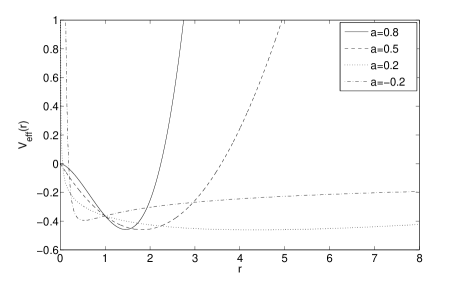
(a) effective potential $V_{\rm eff}(r)$ for $b^{+}$, $c^{+}$

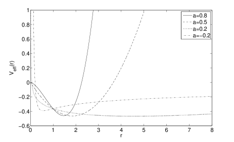
(b) effective potential $V_{\rm eff}(r)$ for $b^{-}$, $c^{-}$

Figure 9: We show the effective potential $V_{\rm eff}(r)$ for a massive test particle ($\epsilon=1$) with $P_{t}=2$, $P_{z}=P_{\theta}=0.2$ in a Kasner space-time with $r_{\sigma}=1$, $\gamma=0.8$ and different choices of $a$. Note that the Kasner conditions then fix the possible values of $b$ and $c$. We show the effective potential for $b^{+}$, $c^{+}$ (left) as well as for $b^{-}$, $c^{-}$ (right).

$a$

$<0$

$0$

$>0$ and $<2/3$

$>2/3$

$\epsilon$

$0$

$-1$

$0$

$-1$

$0$

1

$P_{z}$

$0$

$\neq 0$

$0$

$\neq 0$

$0$

$\neq 0$

$0$

$\neq 0$

$0$

$\neq 0$

$P_{\theta}$

$0$

$\neq 0$

$0$

$\neq 0$

$0$

$\neq 0$

$0$

$\neq 0$

type

A

D

D

D

A

D

A

B

D

C

B

C

A

B

B

B

Table 2: Types of orbits in the static Kasner space-time in dependence on the different parameters for the $(b^{+},c^{+})$ solution. The table for $(b^{-},c^{-})$ would be the same with $P_{z}$ and $P_{\theta}$ exchanged.

In Fig.9 and Fig.10 we show the effective potential $V_{\rm eff}(r)$ for massive and massless particles, respectively, with $P_{t}=2$, $P_{z}=P_{\theta}=0.2$ in the space-time of a Kasner metric with $r_{\sigma}=1$, $\gamma=0.8$ and different choices of $a$. The choice of $a$ fixes the value of $b$ and $c$ (see (30)). We give the potential for both choices of $b$ and $c$ and note that the difference between the two choices is marginal. For general choices of $a$ our results are summarized in Table II. These are:

• If $a<0$, there are no bound orbits since the potential has no local maximum and is negative at infinity. This is clearly seen in Fig.9 and Fig.10 for $a=-0.2$. In addition, the minimal radius $r_{\rm min}$ is finite, except for a massless particle with vanishing $P_{z}$ and $P_{\theta}$. In this case, $V_{\rm eff}(r)\propto r^{2a}$ for $r\rightarrow 0$. Since $a<0$, $\frac{dt}{dr}\propto\frac{1}{\sqrt{V_{\rm eff}}}\propto r^{-a}$ is integrable around $r=0$ and the particle thus reaches the string after a finite coordinate time.

• For $a=0$, there are no bound orbits. This corresponds either to the case of a standard cosmic string in which case the space-time is locally flat with $b=b^{-}=c^{-}=c=0$ or to $b=b^{+}=-c^{+}=-c=1$ which is not physical. The minimal radius $r_{\rm min}$ is generally finite, except if $P_{z}=0$ (for $b^{+}$, $c^{+}$) or $P_{\theta}=0$ (for $b^{-}$, $c^{-}$), in which case the potential is just a constant.

• For $a>0$ and $\epsilon=1$ (massive particle): the orbits are always bound if $a<2/3$ and $P_{z}\neq 0$ (for $b^{+}$, $c^{+}$) or $a<2/3$ and $P_{\theta}\neq 0$ (for $b^{-}$, $c^{-}$). This is clearly seen in Fig.9 for $a=0.2$ and $a=0.5$, where the potential in both cases has positive values close to $r=0$ and tends to positive values at $r\rightarrow\infty$. For other choices of $a$ the orbits are bound terminating, i.e. end at the string axis at $r=0$ since the potential tends to zero from below at $r\rightarrow 0$ (see the potential for $a=0.8$ in Fig.9). When the minimal radius vanishes, the dominant term near $r=0$ is at least $r^{2a}$. So, $\frac{dt}{dr}=\mathcal{O}(r^{-a})$. Since $a<1$, this is integrable around $r=0$ and the time needed to reach the string is finite (except if $a=1$).

• For $a>0$ and $\epsilon=0$ (massless particle): the behaviour around $r=0$ is exactly the same as in the massive case (since the removed term is negligible), but the orbits are unbound for $a\leq 2/3$ when choosing $P_{\theta}=0$ for ($b^{+}$, $c^{+}$) or $P_{z}=0$ for ($b^{-}$, $c^{-}$). This is seen in Fig.10. This means that for appropriate choices of the parameters, we find that bound orbits for massless test particles exist.

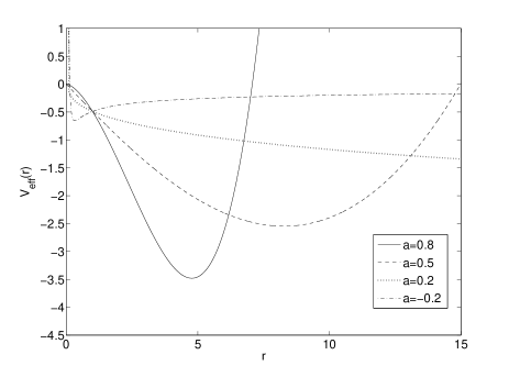
(a) effective potential $V_{\rm eff}(r)$ for $b^{+}$, $c^{+}$

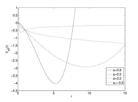
(b) effective potential $V_{\rm eff}(r)$ for $b^{-}$, $c^{-}$

Figure 10: We show the effective potential $V_{\rm eff}(r)$ for a massless test particle ($\epsilon=0$) with $P_{t}=2$, $P_{z}=P_{\theta}=0.2$ in a Kasner space-time with $r_{\sigma}=1$, $\gamma=0.8$ and different choices of $a$. Note that the Kasner conditions then fix the possible values of $b$ and $c$. We show the effective potential for $(b^{+}$, $c^{+})$ (left) as well as for $(b^{-}$, $c^{-})$ (right).

We remark that exchanging $P_{\theta}$ and $P_{z}$ does not change the qualitative form of the potential, provided we also exchange $(b^{+},c^{+})$ with $(b^{-},c^{-})$. In fact, the equation of motion for $r$ is invariant under

$$(b^{+},c^{+})\leftrightarrow(b^{-},c^{-})\ \ ,\ \ P_{z}\leftrightarrow\frac{P_{\theta}}{\sqrt{\gamma r_{\sigma}^{2}}}$$ (38)

so that we can restrict our attention to one of the two cases.

Studying the asymptotic properties of $V_{\rm eff}$ is a priori not enough to rule out bound orbits, or to say that there is only one bound orbit (the potential could cross zero several times in the intermediate region.) However, we find that nothing new arises from a more detailed study.

Note that the case of interest in the context of cosmic strings with additional structure corresponds to $a>0,a\approx 0,b=b^{-}\approx-a,c=c^{-}\approx 0$.

IV.3 Numerical results

The equations of motion are solved numerically using a second-order symplectic integrator, which avoids numerical dissipation effects. We studied the domain of existence and the dependence of the maximal and minimal radius on the Kasner coefficients and constants of motion, as well as the light deflection using Maple and Mathematica.

IV.3.1 Domain of existence

Given the parameters $a$, $b$ and $c$ in the Kasner metric, a natural question is what values of $\gamma$, $P_{t}$, $P_{z}$ and $P_{\theta}$ allow for solutions of the equations of motion. A necessary and sufficient condition is that the potential must be negative somewhere. For $a<0$ or $a>2/3$, the dominant term at zero or infinity respectively is $-\frac{1}{2}\left(\frac{r}{r_{\sigma}}\right)^{2a}$. Therefore, solutions always exist. For $a\in\left]0,2/3\right[$, the domain in which solutions exist can be computed numerically. For massless particles, since $r_{\sigma}$ can be taken equal to one by rescaling $r$ and $\gamma$ can be taken to one by rescaling $P_{\theta}$, the function $r\mapsto V_{\rm eff}(r)$ depends only on two parameters, for instance on $P_{z}/P_{t}$ and $P_{\theta}/P_{t}$ for $r_{\sigma}=1$, $\gamma=1$. Moreover, because of the aforementioned duality, we can restrict our attention to the $(b^{-},c^{-})$ solution. For massive particles, $P_{t}$ becomes a physically relevant parameter. The domain in which solutions exist tend towards the one obtained for $\epsilon=0$ in the limit $P_{t}\rightarrow\infty$ and shrink when $P_{t}$ decreases. For $a=0$, we found analytically that solutions exist if and only if $P_{z}^{2}+\epsilon\leq P_{t}^{2}$ for the $(b^{+},c^{+})$ case or $\frac{P_{\theta}^{2}}{\gamma}+\epsilon\leq P_{t}^{2}$ for the $(b^{-},c^{-})$ case (in units $r_{\sigma}=1$). For $a=2/3$, these conditions become $\left(\frac{P_{z}}{P_{t}}\right)^{2}\leq 1$ or $\frac{1}{\gamma}\left(\frac{P_{\theta}}{P_{t}}\right)^{2}\leq 1$ for the $(b^{+},c^{+})$ and $(b^{-},c^{-})$ case respectively. Our results are summarized in Fig.11 for massless particles and particular choices of $P_{t}$.

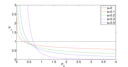
(a) $P_{t}=1$

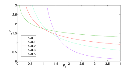
(b) $P_{t}=2$

Figure 11: We show the domain of existence of solutions to the geodesic equation in the $P_{\theta}$-$P_{z}$-plane in a general Kasner space-time with $r_{\sigma}=1$, $\gamma=1$ and different values of $a$ for massless test particles with $P_{t}=1$ (left) and $P_{t}=2$ (right). Note that solutions to the geodesic equation exist below and to the left of the curves.

IV.3.2 Examples of orbits

The most important difference to the case $T=U$ in which geodesics are just straight lines because the space-time is locally flat is that we can have bound orbits for massive and massless test particles in the general Kasner space-time. In Fig.12 we show bound orbits for a massive and massless test particle, respectively. The bound orbit of a massive test particle shows the typical perihelion shift of orbits in curved space-time. The bound orbit of the massless test particle also possesses this perihelion shift, however looks qualitatively rather like a spiral. We observe that this in related to the choice of $a$, which is quite big. For $a$ small the orbit of a massless particle looks qualitatively similar to that of a massive one.

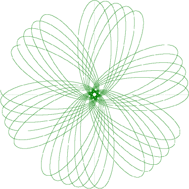
(a) massive test particle, $P_{t}=2$, $P_{z}=0$, $P_{\theta}=0.5$ , $a=0.3$, $b=-0.2266281297$, $c=-0.07337187027$ and $\gamma=0.5$

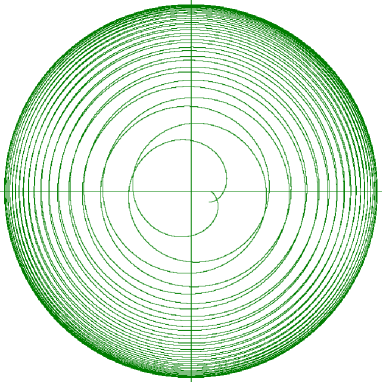
(b) massless test particle, $P_{t}=2.0$, $P_{z}=0.1$, $P_{\theta}=0.03$ , $a=0.8$, $b=0.512311$, $c=-1.31231$ and $\gamma=0.8$

Figure 12: We show a bound orbit for a massive (left) and a massless (right) test particle in a Kasner space-time.

In Fig.13 we show escape orbits for a massive and massless test particle, respectively. In both cases, the test particles get deflected by the string, which is related to the presence of the deficit angle of the space-time. We observe that the massive test particle experiences a stronger deflection for the same values of all parameters as the massless one.

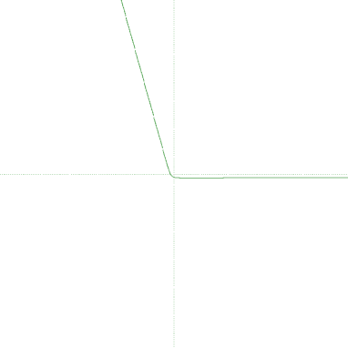
(a) massive test particle

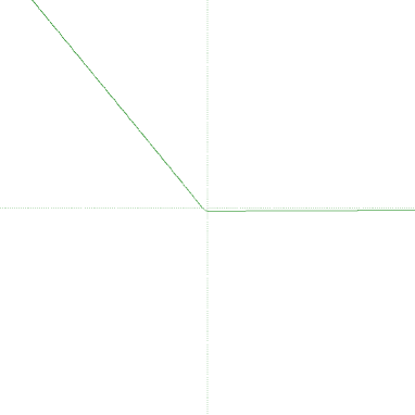
(b) massless test particle

Figure 13: We show escape orbits for a massive test particle (left) and a massless test particle (right) for $P_{t}=2$, $P_{z}=0.1$, $P_{\theta}=0.2$ , $a=0$, $b=b_{-}$ and $c=c_{-}$ and $\gamma=0.5$ in a Kasner space-time.

IV.3.3 Minimal and maximal radius of bound orbits

If the momenta are held fixed, the minimal and maximal radii of the bound orbits are decreasing functions of $a$. The maximal radius generally goes to infinity when $a\rightarrow 0^{+}$, while the minimum radius remains finite. This was to be expected since the orbits are unbound with finite minimal radius for $a<0$ (let alone the very special case $P_{\theta}=P_{z}=0$). For $a>2/3$ and fixed $P_{\theta}$, $P_{t}$, we find terminating bound orbits. The maximal radius decreases with $P_{z}$, going to zero at infinity. It remains finite as $P_{z}\rightarrow 0$, which was also expected from the above analysis. For $0<a<2/3$, there are two critical values of $P_{z}$ above which the equations of motion can not be satisfied for $(b^{+}$, $c^{+})$ or $(b^{-}$, $c^{-})$. The minimal and maximal radius merge at this point, and move apart from each other when we decrease $P_{z}$. The merging of the minimal and maximal radius corresponds to a local minimum of the effective potential. If we consider the $(b^{+},c^{+})$ case, the maximal radius remains finite when $P_{z}\rightarrow 0$, while the minimum one goes to zero. For the $(b^{-},c^{-})$ case, it is $r_{min}$ which remains finite while $r_{max}$ goes to infinity if $\epsilon=0$. For $a<0$, we find no maximal radius, and the minimal one increases with $P_{z}$. In Fig.14 we show the minimal and maximal radius of the bound orbits for a Kasner space-time with $a=0.3$, $b=-0.2266281297$, $c=-0.073371870270$ and $\gamma=0.5$ in dependence on $P_{\theta}$. The test particle has $P_{t}=2$ and three different values of $P_{z}$. The $r_{\rm min}$ and $r_{\rm max}$ curves meet at the circular orbit. We find that the interval of $P_{\theta}$ for which bound orbits exist increases when decreasing $P_{z}$ for a fixed $P_{t}$. Moreover, we observe that the radius of the circular orbit decreases with increasing $P_{z}$. In addition, the circular orbit appears at smaller angular momentum $P_{\theta}$ when increasing $P_{z}$.

Figure 14: The value of the minimal radius $r_{\rm min}$ and of the maximal radius $r_{\rm max}$ of bound orbits of massive test particles $(\epsilon=1$) with $P_{t}=2$ in a Kasner space-time with $a=0.3$, $b^{-}$, $c^{-}$, $\gamma=0.5$ are shown in dependence of $P_{\theta}$ for three different values of $P_{z}$.

IV.3.4 Light deflection

For an unbound orbit, we can define the deviation angle as:

$$\Delta\theta=2\int_{r_{min}}^{\infty}\left|\frac{d\theta}{dr}\right|\,dr-\pi=\frac{\sqrt{2}}{\gamma}\frac{P_{\theta}}{P_{t}}\int_{r_{min}}^{\infty}\frac{1}{r^{2}}\left(\frac{r}{r_{\sigma}}\right)^{2a-2c}\frac{1}{\sqrt{-V_{\rm eff}}}dr-\pi$$ (39)

where $r_{min}$ is the minimal distance from the string to the particle.

If all the other parameters are fixed, $\Delta\theta$ is a decreasing function of $\gamma$. It goes to infinity when $\gamma\rightarrow 0$ and is equal to $\left(\frac{1}{\sqrt{\gamma}}-1\right)\pi$ in conical space-time. (This is true in a coordinate system in which the metric has the Kasner form and $\theta$ goes from $0$ to $2\pi$. A geometrical argument shows that it reduces to the usual $2\pi(1-\sqrt{\gamma})$ in a locally flat coordinate system.)

For $a>0$, the $(b^{-},c^{-})$ case gives an unbound orbit for massless particles with vanishing $P_{z}$. We find that the deviation angle increases with $a$.

The deviation angle also seems to behave logarithmically in $P_{\theta}$ in the limit $P_{\theta}\rightarrow\infty$. For $P_{\theta}\rightarrow 0$ we have $\Delta\theta\rightarrow-\pi$. This is related to the repulsive effect of the string: if the angular momentum vanishes, the particle just goes back to where it comes from.

V Summary and discussions

In this paper we have studied superconducting string solutions of the $U(1)_{\rm local}\times U(1)_{\rm global}$ model in curved space-time. For small values of the ratio between the symmetry breaking scale and the Planck mass we find that the metric outside the string core matches the Kasner metric very well and the Kasner coefficients can be given in terms of the energy per unit length $U$ and the tension $T$ as originally suggested in patrick1 . In order to be able to decide about the macroscopic stability of these objects using the stability conditions given by Carter carter ; carter2 we have to know the metric functions on the full interval $r\in[0:\infty[$. We have hence integrated the full coupled system of differential equations numerically and computed the energy per unit length and tension. We find that the coupling to gravity can stabilize the strings with large charge number density for sufficiently large values of the ratio between the symmetry breaking scale and the Planck mass and that in general the phase frequency threshold is absent in curved space-time. As such, the energy per unit length and tension never diverge, but tend to more or less constant values for larger values of the charge number density.

We have also studied the motion of test particles in the general Kasner space-time and find that the fact that the energy per unit length is non-equal to the tension can lead to bound orbits of massive and massless test particle. The question is then whether these orbits are of interest for astrophysical or cosmological applications. We find that the radius of these orbits is too large to be of interest and that e.g. the gravitational wave emission from a particle moving on a bound orbit around a cosmic string would be far too small to be detectable. This – in turn – means that the assumption of an infinitely thin cosmic string that is often used in simulations of string networks is a valid assumption and that the additional structure on the string does not have a big influence on the results.

Acknowledgments We would like to thank Patrick Peter for many fruitful and enlightening discussions as well as the Institut d’Astrophysique de Paris (IAP) where part of this work was carried out for its hospitality. This work was partially funded by Deutsche Forschungsgemeinschaft (DFG) grant HA-4426/5-1. BH also gratefully acknowledges support within the framework of the DFG Research Training Group 1620 Models of gravity. FM would like to thank the École Normale Supérieure, Paris, France.

References

- (1) T. Kibble, J. Phys. A 9, 1378 (1976).
- (2) see e.g. M. B. Hindmarsh and T. W. B. Kibble, Rept. Prog. Phys. 58, 477 (1995).
- (3) P. Peter and J.-P. Uzan, Primordial Cosmology, Oxford University Press, 2009.
- (4) see e.g. J. Polchinski, Introduction to cosmic F- and D-strings, hep-th/0412244 and reference therein.
- (5) M. Majumdar and A. C. Davis, JHEP 0203, 056 (2002); S. Sarangi and S. H. H. Tye, Phys. Lett. B 536, 185 (2002).
- (6) D.H. Lyth and A. Riotto, Phys. Rept. 314, 1 (1999).
- (7) R. Jeannerot, J. Rocher and M. Sakellariadou, Phys. Rev. D 68, 103514 (2003).
- (8) P.M. Saffin, JHEP 0509, 011 (2005).
- (9) A. Rajantie, M. Sakellariadou and H. Stoica, JCAP 11, 021 (2007).
- (10) P. Salmi et al, Phys. Rev. D 77, 041701 (2008).
- (11) J. Urrestilla and A. Vilenkin, JHEP 0802, 037 (2008).
- (12) H. B. Nielsen and P. Olesen, Nucl. Phys. B 61, 45 (1973).
- (13) E. Witten, Nucl. Phys. B 249, 557 (1985).
- (14) P. Peter, Phys. Rev. D 45, 1091 (1992).
- (15) B. Carter, Phys. Lett.B 228 466 (1989).
- (16) B. Carter, in Formation and Evolution of Cosmic strings, edited by G. W. Gibbons, S. W. Hawking and T. Vachaspati, Cambridge University Press, 1990.
- (17) B. Hartmann and B. Carter, Phys. Rev. D 77, 103516 (2008).
- (18) F. R. Bouchet, P. Peter, A. Riazuelo and M. Sakellariadou, Phys. Rev. D 65, 021301 (2002).
- (19) N. Bevis et al, Phys. Rev. D75, 065015 (2007); N. Bevis et al, arXiv:astro-ph/0702223; N. Bevis et al, Phys. Rev. D76, 043005 (2007); N. Bevis, M. Hindmarsh, M. Kunz and J. Urrestilla, Phys. Rev. Lett. 100, 021301 (2008); Phys. Rev. D 75, 065015 (2007); Phys. Rev. D 82, 065004 (2010); JCAP 1112, 021 (2011)
- (20) J. Urrestilla, P. Mukherjee, A. R. Liddle, N. Bevis, M. Hindmarsh and M. Kunz, Phys. Rev. D 77, 123005 (2008); Phys. Rev. D 83, 043003 (2011).
- (21) B. Hartmann and P. Sirimachan, JHEP 1008, 110 (2010).
- (22) P. Peter and D. Puy, Phys. Rev. D 48 (1993) 5546.
- (23) J. Garriga and P. Peter, Class. Quant. Grav. 11, 1743 (1994).
- (24) P. Peter, Class. Quant. Grav. 11, 131 (1994).
- (25) see e.g. D. Kramer, H. Stephani, E. Herlt and M. MacCallum, Exact solutions of Einstein’s field equations, Cambridge University Press, 1980.
- (26) N. Ozdemir, Gen. Rel. Grav. 33, 603 (2001).
- (27) M. Christensen, A. L. Larsen and Y. Verbin, Phys. Rev. D 60, 125012 (1999).
- (28) Y. Brihaye and M. Lubo, Phys. Rev. D 62, 085004 (2000).
- (29) U. Ascher, J. Christiansen and R. D. Russell, Math. Comput. 33 (1979), 659; ACM Trans. Math. Softw. 7, 209 (1981).