Scalar field quantum cosmology: a Schrödinger picture

Abstract

We study the classical and quantum models of a scalar field Friedmann-Robertson-Walker (FRW) cosmology with an eye to the issue of time problem in quantum cosmology. We introduce a canonical transformation on the scalar field sector of the action such that the momentum conjugate to the new canonical variable appears linearly in the transformed Hamiltonian. Using this canonical transformation, we show that, it may lead to the identification of a time parameter for the corresponding dynamical system. In the cases of flat, closed and open FRW universes the classical cosmological solutions are obtained in terms of the introduced time parameter. Moreover, this formalism gives rise to a Schrödinger-Wheeler-DeWitt equation for the quantum-mechanical description of the model under consideration, the eigenfunctions of which can be used to construct the wave function of the universe. We use the resulting wave functions in order to investigate the possible corrections to the classical cosmologies due to quantum effects by means of the many-worlds and ontological interpretation of quantum cosmology.
PACS numbers: 98.80.Qc, 04.60.Ds
Keywords: Scalar field cosmology, Quantum cosmology, Problem of time

1 Introduction

Since $1967$ when canonical quantum theory of gravity was first introduced by DeWitt [1], many efforts have been made in this area and the corresponding results have been followed by a number of works, the main motivations of which lie in the results of the unification theories and cosmology [2]. The main object of such a theory, i.e., the quantum state of the gravitational system, is then described by a wave function, a functional (on superspace) of the $3$-geometry and matter fields presented in the theory, satisfying the Wheeler-DeWitt (WDW) equation [3]. One of the most important features related to the WDW wave function is a problem which is known as the ”problem of time”. Indeed, unlike the case of usual quantum theory, the wave function in quantum gravity is independent of time, which is a reflect to the fact that general relativity is a parameterized theory in the sense that its (Einstein-Hilbert) action is invariant under time reparameterization. Because the existence of this problem, the canonical formulation of general relativity leads to a constrained system, and its Hamiltonian is a superposition of some constraints, the so-called Hamiltonian and momentum constraints. A possible way to overcome this problem is that one first solves the equation of constraint to obtain a set of genuine canonical variables with which one can construct a reduced Hamiltonian. In this kind of time reparameterization, the equations of motion are obtained from the reduced physical Hamiltonian and describe the evolution of the system with respect to the selected time parameter [4].

The problem of time was first addressed in [1] by DeWitt himself. However, he argued that the problem of time should not be considered as a hindrance in the sense that the theory itself must include a suitable well-defined time in terms of its geometry or matter fields. In this scheme time is identified with one of the characters of the geometry, usually the scale factors (in cosmological models) of the geometry and is referred to as the intrinsic time, or with the momenta conjugate to the scale factors, or even with a scalar character of matter fields coupled to gravity in any specific model, known as the extrinsic time. Identification of time with one of the dynamical variables depends on the method we use to deal with theses constraints. Different approaches arising from these methods have been investigated in detail in [5] and [6].

In this paper, we first deal with a FRW cosmology with a scalar field minimally coupled to the gravity. The phase-space variables of such a model turn out to correspond to the scale factor $a(t)$ of the cosmological model and a scalar field $\phi(t)$ with which the action of the model is augmented. We then introduce a canonical transformation on the scalar field sector of the action such that in terms of the new canonical variables, the transformed Hamiltonian contains a linear momentum. This procedure causes the Hamiltonian takes the form of a Schrödinger one in which the variable its conjugate momentum appears linearly in the Hamiltonian plays the role of a time parameter. Moreover, this formalism gives rise to a Schrödinger-Wheeler-DeWitt (SWD) equation for the quantum-mechanical description of the model under consideration, the eigenfunctions of which can be used to construct the wave function of the universe. In the cases of flat, closed and open FRW models we present the classical and quantum cosmological solutions in terms of the introduced time variable and investigate the behavior of the corresponding universe in each case separately.

2 The classical model

In this section we consider a FRW cosmology with a scalar field with which the action of the model is augmented. In a quasi-spherical polar coordinate the geometry of such a space-time is described by the metric

$$ds^{2}=-N^{2}(t)dt^{2}+a^{2}(t)\left[\frac{dr^{2}}{1-kr^{2}}+r^{2}\left(d\vartheta^{2}+\sin^{2}\vartheta d\varphi\right)\right],$$ (1)

where $N(t)$ is the lapse function, $a(t)$ the scale factor and $k=1$, $0$ and $-1$ corresponds to the closed, flat and open universe respectively. Since our goal is to study a procedure in which how a variable may play the role of a time parameter, we do not include any matter contribution in the action. Let us start from the action (we work in units where $c=\hbar=16\pi G=1$)

$${\cal S}=\int d^{4}x\sqrt{-g}\left[R-\frac{1}{2}g^{\mu\nu}\partial_{\mu}\phi\partial_{\nu}\phi-V(\phi)\right],$$ (2)

where $g$ is the determinant of the metric tensor $g_{\mu\nu}$, $R$ is the Ricci scalar corresponding to $g_{\mu\nu}$ and $V(\phi)$ is the potential function for the scalar field $\phi(t)$. By substituting (1) into (2) and integration over spatial dimensions, we are led to a point-like Lagrangian in the minisuperspace $\{a,\phi\}$ as

$${\cal L}=-3a\dot{a}^{2}+\frac{1}{2}a^{3}\dot{\phi}^{2}+3ka-a^{3}V(\phi),$$ (3)

in which we have set $N=1$ so that the time parameter $t$ is the usual cosmic time. The momenta conjugate to each of the above variables can be obtained from their definition as

$$P_{a}=\frac{\partial{\cal L}}{\partial\dot{a}}=-6a\dot{a},\hskip 14.22636ptP_{\phi}=\frac{\partial{\cal L}}{\partial\dot{\phi}}=a^{3}\dot{\phi}.$$ (4)

In terms of these conjugate momenta the canonical Hamiltonian, which is constrained to vanish, is given by

$$H=-\frac{P_{a}^{2}}{12a}+\frac{P_{\phi}^{2}}{2a^{3}}-3ka+a^{3}V(\phi).$$ (5)

Now, we consider the following canonical transformation $(\phi,P_{\phi})\rightarrow(T,P_{T})$ on the scalar field sector of the action [7]

$$T=\frac{\phi}{P_{\phi}},\hskip 14.22636ptP_{T}=\frac{P_{\phi}^{2}}{2}.$$ (6)

Under this transformation Hamiltonian (5) takes the form

$${\cal H}=-\frac{P_{a}^{2}}{12a}+\frac{P_{T}}{a^{3}}-3ka+a^{3}V(T).$$ (7)

We see that the momentum $P_{T}$ appears linearly in the Hamiltonian. This means that the parameter $T$ may be interpreted as a time parameter when one deals with the quantum version of the model. Considering the parameter $T$ as a clock parameter, the Hamiltonian (7) will be a time-dependent function. Such Hamiltonian describes a system which exchanges energy with the surrounding environment. However, in the case of cosmology where the system under consideration is the whole universe, a surrounding environment does not have any meaningful interpretation. Therefore, such a Hamiltonian and the corresponding time parameter do not seem to be suitable unless the potential function is constant which for the sake of simplicity we consider it to be zero. In this case the classical dynamics is governed by the Hamiltonian equations, that is

$$\left\{\begin{array}[]{ll}\dot{a}=\{a,{\cal H}\}=-\frac{P_{a}}{6a},\\ \\ \dot{P_{a}}=\{P_{a},{\cal H}\}=-\frac{P_{a}^{2}}{12a^{2}}+\frac{3P_{T}}{a^{4}}+3k,\\ \\ \dot{T}=\{T,{\cal H}\}=\frac{1}{a^{3}},\\ \\ \dot{P_{T}}=\{P_{T},{\cal H}\}=0.\end{array}\right.$$ (15)

Now, we would like to rewrite the above equations in terms of the new time parameter $T$. By definition $q^{\prime}=\frac{dq}{dT}$ and with the help of the third equation of the above system, the classical equations of motion can be rewritten as follows

$$\left\{\begin{array}[]{ll}a^{\prime}=-\frac{1}{6}a^{2}P_{a},\\ \\ P_{a}^{\prime}=-\frac{1}{12}aP_{a}^{2}+\frac{3\Lambda}{a}+3ka^{3},\end{array}\right.$$ (19)

where we take $P_{T}=\Lambda=\mbox{const.}$ from the last equation of (15). We also have the constraint equation ${\cal H}=0$ from which we obtain $P_{a}^{2}=\frac{12\Lambda}{a^{2}}-36ka^{2}$. Eliminating $P_{a}$ between this equation and the first equation of (19) results

$$a^{\prime 2}=\lambda^{2}a^{2}-ka^{6},$$ (20)

where $\lambda^{2}=\Lambda/3$. In the following we present the solutions to this equation according to the various values of the curvature index $k$.

$\bullet$ The flat universe: $k=0$. In this case equation (20) admits the solutions

$$a(T)=a_{0}e^{\pm\lambda T},$$ (21)

where $a_{0}$ is an integration constant and the positive (negative) sign corresponds to an expanding (contracting) universe. For a positive sign in the power of the exponential term, the evolutionary behavior of the corresponding universe based on (21) is like a de Sitter universe, i.e., begins with a zero size at $t=-\infty$ and follows the exponential law expansion at late time of cosmic evolution. For a negative sign, on the other hand, the behavior is opposite. The universe decreases its size from large values of scale factor at $t=-\infty$ and tends to zero at the late time. In summary, what we have shown is that a flat FRW model in the above gauge for the time parameter has two separate classical solutions, one describes an expanding universe while another represents a contracting one. In figure 2 (the left figure) these two classical scale factors are plotted for typical values of the parameters.

$\bullet$ The closed universe: $k=1$. In this case equation (20) takes the form

$$a^{\prime 2}=\lambda^{2}a^{2}-a^{6}.$$ (22)

It is clear from this equation that the scale factor is restricted to belong to the interval $0\leq a\leq\sqrt{\lambda}$. Performing the integration we get the following implicit relation between $T$ and $a(T)$

$$\frac{a^{2}(T)}{\lambda^{2}+\lambda\sqrt{\lambda^{2}-a^{4}(T)}}={\cal A}e^{\pm 2\lambda T},$$ (23)

where ${\cal A}$ is an integration constant. It is seen that the above mentioned restriction on the values of the scale factor shows itself in the expression under square root. Solving (23) for $a(T)$, we get

$$a(T)=\frac{\sqrt{2{\cal A}}\lambda e^{\pm\lambda T}}{\sqrt{1+\lambda^{2}{\cal A}^{2}e^{\pm 4\lambda T}}}.$$ (24)

Again, we see that the classical closed model has also two separate solutions (one for the positive sign in the power of the exponential function and another for the negative sign) which we have plotted them in figure 4 (the left figure). As is clear from the figure, in both of these models a contraction period is followed by an expansion era. However, the turning point in which the transition between two expanding and contracting phases is occurred, is not the same for them.

$\bullet$ The open universe: $k=-1$. In this case we have

$$a^{\prime 2}=\lambda^{2}a^{2}+a^{6},$$ (25)

where upon integration we obtain

$$\frac{a^{2}(T)}{\lambda^{2}+\lambda\sqrt{\lambda^{2}+a^{4}(T)}}={\cal A}e^{\pm 2\lambda T},$$ (26)

from which we have

$$a(T)=\frac{\sqrt{2{\cal A}}\lambda e^{\pm\lambda T}}{\sqrt{1-\lambda^{2}{\cal A}^{2}e^{\pm 4\lambda T}}}.$$ (27)

These solutions are plotted in the left figure of figure 5. As the figure shows, one branch of the classical solutions begins with zero size at $t=-\infty$, increase the size as time grows and tends to a singularity at which the scale factor blows up. The another branch has the opposite behavior, i.e., begins with a singularity at which the scale factor has a large size and then follows a contracting epoch and finally reaches the zero size as $t\rightarrow+\infty$.

3 Quantization of the model

In this section we would like to see that how the classical picture will be modified when one takes into account the quantum mechanical considerations in the problem at hand. Before going to do this, a remark about the canonical transformation which led us to the Hamiltonian (7) is in order. The canonical transformation (6) is applied to the classical Hamiltonian (5), resulting in Hamiltonian (7) which we are going to quantize. To make this acceptable, one should show that in the quantum theory the two Hamiltonians are connected by some unitary transformation, i.e. the transformation (6) is also a quantum canonical transformation. A quantum canonical transformation is defined as a change of the phase-space variables $\left(q,p\right)\rightarrow\left(q^{\prime},p^{\prime}\right)$ which preserves the Dirac bracket, i.e. $\left[q,p\right]=i=\left[q^{\prime}(q,p),p^{\prime}(q,p)\right]$. Such a transformation is implemented by a unitary operator $C$ such that $q^{\prime}(q,p)=CqC^{-1}$ and $p^{\prime}(q,p)=CpC^{-1}$ [8]. Under the act of this unitary transformation state vectors will be transformed as $\psi^{\prime}=C\psi$ and any physical observable $A(q,p)$, being an operator on the Hilbert space of states, transforms according to $A^{\prime}=CAC^{-1}$. Now, it is easy to see that if $C$ is a unitary operator ($C^{{\dagger}}=C^{-1}$) associated with some quantum canonical transformation, then the Hermitian property does not change after it transforms things from one coordinate system to the other. Indeed, let $A=A^{{\dagger}}$ be a Hermitian operator associated to some physical observable. Under the act of a canonical transformation $C$, we have $A^{\prime{\dagger}}=(CAC^{-1})^{{\dagger}}=(C^{-1})^{{\dagger}}A^{{\dagger}}C^{{\dagger}}=CAC^{-1}=A^{\prime}$, which means that $A^{\prime}$ is also a Hermitian operator . For our case it is easy to see that the canonical relations $\left[\phi,P_{\phi}\right]=i$ yield $\left[T,P_{T}\right]=\left[\phi P_{\phi}^{-1},\frac{1}{2}P_{\phi}^{2}\right]=i$. This means that the transformation (6) preserves the Dirac brackets and thus is a quantum canonical transformation. Therefore, use of the transformed Hamiltonian (7) for quantization of the model is quite reasonable.

Now, our starting point to quantize the model is to construct the WDW equation $\hat{{\cal H}}\Psi(a,T)=0$, in which $\hat{{\cal H}}$ is the Hamiltonian operator where its classical expression is given by (7) and $\Psi(a,T)$ is the wave function of the universe. With the replacement $P_{a}\rightarrow-i\frac{\partial}{\partial a}$ and similarly for $P_{T}$ and choosing the potential to be zero, the WDW equation reads

$$\left(a^{2}\frac{\partial^{2}}{\partial a^{2}}+sa\frac{\partial}{\partial a}-12i\frac{\partial}{\partial T}-36ka^{4}\right)\Psi(a,T)=0,$$ (28)

where the parameter $s$ represents the ambiguity in the ordering of factors $a$ and $P_{a}$ in the first term of (7). This equation takes the form of a Schrödinger equation and we separate its variables as

$$\Psi(a,T)=e^{iET}\psi(a),$$ (29)

leading to

$$\left[a^{2}\frac{d^{2}}{da^{2}}+sa\frac{d}{da}+12(E-3ka^{4})\right]\psi(a)=0,$$ (30)

where $E$ is a separation constant. In the following, as in the classical model, we shall deal with the solution to this equation in $k=\pm 1,0$ cases separately.

$\bullet$ The flat universe: $k=0$. In this case equation (30) has the following solutions

$$\psi_{E}(a)=c_{1}\sin\left(2\sqrt{3E}\ln a\right)+c_{2}\cos\left(2\sqrt{3E}\ln a\right),$$ (31)

where $c_{1}$ and $c_{2}$ are the integration constants and we have chosen $s=1$. If, without losing the general character of the solutions, we set $c_{2}=0$ the eigenfunctions of the SWD equation can be written as

$$\Psi_{E}(a,T)=e^{iET}\sin\left(2\sqrt{3E}\ln a\right).$$ (32)

We may now write the general solution to the SWD equation as a superposition of its eigenfunctions, that is

$$\Psi(a,T)=\int_{0}^{\infty}A(E)\Psi_{E}(a,T)dE,$$ (33)

where $A(E)$ is a suitable weight function to construct the wave packets. By using the equality

$$\int_{0}^{\infty}e^{-\gamma x}\sin\sqrt{mx}dx=\frac{\sqrt{\pi m}}{2\gamma^{3/2}}e^{-(m/4\gamma)},$$ (34)

we can evaluate the integral over $E$ in (34) and simple analytical expression for this integral is found if we choose the function $A(E)$ to be a quasi-Gaussian weight factor $A(E)=e^{-\gamma E}$ ($\gamma$ is an arbitrary positive constant), which results in

$$\Psi(a,T)=\int_{0}^{\infty}e^{-\gamma E}e^{iET}\sin\left(2\sqrt{3E}\ln a\right)dE.$$ (35)

Using of the relation (34) leads to the following expression for the wave function

$$\Psi(a,T)={\cal N}\frac{\ln a}{(\gamma-iT)^{3/2}}\exp\left(-\frac{3\ln^{2}a}{\gamma-iT}\right),$$ (36)

where ${\cal N}$ is a numerical factor.

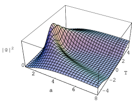
Figure 1: The figures show the square of the wave function (36) and its contourplot.

In figure 1 we have plotted the square of the wave function and its contourplot for typical numerical values of the parameters. As this figure shows, at $T=0$, the wave function has a dominant peak in the vicinity of some non-zero value of $a$. This means that the wave function predicts the emergence of the universe from a state corresponding to its dominant peak. As time progresses, the wave packet begins to propagate in the $a$-direction, its width becoming wider and its peak moving with a group velocity towards the greater values of scale factor. The wave packet disperses as time passes, the minimum width being attained at $T=0$. As in the case of the free particle in quantum mechanics, the more localized the initial state at $T=0$, the more rapidly the wave packet disperses. Therefore, the quantum effects make themselves felt only for small enough $T$ corresponding to small $a$, as expected and the wave function predicts that the universe will assume states with larger $a$ in its late time evolution. Now, having the above expression for the wave function of the universe, we are going to deal with the question of the recovery of the classical solutions, in other words, how can the Wheeler-DeWitt wave functions predict a classical universe. In this approach, as we have done above, one usually constructs a coherent wave packet with good asymptotic behavior in the minisuperspace, peaking in the vicinity of the classical trajectory. On the other hand, to show the correlations between classical and quantum pattern, following the many-worlds interpretation of quantum mechanics [9], one may calculate the time dependence of the expectation value of a dynamical variable $q$ as

$$<q>(t)=\frac{<\Psi|q|\Psi>}{<\Psi|\Psi>}.$$ (37)

Following this approach, we may write the expectation value for the scale factor as

$$<a>(T)=\frac{\int_{0}^{\infty}\Psi^{*}(a,T)a\Psi(a,T)da}{\int_{0}^{\infty}\Psi^{*}(a,T)\Psi(a,T)da},$$ (38)

which yields

$$<a>(T)\sim\frac{T^{2}+\gamma^{2}+3\gamma}{T^{2}+\gamma^{2}+12\gamma}e^{\frac{T^{2}+\gamma^{2}}{8\gamma}}.$$ (39)

It is important to classify the nature of the quantum model as concerns the presence or absence of singularities. For the wave function (36), the expectation value (39) of scale factor never vanishes, showing that these states are nonsingular. Indeed, the expression (39) represents a bouncing universe with no singularity where its late time behavior coincides to the late time behavior of the classical solution. This means that the quantum structure which we have constructed has a good correlation with its classical counterpart.

The issue of the correlation between classical and quantum schemes may be addressed from another point of view. It is known that the results obtained by using the many-world interpretation agree with those that can be obtained using the ontological interpretation of quantum mechanics [10]. In Bohmian interpretation, the wave function is written as $\Psi(a,T)=\Omega(a,T)e^{iS(a,T)}$, where $\Omega(a,T)$ and $S(a,T)$ are real functions, which using the expression (36), a simple algebra gives them as

$$\Omega(a,T)={\cal N}\left(\gamma^{2}+T^{2}\right)^{-3/4}\exp\left(-3\gamma\frac{\ln^{2}a}{\gamma^{2}+T^{2}}\right)\ln a,$$ (40)

$$S(a,T)=\frac{3}{2}\arctan\frac{T}{\gamma}-\frac{3T\ln^{2}a}{\gamma^{2}+T^{2}}.$$ (41)

In this interpretation the classical trajectories, which determine the behavior of the scale facto is given by $P_{a}=\frac{\partial S}{\partial a}$, where by means of the relation (4) reads

$$\frac{1}{a}\frac{da}{dT}=\frac{T}{\gamma^{2}+T^{2}}\ln a,$$ (42)

which, after integration we get

$$a(T)=a_{0}e^{\sqrt{\gamma^{2}+T^{2}}}.$$ (43)

This solution has the same behavior as the expectation values computed in (39) and like that is free of singularity. figure 2 shows the behavior of the classical scale factor (21), the quantum mechanical expectation value of the scale factor (39) and its Bohmian version (43) versus time for some typical numerical values of the parameters. We see that instead of two separate classical solutions, the quantum models predict a bouncing universe in which the universe decreases its size, reaches a minimum and then expands forever. The origin of the singularity avoidance may be understood by the existence of the quantum potential which corrects the classical equations of motion. According to the Bohm-de Broglie interpretation of quantum mechanics and also its usage in quantum cosmology, upon using the polar form of the wave function $\Psi(a,T)=\Omega(a,T)e^{iS(a,T)}$, in the corresponding wave equation, we arrive at the modified Hamilton-Jacobi equation as

$${\cal H}\left(q_{i},P_{i}=\frac{\partial S}{\partial q_{i}}\right)+{\cal Q}=0,$$ (44)

where $P_{i}$ are the momentum conjugate to the dynamical variables $q_{i}$ and ${\cal Q}$ is the quantum potential. For the wave equation (28) this procedure leads

$$-\frac{1}{12a}\left(\frac{\partial S}{\partial a}\right)^{2}+\frac{1}{a^{3}}\left(\frac{\partial S}{\partial T}\right)-3ka+{\cal Q}=0,$$ (45)

in which the quantum potential is defined as

$${\cal Q}=\frac{1}{12a\Omega}\frac{\partial^{2}\Omega}{\partial a^{2}}+\frac{1}{12a^{2}\Omega}\frac{\partial\Omega}{\partial a}.$$ (46)

Now, inserting the relation (43) in (46), we can find the quantum potential in terms of the scale factor as

$${\cal Q}\sim\frac{1}{a^{3}\ln^{2}(\frac{a}{a_{0}})}.$$ (47)

As this relation shows, the potential goes to zero for the large values of the scale factor. This behavior is expected, since in this regime the quantum effects can be neglected and the universe evolves classically. On the other hand, for the small values of the scale factor the potential takes a large magnitude and the quantum mechanical considerations come into the scenario. This is where the quantum potential can produce a huge repulsive force, which may be interpreted as being responsible of the avoidance of singularity.

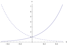
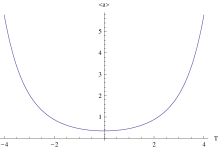
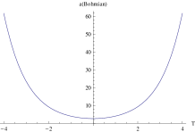
Figure 2: From left to right: The classical scale factors (21), the expectation value (39) and the Bohmian value (43).

$\bullet$ The closed universe: $k=1$. Equation (30) in this case admits the following solutions in terms of the modified Bessel functions

$$\psi_{E}(a)=c_{1}K_{i\sqrt{3E}}\left(3a^{2}\right)+c_{2}I_{i\sqrt{3E}}\left(3a^{2}\right).$$ (48)

We impose the boundary condition $\lim_{x\rightarrow\infty}\psi(x)=0$ on the wave function which restricts us to consider the modified Bessel function $K$ as solution. Thus the eigenfunctions of the SWD equation take the form

$$\Psi_{E}(a,T)=e^{iET}K_{i\sqrt{3E}}\left(3a^{2}\right),$$ (49)

which their superposition gives the general solution as

$$\Psi(a,T)=\int_{0}^{\infty}\frac{2}{3}\nu C(\nu)e^{\frac{1}{3}i\nu^{2}T}K_{i\nu}\left(3a^{2}\right)d\nu,$$ (50)

where $\nu=\sqrt{3E}$. Since the function $K_{i\nu}(z)$ decreases when $\nu$ grows, thus the small $\nu$’s have dominate contribution to the above integral. This allows us to use the approximation $\nu^{2}/3\sim\nu$. Therefore, with the choice of the weight factor as $C(\nu)=\frac{3}{2}e^{\gamma\nu}$ we get

$$\Psi(a,T)=\int_{0}^{\infty}\nu e^{i(T-i\gamma)\nu}K_{i\nu}\left(3a^{2}\right)d\nu.$$ (51)

Now, by using the equalities [11]

$$\int_{0}^{\infty}\cos(\beta\nu)K_{i\nu}(\alpha)d\nu=\frac{\pi}{2}e^{-\alpha\cosh\beta},\hskip 8.5359pt\int_{0}^{\infty}\nu\sin(\beta\nu)K_{i\nu}(\alpha)d\nu=\frac{\pi}{2}\alpha\sinh\beta e^{-\alpha\cosh\beta},$$ (52)

for $\alpha>0$ and $|\mbox{Im}\beta|<\frac{\pi}{2}$, we can evaluate the integral in (51) to achieve the following analytic form for the wave function

$$\Psi(a,T)={\cal N}\left[1+3a^{2}\sin\left(\gamma+iT\right)\right]e^{-3a^{2}\cos\left(\gamma+iT\right)},$$ (53)

where again ${\cal N}$ is a numerical factor and $\gamma$ should be chosen as $|\gamma|<\frac{\pi}{2}$.

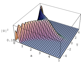
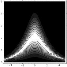
Figure 3: The figures show the square of the wave function (53) and its contourplot.

In figure 3 the wave function and its contourplot is plotted. This figure shows the universe expands and after reaches a maximum recollapses. It is clear that the two phases of cosmic evolution are connected to each other without meeting any kind of singularity. Now, with the help of the definition (37) we can evaluate the expectation value of the scale factor when the corresponding quantum universe is in the state (53). This calculation results

$$<a>(T)=\cosh^{-1/2}T\times$$

$$\frac{8\left(e^{T}+e^{3T}+e^{5T}\right)+\left(1+e^{2T}\right)^{3}\cos\gamma+4e^{T}\left(1+e^{4T}\right)\cos 2\gamma-\left(1+3e^{2T}+3e^{4T}+e^{6T}\right)\cos 3\gamma}{11e^{T}+16e^{3T}+11e^{5T}+\left(1+e^{2T}\right)^{3}\cos\gamma+2\left(4+5e^{2T}+4e^{4T}\right)\cos 2\gamma-\left(1+3e^{2T}+3e^{4T}+e^{6T}\right)\cos 3\gamma},$$ (54)

where is plotted in figure 4. Also, to extract the Bohmian trajectories of this model we may write the wave function (53) as $\Psi(a,T)=\Omega(a,T)e^{iS(a,T)}$ in which

$$\Omega(a,T)=\left[1+9a^{4}\left(\sin^{2}\gamma\cosh^{2}T+\cos^{2}\gamma\sinh^{2}T\right)+6a^{2}\sin^{2}\gamma\cosh^{2}T\right]^{1/2}e^{-3a^{2}\cos\gamma\cosh T},$$ (55)

and

$$S(a,T)=3a^{2}\sin\gamma\sinh T+\arctan\frac{3a^{2}\cos\gamma\sinh T}{1+3a^{2}\sin\gamma\cosh T}.$$ (56)

Substitution of the relation (56) in $P_{a}=\frac{\partial S}{\partial a}$ and using of the definition $P_{a}$ in (4), we obtain

$$\frac{da}{dT}=-\frac{a^{3}\sinh T\left[\cos\gamma+\sin\gamma-\frac{9}{2}a^{4}\left(\cos 2\gamma-\cosh 2T\right)\sin\gamma+6a^{2}\cosh T\sin^{2}\gamma\right]}{1-\frac{9}{2}a^{4}\left(\cos 2\gamma-\cosh 2T\right)+6a^{2}\cosh T\sin\gamma}.$$ (57)

This equation does not seem to have analytical solution. However, in figure 4, employing numerical methods, we have shown the qualitative behavior of $a(T)$ for typical values of the parameters and initial conditions. As is clear from the figure, the scale factor repeats its expansion and contraction behavior as its expectation value also shown in this figure. We see that the quantization of the closed FRW cosmology predicts an evolution pattern for the corresponding universe in completely agreement with its classical dynamics which means that there is a good correlation between the classical and quantum models in this case as well.

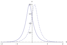
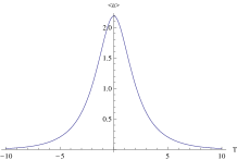
Figure 4: From left to right: The classical scale factors (24), the expectation value (3) and the Bohmian trajectory obtained from (57).

$\bullet$ The open universe: $k=-1$. The solutions to the equation (30) with $k=-1$ read as

$$\psi_{E}(a)=c_{1}J_{i\sqrt{3E}}(3a^{2})+c_{2}Y_{i\sqrt{3E}}(3a^{2}),$$ (58)

where $J$ and $Y$ are the Bessel functions. Removing the function $Y$ from the solutions because of applying the same boundary condition as in the closed case, we are led to the following eigenfunctions

$$\Psi_{E}(a,T)=e^{iET}J_{i\sqrt{3E}}(3a^{2}).$$ (59)

We may now write the general solutions to the SWD equation as a superposition of the above eigenfunctions

$$\Psi(a,T)=\int_{0}^{\infty}C(E)e^{iET}J_{i\sqrt{3E}}(3a^{2})dE.$$ (60)

Unfortunately, unlike the previous two cases, it is not possible to find an analytical closed form for the wave function in the case of the open universe. Therefore, we should rely on the numerical methods by using of the shifted Gaussian weight function $C(E)=e^{-\gamma(E-\sigma)^{2}}$. In figure 5 we have plotted the square of the wave function and its contourplot. The discussions on the comparison between quantum cosmological solutions and their corresponding form from the classical formalism are the same as previous models, namely the flat and closed models. Similar discussion as above would be applicable to this case as well.

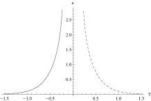
Figure 5: From left to right: The classical scale factors (27), the square of the wave function (60) and its contourplot.

4 Summary

In this letter we took a look at the problem of time in the framework of a scalar field cosmology. To do this, we have examined a canonical transformation $(\phi,P_{\phi})\rightarrow(T,P_{T})$ on the scalar field sector of the action which turns out to correspond to a specific choice of time parameter. In terms of this time parameter, we have solved the classical field equations in the cases of the flat, closed and open FRW universe and obtained the analytical expressions for the corresponding scale factors. As for the quantum version of these models, the use of the above mentioned canonical transformation allowed us to obtain a SWD equation in which the variable $T$ plays the role of time parameter. In the cases of the flat and closed FRW models, we obtained exact solutions of the SWD equation and for the open model the wave function is represented numerically. The wave functions of the corresponding universes consist of some branches where each may be interpreted as part of the classical trajectories. We saw that since the peaks of the wave functions follow the classical trajectories, there seems to be good correlation between the corresponding classical and quantum cosmology.

One of the main features of the quantum solutions in our presented model is that the singular region of the classical cosmologies is replaced by a bouncing period. In such a behavior which is shown in figures 1-5 the scale factor bounces (falls) from the contraction (expansion) to its expansion (contraction) eras. In addition to singularity avoidance, the appearance of bounce in the quantum model is also interesting in its nature due to prediction of a minimal size for the corresponding universe. We know the idea of existence of a minimal length in nature is supported by almost all candidates of quantum gravity. In this sense our results are qualitatively comparable with other works in which different quantization schemes are considered. We may name some of such works, for instance, as:

$\bullet$ In [12], using the polymer quantization method of a $k=0$ FRW model, the volume of the corresponding universe is obtained as $\sqrt{\gamma^{2}\lambda^{2}+9t^{2}}$, where $\gamma$ is the Barbero-Immirzi parameter and $\lambda$ is a parameter associated to the fundamental granularity of quantum geometry.

$\bullet$ In [13], using a gauge-fixed Lagrangian to quantize a perfect fluid FRW cosmology, a bouncing scale factor $(\gamma^{2}+t^{2})^{\frac{1}{3(\omega+1)}}$, for ordinary perfect fluid and a falling one $[\gamma^{2}+(t_{0}-t)^{2}]^{-\frac{1}{3(\omega+1)}}$ for phantom perfect fluid is obtained, where $\gamma$ is an arbitrary positive constant and $\omega$ is the equation of state parameter of the perfect fluid.

$\bullet$ In [14], a perfect fluid FRW cosmology is quantized with the use of the Schutz’ representation of the perfect fluid which is shown may lead to an identification to a time parameter. The bouncing expression such as $[\frac{9(1-\omega)^{4}}{\gamma^{2}}t^{2}+1]^{\frac{1}{3(1-\omega)}}$ is obtained for the scale factor in this model.

$\bullet$ In [15] several bouncing solutions of various cosmological models are investigated and the mechanisms behind the bounce are discussed.
Acknowledgements
The author is grateful to the research council of IAU, Chalous Branch for financial support.

References

-
[1]
B.S. DeWitt, Phys. Rev. 160 (1967) 1113
B.S. DeWitt, Phys. Rev. 162 (1967) 1195
B.S. DeWitt, Phys. Rev. 162 (1967) 1239 -
[2]
C.W. Misner, Phys. Rev. 186 (1969) 1319
A. Vilenkin, Phys. Lett. B 117 (1982) 25
A. Vilenkin, Phys. Rev. D 27 (1983) 2848
J.B. Hartle and S.W. Hawking, Phys. Rev. D 28 (1983) 2960
S.W. Hawking, Nucl. Phys. B 239 (1984) 257
J.J. Halliwell and S.W. Hawking, Phys. Rev. D 31 (1985) 1777
A. Vilenkin, Phys. Rev. D 33 (1986) 3560
A. Vilenkin, Phys. Rev. D 37 (1988) 888
A. Vilenkin, Phys. Rev. D 50 (1994) 2581 -
[3]
M. Bojowald, Quantum Cosmology: A Fundamental Description of the Universe
(Springer, New York, 2011)
C. Kiefer, Quantum Gravity (Oxford University Press, New York, 2007)
G. Esposito, An introduction to quantum gravity (arXiv: 1108.3269 [hep-th]) -
[4]
F. Amemiya and T. Koike, Phys. Rev. D 80 (2009) 103507
P. Dzierzak, P. Małkiewicz and W. Piechocki, Phys. Rev. D 80 (2009) 104001
P. Małkiewicz and W. Piechocki, Class. Quantum Grav. 27 (2010) 225018
A. Kreienbuehl, Phys. Rev. D 79 (2009) 123509
B. Vakili and H.R. Sepangi, Ann. Phys. 323 (2008) 548
W.F. Blyth and C.J. Isham, Phys. Rev. D 11 (1975) 768 - [5] C.J. Isham, Canonical Quantum Gravity and the Problem of Time (arXiv: gr-qc/9210011)
-
[6]
J.D. Brown and K.V. Kuchař, Phys. Rev. D 51 (1995) 5600
M. Castagnino, Phys. Rev. D 39 (1988) 2216
J. Greensite, Nucl. Phys. B 342 (1990) 409
C.J. Isham and J. Butterfield, On the Emergence of Time in Quantum Gravity (arXiv: gr-qc/9901024)
R.M. Wald, Phys. Rev. D 48 (1993) R2377
S. Sawayama, Problem of the time and static restriction in quantum gravity (arXiv: 0705.2916 [gr-qc])
C. Kiefer, Does time exist in quantum gravity? (arXiv: 0909.3767 [gr-qc])
E. Anderson, Problem of Time in Quantum Gravity (arXiv: 1206.2403 [gr-qc])
A. Davidson and B. Yellin, Restoring Time Dependence into Quantum Cosmology (arXiv: 1206.0830 [gr-qc]) - [7] H. Farajollahi, M. Farhoudi and H. Shojaie, Int. J. Theor.Phys. 49 (2010) 2558
-
[8]
A. Anderson, Ann. Phys. 232 (1994) 292 (arXiv:
hep-th/9305054)
M. Błaszak and Z. Domański, Canonical transformations in quantum mechanics (arXiv: 1208.2835 [math-ph]) - [9] F.J. Tipler, Phys. Rep. 137 (1986) 231
-
[10]
D. Bohm, Phys. Rev. 85 (1952) 166
D. Bohm, Phys. Rev. 85 (1952) 180
P.R. Holland, The Quantum Theory of Motion: An Account of the de Broglie-Bohm Interpretation of Quantum Mechanics (Cambridge University Press, Cambridge, 1993)
F.T. Falciano and N. Pinto-Neto, Phys. Rev. D 79 023507
A. Shojai and F. Shojai, Europhys. Lett. 71 (2005) 886 - [11] I.S. Gradshteyn, I.M. Ryzhik, A. Jeffrey and D. Zwillinger, Table of Integrals, Series and Products (Academic Press, San Diego, 2000)
- [12] A. Corichi and T. Vukašinac, Phys. Rev. D 86 (2012) 064019 (arXiv: 1202.1846 [gr-qc])
- [13] B. Vakili, Phys. Rev. D 83 (2011) 103505 (arXiv: 1104.1163 [gr-qc])
-
[14]
F.G. Alvarenga, J.C. Fabris, N.A. Lemos and G.A.
Monerat, Gen. Rel. Grav. 34 (2002) 651 (arXiv:
gr-qc/0106051)
B. Vakili, Phys. Lett. B 688 (2010) 129 (arXiv: 1004.0306 [gr-qc]) - [15] M. Novello and S.E.P. Bergliaffa, Phys. Rept. 463 (2008) 127 (arXiv: 0802.1634 [astro-ph])