The nature of the unresolved extragalactic soft CXB

Abstract

In this paper we investigate the power spectrum of the unresolved 0.5-2 keV CXB with deep Chandra 4 Ms observations in the CDFS. We measured a signal which, on scales $>$30$\arcsec$, is significantly higher than the Shot-Noise and is increasing with the angular scale. We interpreted this signal as the joint contribution of clustered undetected sources like AGN, Galaxies and Inter-Galactic-Medium (IGM). The power of unresolved cosmic sources fluctuations accounts for $\sim$12% of the 0.5-2 keV extragalactic CXB. Overall, our modeling predicts that $\sim$20% of the unresolved CXB flux is made by low luminosity AGN, $\sim$25% by galaxies and $\sim$55% by the IGM (Inter Galactic Medium). We do not find any direct evidence of the so called Warm Hot Intergalactic Medium (i.e. matter with 10⁵K$<$T$<$10⁷K and density contrast $\delta<$1000), but we estimated that it could produce about 1/7 of the unresolved CXB.

We placed an upper limit to the space density of postulated X-ray-emitting early black hole at z$>$7.5 and compared it with SMBH evolution models.

1 Introduction

The Cosmic X-ray Background (CXB) is the result of a multitude of energetic phenomena occurring in the Universe since the epoch of the formation of the first galaxies. Its nature has been investigated in the last 50 years with several telescopes but only in the 80’s it became clear that its main contributors are AGN (Setti & Woltjer, 1989). Later it has been found that also galaxies, galaxy clusters, large scale structures and diffuse hot gas in the Milky Way are sources contributing to the CXB (Fabian & Barcons, 1992).
With the launch of ROSAT, Chandra and XMM-Newton, the knowledge about the nature of sources contributing to the flux of the CXB became suddenly clear. Deep surveys like the Chandra Deep Field South (CDFS, Giacconi et al., 2001; Luo et al., 2008; Xue et al., 2011) and North (CDFN, Brandt et al., 2001), and the Lockman Hole (Brunner et al., 2008) have almost conclusively resolved the problem of the CXB below 10 keV. In fact at the flux limits of Chandra and XMM-Newton, about 90-95$\%$ (Bauer et al., 2004; Moretti et al., 2003; Lehmer et al., 2012) of the 0.5-2 keV CXB flux has been resolved into point and extended sources.
CXB synthesis models (see e.g. Treister & Urry, 2006; Gilli et al., 2007) predict that at fluxes fainter that the current limits, the AGN source counts progressively flatten and then galaxies become the more abundant sources.
Galaxies emerge as the dominant population at faint 0.5-2 keV fluxes, with break-even point at around $\sim$10^-17 erg cm^-2 s^-1(see also Lehmer et al., 2007; Xue et al., 2011; Lehmer et al., 2012) and can make up for a sizable fraction of the X-ray background (9-16%; Ranalli et al. 2005). The contribution from galaxy clusters, down to a mass limit of $\sim$10¹³ M_⊙, has been estimated to be of the order of $\sim$10% of the total 0.5-2 keV CXB (Gilli et al., 1999; Lemze et al., 2009).
Several authors studied the clustering properties of the CXB to unveil the nature of the sources producing its flux and their properties (Martin-Mirones et al., 1991; Wu & Anderson, 1992; Sołtan & Hasinger, 1994; Barcons et al., 1998). The most used technique is that of the two-point autocorrelation function of the surface brightness of the CXB. While at the time of HEAO-1 the task was to determine what was the contribution of QSO to the CXB, after ROSAT most of the investigations in this field have been performed to unveil signatures of the Warm Hot Intergalactic Medium (Sołtan et al., 2002; Sołtan, 2006; Galeazzi et al., 2009) and to test Cosmological models (Diego et al., 2003). This kind of studies is therefore extremely powerful to study population of sources which are beyond the resolving and detection capabilities of instruments.

In the GOODS fields, Hickox & Markevitch (2006, 2007) have shown that, after excising detected point and extended sources plus faint HST detected galaxies, the spectrum of the soft CXB was still showing a signal in the 0.5-2 keV band. While a large amount of it could be attributed to a local component (Solar Wind Charge Exchange and Milky Way thermal emission), they have shown that below 1 keV the fraction of the resolved CXB is not sensitive to the removal of HST galaxies, thus arguing for a purely diffuse nature of the unresolved CXB. In the 1-2 keV band they have shown that, by removing HST sources areas from the analysis, the fraction of unresolved CXB drops by $\sim$50%. This means that a large fraction of the unresolved 1-2 keV CXB flux could be produced in faint undetected galaxies (active or non-active). Moreover, they speculated that a large fraction of the unresolved CXB may be due to faint 3.6$\mu$m IRAC sources, suggesting that high-z or absorbed sources could produce a large part of such a radiation. According to their estimate, the remaining fraction of the CXB (i.e. 2-3% of the 0.5-2 keV CXB) remains consistent with the prediction of Warm Hot Intracluster Medium (WHIM) intensity from hydrodynamical simulations (see e.g Cen & Ostriker, 1999; Ursino & Galeazzi, 2006; Roncarelli et al., 2006, 2012).
In the local Universe about 30-40% of the baryons are missing with respect to what is measured at z$\sim$3 (Fukugita et al., 1998). Simulations predict that most of these baryons got shock-heated and at z$\lesssim$1 they should have a temperature of the order 10⁵-10⁷ K and therefore emit thermal X-rays (Cen & Ostriker, 1999). Controversial evidences on the properties of such a medium have been published so far (see e.g., Nicastro et al., 2005; Kaastra et al., 2006; Fang et al., 2010; Shull et al., 2011). Though with very low surface brightness, the WHIM can be distinguished from other kinds of diffuse emissions on the basis of its clustering properties (Ursino & Galeazzi, 2006). In fact, its emission follows that of clusters and filaments and peaks at low redshift (z$\sim$0.5), thus showing a typical feature in the angular clustering of unresolved CXB fluctuations. However, WHIM is not the only expected component of the unresolved CXB arising from thermal emission of the Inter Galactic Medium (IGM). X-ray surveys in the local Universe revealed X-ray emission from local galaxy groups down to masses of the order of 10¹² M_⊙ (see e.g. Eckmiller et al., 2011). Since the intensity of the X-ray emission of galaxy groups scales with their mass, a large amount of them has not been detected at moderately high-z. Therefore we also expect a contribution to the overall signal from medium to low mass-groups at z$>$0.2-0.3.
Concerning the unresolved extragalactic CXB, it is difficult to distinguish its components with a simple spectral analysis mostly because of the poor energy resolution of X-ray sensitive CCDs (i.e. $\sim$130 eV, for ACIS-I at 1.5 keV). However, cosmological sources leave a unique imprint in the power spectrum (PS) of the anisotropies of the fluctuations of the unresolved CXB in a way that is related to their clustering and volume emissivity properties.
The unresolved CXB contains information about all those sources that have not been detected at the deepest fluxes reachable by deep surveys. Moreover, the amplitude of the PS is not only sensitive to the luminosity density of those sources, but it also provides information about their bias.

In this paper we study the power spectrum of the unresolved 0.5-2 keV CXB with the 4Ms CDFS data, the deepest X-ray observation ever performed to date. We model the anisotropies of unresolved CXB with the state-of-the art results on galaxy and AGN evolution models and observations as well as with modern hydrodynamical cosmological simulations.
Throughout this paper we will adopt a concordance $\Lambda$-CDM cosmology with $\Omega_{m}$=0.3, $\Omega_{\Lambda}$=0.7, H₀=70 h km/s/Mpc and $\sigma_{8}$=0.83. Unless otherwise stated, errors are quoted at 1$\sigma$ level and fluxes refer to the 0.5–2 keV band. We used as reference cumulative 0.5-2 keV CXB flux the recent estimates of Lehmer et al. (2012), S_CXB(0.5-2)=8.15$\pm{0.58}\times$10^-12 erg cm^-2 s^-1 deg^-2.

2 Dataset

For the purposes of this work we used the 4 Ms Chandra exposure on the CDFS (Xue et al., 2011). This is the deepest Chandra observation ever performed and reaches a point source flux limit of $\sim$10^-17 erg cm^-2 s^-1. A detailed description of the data reduction and catalogue production is given in Xue et al. (2011). In order to improve the sensitivity on extended sources, we also used the 3 Ms XMM-Newton exposure in the same field (Ranalli et al., 2012). Since the scope of this paper is to measure the angular PS (see next section) of the purely diffuse, unresolved CXB, we masked the Chandra data from all the point sources detected by Xue et al. (2011). The combination of the Chandra and XMM-Newton observations allowed us to remove, with unprecedented sensitivity, also extended sources down to 0.5-2 keV fluxes of 2$\times$10^-16 erg cm^-2 s^-1  (Finoguenov et al. , private communication). In order to employ the best-PSF area, we limited our analysis to the inner 5$\arcmin$ from the exposure weighted mean optical axis ($\alpha$=03:32:27.316, $\delta$=-27:48:50.36). Point sources have been masked with circular regions of 5$\arcmin\arcmin$ radius (which is large enough to mask $>$99% of the source flux at every off-axis angle investigated here) and extended sources have been masked out to R₂₀₀ (i.e. radius within which the matter overdensity is $>$200). In this way the remaining counts on the detector are made, with good approximation, by particle background and purely diffuse cosmic background only. With such a masking our image contains 163940 counts, with an average occupation number of 1.7 cts/pix. The total investigated masked area (80.3 arcmin²) is shown in Fig. 1 together with the raw image of the same region. The source masking removes a fraction of the useful area of about $\sim$25% and therefore the source-free area is of the order of 60 arcmin². In principle the evaluation of the PS should not change if we increase the size of the mask. However by increasing the mask size we would run into an over-masking problem that would bias the estimate of the PS. If the masking were larger than $\sim$30%-40% of the active pixels then the PS analysis would have been biased by the mask (Kashlinsky et al., 2012). A smaller size of the mask would increase the overall power since it would be polluted by power from cluster outskirts and PSF tails of detected sources. In order to improve the signal to noise ratio of the weak signal we are looking for, we applied a careful filtering of the background. We have additionally filtered the events files provided by the CXC from particle flares by using the ciao routine $lc\_clean$, which performs a 3$\sigma$ clipping of the background light-curve. Such a technique is more sensitive than the classical procedures adopted in standard pipelines. In order to reduce the noise introduced by low-count statistics, images were binned in pixels of 1.5$\arcsec$ size. Images have been produced in the 0.5-2 keV energy range, where Chandra has the largest collecting area and detector efficiency.

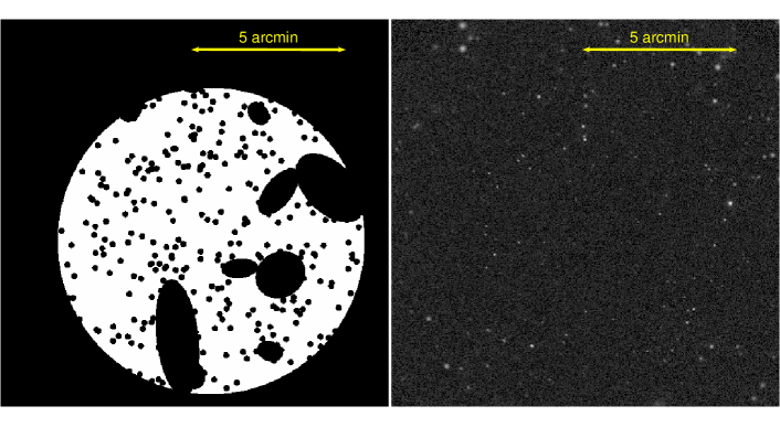
Figure 1: $Left:$The mask adopted for the ACF analysis in the observations of the CDFS. The white area is the resulting source-free area. $Right:$ 0.5-2 keV image of the same area smoothed with a Gaussian filter with 3$\arcsec$ width.

3 Evaluation of the power spectrum

In order to estimate the power spectrum we adopt the method described in Arevalo et al. (2012) and Churazov et al. (2011) that has been developed with the purpose of estimating the PS of 2D images with gaps. Here we give a brief description of the technique used to evaluate the PS, but we refer the reader to Arevalo et al. (2012) for a more comprehensive description.
The first step is to derive the fluctuation field at any given angular scale $\theta$, from which we derive a low-resolution PS by using a Mexican-Hat (MH) filter, $F(x)=[1-\frac{x^{2}}{\theta^{2}}]e^{-\frac{x^{2}}{2\theta^{2}}}$.
The goal is to single out fluctuations at any given angular scale and then compute the variance of the fluctuation field image, $\delta_{S}^{2}(k)$. Our map has gaps introduced by features in the exposure maps and by the mask. The mask (M) is an image having value M=0 in the region of excised sources and M=1 elsewhere. The method corrects for gaps by representing the MH filter as a difference between two Gaussian filters with slightly different widths, convolving the image and the mask with these filters and dividing the results before calculating the final filtered images. It has been shown (Arevalo et al., 2012) with numerical simulations that this method efficiently takes into account data masking also when a large fraction of the field is masked and, independently from the mask shape, the normalization and the shape of the PS is accurately estimated. At any given frequency $k$=1/$\theta$, we estimated the PS of the fluctuation field as follows:

We define the fluctuation image at the scale $\theta$ as:

$$I_{\theta}=M\times\left[\frac{G_{\theta_{1}}\circ(I)}{G_{\theta_{1}}\circ M}-\frac{G_{\theta_{2}}\circ(I)}{G_{\theta_{2}}\circ M}\right].$$ (1)

where (G${}_{\theta_{1}}\circ$ I, G${}_{\theta_{2}}\circ$ I) represent the count-rate image (I) convolved with a gaussian filters with widths $\theta_{1,2}$ (G) and M is the mask. The width of the filter is chosen as $\theta_{1}=\theta\sqrt{1+\epsilon}$ and $\theta_{2}=\theta/\sqrt{1+\epsilon}$, where $\epsilon<<$1. In this way the value in the brackets of eq.1 is dominated by fluctuations at the scale $\sim\theta$.
Arevalo et al. (2012) demonstrated that PS of the fluctuation field at the frequency $k$=1/$\theta$ (P₂(k)) is related to the variance of image via:

$$P_{2}(k)=\frac{1}{\epsilon^{2}\pi k^{2}}\sigma^{2}(I_{\theta})=<|\delta_{S}(k)|^{2}>.$$ (2)

In this work we used $\epsilon=$0.1, however a different value of $\epsilon$ does not change the estimate of the PS, provided that $\epsilon<<$1. Note that in the calculation of the variance we have made no assumption on the distribution of the fluctuation amplitude, thus the method works also in the Poisson regime. This method is equivalent to the classical Fourier analysis; the only difference is that this treatment of the gaps and choice of the filters allow us to retrieve the underlying power-spectrum regardless of the shape of the mask. Unless otherwise stated, errors are given at the $1\sigma$ level. In Fourier analysis, the uncertainty on power estimate is solely related to the accuracy with which one can estimate the variance. At every frequency, this depends on the number of independent elements in the Fourier space, and the intrinsic dispersion of the data. In our analysis, since we adopt a broad filter, we need to define, at every frequency $k$, the mean number of real Fourier elements used to evaluate the amplitude of the fluctuations $<N_{k}>$. In principle the uncertainties can be approximated with $\sigma_{P}(k)\approx\,P_{2}(k)/\sqrt{0.5<N_{k}>}$. Following the extensive description of Arevalo et al. (2012), within our formulation errors are computed with:

$$\sigma_{P}(k)=\frac{\sqrt{\int_{q}(P(k)\,F_{qx}^{2}dq}}{F^{2}_{kx}}\frac{N}{N_{M=1}},$$ (3)

where F_kx is the Fourier transform of the filter, N is total number of pixels and N_M=1 is the number of unmasked pixels.
This filter-weigthed expected uncertainties is what we plot as error bars.

Power spectrum points measured in this way are partially dependent on their neighbor frequencies as a result of the finite width of the power filter. Therefore, points can only be considered independent if they are measured at spatial scales that are sufficiently separated. In our case, where we used a factor of 2 separation in angular scale, it is appropriate to use PS estimates and errors as independent points in the usual fitting methods.

4 Results

4.1 Baseline method

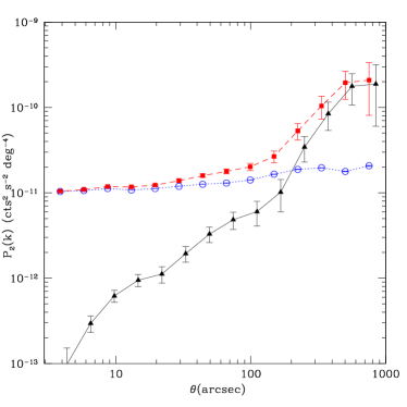
Figure 2: $Red~{}squares:$ the raw PS of the source-masked fluctuations of the CXB as a function of the angular scale. $Blue~{}open~{}circles:$ the (A-B)/2 PS. $Black~{}Triangles:$ The resulting Cosmic PS after subtracting the ”spurious” power. $Black~{}symbols$ are artificially shifted for sake of clarity.

The power spectrum estimated with the technique described is Sect. 3 is shown in Fig. 2. We computed the probability that the observed data could be produced by a statistical fluctuation of a zero power signal by using a simple $\chi^{2}$ test. We obtained a value of $\chi^{2}$=140 corresponding to a $>$10$\sigma$ significance with respect to zero power. The high frequency part is dominated by a white noise component, while the signal increases towards lower frequencies (i.e. large scales). In Chandra images a large fraction of the fluctuation can be attributed to Poisson noise due to the low-count statistics.

We estimated $P_{noise}$ directly from the data by using the A-B technique (Kashlinsky et al., 2005). For every pointing we sorted the events in order of time arrival and created two images, one including even events (A), and the other with odd events (B). We have then mosaiced all the A and B images. In this way we have two identical images with half the photons with respect to the full dataset, having both the same exposure, thus containing the same information on the signal but with their own noise. Any systematic errors should be manifested very similarly in the A and B images, and thus the (A-B)/2 difference images provide a useful means of characterizing the random (noise) properties of the data sets. The PS of the difference image (A-B)/2 is therefore nothing else than the PS of fluctuations due to Poisson noise. Source variability does not affect this procedure since the sampling of their light curve does not change significantly: the gap between two consecutive events is of the order of the read-out time of the detector, which is much shorter than the typical variability of X-ray sources. In Fig. 2 we show the PS of the Poisson noise compared with the PS of the raw image. As expected, the Poisson Noise shows a flat (white noise) spectrum. Throughout this paper we assume that both particle and galactic background contribute only to the Poisson noise since their flux is expected to be homogeneous at the scales sampled by this investigation. The total cosmic PS (P_2,CXB) is therefore obtained with:

$$P_{2,CXB}=P_{2,tot}-P_{2,(A-B)/2}.$$ (4)

The estimated P_2,CXB is plotted in Fig. 2. In the angular range sample here (3$\arcsec<\theta<1000\arcsec$), the power increases with the scale, getting close to zero at smallest scale. The errors on P_2,CXB have been obtained by propagating the errors of P_2,tot and P_2,(A-B)/2.

5 Modeling the CXB anisotropies

In order to interpret the cosmic signal measured in the PS of the CXB, we used population synthesis models and recent observational results to predict amplitude and shape of its components. We want to test the assumption that the total observed fluctuations can be reproduced by a simple 3 source class model. Our hypothesis is that the amplitude and the shape of the PS are produced by: Shot Noise from individual undetected AGN and galaxies within the instrument beam (discrete source counts), clustering of galaxies and AGN below the limiting flux, clustering of undetected diffuse hot cosmological gas in large scale structures (IGM, i.e. undetected groups and WHIM filaments). We then test the statistical robustness of our hypothesis with $\chi^{2}$ test where every component is considered as a parameter. In addition we provide an upper limit for the still undetected high-z sources. We assumed that, on the angular scales investigated here, fluctuations from the Milky Way diffuse emission does not contribute to the PS, i.e. this emission can be described as a constant flux on the detector and therefore contributing to the Poisson noise only. This hypothesis is supported by the PS measurements of the soft CXB with ROSAT (Śliwa et al., 2001) that shows that the Galaxy produces signal only for the smallest harmonics of the PS. Moreover, cosmological sources (AGN, Galaxies and IGM) partially share the same environment, thus we include in the model a cross power term to model the amplification of fluctuations produced by their cross-correlation. In summary, the CXB PS can be modeled as:

$$\begin{split}P&{}_{2,CXB}(k)=P_{2,SN}(k)+P_{2,AGN}(k)+\\ &P_{2,GAL}(k)+P_{2,IGM}(k)+P_{2,A,G,I}(k),\end{split}$$ (5)

where $P_{2,SN}(k),P_{2,AGN}(k),P_{2,GAL}(k)$ and $P_{2,IGM}(k)$ are the PS of shot noise and the clustering components of AGN, Galaxies and IGM, respectively. P${}_{2,A,G,I}(k)$ is the cross power term which contains the cross-correlation of AGN and galaxies, AGN and IGM, Galaxies and AGN, respectively. In the following sections we will describe the procedure adopted to model each spectral component.

5.1 Preliminaries

To decompose P_2,CXB in its primary components we adopt the procedure described by Kashlinsky (2005). Whenever a fraction of the sky of the order $\theta<$1 rad is concerned, one adopts the Cartesian formulation of the Fourier analysis. The fluctuation field of the CXB surface brightness (S) is defined as $\delta$S=S$(\theta)-\langle S\rangle$. P${}_{2}(k)$ is related to the auto-correlation function C($\theta$) through:

$$P_{2}(k)=\int_{0}^{\infty}C(\theta)J_{0}(k\theta)kdk,$$ (6)

where J${}_{0}(x)$ is the zero$-th$ order cylindrical Bessel function. A very useful quantity is the mean square fluctuation within a finite beam of angular radius $\theta$, or zero-lag correlation, which is related to the PS via:

$$\begin{split}&C(0)=\langle\delta S^{2}\rangle_{\theta}=\\ &\frac{1}{2\pi}\int_{0}^{\infty}P_{2}(k)W_{TH}(k\theta)kdk\propto k^{2}P_{2}(k),\end{split}$$ (7)

where W_TH is the window function. Thus, in order to visualize the relative strength of the fluctuations at any given scale 1/$k$, a useful quantity is $\sqrt{k^{2}\,P_{2}(k)}$, that differs from the actual value of $<\delta_{S}>_{\theta}$ by a factor of the order unity that depends on the window function.

5.2 Shot noise level and PSF modeling

The shot noise is produced by discrete sources in the beam. The relative amplitude of this component scales as N^-1/2, where N is the mean number of sources entering the beam. P_2,SN is therefore very important in surveys performed by instruments with high angular resolutions like Chandra. If sources are removed down to a flux S_lim, it can be shown (Kashlinsky, 2005) that the shot noise component can be expressed as:

$$P_{2,SN}=\int^{S_{lim}}_{0}S^{2}\frac{dN_{X}}{dS}dS,$$ (8)

where $\frac{dN_{X}}{dS}$ is the differential logN-logS of all the X-ray point sources (i.e. AGN, Galaxies, Stars). In most cases, the sensitivity of the survey is not homogeneous across the field of view. This means that S_lim in Eq. 8 is a function of the sky coordinates. To account for this selection effect we scaled the number counts by the selection function computed as follows: we computed the sensitivity map of the surveyed area by imposing the same false source detection rate adopted by Xue et al. (2011) for catalogue production (i.e. P${}_{false}<$0.004). By using the masked maps described above we estimated the minimum count rate necessary not to exceed the threshold mentioned above.

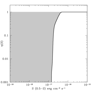
Figure 3: $Black~{}Line:$The selection function for point sources in the inner 5$\arcmin$ of the 4Ms CDFS. The $grey~{}shaded~{}area$ represents the complementary of the selection function (1-$\eta(S)$), highlighting the flux region from where the fluctuations are produced.

In Fig. 3 we show the selection function, in terms of fraction of field of view as a function of the flux limits. If $\eta(S)$ is the selection function for sources with flux S, the source counts of sources producing the shot noise is given by

$$\frac{dN_{X}}{dS}_{(SN)}=\alpha\,\left(1-\eta(S)\right)\,\frac{dN_{X}}{dS}.$$ (9)

$\alpha$ is a factor that accounts for the lower normalization observed in the CDFS with respect to larger area fields and with the Gilli et al. (2007) model (Cappelluti et al., 2009). We measured $\alpha$ by comparing the Lehmer et al. (2012) 0.5-2 keV logN-logS and the Gilli et al. (2007) modeled logN-logS at the break flux and obtained $\alpha$=0.72. We fixed the level of shot noise in our data by computing the integral in Eq. 8, by assuming that the only sources accounting for the SN are AGN and Galaxies. Therefore in this case we adopt:

$$\frac{dN_{X}}{dS}_{SN}=\frac{dN_{X}}{dS}_{AGN}+\frac{dN_{X}}{dS}_{Gal}.$$ (10)

dN/dS_AGN has been estimated from the population synthesis model of Gilli et al. (2007) and dN/dS_Gal has been computed with the model of X-ray Galaxy evolution described in Sect. 5.4. In our calculations fluxes have been converted into count-rates by assuming an average power-law spectrum with spectral index $\Gamma$=1.7. With such an assumption count-rates are obtained by multiplying the flux by an energy conversion factor ECF= 1.66$\times$10¹¹ cm²/erg. Note that a different choice of the spectral index of $\Delta\Gamma\sim\pm{0.3}$ produces a 5% variation of the ECF. The shot noise PS is scale independent (white noise) and since the signal from cosmological sources increases with the scale, the contribution of P_2,SN to the total PS becomes more important at small angular scales.
According to these prescriptions, we obtained an estimate of P_SN=1.58$\times$10^-12 cts² s^-2 deg^-4. The shot noise, as well as the other astronomical components of the PS, are affected by instrument PSF. This effect consists in a multiplicative factor that applies to the effective PS. In order to model it we used the empirical approach proposed by Churazov et al. (2011) where the PS of each modeled component is multiplied at every frequency by factor:

$$P_{PSF}(k)=\frac{1}{[1+(k/0.12)^{2}]^{1.1}},$$ (11)

where $k$ is the angular frequency. In Fig. 6 we show our estimate of P_SN, taking into account the effects of the PSF. When compared with the data we find an excellent agreement of our estimated P_SN with the Cosmic PS at short scale (i.e. $\theta<$20$\arcsec$) and we interpret this as a confirmation of our assumptions. Note that after subtracting the P_SN from P${}_{2,tot}(k)$, the remaining signal can be completely attributed to clustered sources and therefore to the sources contributing to the unresolved extragalactic CXB. In order to evaluate the strength of our detection, we computed the probability that our data could be obtained with a random fluctuation of a null flat signal. If we subtract the SN component, at $\theta>$50$\arcsec$, we still observe a strong signal. In order to determine the significance of the remaining signal, we fitted our data, on the whole angular range, with a P$(k)$=0 model (zero power signal) to determine if our signal could be due to a statistical fluctuation of a null signal. With such a model we obtained $\chi^{2}$/d.o.f.=43.5/13, thus rejecting our assumption at $>$4$\sigma$ confidence level. Since such a signal increases with scale, we interpret this as clustered cosmic signal.

5.3 Anisotropies from AGN clustering

On the small angles sampled by our data, P_2,CXB is related to the unresolved CXB production rate d$S$/d$z$, and the evolving 3D PS of the AGN, P${}_{3,AGN}(k)$ via the Limber’s equation (Peebles, 1980). At any given redshift the PS of AGN can be related to the PS of matter by knowing their redshift dependent linear biasing factor (b(z), Kaiser, 1984). Basically we have:

$$P_{3,AGN}(k,z)=b(z)^{2}P_{3,M}(k,z),$$ (12)

where P${}_{3,M}(k,z)$, is the matter 3D PS. P${}_{3,M}(k,z)$ was estimated by using the CAMB (Lewis & Bridle, 2002) tool and including in the computation both the linear and the non-linear components of the matter PS (Smith et al., 2003). Although a large amount of work on galaxies and AGN clustering is present in the literature, here we choose to combine this cosmological tool with bias measurements and predictions because of the poor sampling of the redshift space of observations. The 2D PS can be then obtained with:

$$\begin{split}&P_{2,AGN}(k)=\int^{z}_{0}\left(\alpha\,\frac{dS}{dz}\right)^{2}_{AGN}\times\\ &\frac{P_{3,AGN}(k[2\pi\,d_{A}*(1+z)]^{-1},z)}{c~{}dt/dz~{}[d_{A}*(1+z)]^{2}}~{}\frac{dz}{1+z},\end{split}$$ (13)

where d_A is the angular diameter distance, and the integration is performed in the redshift range 0$<z<$7.5. A critical point of the analysis is the determination of the flux produced by undetected AGN at any given redshift. We derived $\frac{dS}{dz}$ by using the CXB synthesis model published by Gilli et al. (2007). Briefly, the models take into account the observed luminosity function, $k$-corrections, absorption distribution and spectral shapes (see Gilli et al., 2007, for more details) of AGN and returns the observed flux at any given redshift by using:

$$\frac{dS}{dz}=\int^{\infty}_{0}\,\left(1-\eta(S)\right)\int^{z+dz}_{z}\frac{L^{\prime}}{4\pi d_{L}^{2}}\,\phi(L^{\prime},z)\,\frac{dV}{dz}\,dL^{\prime}\,dz,$$ (14)

where d_L is the luminosity distance, L^′ is the luminosity measured in the 0.5(1+z)-2(1+z) keV range and dV/dz is the comoving volume element. The values of $\frac{dS}{dz}$ have been calculated with the interactive tool provided by Gilli et al. (2007). The population of AGN used to compute the 0.5-2 keV CXB production rate has the following properties: 42$<Log(L_{X})<$47 erg/s, 20$<$Log$(N_{H})<$26 cm^-2, and 0$<z<$7.5. In addition, we included a high-redshift decline of the AGN space density (see e.g. Brusa et al., 2009; Civano et al., 2011). They indeed modeled the evolution of AGN X-ray luminosity function (XLF) at z$>$2.7 with an exponential decay ($\phi(L,z)$=$\phi$(L,z₀)$\times$10${}^{-0.43(z-z_{0})}$ and z₀=2.7) on top of the expected extrapolation from lower redshift parametrization of Hasinger et al. (2005). In Fig. 4 we show the undetected AGN CXB production rate as function of the redshift. The bulk of their flux contributing to the unresolved CXB comes from z$\sim$1.

Another important ingredient in the computation of P${}_{2,AGN}(k)$ is the bias evolution of X-ray selected AGN.

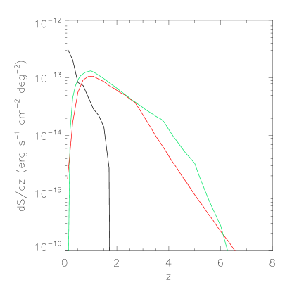
Figure 4: CXB production rate for undetected AGN ($Red~{}continuos~{}line$). Our prediction for the undetected galaxies CXB production rate is shown as $Green~{}Line$. The $black~{}line$ represents the emission from the IGM.

It has recently become clear that below z$\sim$3 AGN bias evolves like that of DM halos (DMH) of mass of $\sim$10^13.1 M_⊙ (see e.g. Cappelluti et al., 2012, for a review). However, at higher redshift the bias factor of X-ray AGN is still unknown, while for optically selected QSOs this has been modeled up to z$\sim$5 (Hopkins et al., 2007; Bonoli et al., 2009; da Ângela et al., 2008) with quadratic polynomials. In Fig. 5 we compare the prediction of Bonoli et al. (2009), rescaled to fit the z=0 X-ray selected AGN bias, and the bias computed from analytical models (van den Bosch, 2002; Sheth et al., 2001) for DMH with mass $\sim$10^13.1 M_⊙. As one can notice, both curves fit in an excellent way the observational data. Since the evolution at high-z of the AGN bias factor is unknown and still matter of debate, we assumed that the AGN bias evolves like the bias of DMH of mass $\sim$10^13.1 M_⊙ up to z$\sim$10.

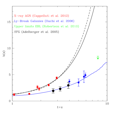
Figure 5: $Black~{}Continuous~{}Line$: Bias evolution model adopted for AGN compared with data measured by Allevato et al. (2011); ($red~{}dots$). $Black~{}dashed~{}line$: Bias evolution model for AGN of Bonoli et al. (2009). $Blue~{}line$: Bias evolution model assumed for X-ray emitting galaxies. $Black~{}pentagons:$ Bias measurements for star-forming galaxies from Adelberger et al. (2005) and with $blue~{}circles$ the measurements of bias of high-z Ly-Break galaxies of Ouchi et al. (2004). In $green$ the upper-limit from EBL fluctuations of Robertson et al. (2010)

The contribution of AGN to the overall PS is shown in Fig. 6.

5.4 Anisotropies from X-ray galaxy clustering

For anisotropies from galaxies we adopted a procedure similar to that used for AGN. The CXB production rate of galaxies has been obtained by folding in Eq. 14 the z=0 luminosity function measured by Ranalli et al. (2005) with the evolution measured for star forming galaxies by Bouwens et al. (2011). The latter provides the most recent measurement of the evolution of star formation in the Universe up to z$\sim$10 obtained with HST-WFC3. X-rays from non-active galaxies are mostly produced by low and high-mass X-ray binaries. Such objects with X-ray luminosities of $\gtrsim 10^{37}$ erg/s cannot be detected individually in distant galaxies. The contributions from fainter discrete sources (including cataclysmic variables, active binaries, young stellar objects, and supernova remnants) are well correlated with the star formation rate of the galaxy itself. However the ignition of X-ray activity in the stellar population of galaxies has a delay from the burst in star formation of the order of the time scale of stellar evolution of the donor star in binary systems. Our model does not take into account effects of the delayed switch on of X-ray Binaries from the star formation as done by e.g Ptak et al. (2001); however, our representation allowed us to model the evolution of X-ray emitting galaxies up to z=10 with the most recent results on star formation evolution.
As shown by Ranalli et al. (2005), the X-ray spectrum of galaxies can be represented by a simple power-law with spectral index $\Gamma\sim$2. With such an approximation no $k$-correction is needed.
In Fig. 4 we show the unresolved CXB production rate of galaxies as a function of the redshift. The galaxies contribution to the total flux of the unresolved CXB is dominant with respect to AGN at 0$<$z$<$6.5. Another parameter, that enters into the determination of the contribution of galaxies to the X-ray PS, is their bias factor and its evolution. Most of the modern galaxy clustering analysis papers make use of the Halo Occupation formalism and therefore it is not possible to derive an analytical formulation of the bias evolution. Moreover, galaxy clustering is complicated by the luminosity dependence of clustering (Ouchi et al., 2004). We therefore adopted a simple approximation for its determination, by assuming that the comoving correlation length of star forming galaxies is constant, in the redshift range 0$<$z$<$7.5, at the value measured by Adelberger et al. (2005) of r₀= 4.5 Mpc/h and their spatial correlation function can be modeled with a power-law with $\gamma$=1.6. Within this scenario the bias factor of galaxies can be estimated at every redshift via (Peebles, 1980):

$$b(z)=\sigma_{8,G}(z)/\sigma_{8,DM}(z),$$ (15)

where $\sigma_{8,G}$(z) is the rms fluctuations of the galaxies distribution over a sphere with radius of 8 Mpc/h and $\sigma_{8,DM}$(z) is the same quantity for DM normalized to $\sigma_{8,DM}$(z=0)=0.83. For such a power-law formalism it is possible to demonstrate that

$$(\sigma_{8,G})^{2}=J_{2}(\gamma)\left(\frac{r_{0}}{8Mpc/h}\right)^{\gamma},$$ (16)

where J₂=72/[(3-$\gamma$)(4-$\gamma$)(6-$\gamma$)2^γ] (Peebles, 1980). In Fig. 5 we compare our predicted bias evolution with the measurement of high-z Lyman break galaxies of Ouchi et al. (2004) and with upper limits derived by Robertson et al. (2010). As expected, galaxies are much less biased than AGN.

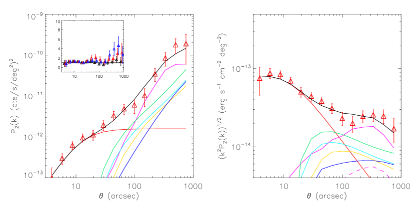
Figure 6: Left Panel. $Red~{}Triangles:$ Cosmic PS in the CDFS as a function of the scale. $Red~{}continuous~{}line:$ PS of the shot noise (Galaxies and AGN). $Green~{}continuous~{}line:$ PS of undetected AGN clustering. $Cyan~{}line$: PS of undetected galaxies clustering. $Magenta~{}continuous~{}line:$ Total power from undetected hot gas in the IGM. $Blue-line:$ predicted clustering from of mini-quasars. The $black~{}line$ represent to overall model described in Eq. 5. The inset shows the data/model ratio as a function of the scale for a SN and AGN+Galaxy clustering model ($Blue$), SN+IGM clustering model ($Red$) and SN+ AGN, Galaxies and IGM clustering model ($black$). $Right~{}Panel$: Amplitude of the fluctuations as a function of the angular scale with the same color coding as in the left panel with the addition of the contribution of IGM with 10${}^{5}<T<$10⁷ K and overdensity $\delta<$1000 following the classical definition of WHIM $Magenta~{}dashed~{}line$ to enhance its contribution to the total IGM flux. $Yellow~{}line:$ Cross-correlation contribution.

5.5 Emission from Cosmological structures and WHIM

In the inset of Fig. 6 we show that, after including the contribution of the components mentioned above, the power spectrum still shows a prominent excess signal which, although with large error bars, increases up to a factor$\sim$3-4 toward low frequencies. Another significant contribution to the total signal of the CXB may arise from emission and clustering of unresolved galaxy clusters, groups and filaments. From the sensitivity maps of galaxy clusters we determined the flux limits for galaxy cluster/group detection and converted into a luminosity limit at every redshift. For galaxy clusters and groups luminosity , mass and temperature are related by scaling relations. The relation adopted here are discussed in Finoguenov et al. (2007). The luminosity limit can be then translated into a mass limit at every redshift. Thus our source detection ensures the removal of galaxy clusters and groups down to a Log(M)=12.5-13.5 M_⊙ (i.e. kT$<$1.5 keV). Thus only the low luminosity (low mass) and warm population of galaxy groups contributes to the unresolved CXB.

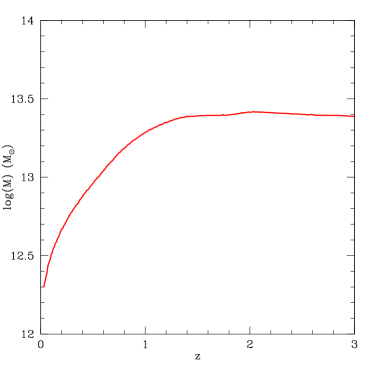
Figure 7: The $Red~{}line$ represents the lowest detectable mass in the 4Ms CDFS as a function of redshift obtained through scaling relations.

Since this class of objects is very difficult to model analytically, we describe their properties using a set of mock maps from Roncarelli et al. (2012), who used a cosmological hydrodynamical simulation to define the expected X-ray surface brightness due to the large scale structures (LSS). The original hydrodynamical simulation (see the details in Tornatore et al. 2010) follows the evolution of a comoving volume of 37.5$h^{-1}$ Mpc³ considering gravity, hydrodynamics, radiative cooling and a set of physical processes connected with the baryonic component, among which a chemical enrichment recipe that allows to follow the evolution of 7 different metal species of the intergalactic medium (IGM). From its outputs, Roncarelli et al. (2012) simulated 20 lightcones, covering the redshift interval $0<z<1.5$ with a size of $\sim$0.25 deg² (roughly 4 times the size of the CDFs) each, and angular resolution of 3.5 arcsec. Each pixel of the maps contains information about the expected observed spectrum in the 0.3–2.0 keV band with an energy resolution of 50 eV. The emission coming from the IGM was computed assuming an emission from an optically thin collisionally-ionized gas (Apec in XSPEC) model and considering the abundances of the different metal species provided by the simulation. These maps/spectra have been convolved with the Chandra response in order to reproduce the effective Chandra count rates. Since our data are masked for galaxy clusters, we applied to the simulations a source masking similar to that on the real data. The unresolved CXB production rate evaluated from simulations is shown in Fig. 4. We have simulated observations with the actual depth of the CDFS starting from the count rate maps described above, folded through a flat exposure map. We have added an artificial isotropic particle and cosmic background according to the levels estimated by Hickox & Markevitch (2006, 2007). Random Poisson noise was artificially added to the image and we ran a simple sliding cell detection with a signal to noise ratio threshold of 4. We have then excluded all the regions within which the overall encircled signal from sources is above 4 sigma with respect to the background. Since galaxy clusters and groups are highly biased, in order to smooth out effects of sample variance we extracted the power spectrum from all the masked maps and averaged the results from all the realizations. Results of the PS modeling from undetected IGM is shown in Fig. 6 (magenta solid lines). A long standing debate in astrophysics is the possibility of detecting signal in emission or in absorption from the WHIM. In order to evaluate the contribution of WHIM to the overall PS signal of the unresolved CXB, we have extracted from our simulations the same lightcones but including only all those photons with a temperature 10${}^{5}<$kT$<$10⁷ K coming from regions with matter overdensity $\delta<$1000. Such a selection is compliant to the classical definition of the WHIM, even if some denser clumps might be present also inside the filamentary structures (see the discussion in Roncarelli et al. 2012). We have masked the WHIM photon maps with the same masks used for clusters, extracted the PS and averaged over the 20 realizations. The resulting modeled PS is shown in Fig. 6 (magenta dashed lines).

5.6 Cross-Correlation terms

As mentioned above, AGN, Galaxies and IGM partially share the same large scale structures. For this reason, fluctuations are boosted by their cross-correlation term. The 3-D cross-power spectrum (CPS) of the source populations $1$ and $2$ is determined by:

$$P_{3_{1,2}}(k)=b_{1}^{2}\,b_{2}^{2}\,P_{3,M}(k,z),$$ (17)

where b₁ and b₂ are the bias factors relative to the source class 1 and 2, respectively. In analogy with the PS, the angular CPS of diffuse emission produced by two populations with background production rate $\frac{dS}{dz}_{1}$ and $\frac{dS}{dz}_{2}$, respectively, can be evaluated with the following form of the Limber’s equation:

$$\begin{split}&P_{2_{1,2}}(k)=\int^{z}_{0}\alpha^{2}\left(\frac{dS}{dz}\right)_{1}\left(\frac{dS}{dz}\right)_{2}\\ &\frac{P_{3_{1,2}}(k[2\pi\,d_{A}*(1+z)]^{-1},z)}{c~{}dt/dz~{}[d_{A}*(1+z)]^{2}}~{}\frac{dz}{1+z}.\end{split}$$ (18)

We have then computed P${}_{2_{AGN,IGM}}$, P${}_{2_{AGN,Gal}}$ and P${}_{2_{Gal,IGM}}$ using the values of bias and emissivity described above. As far as IGM is concerned we adopted the bias evolution derived from simulations where b${}_{IGM}(z)=\sqrt{1+z}$. The overall cross-power term can be then expressed as:

$$P_{2,A,G,I,}=P_{2_{AGN,IGM}}+P_{2_{AGN,Gal}}+P_{2_{Gal,IGM}}.$$ (19)

The cross power term is plotted in yellow in Fig. 6.

5.7 Accuracy of the PS model

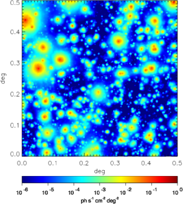
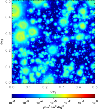
Figure 8: $Left~{}Panel:$ The whole simulation of the X-ray flux from Cosmological structure. $Right$: The same but for IGM with 10${}^{5}<$T$<$10⁷ K and overdensity $\delta<$1000.

Our CXB PS model is shown in Fig. 6 where it is compared with data. Here we summarize the ingredients adopted to model the PS components and their limits.

• At small separations most of the signal is due to shot noise produced by AGN and galaxies within the Chandra beam (red continuous line).

• The AGN clustering is modeled by convolving the matter PS for a concordance $\Lambda$-CDM cosmology, the AGN CXB production rate (dS/dz) derived from their X-ray luminosity function, and a linear bias evolution of DMH of mass Log(M)=13.1 M_⊙. Such a component increases with the scale and its rms-fluctuations (right panel) peak on scales of the order of 40-50$\arcsec$. Sources of uncertainties for such a component can be introduced by a) our assumption on the bias evolution that is unknown at z$>$2.5, b) the evolution of their luminosity function has been determined at high-z only for most luminous sources and c) the assumption at the basis of the Gilli et al. (2007) population synthesis model. Fiore et al. (2012) suggest that low-luminosity AGN may show a milder evolution at high-z with respect to observations at high luminosity. This may result in an underestimation of the power at large scale. However, as discussed above, the peak of the undetected CXB flux is produced by AGN at z$\sim$1.5, where current observations are broadly consistent.

• X-ray galaxies clustering (cyan line) is modeled by convolving the matter PS for a concordance $\Lambda$-CDM cosmology, a model of the X-ray luminosity function obtained by assuming an evolution similar to that of star forming galaxies starting from a measured z=0 XLF and a linear bias evolution of sources having a correlation length r₀=4.5 Mpc/h. As for the AGN, such a component increases with scale and its rms-fluctuations peak (right panel) on scales of the order of 50$\arcsec$. The sources of uncertainties introduced by our models are, like in the case of AGN, twofold and basically driven by our choice of the bias and XLF evolution. In the X-ray band the XLF of galaxies is known only up to z$\sim$1.5 where it follows the evolution of star formation. The limit of our approach is on the adopted model describing their cosmological evolution, which is however based on the reasonable assumption that X-ray galaxies trace star formation in the Universe. The same argument applies to bias, where no measurements have been performed in the X-ray band. However, also in this case, observational proxies are consistent with our assumptions at the redshift where the bulk of the emission is produced, and therefore limiting the margin of uncertainty of our modeling. Moreover, as we describe below, our modeling of the shot noise of AGN and galaxies is in good agreement with the data, meaning that our estimated source counts below the flux limit is statistically robust.

• The diffuse gas contribution (Magenta continuous line) is modeled by computing the PS of maps obtained by hydrodynamical cosmological simulations which include a specific recipe of chemical enrichment. Sources detectable in real observations have been excised from these simulations before computing the PS. Such a component is responsible for most of the large scale fluctuations that peak on a few arcminutes scale. For comparison, we also evaluated the expected contribution of WHIM (magenta dashed line) to the overall fluctuations and found that, on the largest angular scales, it contributes for up to $\sim$1/3 of the total power. The main source of uncertainty for this component is definitely made by the actual metallicity of the IGM in the lowest density phase which has poor observational constrains. In addition, the largest scale clustering in the simulations may be underestimated because of the limited volume sampled in our cones.

In order to test our statistical hypothesis, we performed a $\chi^{2}$ test and evaluated the improvement of the fit by adding one component after the other. We considered every component (which have their amplitude and shape fixed by our assumptions) as if they were a parameter of the fit for the evaluation of the degrees of freedom. The first test has been performed to evaluate if the observed fluctuations could be explained by the shot noise component only. As discussed above, such an hypothesis is rejected at $>$4$\sigma$ confidence level. Then we tested if, together with a shot-noise component, clustering of AGN and galaxies (including their cross power) improved the fit. In this way we obtained $\chi^{2}$/d.o.f.=17.5/12. We also performed an F-test to evaluate the probability that the obtained $\chi^{2}$ could be obtained by a statistical fluctuation of the SN only model and obtained P(F-test)=1.2$\times$10^-3, thus the inclusion of such a component significantly improves the fit. However, the relatively high $\chi^{2}$/d.o.f. value suggests that additional or different components are required.
A visual inspection suggests that the strongest feature in the PS is produced by the IGM feature. Thus we fitted the data with SN+IGM model and obtained $\chi^{2}$/d.o.f.=18.3/12 corresponding to P(F-test)=1.6$\times$10^-3 with respect to the SN only model. For such a model we show the data/model ratio in red in the inset of Fig. 6.
By adding the point source clustering (and all the cross power terms) to the latter model we obtain $\chi^{2}$/d.o.f.=7.8/11 and therefore the F-test, computed to the SN+IGM model provides P(F-test)=2.7$\times$10^-3, thus providing a further $\sim$3$\sigma$ improvement of the fit. If we compare this fit with the SN only model the F-test probility is P(F-test)=7.9$\times$10^-5, thus providing a significant improvement of the overall fit quality. The overall data/model ratio is shown in black in the inset of Fig. 6.

Model	$\chi^{2}$/d.o.f	. P(F-test)
	(1)	(2)
PSN	43.4/13
PSN+PGal+PAGN	17.5/12	1.2$\times$10-3
PSN+PIGM	18.3/12	1.6$\times$10-3
PSN+PGal+PAGN+PIGM	7.8/11	2.7$\times$10-3 *
PSN+PGal+PAGN+PIGM+Pmq	8.3/10	*

Table 1: (1) The $\chi^{2}$/d.o.f. value for model with different components include and (2), the null hypothesis probabilty obtained by adding an additional component with respect to the model with n-1 d.o.f. *:P(F-test)=7.9$\times$10^-5 with respect to the SN only model.

According to the values reported in the table, we can safely confirm that the unresolved CXB in the CDFS can be explained with random and clustered signal from undetected point sources (AGN and galaxies), IGM clustering components plus a cross correlation term.

6 Fluctuations from early black holes?

Potential contribution to the unresolved CXB and its structure can also come from very high redshifts overlapping with epochs usually identified with first stars era. It is widely expected that fragmentation within the first collapsing protogalaxies was much less efficient so that first stars were significantly more massive and short-lived and could have left behind non-negligible abundance of accreting black holes. Since, in addition, the first black holes could have also formed directly during the first stars era, these populations may supply an additional, and potentially measurable, contribution to the unresolved CXB and its fluctuations.

Spitzer-based studies have revealed significant levels of source-subtracted cosmic infrared background (CIB) fluctuations which were proposed to originate in the first stars era (Kashlinsky et al., 2005). Indeed the remaining known galaxy populations have been shown to produce significantly lower levels of the CIB fluctuations (Helgason et al., 2012) and there is no correlation in the large-scale structures between the Spitzer CIB maps at 3.6 and 4.5 micron and HST/ACS likely pointing to the high-$z$ origin of the excess CIB (Kashlinsky et al., 2007). The excess fluctuations have been confirmed in the AKARI based analysis extending to 2.4 micron (Matsumoto et al., 2011) and the signal has now been measured to extend to $\sim 1^{\circ}$ exceeding the power over the remaining normal galaxies by well over an order of magnitude (Kashlinsky, 2005). The level of the fluctuations at 3.6 micron is $\delta F_{\rm CIB}\sim 0.07$ nW/m²/sr and their energy spectrum appears to follow the Rayleigh-Jeans law, $\delta F_{\rm CIB}\propto\lambda^{-3}$, between 2.4 and 4.5 micron. If the excess CIB fluctuation arises at high $z$, the sources producing it would have projected angular density of $\sim(1-3)$arcsec^-2 (Kashlinsky et al 2007). Under the assumption that the high-z sources measured by Kashlinsky et al. (2012) rapidly evolve into miniquasars ( or early black holes), we estimated that, if the CIB/CXB flux ratio is constant along the cosmic time, with 3.6 $\mu$m extragalactic CIB flux of $\sim$6 nW m^-2 sr^-1 (Kashlinsky, 2005) and extragalactic CXB flux of 8.15$\times$10^-12 erg cm^-2 s^-1 deg^-2 (Lehmer et al., 2012), we obtain $\frac{S_{CIB}}{S_{CXB}}\sim$220. Thus we evaluated the contribution to the CXB of the CIB fluctuations to be of the order $\sim$3$\times$10^-13/(1+z) erg cm^-2 s^-1 deg^-2 (i.e. $\sim$0.5% of the CXB if these sources have z$\sim$7.5-15). We have therefore predicted the expected PS of these sources by folding their CXB production rate in Eq. 13 and integrating in the redshift range 7.5-15.
The result of this prediction is shown with a blue line in Fig. 6. A $\chi^{2}$ fit of our 5 components model provides $\chi^{2}$/d.o.f=8.3/10. Although the inclusion of such a component does not improve the quality of the fit, the statistics does not allow us to reject the hypothesis that these sources contribute to the observed fluctuations. These sources would contribute very weakly to the shot noise, and the upper limit of their contribution is not larger than the uncertainty on the measured PS. Thus at 1$\sigma$ we have P${}_{SN,mq}\lesssim$1$\times$10^-13cts² s^-2 deg^-4(i.e. the mean value of the uncertainty on those scales). According to Eq.8, we can estimate the source density of putative miniquasars with P_SN/S${}_{min}^{2}\sim$N($>S_{min}$). If S_min=10^-20erg cm^-2 s^-1 , where most CXB models predict the saturation of the source counts, we estimate N$\lesssim$60.000 deg^-2. If these sources shine in the redshift range 7.5-15 (Kashlinsky et al., 2012), then their comoving volume density is $\leq$9$\times$10^-5 Mpc^-3. For comparison in the same redshift range the Gilli et al. (2007) model predicts, for X-ray selected AGN, in the luminosity range sampled by our fluctuations (Log(L_X)$\lesssim$43.58 erg/s, at z=7.5-15, for sources with observed -20$\leq$LogS(0.5-2)$\leq$-17 erg cm^-2 s^-1), source densities of the order 1.5$\times$10^-4 Mpc^-3 and 8.4$\times$10^-5 Mpc^-3 in the case of flat and declining evolution, respectively. The upper limit derived above suggests that the declining evolution of AGN is a good representation of the evolutionary track of these remote sources.

7 Contribution of undetected source populations to the CXB

By interpreting the observed behavior of the unresolved CXB fluctuations, we have developed a model which is able to explain the nature of the unresolved CXB. The fluctuations observed here are reproduced in the PS if the clustering recipes described in the text are combined with the unresolved CXB production rates shown in Table 2.

Table 2: (1) CXB production rate of every class of undetected sources. (2) The percentage of the overall and (3) unresolved CXB produced by every population. In the last line we show the cumulative values, the ranges refer to Model I and II.

Component	S	% CXBa	% Unres. CXB
	$\times$10-13erg cm-2 s-1 deg-2	%	%
	(1)	(2)	(3)
AGN	1.97	2.4$\pm{0.2}$	19.3$\pm{1.3}$
Galaxies	2.51	3.1$\pm{0.2}$	24.6$\pm{1.7}$
IGM	5.70	7.0$\pm{0.5}$	55.9$\pm{3.9}$
bWHIM	1.70	2.1$\pm{0.1}$	16.7$\pm{1.2}$
Early-BH	$<$0.35	$<$0.5	$<$3.4
Total	10.18	12.4$\pm{0.9}$	100

^a: Computed using a total 0.5-2 keV CXB flux of 8.15$\pm{0.58}\times$10^-12erg cm^-2 s^-1 deg^-2 (Lehmer et al., 2012).
^b:The WHIM flux is included in the IGM flux.

Our results show that, in the 0.5-2 keV band, the effective fraction of the unresolved extragalactic background is of the order of 12% of the total. In Table 2 we show the CXB flux that our model predicts to explain the fluctuations together with the fractions of total and unresolved CXB produced by every undetected source population. As one can notice in Table 2, the bulk ($\sim$56%) of the unresolved CXB flux is made by unresolved clusters, groups and the WHIM which accounts, by itself, for $\sim$17% of the unresolved flux.
For point sources our model predicts that AGN and galaxies contribute, all together, for the remaining flux of the unresolved CXB, with galaxies and AGN producing $\sim$25% and $\sim$20% of the unresolved flux, respectively.
Moreover, our data cannot exclude that a sizeable fraction of the unresolved CXB could be produced by a population of still undetected high-z sources, likely black hole seeds.

8 Discussion

In this paper we presented the measurement of the angular PS of the fluctuations of the unresolved CXB in the 4Ms observation of the CDFS in the angular range $\lesssim 10\arcmin$. Poisson noise and spurious signals have been modeled and removed from the measured PS. We performed a spectral decomposition analysis and showed that after removing the low frequency signal, which can be attributed to the shot noise of unresolved sources that randomly enter the beam, the amplitude of the fluctuations with extragalactic origin account for $\sim$12.3% of the CXB and the significance of the detection of these cosmic fluctuations is $>$10$\sigma$. In the next section we briefly discuss to properties of the populations producing the unresolved CXB fluctuations.

8.1 The population of undetected AGN

For AGN we folded the observed evolution scenarios with the population synthesis model of Gilli et al. (2007) and a simple recipe for bias where AGN are tracing DMH with mass Log(M)=13.1 M_⊙.

This population of AGN has a space density that exponentially declines above z=2.7. The CXB production rate necessary to produce the modeled PS yields to a fraction of the unresolved 0.5-2 keV CXB flux of $\sim$19%. We predicted a CXB flux produced by undetected AGN of $\sim$2.0$\times$10^-13 erg cm^-2 s^-1 deg^-2.

We also tried to probe different evolution scenarios but our data do not allow to significantly constrain the behavior of the AGN XLF at high-z. In Fig. 9 we show the predicted LogN-LogS that, according to our model, satisfies the observed fluctuations compared with recent observations.

8.2 The population of undetected X-ray galaxies

Galaxies are the most numerous population of objects contributing to the unresolved CXB (see Fig. 9); the power produced by such a population is lower that that of AGN since they are less biased even if they produce more CXB flux. In the soft X-rays, galaxies have been observed up to z$\sim$1 (see e.g. Lehmer et al., 2007), and therefore their high-z space density is unknown. We have developed a toy model for the galaxies XLF where their evolution follows that of the star formation in the universe. With this model we estimated that galaxies contribute to $\sim$25% of the unresolved CXB flux. In a recent paper, Dijkstra et al. (2012) used a modeling similar to ours and found that, in principle, X-ray galaxies could produce all of the unresolved 1-2 keV CXB. However they did not consider the contribution of other undetected sources that we have shown to produce a large fraction of the unresolved CXB. Overall, the predicted source counts of AGN and galaxies are in good agreement with the measurements of Xue et al. (2011) and Lehmer et al. (2012) in the same field.

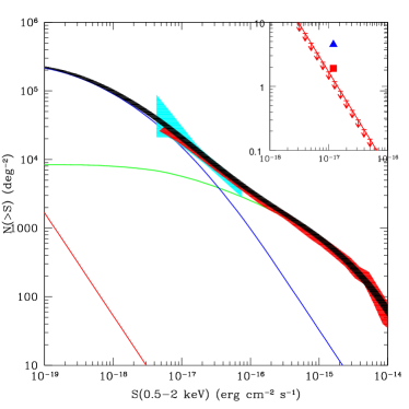
Figure 9: The 0.5-2 keV logN-logS used to reproduce the observed unresolved CXB fluctuations. In $green$ AGN, $blue$ galaxies and, in $black-shaded$, the sum of the AGN and galaxies, the uncertainty is attributed to the count-rate to flux conversion. The $red~{}shaded~{}area$ is the logN-logS measured by Lehmer et al. (2012) in the CDFS. The $red~{}line$ represents the upper limit of the logN-logS of miniquasars. The $cyan~{}shaded~{}area$ represents the expected counts from the fluctuation analysis of Miyaji & Griffiths (2002). In the inset we show a zoom onto the miniquasar upper-limit logN-logS. The $blue~{}triangle$ is the expected number of X-ray sources, at the flux limit of the 4Ms CDFS, produced at z$\lesssim$10 from collapse of POPIII stars accreting at the Eddington Limit. The $red~{}triangle$ is number of X-ray sources in case of of direct collapse (Quasi-stars) accreting at $\lambda_{Edd}$=0.3

8.3 CXB from IGM and WHIM

On scales larger than 100$\arcsec$ our analysis shows that the main contribution to the unresolved CXB fluctuations is due to IGM emission produced by undetected groups, clusters and the WHIM. This has been estimated with cosmological hydrodynamical simulations that, together with structure formation, include feedback mechanisms that pollute the IGM with metals which are responsible for the X-ray emission (Roncarelli et al., 2012). Such a component produces $\sim$50% of the unresolved CXB.
We determined that $\sim$1/3 of the IGM flux is produced by the WHIM, where the so called ”missing baryons” are expected to lie. However the WHIM definition taken from simulations already applies a density cut ($\delta<1000$) that is meant to mimic roughly the effect of excising detected sources. In reality, dense clumps may be present outside virialized objects so we must consider our determination as a lower limit of the total WHIM contribution (see the discussions in Roncarelli et al. 2006, 2012).

Our model thus predicts that the flux of the WHIM in the CDFS is of the order 1.7$\times$10^-13 erg cm^-2 s^-1 deg^-2 (i.e. 2.3% of the total CXB flux) and produces a signal peaking on a few arcmin scale. Such an estimate is about one order of magnitude lower than what measured by Galeazzi et al. (2009) (i.e. 12% of the overall diffuse emission in shallower 0.2-0.4 keV XMM-Newton observations) where they did not model the contamination from undetected sources. However such an estimate relies on the output of the simulation and is very sensitive to the metallicity of the WHIM. According to Roncarelli et al. (2012), different recipes for the metal enrichment of the WHIM may lead to a variation up to a factor 3 in overall emissivity of the WHIM. More information on such a component of the Universe will be possible if, for example, contamination of undetected cluster could be excised from X-ray maps by masking also optically detected groups with mass Log(M)$>$12-12.5 M_⊙.

8.4 Very high-z sources

Finally, we speculated on the possible existence of a population of high-z miniquasars (or early black holes) born from the collapse of early massive objects. Although we did not detect their signature, we placed an upper limit to their contribution to the CXB ($<$3$\times$10^-13/(1+z) erg cm^-2 s^-1 deg^-2, z$>$7.5). We estimated that these sources would follow the declining evolutionary track of AGN with Log(L_X)$\lesssim$43.58 erg/s.
Our observations are not sensitive to the faint fluxes expected from these sources, and thus we could only place upper limits. However, since such a population peaks at z$>7.5$, their fluctuations should peak on scales of the order of several tens of arcminutes, where the contribution from shot-noise is relatively weak also in shallower surveys. On such a scale, foreground source population PS significantly dims and therefore their detection would be possible. To conclude, we determined that at fluxes of the order 10^-20 erg cm^-2 s^-1, their number density is order of $\sim$60000 deg^-2 which means that, under the assumption of Euclidean logN-logS, at the flux limit of the CDFS their number density is of the order 1-2 deg^-2.
Using the theoretical predictions of Volonteri (2010), Treister et al. (2011) computed the expected number density of the first X-ray sources at z$\sim$7-10 at the 4Ms CDFS flux limit. In the case of Population III stars remnants accreting at the Eddington limit they find 4.5 deg^-2, while in the case of direct collapse (quasi-stars, Begelman et al., 2008) with accretion regime at $\lambda_{Edd}$=0.3 their expected number density is 1.9 deg^-2. In Fig. 9 we show a comparison of these predictions with our upper-limit which, at the zero-th order, is favoring the direct collapse scenario.

Our work suggests that future deeper observations on wider fields would allow us to improve the sensitivity of the PS measurement by reducing the Shot-Noise and masking fainter clusters. Moreover a deep survey with a flux limit comparable or deeper to that of the 4Ms CDFS covering 1-2 deg², would allow us a direct detection of the WHIM feature and, by measuring the large scale shape of the PS, investigate the very high-z X-ray Universe. A possible future X-ray mission like the proposed Wide Field X-ray Telescope (WFXT Giacconi et al., 2009) will be able to study the PS of the unresolved CXB with high precision given the large collecting area (low photon noise) and the large field of view (low cosmic variance).

References

- Adelberger et al. (2005) Adelberger, K. L., Steidel, C. C., Pettini, M., et al. 2005, ApJ, 619, 697
- Allevato et al. (2011) Allevato, V., Finoguenov, A., Cappelluti, N., et al. 2011, ApJ, 736, 99
- Arevalo et al. (2012) Arevalo, P., Churazov, E., Zhuravleva, I., Hernandez-Monteagudo, C., & Revnivtsev, M. 2012, arXiv:1207.5825
- Barcons et al. (1998) Barcons, X., Fabian, A. C., & Carrera, F. J. 1998, MNRAS, 293, 60
- Bauer et al. (2004) Bauer, F. E., Alexander, D. M., Brandt, W. N., et al. 2004, AJ, 128, 2048
- Begelman et al. (2008) Begelman, M. C., Rossi, E. M., & Armitage, P. J. 2008, MNRAS, 387, 1649
- Bonoli et al. (2009) Bonoli, S., Marulli, F., Springel, V., et al. 2009, MNRAS, 396, 423
- Brandt et al. (2001) Brandt, W. N., Alexander, D. M., Hornschemeier, A. E., et al. 2001, AJ, 122, 2810
- Brunner et al. (2008) Brunner, H., Cappelluti, N., Hasinger, G., et al. 2008, A&A, 479, 283
- Brusa et al. (2009) Brusa, M., Comastri, A., Gilli, R., et al. 2009, ApJ, 693, 8
- Cappelluti et al. (2009) Cappelluti, N., Brusa, M., Hasinger, G., et al. 2009, A&A, 497, 635
- Cappelluti et al. (2012) Cappelluti, N., Allevato, V., & Finoguenov, A. 2012, Advances in Astronomy, 2012,
- Cen & Ostriker (1999) Cen, R., & Ostriker, J. P. 1999, ApJ, 514, 1
- Cen & Fang (2006) Cen, R., & Fang, T. 2006, ApJ, 650, 573
- Civano et al. (2011) Civano, F., Brusa, M., Comastri, A., et al. 2011, ApJ, 741, 91
- Churazov et al. (2011) Churazov, E., Vikhlinin, A., Zhuravleva, I., et al. 2011, arXiv:1110.5875
- da Ângela et al. (2008) da Ângela, J., Shanks, T., Croom, S. M., et al. 2008, MNRAS, 383, 565
- Diego et al. (2003) Diego, J. M., Sliwa, W., Silk, J., & Barcons, X. 2003, MNRAS, 344, 951
- Dijkstra et al. (2012) Dijkstra, M., Gilfanov, M., Loeb, A., & Sunyaev, R. 2012, MNRAS, 421, 213
- Eckmiller et al. (2011) Eckmiller, H. J., Hudson, D. S., & Reiprich, T. H. 2011, A&A, 535, A105
- Fabian & Barcons (1992) Fabian, A. C., & Barcons, X. 1992, ARA&A, 30, 429
- Fang et al. (2010) Fang, T., Buote, D. A., Humphrey, P. J., et al. 2010, ApJ, 714, 1715
- Finoguenov et al. (2007) Finoguenov, A., Guzzo, L., Hasinger, G., et al. 2007, ApJS, 172, 182
- Fiore et al. (2012) Fiore, F., Puccetti, S., Grazian, A., et al. 2012, A&A, 537, A16
- Fukugita et al. (1998) Fukugita, M., Hogan, C. J., & Peebles, P. J. E. 1998, ApJ, 503, 518
- Galeazzi et al. (2009) Galeazzi, M., Gupta, A., & Ursino, E. 2009, ApJ, 695, 1127
- Gilli et al. (2007) Gilli, R., Comastri, A., & Hasinger, G. 2007, A&A, 463, 79
- Giacconi et al. (2001) Giacconi, R., Rosati, P., Tozzi, P., et al. 2001, ApJ, 551, 624
- Giacconi et al. (2009) Giacconi, R., Borgani, S., Rosati, P., et al. 2009, astro2010: The Astronomy and Astrophysics Decadal Survey, 2010, 90
- Gilli et al. (1999) Gilli, R., Risaliti, G., & Salvati, M. 1999, A&A, 347, 424
- Hasinger et al. (2005) Hasinger, G., Miyaji, T., & Schmidt, M. 2005, A&A, 441, 417
- Hopkins et al. (2007) Hopkins, P. F., Lidz, A., Hernquist, L., et al. 2007, ApJ, 662, 110
- Hickox & Markevitch (2006) Hickox, R. C., & Markevitch, M. 2006, ApJ, 645, 95
- Kaiser (1984) Kaiser, N. 1984, ApJ, 284, L9
- Kashlinsky et al. (1996) Kashlinsky, A., Mather, J. C., Odenwald, S., & Hauser, M. G. 1996, ApJ, 470, 681
- Kashlinsky (2005) Kashlinsky, A. 2005, Phys. Rep., 409, 361
- Kashlinsky et al. (2005) Kashlinsky, A., Arendt, R. G., Mather, J., & Moseley, S. H. 2005, Nature, 438, 45
- Kashlinsky et al. (2007) Kashlinsky, A., Arendt, R. G., Mather, J., & Moseley, S. H. 2007, ApJ, 654, L5
- Kashlinsky et al. (2012) Kashlinsky, A., Arendt, R. G., Ashby, M. L. N., et al. 2012, arXiv:1201.5617
- Kaastra et al. (2006) Kaastra, J. S., Werner, N., Herder, J. W. A. d., et al. 2006, ApJ, 652, 189
- Helgason et al. (2012) Helgason, K., Ricotti, M., & Kashlinsky, A. 2012, ApJ, 752, 113
- Hickox & Markevitch (2006) Hickox, R. C., & Markevitch, M. 2006, ApJ, 645, 95
- Hickox & Markevitch (2007) Hickox, R. C., & Markevitch, M. 2007, ApJ, 661, L117
- Lehmer et al. (2007) Lehmer, B. D., Brandt, W. N., Alexander, D. M., et al. 2007, ApJ, 657, 681
- Lehmer et al. (2012) Lehmer, B. D., Xue, Y. Q., Brandt, W. N., et al. 2012, arXiv:1204.1977
- Lemze et al. (2009) Lemze, D., Sadeh, S., & Rephaeli, Y. 2009, MNRAS, 397, 1876
- Lewis & Bridle (2002) Lewis, A., & Bridle, S. 2002, Phys. Rev. D, 66, 103511
- Luo et al. (2008) Luo, B., et al. 2008, ApJS, 179, 19
- Luo et al. (2011) Luo, B., Brandt, W. N., Xue, Y. Q., et al. 2011, ApJ, 740, 37
- Madau et al. (2004) Madau, P., Rees, M. J., Volonteri, M., Haardt, F., & Oh, S. P. 2004, ApJ, 604, 484
- Martin-Mirones et al. (1991) Martin-Mirones, J. M., de Zotti, G., Franceschini, A., et al. 1991, ApJ, 379, 507
- Matsumoto et al. (2011) Matsumoto, T., Seo, H. J., Jeong, W.-S., et al. 2011, ApJ, 742, 124
- Miyaji & Griffiths (2002) Miyaji, T., & Griffiths, R. E. 2002, ApJ, 564, L5
- Moretti et al. (2003) Moretti, A., Campana, S., Lazzati, D., & Tagliaferri, G. 2003, ApJ, 588, 696
- Nicastro et al. (2005) Nicastro, F., Mathur, S., Elvis, M., et al. 2005, Nature, 433, 495
- Ouchi et al. (2004) Ouchi, M., Shimasaku, K., Okamura, S., et al. 2004, ApJ, 611, 685
- Peebles (1980) Peebles P. J. E., 1980, The Large Scale Structure of the Universe (Princeton: Princeton Univ. Press)
- Ptak et al. (2001) Ptak, A., Griffiths, R., White, N., & Ghosh, P. 2001, ApJ, 559, L91
- Ranalli et al. (2005) Ranalli, P., Comastri, A., & Setti, G. 2005, A&A, 440, 23
- Roncarelli et al. (2006) Roncarelli, M., Moscardini, L., Tozzi, P., et al. 2006, MNRAS, 368, 74
- Ranalli et al. (2012) Ranalli, P., et al. 2012, in preparation
- Roncarelli et al. (2012) Roncarelli, M., Cappelluti, N., Borgani, S., Branchini, E., & Moscardini, L. 2012, MNRAS, 3218
- Robertson (2010) Robertson, B. E. 2010, ApJ, 716, L229
- Schneider et al. (2002) Schneider, R., Ferrara, A., Natarajan, P., & Omukai, K. 2002, ApJ, 571, 30
- Shull et al. (2011) Shull, J. M., Smith, B. D., & Danforth, C. W. 2011, arXiv:1112.2706
- Salvaterra et al. (2005) Salvaterra, R., Haardt, F., & Ferrara, A. 2005, MNRAS, 362, L50
- Setti & Woltjer (1989) Setti, G., & Woltjer, L. 1989, A&A, 224, L21
- Sheth et al. (2001) Sheth R. K., Mo H. J., Tormen G. 2001, MNRAS, 323, 1
- Śliwa et al. (2001) Śliwa, W., Soltan, A. M., & Freyberg, M. J. 2001, A&A, 380, 397
- Sołtan & Hasinger (1994) Soltan, A., & Hasinger, G. 1994, A&A, 288, 77
- Sołtan et al. (2002) Sołtan, A. M., Freyberg, M. J., & Hasinger, G. 2002, A&A, 395, 475
- Sołtan (2006) Sołtan, A. M. 2006, A&A, 460, 59
- Smith et al. (2003) Smith, R. E., Peacock, J. A., Jenkins, A., et al. 2003, MNRAS, 341, 1311
- Takei et al. (2011) Takei, Y., Ursino, E., Branchini, E., et al. 2011, ApJ, 734, 91
- Tornatore et al. (2010) Tornatore, L., Borgani, S., Viel, M., & Springel, V. 2010, MNRAS, 402, 1911
- Treister & Urry (2006) Treister, E., & Urry, C. M. 2006, ApJ, 652, L79
- Treister et al. (2011) Treister, E., Schawinski, K., Volonteri, M., Natarajan, P., & Gawiser, E. 2011, Nature, 474, 356
- Ursino & Galeazzi (2006) Ursino, E., & Galeazzi, M. 2006, ApJ, 652, 1085
- van den Bosch (2002) van den Bosch, F. C., 2002, MNRAS, 331, 98
- Xue et al. (2011) Xue, Y. Q., et al. 2011, arXiv:1105.5643
- Vecchi et al. (1999) Vecchi, A., Molendi, S., Guainazzi, M., Fiore, F., & Parmar, A. N. 1999, A&A, 349, L73
- Volonteri (2010) Volonteri, M. 2010, A&A Rev., 18, 279
- Wu & Anderson (1992) Wu, X., & Anderson, S. F. 1992, AJ, 103, 1