Synthetic Topological Degeneracy by Anyon Condensation

Abstract

Topological degeneracy is the degeneracy of the ground states in a many-body system in the large-system-size limit. Topological degeneracy cannot be lifted by any local perturbation of the Hamiltonian. The topological degeneracies on closed manifolds have been used to discover/define topological order in many-body systems, which contain excitations with fractional statistics. In this paper, we study a new type of topological degeneracy induced by condensing anyons along a line in 2D topological ordered states. Such topological degeneracy can be viewed as carried by each end of the line-defect, which is a generalization of Majorana zero-modes. The topological degeneracy can be used as a quantum memory. The ends of line-defects carry projective non-Abelian statistics, and braiding them allow us to perform fault tolerant quantum computations.

Introduction— The topological degeneracy associated to the topological defects in the topologically ordered statestopo order has attracted much research interests recentlyBarkeshliWen ; BarkeshliQi ; BarkeshliJianQi ; Clarke ; Lindner ; MCheng ; Vaezi ; Bombin ; KitaevKong ; YouWen ; Ran . Examples have been found in $K$-matrixKmat $\bigl{(}\begin{smallmatrix}N&0\\ 0&N\end{smallmatrix}\bigr{)}$ or $\bigl{(}\begin{smallmatrix}N&0\\ 0&-N\end{smallmatrix}\bigr{)}$ quantum Hall systemsBarkeshliWen ; BarkeshliQi ; BarkeshliJianQi ; Clarke ; Lindner ; MCheng ; Vaezi , and in $\mathbb{Z}_{N}$ gauge theory ($K=\bigl{(}\begin{smallmatrix}0&N\\ N&0\end{smallmatrix}\bigr{)}$)Bombin ; KitaevKong ; YouWen , where the topological defects are rendered into projective non-Abelian anyonspnAa due to the interplay between the space geometry and the topological order. In most of the cases, the topological defects are realized as lattice dislocations involving non-local deformation of the lattice structure. The difficulty of manipulating lattice dislocations hinders the physical realization of fusing or braiding these projective non-Abelian anyons. Therefore we are motivated to design flexible and movable synthetic dislocations. The same motivation also leads to the proposal of synthetic dislocations in the bilayer FQH systems by zig-zag gatinggating . In this work, we show that it is possible to mimic the lattice dislocations by applying some external field to a line of sites (along the dislocation branch-cut) without altering the underlying lattice structure. The external field quenches the degrees of freedom on those sites, as if they were removed from the lattice effectively. As the external field can be turned on and off, the synthetic dislocations can be produced and moved around physically. On the other hand, the external field (or coupling) also drives intrinsic anyon condensationKitaevKong ; anyoncond along the branch-cut line, which demonstrates the designing principle of synthetic dislocations by anyon condensation. This makes synthetic dislocations more general than the lattice dislocations, since we can choose to condense different types of anyons, which in turn generates different kinds of topological degeneracies, associated to different synthetic dislocations with different projective non-Abelian statistics.

Synthetic Dislocations— We start from the $\mathbb{Z}_{2}$ plaquette modelWen plaq (or the Kitaev toric code modelKitaev ), whose low energy effective theory is a $\mathbb{Z}_{2}$ lattice gauge theory. It has been shownYouWen that each lattice dislocation in this model is associated to a Majorana zero mode. On the other hand, the $\mathbb{Z}_{2}$ gauge theory supports (bulk) Majorana fermion excitations (denoted by $em$) as the bound state of $\mathbb{Z}_{2}$ electric and magnetic charges. If one condenses these Majorana fermions along a line segment in the lattice by lowering their excitation energy, then the Majorana zero modes will also emerge at the ends of the chain.MajChain Our conjecture is that the Majorana zero modes at the ends of a Majorana chain (a line of Majorana fermion condensate) and the Majorana zero modes associated to the extrinsic lattice dislocations are physically equivalent. If this is true, we can create synthetic dislocations by condensing the Majorana fermions.

To verify the above conjecture, consider the $\mathbb{Z}_{2}$ plaquette model on a square lattice with one qubit per site, which is described by Hamiltonian $H_{0}=-\sum_{p}O_{p}$, where $O_{p}$ is a product of operators around the plaquette $p$,

$$O_{p}=\vbox{\hbox{\includegraphics[height=24.0pt]{fig_Z2Op.pdf}}}=\sigma_{1}^{z}\sigma_{2}^{x}\sigma_{3}^{z}\sigma_{4}^{x}.$$ (1)

Here we have adopted the graphical representation as introduced in Ref. YouWen , where each operator acting on the qubit is represented by a string going through that site, i.e. $\sigma_{i}^{z}={\vbox{\hbox{\includegraphics[height=10.0pt]{fig_sz.pdf}}}}_{i}$ and $\sigma_{i}^{x}={\vbox{\hbox{\includegraphics[height=10.0pt]{fig_sx.pdf}}}}_{i}$. These operators follow the algebra $\sigma_{i}^{x}\sigma_{i}^{z}=-\sigma_{i}^{z}\sigma_{i}^{x}$, or as $\vbox{\hbox{\includegraphics[height=10.0pt]{fig_sxsz.pdf}}}=-\vbox{\hbox{\includegraphics[height=10.0pt]{fig_szsx.pdf}}}$. The ground state of this model is a condensate of closed strings (generated by $O_{p}$ operators). Intrinsic excitations are created by the open string operator at both of its ends. Excitations in the even (odd) plaquettes are called electric (magnetic), denoted by $e$ ($m$). The fermion excitation is composed of a pair of electric and magnetic excitations in the neighboring plaquettes, which can be created (in pair) by the action of $\sigma_{i}^{y}=i\,{\vbox{\hbox{\includegraphics[height=10.0pt]{fig_sy.pdf}}}}_{i}=i\sigma_{i}^{x}\sigma_{i}^{z}$ on a site, as illustrated in Fig. 1. Further acting $\sigma_{i+1}^{y}$ will move one fermion to the next double plaquette ( ). Thus the action of $\sigma_{i}^{y}$ can be translated as $\sigma_{i}^{y}=c_{q}^{\dagger}c_{q+1}^{\dagger}+c_{q}^{\dagger}c_{q+1}+h.c.$, in terms of the fermion creation $c_{q}^{\dagger}$ and annihilation $c_{q}$ operators, with $q$ labeling the double plaquette, see Fig. 1. Therefore to make a Majorana chain we only need to add $\sigma^{y}$ terms to the Hamiltonian along a line of sites (in the region $\mathcal{C}$), as $H=-\sum_{p}O_{p}+g\sum_{i\in\mathcal{C}}\sigma_{i}^{y}$. The fermions are restricted to move along the chain, because there is no operator like $\sigma^{y}$ elsewhere to take the fermions away. Each fermion excitation carries 4 units of energy according to the $O_{p}$ term in the Hamiltonian $H$, so we can write down the Hamiltonian for the fermions along the chain: $H_{\mathcal{C}}=g\sum_{q\in\mathcal{C}}(c_{q}^{\dagger}c_{q+1}^{\dagger}+c_{q}^{\dagger}c_{q+1}+h.c.)+4\sum_{q\in\mathcal{C}}c_{q}^{\dagger}c_{q}$. For small $g$, $H_{\mathcal{C}}$ is in its trivial phase. For $g$ greater than the critical value $g_{c}=2$, $H_{\mathcal{C}}$ will be driven into the weak pairing phase,weak pairing with Majorana zero modes at both ends of $\mathcal{C}$. Therefore we can condense the intrinsic fermion excitations and make a Majorana chain by applying strong “transverse” field $g$. This Majorana chain will become the branch-cut line between the synthetic dislocations.

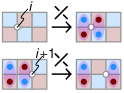
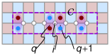
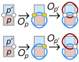
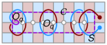
Figure 1: (Color online.) The lattice is partitioned into even and odd plaquettes, which respectively host electric $\vbox{\hbox{\includegraphics[height=8.0pt]{fig_e.pdf}}}\equiv e$ and magnetic $\vbox{\hbox{\includegraphics[height=8.0pt]{fig_m.pdf}}}\equiv m$ excitations. 1 The on-site action of $\sigma^{y}$ operator creates, annihilates or moves fermion excitations. 1 Turn on $\sigma^{y}$ term along a line of sites (marked by ) to condense the fermions into a Majorana chain. The chain (branch-cut) region $\mathcal{C}$ is outlined by the dashed line. 1 The 2nd order perturbation paths leading to the double-plaquette operators. Excited sites in the intermediate states are marked by . 1 The double-plaquette operators on the branch-cut and around the synthetic dislocation.

The strong $g$ field along the branch-cut line quenches the qubit degrees of freedom, which effectively removes those sites from the lattice, leading to the synthetic dislocations at the ends. To justify this statement, we start from $H=-\sum_{p}O_{p}+g\sum_{i\in\mathcal{C}}\sigma_{i}^{y}$ in the large $g$ limit. The qubits along the branch-cut are polarized by the $g$ field to the $\sigma^{y}_{i}=-1$ state. Any plaquette operator $O_{p}$ that crosses the branch-cut will excite the qubits at the crossing points to the $\sigma_{i}^{y}=+1$ state and thus taking the system to the high energy sector (of the energy $\sim g$), as illustrated in Fig. 1. Such a high energy state can be brought back to the low energy sector immediately either by acting the same $O_{p}$ again or by another plaquette operator $O_{p^{\prime}}$ which shares the same crossing points. Besides those, any other plaquette operators will leave the system in the high energy sector, leading to higher order perturbations. So $O_{p}\to O_{p}$ and $O_{p}\to O_{p^{\prime}}$ are the only possible paths for perturbation up to the 2nd order. However the former will only produce a constant shift in energy, which is not interesting; while the later leads to the effective Hamiltonian $H_{\text{eff}}=-\sum_{p\notin\mathcal{C}}O_{p}-1/(2g)(\sum_{q\in\mathcal{C}}O_{q}+2\sum_{q\in\partial\mathcal{C}}O_{q})$ acting in the low energy subspace where no qubit on the branch-cut line is excited. Here $q$ labels the double plaquettes across the branch-cut ($q\in\mathcal{C}$) or around the dislocations ($q\in\partial\mathcal{C}$). The double-plaquette operators $O_{q}$ are given by

$$\begin{split}O_{q\in\mathcal{C}}&=\vbox{\hbox{\includegraphics[height=24.0pt]{fig_Z2Ol.pdf}}}=\sigma_{1}^{z}\sigma_{2}^{x}\sigma_{3}^{z}\sigma_{4}^{x},\\ O_{q\in\partial\mathcal{C}}&=i\,\vbox{\hbox{\includegraphics[height=24.0pt]{fig_Z2Oe.pdf}}}=\sigma_{1}^{z}\sigma_{2}^{x}\sigma_{3}^{z}\sigma_{4}^{x}(-\sigma_{5}^{y}),\end{split}$$ (2)

whose arrangement is shown in Fig. 1. These double-plaquette operators effectively sew up the branch-cut by coupling the qubits across, and leaving the qubits right on the branch-cut untouched (as their degrees of freedom has been frozen by the $g$ field). Electric and magnetic strings are glued together in the branch-cut region by the double-plaquette operators, which is evidenced from $[S,O_{q}]=0$ (take $S$ in Fig. 1 for example) such that no excitation is left on the branch cut by the action of $S$. This explicitly demonstrate that going through the branch-cut line, $e$ charge will become $m$ and vice versa, realizing the $e$-$m$ duality, which is the defining property of dislocation branch-cut in the $\mathbb{Z}_{2}$ plaquette model.

Therefore the dislocation associated to the $e$-$m$ duality can be synthesized by condensing the fermion excitations into a Majorana chain, instead of deforming the lattice literally. The synthetic dislocations mimic all the defining physical properties of real lattice dislocations, such as implementing the $e$-$m$ duality as the intrinsic excitations winding around, and carrying the synthetic Majorana zero mode. Moreover, they are flexible and movable, as controlled by the applied field $g$, so their fusion and braiding can be discussed in a more physical sense.

Synthetic Non-Abelian Anyons— The above discussion can be readily generalized to the $\mathbb{Z}_{N}$ plaquette model,ZN1 ; ZN2 with one $\mathbb{Z}_{N}$ rotor per site, governed by the Hamiltonian $H_{0}=-\frac{1}{2}\sum_{p}O_{p}+h.c.$, where the single plaquette operator is defined as

$$O_{p}=\vbox{\hbox{\includegraphics[height=24.0pt]{fig_ZNOp.pdf}}}=U_{1}V_{2}U_{3}^{\dagger}V_{4}^{\dagger},$$ (3)

with the on-site operators $U_{i}={\vbox{\hbox{\includegraphics[height=10.0pt]{fig_U.pdf}}}}_{i}$ and $V_{i}={\vbox{\hbox{\includegraphics[height=10.0pt]{fig_V.pdf}}}}_{i}$ following the Weyl group algebra $V_{i}U_{i}=e^{i\theta_{N}}U_{i}V_{i}$ (with $\theta_{N}\equiv\frac{2\pi}{N}$), or $\vbox{\hbox{\includegraphics[height=10.0pt]{fig_VU.pdf}}}=e^{i\theta_{N}}\vbox{\hbox{\includegraphics[height=10.0pt]{fig_UV.pdf}}}$. Again, synthetic dislocations can be produced by simply modifying the Hamiltonian to $H=-\frac{1}{2}\sum_{p}O_{p}-\frac{1}{2}g\sum_{i\in\mathcal{C}}X_{i}+h.c.$, where $X_{i}=-e^{-i\theta_{N}/2}{\vbox{\hbox{\includegraphics[height=10.0pt]{fig_X.pdf}}}}_{i}=-e^{-i\theta_{N}/2}U_{i}V_{i}^{\dagger}$. Strong enough $g$ field will quench the rotor degrees of freedom by polarization to the $X_{i}=+1$ state, which effectively removes the sites along the branch-cut $\mathcal{C}$. In the large $g$ limit, the low energy effective Hamiltonian follows from the 2nd order perturbation: $H_{\text{eff}}=-\frac{1}{2}\sum_{p\notin\mathcal{C}}O_{p}-1/(4g\sin^{2}\frac{\theta_{N}}{2})(\sum_{q\in\mathcal{C}}O_{q}+2\sum_{q\in\partial\mathcal{C}}O_{q})+h.c.$, with the double-plaquette operators given by

$$\begin{split}O_{q\in\mathcal{C}}&=\vbox{\hbox{\includegraphics[height=24.0pt]{fig_ZNOl.pdf}}}=U_{1}V_{2}U_{3}^{\dagger}V_{4}^{\dagger},\\ O_{q\in\partial\mathcal{C}}&=-e^{-i\frac{\theta_{N}}{2}}\,\vbox{\hbox{\includegraphics[height=24.0pt]{fig_ZNOe.pdf}}}=U_{1}V_{2}U_{3}^{\dagger}V_{4}^{\dagger}X_{5}.\end{split}$$ (4)

The double-plaquette operators glue the $\mathbb{Z}_{N}$ electric and magnetic strings together, realizing the $e$-$m$ duality across the branch-cut. Synthetic dislocations are created at both ends. It has been shownYouWen that each of these dislocations resembles a projective non-Abelian anyon of quantum dimension $\sqrt{N}$.supplementary

The point of introducing dislocations is to produce the non-Abelian anyons. In the $\mathbb{Z}_{2}$ plaquette model, Majorana zero modes were produced by condensing the fermions $em$ along a line. Now the same idea is generalized to the $\mathbb{Z}_{N}$ plaquette model. From the graphical representation $X_{i}=-e^{-i\theta_{N}/2}{\vbox{\hbox{\includegraphics[height=10.0pt]{fig_X.pdf}}}}_{i}$, it is clear that $X$ operator creates, annihilates or moves the intrinsic excitations $em$ (bound states of the $\mathbb{Z}_{N}$ electric and magnetic charges, which are no longer fermions but Abelian anyons). Strong enough $g$ field will proliferate the $em$ anyon along the branch-cut line, dubbed as “anyon condensation”, as the anyon excitation energy is effectively brought to zero by the gain in kinetic energy. The ends of the anyon chain give rise to the projective non-Abelian anyon modes,MCheng as a generalization of the Majorana zero modes to higher quantum dimensions. This once again demonstrates the general principle that we can alter the topological degeneracy and synthesize non-Abelian anyons in a topologically-ordered Abelian system by condensing its intrinsic anyon excitations.

Synthetic Topological Degeneracy— The concept of synthetic dislocations can be further generalized by introducing the idea of automorphism. In the previous discussion, the branch-cut line between dislocations is like a “magic mirror”, going through which $e$ charge becomes $m$ charge and vice versa. Under this $e$-$m$ duality transform the statistical properties of all intrinsic anyons are not altered. Put explicitly, in the $\mathbb{Z}_{N}$ plaquette model, the self-statistic angle of $e_{x}m_{y}$ is $e^{i\theta_{N}xy}$ and the mutual-statistic angle between $e_{x}m_{y}$ and $e_{x^{\prime}}m_{y^{\prime}}$ is $e^{i\theta_{N}(xy^{\prime}+x^{\prime}y)}$, both angles are invariant under $e$-$m$ duality, i.e. $x^{(\prime)}\leftrightarrow y^{(\prime)}$. Thus every dislocation branch-cut implements a kind of automorphism (relabeling of anyons) preserving the anyon statistics. However the $e$-$m$ duality is not the only choice, there are also some other automorphisms, such as $(x^{(\prime)},y^{(\prime)})\to(-x^{(\prime)},-y^{(\prime)})$, i.e. the conjugation of both electric and magnetic charges $(e,m)\to(\bar{e},\bar{m})$. Can they also be implemented by some kinds of branch-cuts? If so, are the dislocations associated to any topological degeneracy? How to synthesize such dislocations?

To answer these questions, we focus on the charge conjugate automorphism. An $e$-string going through the charge conjugate branch-cut will become $\bar{e}$-string with the string orientation reversed, leaving the $e_{2}$ anyon (a pair of $e$) on the brach-cut line where opposite strings meet. To join the strings, the $e_{2}$ anyon must be condensed along the branch-cut, such that they are no longer excitations and can be resolved into the vacuum fluctuation, thus the branch-cut line becomes invisible. The above design applies to the magnetic sector as well. Therefore to synthesize charge conjugate dislocations, we only need to proliferate the paired charges along a chain.

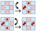
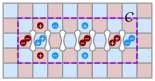
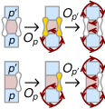
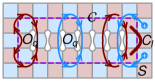
Figure 2: (Color online.) $(\vbox{\hbox{\includegraphics[height=9.0pt]{fig_ep.pdf}}},\vbox{\hbox{\includegraphics[height=9.0pt]{fig_em.pdf}}},\vbox{\hbox{\includegraphics[height=9.0pt]{fig_mp.pdf}}},\vbox{\hbox{\includegraphics[height=9.0pt]{fig_mm.pdf}}})\equiv(e,\bar{e},m,\bar{m})$ represent the $\mathbb{Z}_{N}$ charges. 2 The on-site action of link operator $I$. 2 Turn on $I$ term along a series of links (marked by ) to condense the anyons. 2 The 2nd order perturbation paths leading to the triple-plaquette operators. Excited links in the intermediate states are marked by . 2 The triple-plaquette operators on the branch-cut and around the synthetic dislocation.

The paired charges (either electric or magnetic) can be created, annihilated or moved by the link operator $I_{l}$, as illustrated in Fig. 2. $I_{l}$ couples two $\mathbb{Z}_{N}$ rotors across the link $l$:

$$I_{l}=\frac{1}{2}\left(\vbox{\hbox{\includegraphics[height=22.0pt]{fig_Il.pdf}}}+\vbox{\hbox{\includegraphics[height=22.0pt]{fig_Ir.pdf}}}\right)=\frac{1}{2}(U_{1}V_{2}+V_{1}U_{2}).$$ (5)

Because $[U_{1}V_{2},V_{1}U_{2}]=0$, all the $N^{2}$ eigenstates of $I_{l}$ are label by both eigenvalues of $U_{1}V_{2}$ and $V_{1}U_{2}$ simultaneously, which can be used to single out a unique state on which $U_{1}V_{2}=V_{1}U_{2}=1$ (and hence $I_{l}=+1$). Therefore strong enough $-I_{l}$ term can completely quench the degrees of freedom of both rotors, by polarizing the link to $I_{l}=+1$ state. Thus if the link operators $I$ are introduced to the the $\mathbb{Z}_{N}$ plaquette model along a chain of links as in Fig. 2, i.e. $H=-\frac{1}{2}\sum_{p}O_{p}-\frac{1}{2}g\sum_{l\in\mathcal{C}}I_{l}+h.c.$, two rows of sites (in region $\mathcal{C}$) will be effectively removed in the large $g$ limit, producing synthetic dislocations that are expected to be related to the charge conjugate automorphism according to the anyon condensation picture.

To explicitly verify the above statement, we resort to the 2nd order perturbation as shown in Fig. 2, and obtain the low energy effective Hamiltonian $H_{\text{eff}}=-\frac{1}{2}\sum_{p\notin\mathcal{C}}O_{p}-1/(4g\sin^{2}\frac{\theta_{N}}{2})(\sum_{q\in\mathcal{C}}O_{q}+2\sum_{q\in\partial\mathcal{C}}O_{q})+h.c.$, with the triple-plaquette operators given by

$$\begin{split}O_{q\in\mathcal{C}}&=\vbox{\hbox{\includegraphics[height=32.0pt]{fig_ZZOl.pdf}}}=U_{1}V_{2}U_{3}V_{4},\\ O_{q\in\partial\mathcal{C}}&=\vbox{\hbox{\includegraphics[height=32.0pt]{fig_ZZOe.pdf}}}=U_{1}V_{2}U_{3}V_{4}U_{5}^{\dagger}V_{6}^{\dagger},\end{split}$$ (6)

and arranged as in Fig. 2. Because the link operator $I$ is made up of counter-oriented strings as in Eq. (5), so any link that has been excited by a plaquette operator $O_{p}$ (as depicted in Fig. 2) can only decay (non-trivially) through the action of a counter-oriented plaquette operator $O_{p^{\prime}}$ across the link. This results in the convective triple-plaquette operators in Eq. (6), which glue the opposite strings together (as exemplified by $[S,O_{q}]=0$ in Fig. 2), realizing the charge conjugate automorphism. Therefore dislocations (twisted defects) associated to the charge conjugate automorphism can be synthesized by a chain of link operators $I$.

For the $\mathbb{Z}_{N}$ plaquette model with even integer $N$, there is an additional subtlety that the effective Hamiltonian also includes the term $-\alpha\sum_{l\in\partial\mathcal{C}}C_{l}$ at both ends of the chain. $l\in\partial\mathcal{C}$ labels the parallel link right next to the leftmost (or rightmost) -link, see Fig. 2. The operator $C_{l}$ is defined on such links

$$C_{l}=\left\{\begin{array}[]{ll}\vbox{\hbox{\includegraphics[height=20.0pt]{fig_Cl.pdf}}}=(-U_{1}V_{2})^{\frac{N}{2}}&\text{at left end},\\ \vbox{\hbox{\includegraphics[height=20.0pt]{fig_Cr.pdf}}}=(-V_{1}U_{2})^{\frac{N}{2}}&\text{at right end}.\end{array}\right.$$ (7)

$C_{l}$ is also a local operator acting in the low energy subspace (not leading to any excitation of the energy $\sim g$), and must be presented in the effective Hamiltonian in general. It can be obtained through a $\frac{N}{2}$th order perturbation, which makes sense only for even integer $N$. However this even-odd effect should not matter in the large $N$ limit, as the coefficient $\alpha=(\frac{g}{2})^{-N/2+1}(\frac{N}{2})^{-2}$ gets exponentially weak.

Simply by counting the constrains, it is not hard to show that add each pair of such dislocations will increase the topologically protected ground state degeneracy by $(N/2)^{2}$ for even $N$ and by $N^{2}$ for odd $N$. So each dislocation has the quantum dimension $N/2$ (for even $N$) or $N$ (for odd $N$). The reasons are as follows. Applying $-gI_{l}$ coupling to a chain of $n$ links will quench $2n$ rotors. The rotor Hilbert space dimension is reduced by $N^{2n}$. Meanwhile in the $\mathcal{C}$ region, the original $3(n+1)$ single-plaquette operators become $(n+1)$ triple-plaquette operators. As the ground state $|\text{grnd}\rangle$ is given by the constraints $\forall_{p}:O_{p}|\text{grnd}\rangle=|\text{grnd}\rangle$, each restricts the Hilbert space dimension by a factor of $1/N$. Under strong $g$ coupling, the number of constraints is reduced by $2(n+1)$. The relaxation of constraints is faster than the reduction of rotor degrees of freedom, leading to an increase of the ground state degeneracy by $N^{2(n+1)}/N^{2n}=N^{2}$. So each dislocation is associated with the additional ground state degeneracy of $N$, hence the quantum dimension $N$. However for even integer $N$, we still have the $C_{l}$ operator around each dislocation. Because $C_{l}$ has two eigenvalues $\pm 1$, it will further reduce the degeneracy by 2, resulting in the $N/2$ quantum dimension for even integer $N$. Despite of the integer quantum dimension, the charge conjugate dislocations are also non-Abelian anyons.supplementary

Conclusion— In this work, we proposed the microscopic construction of flexible and movable synthetic dislocations by simply modifying the Hamiltonian along a line of sites or links. Two kinds of synthetic dislocations in the $\mathbb{Z}_{N}$ plaquette model were explicitly constructed: one associated to the $e$-$m$ duality, and the other associated to the charge conjugation. Both are automorphisms among the intrinsic anyons related by statistical symmetry. A systematic way to design synthetic dislocations is to condense the intrinsic anyon excitations that is left over by the automorphism along the branch-cut line. The $e$-$m$ duality (charge conjugate) dislocations can be synthesized by condensing a chain of $em$ anyon (paired charges). In principle, even more general dislocations can be synthesized by arbitrary anyon condensation. The synthetic dislocations are associated to additional topological degeneracy, and rendered as projective non-Abelian anyons. Therefore anyon condensation provides us a controllable and systematic way to generate the topologically protected ground state degeneracy in a topologically ordered system.

I Supplementary Material

In the supplementary material, we discuss the anyonic properties of the synthetic dislocations constructed in this work, including their quantum dimensions and braiding rules. Because these properties are not sensitive to the microscopic details, they can be studied in the continuous space using the loop algebra approach developed by Barkeshli, Jian and Qi BarkeshliJianQi , which can be considered as a long-wave-length effective theory of synthetic dislocations. The essential idea of loop algebra is to use non-contractable Wilson loops (closed strings of operators) to keep tract of the dislocation configurations in the system and specify the ground state Hilbert space, such that the effect of adding, removing or braiding the dislocations can all be handled by the algebraic relations among these Wilson loop operators. If we have several pairs of synthetic dislocations, we may arrange them along a line and choose the non-contractable loops like those in Fig. 3. Adding each pair of dislocations into the system will introduce two additional loops: one going around the pair, and the other connects to the last pair of dislocations. All the Wilson loop operators commute with the Hamiltonian by definition, so the ground state Hilbert space is simply a representation space (presumably irreducible) of the loop algebra. The new loops introduced by new dislocations will enlarge the representation space, and hence increase the ground state degeneracy. As has been pointed out in Ref. BarkeshliJianQi , braiding two dislocations leads to the deformation of the Wilson loops, so the ground states specified by these loops are also altered, resulting in a non-Abelian Berry phase that gives rise to the projective non-Abelian statistics of dislocations. All these general principles will be demonstrated with definite examples from $\mathbb{Z}_{N}$ plaquette model in the following.

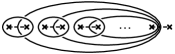
Figure 3: Non-contractable Wilson loops are chosen according to the homology basis, following Ref. BarkeshliWen .

There are two strings in the $\mathbb{Z}_{N}$ plaquette model: electric and magnetic , following the local algebra $\vbox{\hbox{\includegraphics[height=10.0pt]{appfig_Xme.pdf}}}=e^{i\theta_{N}}\vbox{\hbox{\includegraphics[height=10.0pt]{appfig_Xem.pdf}}}$ (with $\theta_{N}\equiv\frac{2\pi}{N}$), $\vbox{\hbox{\includegraphics[height=10.0pt]{appfig_Xee1.pdf}}}=\vbox{\hbox{\includegraphics[height=10.0pt]{appfig_Xee2.pdf}}}$ and $\vbox{\hbox{\includegraphics[height=10.0pt]{appfig_Xmm1.pdf}}}=\vbox{\hbox{\includegraphics[height=10.0pt]{appfig_Xmm2.pdf}}}$. Dislocations are characterized by their stabilizers (the plaquette operators at the end of the branch-cut line). According the microscopic construction, the stabilizer of $e$-$m$ duality dislocation reads $O_{q}=-e^{-i\frac{\theta_{N}}{2}}\vbox{\hbox{\includegraphics[height=18.0pt]{appfig_OOem.pdf}}}$, and the stabilizer of charge conjugate dislocation reads $O_{q}=\vbox{\hbox{\includegraphics[height=18.0pt]{appfig_OOee.pdf}}}$ or $O_{q}=\vbox{\hbox{\includegraphics[height=18.0pt]{appfig_OOmm.pdf}}}$. The ground state is given by $O_{q}=+1$, which means in the ground state manifold, we have

$$\begin{array}[]{ll}\vbox{\hbox{\includegraphics[height=18.0pt]{appfig_dis.pdf}}}=-e^{-i\frac{\theta_{N}}{2}}\vbox{\hbox{\includegraphics[height=18.0pt]{appfig_OOem.pdf}}}&\text{for $e$-$m$ duality,}\\ \vbox{\hbox{\includegraphics[height=18.0pt]{appfig_dis.pdf}}}=\vbox{\hbox{\includegraphics[height=18.0pt]{appfig_OOee.pdf}}}=\vbox{\hbox{\includegraphics[height=18.0pt]{appfig_OOmm.pdf}}}&\text{for charge conjugate.}\end{array}$$ (8)

In the following, we will focus on the case of having 4 dislocations (or 2 pairs) resting on a sphere. Denote the braiding of dislocations 1 and 2 as $\sigma_{12}$, and the braiding of 2 and 3 as $\sigma_{23}$. On the sphere, braiding 3 and 4 is equivalent to braiding 1 and 2, and thus will not be discussed.

Figure 4: (Color online.) Non-contractable Wilson loops for 4 dislocations on a sphere in the case of 4 $e$-$m$ duality dislocations, 4 charge conjugate dislocations.

We start from the $e$-$m$ duality dislocations, as shown in Fig. 4. $\mathcal{O}_{12}$ and $\mathcal{O}_{23}$ are the Wilson loops, following the algebra $\mathcal{O}_{23}\mathcal{O}_{12}=e^{i\theta_{N}}\mathcal{O}_{12}\mathcal{O}_{23}$, whose irreducible representation space is of $N$-dimension, with the basis specified by ($n=0,1,\cdots,N-1$)

$$\mathcal{O}_{12}|n\rangle=e^{in\theta_{N}}|n\rangle,\mathcal{O}_{23}|n\rangle=|n-1\rangle.$$ (9)

Because $[\mathcal{O}_{12},H]=[\mathcal{O}_{23},H]=0$, the Hamiltonian operator can be represented as $H=0$ in the representation space, thus the states $|n\rangle$ represent the degenerated ground states of the Hamiltonian. Therefore adding each pair of $e$-$m$ duality dislocations into the system will increase the ground degeneracy by a factor of $N$, hence each dislocation is of quantum dimension $\sqrt{N}$.YouWen

Braiding the dislocations will deform the Wilson loops. Under $\sigma_{12}$, $\mathcal{O}_{12}$ is not affected, however $\mathcal{O}_{23}$ undergoes the following deformation

$$\begin{split}\mathcal{O}_{23}=&\vbox{\hbox{\includegraphics[width=50.0pt]{appfig_em12_0.pdf}}}\\ \overset{\sigma_{12}}{\longrightarrow}&\vbox{\hbox{\includegraphics[width=50.0pt]{appfig_em12_1.pdf}}}\\ =&-e^{-i\frac{\theta_{N}}{2}}\vbox{\hbox{\includegraphics[width=50.0pt]{appfig_em12_2.pdf}}}\\ =&-e^{-i\frac{\theta_{N}}{2}}\vbox{\hbox{\includegraphics[width=50.0pt]{appfig_em12_3.pdf}}}\\ =&-e^{-i\frac{\theta_{N}}{2}}\vbox{\hbox{\includegraphics[width=50.0pt]{appfig_em12_4.pdf}}}\\ =&-e^{-i\frac{\theta_{N}}{2}}\mathcal{O}_{12}^{\dagger}\mathcal{O}_{23},\end{split}$$ (10)

where we have used Eq. (8) to create a stabilizer ring around the dislocation 2. Under $\sigma_{23}$, $\mathcal{O}_{23}$ is not affected, however $\mathcal{O}_{12}$ undergoes the following deformation

$$\begin{split}\mathcal{O}_{12}=&\vbox{\hbox{\includegraphics[width=50.0pt]{appfig_em23_0.pdf}}}\\ \overset{\sigma_{23}}{\longrightarrow}&\vbox{\hbox{\includegraphics[width=50.0pt]{appfig_em23_1.pdf}}}\\ =&\vbox{\hbox{\includegraphics[width=50.0pt]{appfig_em23_2.pdf}}}\\ =&-e^{-i\frac{\theta_{N}}{2}}\vbox{\hbox{\includegraphics[width=50.0pt]{appfig_em23_3.pdf}}}\\ =&-e^{-i\frac{\theta_{N}}{2}}\vbox{\hbox{\includegraphics[width=50.0pt]{appfig_em23_4.pdf}}}\\ =&-e^{-i\frac{\theta_{N}}{2}}\mathcal{O}_{23}\mathcal{O}_{12},\end{split}$$ (11)

where we have rearranged the branch-cut lines between dislocations after the braiding, and used Eq. (8) to insert the stabilizer. In summary, under the braiding of dislocations, the Wilson loops transform as

$$\begin{split}&\left\{\begin{array}[]{l}\mathcal{O}_{12}\overset{\sigma_{12}}{\longrightarrow}\mathcal{O}_{12},\\ \mathcal{O}_{23}\overset{\sigma_{12}}{\longrightarrow}-e^{-i\frac{\theta_{N}}{2}}\mathcal{O}_{12}^{\dagger}\mathcal{O}_{23},\end{array}\right.\\ &\left\{\begin{array}[]{l}\mathcal{O}_{12}\overset{\sigma_{23}}{\longrightarrow}-e^{-i\frac{\theta_{N}}{2}}\mathcal{O}_{23}\mathcal{O}_{12},\\ \mathcal{O}_{23}\overset{\sigma_{23}}{\longrightarrow}\mathcal{O}_{23}.\end{array}\right.\end{split}$$ (12)

Now we seek the unitary transform $T_{12}$ and $T_{23}$ in the ground state Hilbert space to represent $\sigma_{12}$ and $\sigma_{23}$ respectively, such that

$$\begin{split}&\left\{\begin{array}[]{l}T_{12}^{\dagger}\mathcal{O}_{12}T_{12}=\mathcal{O}_{12},\\ T_{12}^{\dagger}\mathcal{O}_{23}T_{12}=-e^{-i\frac{\theta_{N}}{2}}\mathcal{O}_{12}^{\dagger}\mathcal{O}_{23},\end{array}\right.\\ &\left\{\begin{array}[]{l}T_{23}^{\dagger}\mathcal{O}_{12}T_{23}=-e^{-i\frac{\theta_{N}}{2}}\mathcal{O}_{23}\mathcal{O}_{12},\\ T_{23}^{\dagger}\mathcal{O}_{23}T_{23}=\mathcal{O}_{23}.\end{array}\right.\end{split}$$ (13)

Given the representation of $\mathcal{O}_{12}$ and $\mathcal{O}_{23}$ in Eq. (9), it can be verified that the following is a solution of Eq. (13), up to U(1) phase factors for both $T_{12}$ and $T_{23}$,

$$\begin{split}T_{12}&=\sum_{n}e^{i\frac{\theta_{N}}{2}n(N-n)}|n\rangle\langle n|,\\ T_{23}&=\frac{e^{-i\pi/4}}{\sqrt{N}}\sum_{n,n^{\prime}}e^{i\frac{\theta_{N}}{2}(n-n^{\prime}-N/2)^{2}}|n\rangle\langle n^{\prime}|.\end{split}$$ (14)

One can check that $T_{12}$ and $T_{23}$ satisfy the braid group definition relation: $T_{12}T_{23}T_{12}=T_{23}T_{12}T_{23}$. As braiding the dislocations deforms the Wilson loops, the ground states defined by the deformed Wilson loops after braiding is related to the original ground states by the unitary transform $T_{ab}$, so $T_{ab}$ represents the non-Abelian Berry phase accumulated during the braiding. Because there is a U(1) phase ambiguity as Eq. (13) is symmetric under the transform $T_{ab}\to e^{i\theta_{ab}}T_{ab}$, hence the braid group definition relation only holds up to a U(1) phase $e^{i\phi}$, i.e. $T_{12}T_{23}T_{12}=e^{i\phi}T_{23}T_{12}T_{23}$, so the dislocations are projective non-Abelian anyons.

We continue to consider the charge conjugate dislocations, as shown in Fig. 4. Adding each pair of such dislocations will introduce four non-contractible Wilson loops: $\mathcal{O}_{12}^{e}$, $\mathcal{O}_{23}^{e}$ of electric type, and $\mathcal{O}_{12}^{m}$, $\mathcal{O}_{23}^{m}$ of magnetic type. They can be separated into two independent sets of algebra $\mathcal{O}_{23}^{m}\mathcal{O}_{12}^{e}=e^{2i\theta_{N}}\mathcal{O}_{12}^{e}\mathcal{O}_{23}^{m}$, $\mathcal{O}_{23}^{e}\mathcal{O}_{12}^{m}=e^{2i\theta_{N}}\mathcal{O}_{12}^{m}\mathcal{O}_{23}^{e}$ and $[\mathcal{O}_{12}^{e},\mathcal{O}_{23}^{e}]=[\mathcal{O}_{12}^{m},\mathcal{O}_{23}^{m}]=[\mathcal{O}_{12}^{e},\mathcal{O}_{12}^{m}]=[\mathcal{O}_{23}^{e},\mathcal{O}_{23}^{m}]=0$. If we use the common eigenstates of $\mathcal{O}_{12}^{e}$ and $\mathcal{O}_{12}^{m}$ as the basis of the ground state Hilbert space

$$\begin{split}\mathcal{O}_{12}^{e}|n_{e},n_{m}\rangle&=e^{in_{e}\theta_{N}}|n_{e},n_{m}\rangle,\\ \mathcal{O}_{12}^{m}|n_{e},n_{m}\rangle&=e^{in_{m}\theta_{N}}|n_{e},n_{m}\rangle,\end{split}$$ (15)

where $n_{e}$ and $n_{m}$ are two integers introduced to label the ground states, then $\mathcal{O}_{23}^{m(e)}$ simply lowers the index $n_{e(m)}$ by 2 (modulo $N$) according to the algebraic relations mentioned above

$$\begin{split}\mathcal{O}_{23}^{m}|n_{e},n_{m}\rangle&=|n_{e}-2,n_{m}\rangle,\\ \mathcal{O}_{23}^{e}|n_{e},n_{m}\rangle&=|n_{e},n_{m}-2\rangle.\end{split}$$ (16)

At this point it becomes obvious why the parity of $N$ is important. If $N$ is even, starting from a $n_{e}=0$ state, the operator $\mathcal{O}_{23}^{m}$ can only take it to the states labeled by even integer $n_{e}$ between 0 and $N-2$, i.e. $n_{e}=0,2,4,\cdots,(N-2)$. However if $N$ is odd, then all the states with integer $n_{e}$ between 0 and $N-1$ can be achieved by acting $\mathcal{O}_{23}^{m}$, i.e. $n_{e}=0,2,4,\cdots,(N-1),1,3,5,\cdots,(N-2)$. So for even integer $N$, both $n_{e}$ and $n_{m}$ only take $N/2$ even integer values, and the ground state Hilbert space associated to a pair of dislocations is of $(N/2)^{2}$-dimension; while for odd integer $N$, both $n_{e}$ and $n_{m}$ can take $N$ integer values, thus the associated ground state Hilbert space is of $N^{2}$-dimension. For later convenience, we introduce the notation $\llbracket N\rrbracket$

$$\llbracket N\rrbracket=\left\{\begin{array}[]{ll}N/2&\text{if $N$ even},\\ N&\text{if $N$ odd}.\end{array}\right.$$ (17)

Then the quantum dimension associated to each charge conjugate dislocation is simply $\llbracket N\rrbracket$.

Consider braiding the charge conjugate dislocations, we analyze the deformation of the $e$-loops first. The analysis of the $m$-loops will be essentially the same. Under $\sigma_{12}$, $\mathcal{O}_{12}^{e}$ is not affected, however $\mathcal{O}_{23}^{e}$ undergoes the following deformation

$$\begin{split}\mathcal{O}_{23}^{e}=&\vbox{\hbox{\includegraphics[width=50.0pt]{appfig_cc12_0.pdf}}}\\ \overset{\sigma_{12}}{\longrightarrow}&\vbox{\hbox{\includegraphics[width=50.0pt]{appfig_cc12_1.pdf}}}\\ =&\vbox{\hbox{\includegraphics[width=50.0pt]{appfig_cc12_2.pdf}}}\\ =&\vbox{\hbox{\includegraphics[width=50.0pt]{appfig_cc12_3.pdf}}}\\ =&\mathcal{O}_{12}^{e}\mathcal{O}_{23}^{e},\end{split}$$ (18)

where the stabilizer is inserted according to Eq. (8). Under $\sigma_{23}$, $\mathcal{O}_{23}^{e}$ is not affected, however $\mathcal{O}_{12}$ undergoes the following deformation,

$$\begin{split}\mathcal{O}_{12}^{e}=&\vbox{\hbox{\includegraphics[width=50.0pt]{appfig_cc23_0.pdf}}}\\ \overset{\sigma_{23}}{\longrightarrow}&\vbox{\hbox{\includegraphics[width=50.0pt]{appfig_cc23_1.pdf}}}\\ =&\vbox{\hbox{\includegraphics[width=50.0pt]{appfig_cc23_2.pdf}}}\\ =&\vbox{\hbox{\includegraphics[width=50.0pt]{appfig_cc23_3.pdf}}}\\ =&\vbox{\hbox{\includegraphics[width=50.0pt]{appfig_cc23_4.pdf}}}\\ =&\mathcal{O}_{23}^{e\dagger}\mathcal{O}_{12}^{e},\end{split}$$ (19)

where we have rearranged the branch-cut lines between dislocations after the braiding, and used Eq. (8) to insert the stabilizer. The $m$-loops deforms in the same way as $e$-loops, and will not be elaborated again. In summary, under the braiding of dislocations, the Wilson loops transform as

$$\begin{split}&\left\{\begin{array}[]{l}\mathcal{O}_{12}^{e(m)}\overset{\sigma_{12}}{\longrightarrow}\mathcal{O}_{12}^{e(m)},\\ \mathcal{O}_{23}^{e(m)}\overset{\sigma_{12}}{\longrightarrow}\mathcal{O}_{12}^{e(m)}\mathcal{O}_{23}^{e(m)},\end{array}\right.\\ &\left\{\begin{array}[]{l}\mathcal{O}_{12}^{e(m)}\overset{\sigma_{23}}{\longrightarrow}\mathcal{O}_{23}^{e(m)\dagger}\mathcal{O}_{12}^{e(m)},\\ \mathcal{O}_{23}^{e(m)}\overset{\sigma_{23}}{\longrightarrow}\mathcal{O}_{23}^{e(m)}.\end{array}\right.\end{split}$$ (20)

Again we seek the unitary transform $T_{12}$ and $T_{23}$ in the ground state Hilbert space to represent $\sigma_{12}$ and $\sigma_{23}$ respectively, such that

$$\begin{split}&\left\{\begin{array}[]{l}T_{12}^{\dagger}\mathcal{O}_{12}^{e(m)}T_{12}=\mathcal{O}_{12}^{e(m)},\\ T_{12}^{\dagger}\mathcal{O}_{23}^{e(m)}T_{12}=\mathcal{O}_{12}^{e(m)}\mathcal{O}_{23}^{e(m)},\end{array}\right.\\ &\left\{\begin{array}[]{l}T_{23}^{\dagger}\mathcal{O}_{12}^{e(m)}T_{23}=\mathcal{O}_{23}^{e(m)\dagger}\mathcal{O}_{12}^{e(m)},\\ T_{23}^{\dagger}\mathcal{O}_{23}^{e(m)}T_{23}=\mathcal{O}_{23}^{e(m)}.\end{array}\right.\end{split}$$ (21)

Note that the above equations should hold for both $\mathcal{O}_{ab}^{e}$ and $\mathcal{O}_{ab}^{m}$ simultaneously. Given the representation of $O_{ab}^{e(m)}$ in Eq. (15,16), it is easy to show that the following is a solution of Eq. (21), up to U(1) phase factors,

$$\begin{split}T_{12}&=\sum_{n_{e},n_{m}}e^{in_{e}n_{m}\theta_{N}/2}|n_{e},n_{m}\rangle\langle n_{e},n_{m}|,\\ T_{23}&=\frac{1}{\llbracket N\rrbracket}\sum_{n_{e},n_{m},n_{e}^{\prime},n_{m}^{\prime}}e^{-i(n_{e}-n_{e}^{\prime})(n_{m}-n_{m}^{\prime})\theta_{N}/2}\\ &\hskip 90.0pt|n_{e},n_{m}\rangle\langle n_{e}^{\prime},n_{m}^{\prime}|.\end{split}$$ (22)

To avoid complicated piecewise formulation of the even-odd effect, $n_{e},n_{m},n_{e}^{\prime},n_{m}^{\prime}$ should take their values from $0,2,4,\cdots,2(\llbracket N\rrbracket-1)$. For example, if $N=5$, then $n_{e(m)}^{(\prime)}=0,2,4,6,8$; and if $N=6$, then $n_{e(m)}^{(\prime)}=0,2,4$. The state $|n_{e},n_{m}\rangle$ should be understood as $|n_{e}\mod N,n_{m}\mod N\rangle$ (under modulo $N$). Then Eq. (22) is applicable to both even and odd $N$. One can check that $T_{12}$ and $T_{23}$ satisfy the braid group definition relation: $T_{12}T_{23}T_{12}=T_{23}T_{12}T_{23}$. Thus $T_{ab}$ is the non-Abelian Berry phase (upto a U(1) phase) accumulated during the braiding of dislocations $a$ and $b$. Therefore the charge conjugate dislocations are also projective non-Abelian anyons.