On Absorption by Circumstellar Dust,
With the Progenitor of SN 2012aw as a Case Study

Abstract

We use the progenitor of SN 2012aw to illustrate the consequences of modeling circumstellar dust using Galactic (interstellar) extinction laws that (1) ignore dust emission in the near-IR and beyond; (2) average over dust compositions, and (3) mis-characterize the optical/UV absorption by assuming that scattered photons are lost to the observer. The primary consequences for the progenitor of SN 2012aw are that both the luminosity and the absorption are significantly over-estimated. In particular, the stellar luminosity is most likely in the range $10^{4.8}<L_{*}/L_{\odot}<10^{5.0}$ and the star was not extremely massive for a Type IIP progenitor, with $M_{*}<15M_{\odot}$. Given the properties of the circumstellar dust and the early X-ray/radio detections of SN 2012aw, the star was probably obscured by an on-going wind with $\dot{M}\sim 10^{-5.5}$ to $10^{-5.0}M_{\odot}$/year at the time of the explosion, roughly consistent with the expected mass loss rates for a star of its temperature ($T_{*}\simeq 3600_{-200}^{+300}$ K) and luminosity. In the spirit of Galactic extinction laws, we supply simple interpolation formulas for circumstellar extinction by dusty graphitic and silicate shells as a function of wavelength ($\lambda\geq 0.3\mu$m) and total (absorption plus scattering) V-band optical depth ($\tau_{V}\leq 20$). These do not include the contributions of dust emission, but provide a simple, physical alternative to incorrectly using interstellar extinction laws.

1 Introduction

A key component to understanding supernovae (SNe) is the mapping between the explosions and their progenitor stars. Slow, steady progress is being made, and it is now well established that Type IIP SN are associated with red supergiants (see the review by Smartt 2009). There is a puzzle, however, in that the observed upper limit of $\sim 16M_{\odot}$ on the masses Type IIP SN progenitors appears to be significantly lower than the maximum masses of $\sim 25M_{\odot}$ for stars expected to explode while still red supergiants (Smartt et al. 2009), part of a more general absence of massive SN progenitors (see Kochanek et al. 2008). Since these “missing” progenitors should be more luminous than those which are being discovered, they must either be hidden, evolve differently than expected, or fail to explode. For example, in the rotating models of Ekström et al. (2012), the upper mass limit for red supergiants is lower, with $20M_{\odot}$ stars being blue rather than red at the onset of carbon burning. Alternatively, O’Connor & Ott (2011) and Ugliano et al. (2012) find that the progenitor masses of $20$-$25M_{\odot}$ corresponding to the upper mass range for red supergiants are more prone to failed explosions and prompt black hole formation, and such events would have to be found by searching for stars disappearing rather than explosions appearing (Kochanek et al. 2008). Binary evolution can also alter the distribution of final states at the time of explosion given the high probability for mass transfer as stars expand to become red supergiants (e.g. Sana et al. 2012).

If the discrepancy is not explained by the physics of stellar evolution or explosion, then the most likely remaining explanation is the effect of circumstellar dust. For example, Walmswell & Eldridge (2012) note that more massive and luminous red supergiants have stronger winds which can form dust and partly obscure the star. This then biases (in particular) the upper mass limits associated with failed searches for progenitor stars, since the luminosity limits must be corrected for an unknown amount of circumstellar dust extinction. Fraser et al. (2012) and Van Dyk et al. (2012) recently analyzed the progenitor of SN 2012aw, finding that it was both relatively high mass ($15$-$20M_{\odot}$ for Van Dyk et al. (2012) and $14$-$26M_{\odot}$ for Fraser et al. (2012)) and the most heavily obscured of any SN progenitor other than the completely obscured (and debated) SN 2008S class (see Prieto et al. 2008, Thompson et al. 2009, Kochanek 2011). Since most of the extinction vanished after the SN, the dust must have been circumstellar (Fraser et al. 2012, Van Dyk et al. 2012).

Like most studies of circumstellar dust in supernovae or supernovae progenitors, Walmswell & Eldridge (2012), Fraser et al. (2012) and Van Dyk et al. (2012) treat circumstellar dust as if it is a foreground screen that can be quantitatively modeled using Galactic interstellar extinction curve models parametrized by the value of $R_{V}$ (e.g. Cardelli et al. 1989). Usually only studies that are self-consistently calculating emission by the dust correctly model the absorption by circumstellar dust (e.g. studies of the SN 2008S class of transients by Wesson et al. 2010, Kochanek 2011, or Szczygieł et al. 2012). But three well-known effects mean that it is never appropriate to make this approximation unless the optical depth is negligible compared to the required precision of the analysis. First, emission from circumstellar dust can be important in the near-IR if the star is presently forming dust at temperatures of $1000$-$2000$ K. This matters most for hotter stars with less intrinsic near-IR emission than the red supergiants we consider here. Second, interstellar dust has the average composition of dust from all sources, while individual stars have the dust associated with their particular chemistry. This is relevant here because $\sim 20M_{\odot}$ stars generally produce silicate rather than graphitic dusts (e.g. Verhoelst et al. 2009).

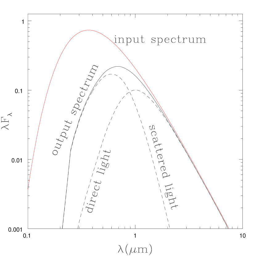
Figure 1: DUSTY model of a $10^{4}$ K black body surrounded by $\tau_{V}=3$ of cold silicate dust in a shell with $R_{out}/R_{in}=2$ and $\rho\propto 1/r^{2}$ in the shell. The dust converts the input spectral energy distribution (SED) to the output SED, where the output SED is comprised of contributions from photons that escape without scattering (direct light) and photons that escape after being scattered (scattered light). In an image, the direct emission is a point source and the scattered emission is a halo with a radius comparable to the inner radius of the shell. If the dusty shell is large enough to be resolved, only the direct emission is measured as coming from the source. We have made the dust cold enough to have no contributions from dust emission over this wavelength range.

Figure 2: Effective extinction laws $R_{\lambda}$ if the dust is a foreground screen where we only measure the unscattered direct light. The solid curves show the results for $\tau_{V}=3$ of graphitic dust (top), silicate dust (bottom) and a 50:50 mix (middle). The dashed curves show the Cardelli et al. (1989) extinction laws (CCM) with $R_{V}=4$ (top), $3.1$ (middle) and $2.0$ (bottom). Normal Galactic dust ($R_{V}=3.1$) is relatively well modeled by the 50:50 mix.

Figure 3: Effective extinction laws $R_{\lambda}$ for dust in an unresolved shell around the star where we measure both the direct and scattered light. The solid curves show the results for $\tau_{V}=3$ of graphitic dust (top), silicate dust (bottom) and a 50:50 mix (middle). The dashed curves show the best fit CCM (Cardelli et al. 1989) extinction laws with $R_{V}=2.4$ (top, graphitic), $R_{V}=2.1$ (middle, 50:50 mix) and $R_{V}=1.6$ (bottom, silicate). The fits are never very good, particularly at high optical depth, and the best fit parameters vary somewhat with the optical depth and wavelength. Goobar (2008) obtained similar results. The peak at long wavelengths (small $\lambda^{-1}$) is a silicate emission feature which DUSTY includes in the scattered light contribution to the emerging spectrum.

The third, and least appreciated point, is the different role of scattered photons in interstellar and circumstellar extinction. This issue has been discussed in detail by Wang (2005) and Goobar (2008) in the context of anomalously low estimates of $R_{V}$ for Type Ia SN, but correctly treating the problem has not become a matter of practice. For a foreground screen, scattered light forms a very diffuse, extended halo around the source which is not included in the estimate of the source flux. This halo can sometimes be seen as the extended dust echoes of transient sources (e.g. Sugerman & Crotts 2002). If the circumstellar dust is unresolved, however, the scattered light is simply included in the total flux. Thus, for interstellar extinction you observe only the direct, unabsorbed and unscattered emission, while for circumstellar extinction you observe both the direct unabsorbed and the scattered emission. Most of the observed optical emission from a moderately self-obscured star is scattered light.

Fig. 1 shows an example generated by DUSTY (Ivezić & Elitzur 1997, Ivezić et al. 1999, Elitzur & Ivezić 2001) using the spectral energy distribution (SED) of a $10^{4}$ K black body surrounded by $\tau_{V}=3$ (scattering plus absorption) of cold silicate dust. The dusty material has a density profile of $\rho\propto 1/r^{2}$ in a shell with $R_{out}/R_{in}=2$. Galactic (interstellar) extinction corresponds to putting the dust at such a large radius that we no longer include the scattered light in the observed flux of the star, and the extinction law corresponds to the wavelength dependent difference between the input spectrum and the directly escaping spectrum. Fig. 2 shows this ratio converted into an extinction law $R_{\lambda}$ for pure graphitic, pure silicate and a 50:50 mix of the two, as compared to Cardelli et al. (1989) Galactic extinction laws with $R_{V}=4.0$, $3.1$ and $2.0$. Galactic dust models typically have a roughly 50:50 mix of graphitic and silicate grains (see the summary in Draine 2011), and using this mix in the DUSTY models roughly reproduces a typical $R_{V}=3.1$ Galactic extinction law. The match is not perfect because there are differences in the assumed size distributions.

For a star surrounded by an unresolved shell of dust, however, the emission we measure is the sum of the direct and scattered light, which is very different from the direct emission alone. Fig. 3 shows this case converted into an effective circumstellar extinction law for the same three dust mixtures. For circumstellar dust, all three examples are now significantly below the $R_{V}=3.1$ curve and a given change in color implies a significantly smaller change in luminosity. If we fit the absorption in these DUSTY models with Cardelli et al. (1989) extinction models, the best fits for the graphitic, silicate and 50:50 dusts are $R_{V}\simeq 2.4$, $R_{V}\simeq 1.6$ and $R_{V}\simeq 2.1$, respectively. These are the best fits for $\tau_{V}=3$ from $0.36\mu$m (U band) to $1\mu$m. The best fits vary modestly ($\Delta R_{V}\simeq 0.1$) with $\tau_{V}$ and the fitted wavelength range, become worse for higher optical depths, and there are no truly good fits. Fig. 3 superposes these Cardelli et al. (1989) extinction curves on the DUSTY models. Goobar (2008) found similar estimates for the best Cardelli et al. (1989) extinction curves to model circumstellar dust and also noted that they are not very good approximations.

The final point to note in Figs. 2 and 3 is that the dust composition is quantitatively important. Interstellar dust is a mixture of graphitic and silicate dusts from many sources. Individual stars, however, typically only produce silicate or graphitic dusts depending on the carbon to oxygen abundance ratio of the stellar atmosphere. To zeroth order, all available carbon and oxygen bond to make CO. Then, a carbon poor (rich) atmosphere has excess oxygen (carbon) to make silicate (graphitic) dusts. The atmospheres of $\sim 20M_{\odot}$ red supergiants usually form silicate dusts (e.g. Verhoelst et al. 2009) because they never undergo the dredge up phases that enrich the atmospheres of the lower mass AGB stars with carbon (e.g. Iben & Renzini 1983). Assuming a mixed interstellar composition will generally overestimate the absorption associated with a given change in color for silicate dusts and underestimate it for graphitic dusts.

In this paper we consider the effects of dust on the progenitor of SN 2012aw in more detail. First, in §2 we use archival Spitzer IRAC data to set stringent limits on the 3.6, 4.5, 5.8 and $8.0\mu$m fluxes of the progenitor, and then model the spectral energy distribution (SED) of the progenitor with DUSTY in order to correctly model absorption, scattering and emission from a dust enshrouded star. We highlight where any extinction law derived for dust screens at great distances from the source such as the standard Cardelli et al. (1989) extinction laws can create problems. Finally, in §3 we summarize the results and provide simple interpolation formulas for extinction by graphitic and silicate circumstellar dust as a function of wavelength and optical depth.

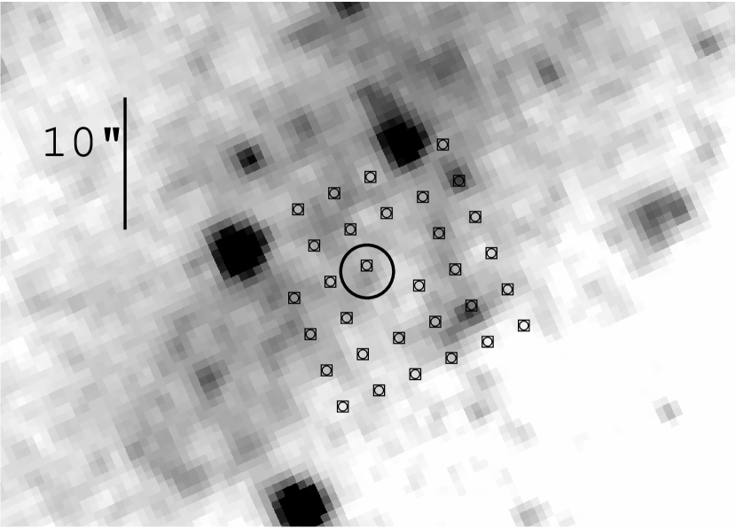
Figure 4: Combined $3.6$ and $4.5\mu$m images of the region surrounding the progenitor of SN 2012aw. The 2$\farcs$0 diameter circle marks the estimated position of the progenitor, although the formal uncertainties in the position are far smaller ($0\farcs 05$). The smaller points show the grid of apertures used to estimate the flux limits, where missing points show the locations of dropped apertures (see text). A few of the grid points lie near fainter sources that are obvious in this co-added image but only marginally detectable (at about $2\sigma$) in the four individual images combined to make Fig. 4. The image is aligned to the world coordinate system with North up and East left.

2 Mid-IR Flux Limits, X-ray Fluxes and Models

As noted by Fraser et al. (2012), there are no obvious sources in the archival SINGS (Kennicutt et al. 2003) IRAC images of the region around the progenitor. It is, however, a relatively clean region with the emission dominated by unresolved stars, as shown in Fig. 4. We identified 8 nearby stars in common between the HST I-band image used by Fraser et al. (2012) and Van Dyk et al. (2012) to identify the progenitor and the image formed by co-adding the $3.6$ and $4.5\mu$m data and used the IRAF geomap/geotran scripts to estimate the position of the progenitor shown in Fig. 4. Based on jackknife resampling of the reference stars, the nominal uncertainties in the position are small (about 0$\farcs$05).

Since we are essentially confusion limited, we estimated flux limits using the grid of 36 apertures covering the location of the progenitor and bounded by the nearby brighter stars as shown in Fig. 4. The grid spacing was 3$\farcs$0. We used the IRAF APPHOT/PHOT to measure aperture magnitudes with a signal radius of 2$\farcs$4 and a sky annulus from 2$\farcs$4 to 7$\farcs$2. The fluxes were calibrated following the procedures given in the Spitzer Data Analysis Cookbook and aperture corrections of 1.213, 1.234, 1.379, and 1.584 for the 3.6 through $8.0\mu$m bands. Keeping the sky annulus immediately next to the signal aperture minimizes the effects of background variations created by the galaxy. We used a $2\sigma$ outlier rejection procedure in order to exclude sources located in the local sky annulus, and correct for the excluded pixels assuming a Gaussian background flux distribution.

We clipped 3 of the grid points in the wings of the brighter sources and the two lowest (negative) flux points that lay in an obvious “dark lane”, leaving 31 points. Based on one of the two SINGS epochs, the variances in the four bands are $10.7$, $11.4$, $12.8$ and $14.2$ $\mu$Jy for the $3.6$, $4.5$, $5.8$, and $8.0\mu$m bands respectively. This is well above the nominal noise level for the exposure time ($0.5$, $0.8$, $6$, and $6$ $\mu$Jy) because there is stellar emission in the region. The variance after coadding the two SINGS epochs is only slightly smaller, as expected for noise dominated by confusion, so we rather conservatively use the variances derived from the single epoch as $1\sigma$ flux limits. Note that some of the grid points clearly lie on sources in the coadded image. These sources are not readily apparent in the four individual sub-images, where their detection significance would be roughly $2\sigma$. A source of similar flux at the supernova position would be equally obvious in Fig. 4.

For models of the spectral energy distribution, we combined the V and I band estimates from Van Dyk et al. (2012) and Fraser et al. (2012), including the difference in their V-band estimates as an additional systematic error. We used the J and K_s estimates from Van Dyk et al. (2012), based on their better photometric calibrations. We use a minimum flux uncertainty of 20%, which broadens the V, I and J-band photometric errors, given that the data were obtained over a long time period (1994-2009, with the SINGS IRAC data being obtained on 22/23 May 2004) and Van Dyk et al. (2012) argue for the detection of variability at V and I. We model the star using the MARCS (Gustafsson et al. 2008) stellar atmosphere models, considering only the $15M_{\odot}$, solar metallicity, $5$ km/s turbulent velocity $\log_{10}g=-0.5$ models preferred by Van Dyk et al. (2012) and also considered by Fraser et al. (2012). These are available for effective temperatures of $T_{e}=3300$ to $4000$ K in steps of $100$ K and then $4250$ and $4400$ K. For intermediate temperatures we linearly interpolate between the available models. We averaged the high resolution MARCS models and the filter transmission functions onto a coarser wavelength grid for use in the DUSTY models and then generated magnitude estimates for each model including the appropriate averages over the filter band passes. We first fit the measurements to normalize the luminosity, and then added a contribution from the upper limits as $\Delta\chi^{2}=(F_{model}/F_{limit})^{2}$ for each band, where $F_{model}$ is the estimate from the normalized model and $F_{limit}$ is the $1\sigma$ limit on the flux.

Immler & Brown (2012) reported a Swift (Gehrels et al. 2004) X-ray detection of the SN in the first week and Stockdale et al. (2012) and Yadav et al. (2012) report $20$ GHz radio detections in the first month. Swift continued to monitor the SN for an extended period, so as an independent probe of the circumstellar medium we obtained all the archival Swift XRT data, binning the observations as summarized in Table 1. We reprocessed the XRT data using the xrtpipeline tool provided by the Swift team. We binned the observations into six roughly logarithmic time intervals and then reprojected each group of observations into a single image. We chose the source region to be a circle centered on the SN with a radius of 10 pixels (23$\farcs$6) and a nearby background region without any sources, using aperture corrections based on the analysis of the Swift PSF by Moretti et al. (2005). Following Immler & Brown (2012) we assumed a Galactic foreground column density of $2.9\times 10^{20}$ (Dickey & Lockman 1990). For our epoch best matching Immler & Brown (2012) we reproduce their count rates. While none of the X-ray detections are of very high significance, there appears to be a low level of detectable ($3\sigma$) and probably time varying X-ray emission for the first 1–2 months. There are no clear detections at low energies ($0.2$–$0.5$ keV) and only very marginal detections at high energies ($2$–$10$ keV) – the observed counts are completely dominated by the $0.5$–$2$ keV band.

We use the DUSTY (Ivezić & Elitzur 1997, Ivezić et al. 1999, Elitzur & Ivezić 2001) dust radiation transfer models to correctly include dust emission, absorption, scattering and composition when modeling the progenitor SED. We use either graphitic or silicate dust models from Draine & Lee (1984) and the default Mathis et al. (1977) power-law grain size distribution ($dn/da\propto a^{-3.5}$ for $0.005\mu\hbox{m}<a<0.25\mu\hbox{m}$). The dust lies in a spherical shell with a $1/r^{2}$ density distribution and a $R_{out}/R_{in}=10$ axis ratio between the inner and outer radii. While the directly escaping light depends only on the optical depth, thicker shells (larger $R_{out}/R_{in}$) allow more scattered light to escape than thin shells for the same total optical depth, but this is a second order effect and we will hold $R_{out}/R_{in}$ fixed. The model parameters are the luminosity of the star, $L_{*}$, the temperature of the star, $T_{*}$, the temperature $T_{d}$ of the dust at $R_{in}$, and the dust optical depth $\tau_{V}$ at V-band ($0.55\mu$m). This is the total (absorption plus scattering) optical depth, $\tau_{tot}=\tau_{abs}+\tau_{scat}$, where the scattering optical depth is related to the total optical depth by the albedo, $\tau_{scat}=w\tau_{tot}$. The effective absorption optical depth is approximately $\tau_{e}=(\tau_{tot}\tau_{abs})^{1/2}=(1-w)^{1/2}\tau_{tot}$. At V-band, the standard DUSTY silicate (graphitic) dust models have albedos of $w_{V}=0.86$ ($0.47$), so for the same effective absorption the silicate models require significantly higher total optical depths $\tau_{V}$. The V-band extinction is approximately $A_{V}=2.5\tau_{e,V}/\ln 10=0.41\tau_{V}$ ($0.79\tau_{V}$) for the silicate (graphitic) model. The radius $R_{in}$ is then a derived quantity given the model parameters. We fit the data and estimate uncertainties by embedding DUSTY in a Markov Chain Monte Carlo (MCMC) driver. Without mid-IR detections, we cannot determine the dust temperature, so we simply considered cases with $T_{d}=100$ K, $500$ K, $1000$ K and $1500$ K. We assume a fixed foreground Galactic extinction of $E(B-V)=0.05$ mag (modeled using an $R_{V}=3.1$ extinction law) and a distance modulus of $\mu=30$ mag (Freedman et al. 2001).

While they are not physically correct models, we do recover the results of Van Dyk et al. (2012) and Fraser et al. (2012) if we model our version of the SED including the mid-IR flux limits but no dust emission and using Cardelli et al. (1989) extinction laws. Like Van Dyk et al. (2012) we find that higher $R_{V}$ extinction laws provide better fits, but we also find a stellar temperature degeneracy similar to Fraser et al. (2012). Clearly the models have a “degeneracy” direction which is very sensitive to the exact assumptions of the model and can lead to either tight or loose limits on the effective temperature. The specific rationale for using $R_{V}\simeq 4$ extinction laws in Van Dyk et al. (2012) is not really valid, but allowing freedom in the extinction curve is certainly a more conservative approach. For example, if we fix $R_{V}=4.35$ and $T_{*}=3600$ K to match Van Dyk et al. (2012), we obtain a luminosity of $\log_{10}L_{*}/L_{\odot}=5.15\pm 0.05$ compared to $5.21\pm 0.03$. If we fix $R_{V}=3.1$ to match Fraser et al. (2012), then we find $\log_{10}L_{*}/L_{\odot}=5.10\pm 0.05$ for $T_{*}=3600$ K and $\log_{10}L_{*}/L_{\odot}=5.43\pm 0.05$ for $T_{*}=4400$ K, close the values of $\log_{10}L_{*}/L_{\odot}=5.0$ and $5.6$ they find for temperatures of $T_{*}=3550$ K and $4450$ K using MARCS models with $\log_{10}g=0$.

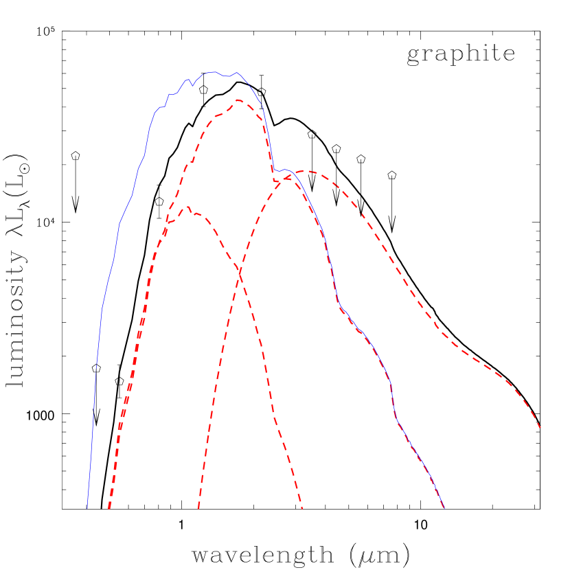
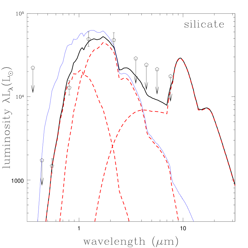
Figure 5: Graphitic (top) and silicate (bottom) fits to the SED of the progenitor for $T_{d}=1000$ K at the inner edge of the dust distribution. The heavy black curves show the SED model, which is comprised of (from left to right) scattered, direct and dust emission, as shown by the dashed red curves. The thin blue curves show the model for the unobscured SED of the star. The open symbols show the measured luminosities and limits. Note the different balance between absorption and scattering for the two dust compositions and the modest contribution of dust emission to the K_s band.

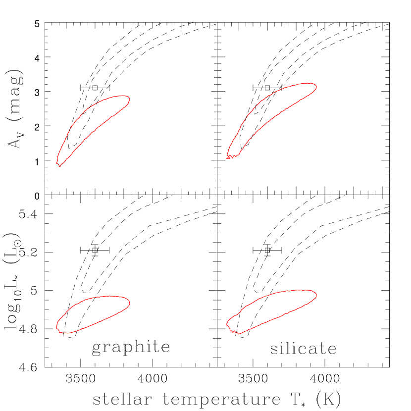
Figure 6: Constraints on the visual extinction $A_{V}$ (top) and stellar luminosity $L_{*}$ (bottom) as a function of stellar temperature $T_{*}$. The solid contours show the $1\sigma$ constraints on two parameters ($\Delta\chi^{2}=2.3$) for the graphitic (left) and silicate (right) models and an inner edge dust temperature of $T_{d}=1000$ K roughly corresponding to having a dust forming wind at the time of the observations. The points and dashed contours show the results from Van Dyk et al. (2012) and Fraser et al. (2012), respectively. The DUSTY model $\tau_{V}$ were converted to $A_{V}=2.5(1-w_{V})^{1/2}\tau_{V}/\ln 10$.

Fig. 5 shows two representative DUSTY models of the progenitor for circumstellar silicate and graphitic dusts with $T_{d}=1000$ K, roughly corresponding to the expected inner edge dust temperatures if the star was forming dust at the time of the observations. Formally, the graphitic model is a better fit ($\chi^{2}=5.5$ versus $8.8$), but the models have essentially identical stellar luminosities, $L_{*}=10^{4.9}L_{\odot}$, and temperatures, $T_{*}\simeq 3550$ K. Both models marginally satisfy the mid-IR flux limits at this luminosity, with the graphitic models primarily limited by the non-detections at $3.6$ and $4.5\mu$m, and the silicate models limited by the contribution of silicate emission peak at $8.0\mu$m.

Fig. 5 illustrates all three of the basic points about circumstellar dust as compared to interstellar dust. First, the optical flux is completely dominated by the scattered emission that is not included in interstellar extinction laws. Second, dust emission is quantitatively important to the K_s band flux. Because the star is cold, dust emission does not dominate the near-IR flux as it would for a hot star of the same luminosity and degree of obscuration, but it does partly compensate for the absorption. Third, there are quantitative differences between the two dust types in their balance between absorption and scattering and the nature of the mid-IR emission. The total optical depths of the models are quite different, $\tau_{V}=5.9$ for silicates and $\tau_{V}=2.6$ for graphite, but the effective absorption optical depths of the two models are very similar, with $\tau_{e,V}=(1-w_{V})^{1/2}\tau_{V}=2.2$ for silicates and $1.9$ for graphite.

Fig. 6 shows the allowed parameter ranges for the stellar luminosity $L_{*}$ and visual extinction $A_{V}$ as a function of stellar temperature $T_{*}$ as compared to the results from Fraser et al. (2012) and Van Dyk et al. (2012). We show the results for $T_{d}=1000$ K, which roughly corresponds to the inner edge dust temperature if there was a dust forming wind at the time of the observations. Table 2 gives the results for the other dust temperatures. They are generally similar except for the $T_{d}=100$ K graphitic model. The key issue for the progenitor is that the preferred solutions of both Fraser et al. (2012) and Van Dyk et al. (2012) significantly overestimate the luminosity of the progenitor. Our results agree with Van Dyk et al. (2012) on the temperature, but the luminosity $L_{*}$ is a factor of two lower. The mid-IR limits essentially preclude the higher luminosity and temperature solutions of Fraser et al. (2012) unless the dust temperature is made significantly lower than $T_{d}=500$ K and the dust emission moves out of the IRAC band passes. Even there, only the cold $T_{d}=100$ K graphitic model allows a significantly higher luminosity. As expected, a large part of the difference is that the models based on interstellar extinction are significantly overestimating the overall absorption.

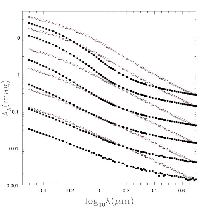
Figure 7: Extinction $A_{\lambda}$ as a function of wavelength for silicate (squares) and graphitic (triangles) circumstellar dust with $R_{out}/R_{in}=10$ and optical depths of $\tau_{V}=0.1$ (bottom), $0.3$, $1.0$, $3.0$, $10.0$ and $20.0$ (top). Note how the shapes of the curves depend on both composition and optical depth. The curves through the points are the model from Table 3.

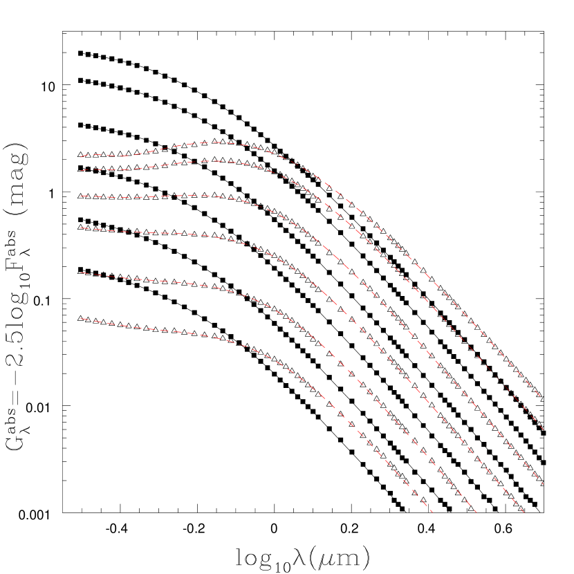
Figure 8: Interpolation function $G_{\lambda}^{abs}=-2.5\log_{10}F_{\lambda}^{abs}$ for the fraction of the observed light that is direct emission as a function of wavelength for silicate (squares) and graphitic (triangles) circumstellar dust with $R_{out}/R_{in}=10$ and optical depths of $\tau_{V}=0.1$ (bottom), $0.3$, $1.0$, $3.0$, $10.0$ and $20.0$ (top). The curves through the points are the model from Table 4. For an input SED $S_{\lambda}$, the observed SED is $S_{\lambda}10^{-0.4A_{\lambda}}$ of which $S_{\lambda}10^{-0.4A_{\lambda}}F_{\lambda}^{abs}=S_{\lambda}10^{-0.4(A_{\lambda}+G_{\lambda}^{abs})}$ is directly escaping emission and $S_{\lambda}10^{-0.4A_{\lambda}}(1-F_{\lambda}^{abs})$ is scattered emission. As in Fig. 7, note how the shapes of the curves depend on both composition and optical depth.

3 Discussion

Fraser et al. (2012) and Van Dyk et al. (2012) argue that the progenitor was probably the most massive yet found for a Type IIP SN, probably at or above the upper limit of $(16.5\pm 1.5)M_{\odot}$ Smartt et al. (2009) found in their statistical analysis of the masses of Type IIP progenitors. Given the amount of circumstellar extinction, this seemed to match the suggestion by Walmswell & Eldridge (2012) that the upper mass limit could be biased by increasing levels of dust formation for the more massive red supergiants due to the increase in mass loss rates with luminosity. Here we argue that many of these inferences are biased by incorrectly modeling circumstellar dust with an interstellar extinction law, thereby overestimating both the amount of extinction and the luminosity of the star. When we model the SED using circumstellar dust models, the luminosity of the star is $L_{*}<10^{5}L_{\odot}$ and the mass is $M_{*}<15M_{\odot}$, where the downwards shifts are easily understood from the differing physics of interstellar and circumstellar extinction. The visual extinction is overestimated because interstellar extinction neglects the contributions of scattered light, and, to a lesser extent because of the low stellar temperature, the near-IR (K_s) extinction is overestimated by neglecting the emission from hot dust. The absence of a mid-IR source noted by Fraser et al. (2012) is a key point of evidence, since there should have been a detectable source given the proposed, higher luminosities unless the dust is cold and emitting at longer wavelengths than the IRAC bands. In this particular case, the dust composition has little effect on the inferred properties of the star.

Unfortunately, without measuring the mid-IR portion of the SED we cannot determine the dust temperature $T_{d}$ other than limiting it to be lower than the dust destruction temperature ($T_{d}\simeq 1500$ K). However, the wind properties are a strong function of the dust temperature because at fixed optical depth far more mass is required if the material is at larger radii and colder temperatures. Ignoring the minor (10%) corrections from the finite value of $R_{out}/R_{in}=10$, the mass loss rate required to support the optical depth is

$$\dot{M}=4\pi R_{in}v_{w}\tau_{V}\kappa_{V}^{-1}\simeq 10^{-5}R_{in15}v_{w10}\tau_{V5}\kappa_{V100}^{-1}M_{\odot}~{}\hbox{year}^{-1}$$ (1)

where $R_{in}=10^{15}R_{in15}$ cm, $v_{w}=10v_{w10}$ km/s, $\tau_{V}=5\tau_{V5}$ and $\kappa_{V}=10^{2}\kappa_{v100}$ cm²/g. Table 2 gives the values for the individual models. Supporting $\tau_{V}\sim 5$ when $T_{d}\simeq 100$ K requires mass loss rates of order $\dot{M}\sim 10^{-2.5}M_{\odot}$/year and implies total wind masses of order $3M_{\odot}$ that are implausible for a star with an initial mass of $M_{*}<15M_{\odot}$. For comparison, the empirical approximations of de Jager et al. (1988) predict $\log_{10}(\dot{M}/M_{\odot}/\hbox{year})\simeq-5.8\pm 0.5$ for a red supergiant wind, roughly matching the rates needed if the wind is producing dust at the time of the explosion.

The density of the wind is also tied to the expected phenomenology of the explosion. If we assume the standard $\rho_{e}\propto v^{-12}$ outer ejecta density profile for red supergiants (Matzner & McKee 1999) then the expected shock velocity is

$$v_{s}=8200E_{51}^{9/20}M_{e10}^{-7/20}\dot{M}_{-4}^{-1/10}v_{w10}^{1/10}t_{1}^{-1/10}~{}\hbox{km/s}$$ (2)

(e.g. Chevalier & Fransson 2003), where the total energy of the supernova is $E=10^{51}E_{51}$ ergs, the ejected mass is $M_{e}=10M_{e10}M_{\odot}$, $\dot{M}=10^{-4}\dot{M}_{-4}M_{\odot}$/year and $t_{1}$ is the elapsed time in days. A shock expanding through a dense medium generates a luminosity of $L_{S}=(1/2)\dot{M}v_{s}^{3}/v_{w}$, which we report in Table 2 for $v_{s}=5000$ km/s and $v_{w}=10$ km/s. The emission from the forward shock is usually too hard to be easily detected, but assuming that the reverse shock is cooling and that its softer emissions dominate the observable X-ray emissions, the expected X-ray luminosity is

$$L_{x}\simeq{9\dot{M}v_{s}^{3}\over 500v_{w}}\simeq 1.63\times 10^{7}E_{51}^{27/20}M_{e10}^{-21/20}\dot{M}_{-4}^{7/10}v_{w10}^{-7/10}t_{1}^{-3/10}L_{\odot}$$ (3)

with a temperature of order 1 keV (e.g. Chevalier & Fransson 2003). If we model the X-ray fluxes in Table 1 using Eqn. 3 and a range of additional absorption from $N_{H}=10^{20}$ to $10^{23}$ cm^-2, the mass loss rates for epochs 1, 3 and 5 (which have the smallest uncertainties) are

$$\dot{M}\sim\left(10^{-6.4\pm 0.4},10^{-5.8\pm 0.3},10^{-4.7\pm 0.3}\right)v_{w10}M_{e10}^{3/2}E_{51}^{-27/14}M_{\odot}/\hbox{year},$$ (4)

respectively, with some evidence that the amount of excess absorption needed above Galactic is increasing with time. Such fluctuations and trends are not unusual (e.g. Dwarkadas & Gruszko 2012), but the X-ray emission appears to be broadly consistent with the presence of a wind with roughly the right density to explain the extinction of the progenitor. Stockdale et al. (2012) and Yadav et al. (2012) report rising $\simeq 20$ GHz radio fluxes of $0.160\pm 0.025$ and $0.315\pm 0.018$ mJy roughly 7 and 13 days after discovery that also argue for a significant wind at the time of the SN. If we model the radio emission following Soderberg et al. (2005) assuming the ejecta mass is $M_{e}=(15-1.4)M_{\odot}=13.6M_{\odot}$ and $E_{51}=1$, we obtain estimates of $\dot{M}\sim 10^{-5.0}v_{w10}M_{\odot}$/year, although given only two data points at essentially the same frequency, the models are not tightly constrained. The Thompson optical depth of the wind is always negligible, since it is a small ($\mathrel{\raise 1.29167pt\hbox{$<$}\mkern-14.0mu\lower 2.58334pt\hbox{$\sim$}}1\%$) fraction of the dust optical depth, but the cold dust solutions would likely convert the SN into a Type IIn because the H$\alpha$ luminosity from recombination is of order $3000R_{in15}L_{\odot}$ and increases linearly with the distance to the circumstellar material. Thus, while the data is fragmentary, the simplest interpretation appears to be that there was a relatively steady $\dot{M}\sim 10^{-5.5}$ to $10^{-5.0}M_{\odot}$/year wind creating the obscuration at the time of the SN.

Since the primary reason for inappropriately using Galactic extinction laws for circumstellar dust is almost certainly their ease of use, we supply in Table 3 equivalently easy to use models for absorption by circumstellar dust. The problem is somewhat more complex because the extinction depends on both wavelength and optical depth, but the absorption in the DUSTY models from the UV to mid/near-IR ($0.3\mu$m to $5.0\mu$m) can be well modeled by the functional form

$$A_{\lambda}(\tau_{V})=\tau_{V}\lambda^{-x}\sum_{i}\sum_{j}a_{ij}\tau_{V}^{i}\lambda^{-j}.$$ (5)

for optical depths up to $\tau_{V}=20$. Here $\lambda$ is the wavelength in microns and $\tau_{V}$ is the total (absorption plus scattering) optical depth in the V band. Table 3 provides these models for $R_{out}/R_{in}=2$ and $10$ in a format where they can simply be extracted from the electronic paper using a mouse and inserted into most numerical environments. The fits reproduce the DUSTY results with rms fractional residuals of 1.4% (1.6%) and 1.8% (2.2%) for the graphitic and silicate models and $R_{out}/R_{in}=10$ ($2$), although this includes some numerical rounding errors in the DUSTY models at low optical depths and longer wavelengths. They can be extrapolated to longer wavelengths relatively safely, but at these longer wavelengths one would almost always also need to include dust emission. They should not be extrapolated to shorter wavelengths or higher optical depths. Fig. 7 shows the circumstellar extinction of the DUSTY models used to build these interpolating functions and the interpolating functions as extracted from Table 3 for $R_{out}/R_{in}=10$. In some circumstances it will also be useful to separate the direct and scattered light. The fraction of the observed flux that is direct, $F_{\lambda}^{abs}$, can be well-modeled by

$$G_{\lambda}^{abs}=-2.5\log_{10}F_{\lambda}^{abs}(\tau_{V})=\tau_{V}^{1/2}(1+\lambda^{x})^{-1}\sum_{i}\sum_{j}a_{ij}\tau_{V}^{i/2}\lambda^{-j}.$$ (6)

These interpolating functions are supplied in Table 4 and the quality of the fits is shown in Fig. 8. For a source with intrinsic spectrum $S_{\lambda}$, the observed spectrum is $S_{\lambda}10^{-0.4A_{\lambda}}$, the directly escaping flux is $S_{\lambda}10^{-0.4A_{\lambda}}F_{\lambda}^{abs}=S_{\lambda}10^{-0.4(A_{\lambda}+G_{\lambda}^{abs})}$ and the escaping but scattered flux is $S_{\lambda}10^{-0.4A_{\lambda}}(1-F_{\lambda}^{abs})$. Obviously, this approach can be generalized to other dust compositions or size distributions. We parametrize the models by $\tau_{V}$ because $\tau_{V}$ is closely related to the physical properties of the wind (Eqn. 1), while relating it to a color (i.e. $E(B-V)$) would divorce the model from the underlying physics. There is no comparably simple means of treating dust emission because it depends critically on the input spectrum.

These differences are quantitative rather than qualitative – in circumstellar dust models the progenitor of SN 2012aw is still fairly heavily obscured, as found by Fraser et al. (2012) and Van Dyk et al. (2012), and Walmswell & Eldridge (2012) are correct that circumstellar dust introduces a bias that must be modeled when considering the statistics of SN progenitors, particularly when modeling non-detections in analyses like Smartt et al. (2009). However, since changes in extinction physics exponentially modify quantities like luminosities, these differences between the two dust geometries are quantitatively important. We note, however, that SN where circumstellar dust will strongly bias inferences about the progenitor have densities of circumstellar material that will lead to X-ray or radio emission, as observed for SN 2012aw, because the optical depth is proportional to the wind density. For example, combining Eqns. 1 and 3, we see that the expected X-ray luminosity is $L_{X}\propto\tau_{V}$. This means that the properties of the explosion can be used to constrain biases from dust around the progenitor even if the observations of the progenitor are inadequate to constrain the circumstellar extinction.

There are, of course, additional complexities coming from the geometry of the dust around the star that can lead to differences in the effective optical depth along the line of sight for direct emission and averaged over a significant fraction of the shell for the scattered emission. Our simple models provide two means of approximating some of these effects. First, changes in the shell thickness can be used to adjust the balance between scattered and absorbed light. Second, the emergent flux can be modeled as a sum of direct light with one optical depth, and scattered light with another in order to model differences between the mean and line-of-sight optical depths. Independent of these questions, interstellar and circumstellar extinction are quantitatively different, and in this case ignoring the differences leads to a significant overestimate of the progenitor luminosity and mass.

Table 1: Swift X-ray Data

Obsid	$\langle\hbox{Date}\rangle$	$T_{exp}$ (sec)	0.2–10 keV	0.2–0.5 keV	0.5–2 keV	2–10 keV	Range
00032319001	March 21.0	$9151$	$1.781\pm 0.536$	$0.174\pm 0.197$	$1.445\pm 0.458$	$0.162\pm 0.197$	03/21
00032319002	March 23.0	$5856$	$0.449\pm 0.376$	$-0.090\pm 0.028$	$0.369\pm 0.306$	$0.171\pm 0.217$	03/23
00032319003	March 25.0	$8843$	$1.528\pm 0.497$	$-0.053\pm 0.018$	$1.520\pm 0.475$	$0.061\pm 0.145$	03/25
00032319004–006	March 30.4	$22714$	$0.618\pm 0.229$	$0.037\pm 0.112$	$0.323\pm 0.146$	$0.261\pm 0.136$	03/28-04/01
00032315015–030	April 12.5	$48188$	$0.358\pm 0.136$	$0.117\pm 0.089$	$0.059\pm 0.058$	$0.184\pm 0.085$	04/01-04/22
00032315031–042	June 14.9	$17430$	$-0.123\pm 0.198$	$-0.302\pm 0.080$	$0.280\pm 0.164$	$-0.100\pm 0.076$	04/26-07/14

Note. — $\langle\hbox{Date}\rangle$ is the exposure time weighted average date, where Range gives the range of dates spanned by the epochs. The counts are in units of counts/ksec.

Table 2: Model Fits

Type	$T_{d}$ (K)	$\log_{10}(L_{*}/L_{\odot})$	$T_{*}$ (K)	$\log_{10}\tau_{V}$	$\log_{10}(R_{in}/\hbox{cm})$	$\log_{10}\dot{M}$	$\log_{10}(L_{s}/L_{\odot})$
sil	$100$	$4.99\hphantom{0}(4.88/5.12)$	$3754\hphantom{0}(3483/4168)$	$0.87\hphantom{0}(0.72/0.97)$	$16.97\hphantom{0}(16.84/17.10)$	$-2.85\hphantom{0}(-3.14/-2.63)$	$9.16\hphantom{0}(8.87/9.38)$
sil	$500$	$4.93\hphantom{0}(4.80/5.06)$	$3600\hphantom{0}(3357/3991)$	$0.80\hphantom{0}(0.48/0.93)$	$15.31\hphantom{0}(15.13/15.46)$	$-4.59\hphantom{0}(-5.09/-4.31)$	$7.43\hphantom{0}(6.92/7.70)$
sil	$1000$	$4.91\hphantom{0}(4.81/5.01)$	$3603\hphantom{0}(3385/3976)$	$0.79\hphantom{0}(0.55/0.91)$	$14.80\hphantom{0}(14.67/14.93)$	$-5.11\hphantom{0}(-5.48/-4.86)$	$6.90\hphantom{0}(6.53/7.15)$
sil	$1500$	$4.90\hphantom{0}(4.81/4.97)$	$3823\hphantom{0}(3473/4264)$	$0.85\hphantom{0}(0.67/0.94)$	$14.50\hphantom{0}(14.36/14.60)$	$-5.35\hphantom{0}(-5.67/-5.17)$	$6.66\hphantom{0}(6.35/6.85)$
gra	$100$	$5.14\hphantom{0}(4.96/5.30)$	$3897\hphantom{0}(3528/4308)$	$0.64\hphantom{0}(0.45/0.74)$	$17.40\hphantom{0}(17.25/17.53)$	$-2.65\hphantom{0}(-3.00/-2.43)$	$9.36\hphantom{0}(9.01/9.58)$
gra	$500$	$4.95\hphantom{0}(4.82/5.08)$	$3528\hphantom{0}(3360/3821)$	$0.44\hphantom{0}(0.13/0.60)$	$15.81\hphantom{0}(15.70/15.93)$	$-4.46\hphantom{0}(-4.87/-4.18)$	$7.56\hphantom{0}(7.14/7.84)$
gra	$1000$	$4.89\hphantom{0}(4.79/4.97)$	$3562\hphantom{0}(3372/3910)$	$0.43\hphantom{0}(0.17/0.57)$	$14.97\hphantom{0}(14.88/15.07)$	$-5.30\hphantom{0}(-5.65/-5.07)$	$6.71\hphantom{0}(6.36/6.95)$
gra	$1500$	$4.84\hphantom{0}(4.76/4.93)$	$3694\hphantom{0}(3392/4222)$	$0.48\hphantom{0}(0.16/0.61)$	$14.49\hphantom{0}(14.37/14.59)$	$-5.74\hphantom{0}(-6.17/-5.50)$	$6.28\hphantom{0}(5.84/6.51)$

Note. — These are the median and 90% confidence intervals of the MCMC results. The implied mass loss rate $\dot{M}$ is in units of $v_{w10}\kappa_{V100}^{-1}M_{\odot}/\hbox{year}$, and the shock luminosity $L_{s}$ is in units of $(v_{s}/5000\hbox{km/s})^{3}\kappa_{V100}^{-1}L_{\odot}$.

Table 3: Graphitic and Silicate Circumstellar Extinction Laws

Models with $R_{out}/R_{in}=2$
000$tgra1=(0.500446+1.795729*t-1.877658*t*t+0.852820*t**3-0.141635*t**4)$
000$tgra2=(4.318269-14.236698*t+13.804110*t*t-5.991369*t**3+0.959539*t**4)/l$
000$tgra3=(-5.114167+32.462564*t-26.895305*t*t+10.197398*t**3-1.414338*t**4)/l**2$
000$tgra4=(3.384105-21.107633*t+12.229167*t*t-2.172318*t**3-0.149866*t**4)/l**3$
000$tgra5=(-1.059677+5.553703*t-1.527415*t*t-0.881450*t**3+0.391763*t**4)/l**4$
000$tgra6=(0.121772-0.518968*t-0.048566*t*t+0.248002*t**3-0.077054*t**4)/l**5$
$agraphite2=(tgra1+tgra2+tgra3+tgra4+tgra5+tgra6)*t*l**(-1.375229)$
000$tsil1=(0.437549-0.446323*t+0.648423*t*t-0.321970*t**3+0.055555*t**4)$
000$tsil2=(-0.486741+4.034854*t-5.530127*t*t+2.711095*t**3-0.469112*t**4)/l$
000$tsil3=(1.166512-12.015845*t+14.917191*t*t-7.058630*t**3+1.204954*t**4)/l**2$
000$tsil4=(-0.655682+13.849514*t-14.342367*t*t+6.165157*t**3-0.984406*t**4)/l**3$
000$tsil5=(0.169689-4.956815*t+4.137525*t*t-1.419899*t**3+0.176166*t**4)/l**4$
000$tsil6=(-0.016829+0.582619*t-0.381166*t*t+0.083593*t**3-0.002153*t**4)/l**5$
$asilicate2=(tsil1+tsil2+tsil3+tsil4+tsil5+tsil6)*t*l**(-0.642318)$
Models with $R_{out}/R_{in}=10$
000$tgra1=(0.760499+0.879164*t-0.350748*t*t-0.039612*t**3+0.034161*t**4)$
000$tgra2=(4.061343-7.166933*t+2.791544*t*t+0.214647*t**3-0.233685*t**4)/l$
000$tgra3=(-5.133851+16.344656*t-4.283100*t*t-1.764900*t**3+0.780217*t**4)/l**2$
000$tgra4=(3.387184-10.066016*t-1.260999*t*t+4.103272*t**3-1.160204*t**4)/l**3$
000$tgra5=(-1.052057+2.479576*t+1.618868*t*t-2.030708*t**3+0.516503*t**4)/l**4$
000$tgra6=(0.120327-0.214118*t-0.293914*t*t+0.295687*t**3-0.071840*t**4)/l**5$
$agraphite10=(tgra1+tgra2+tgra3+tgra4+tgra5+tgra6)*t*l**(-1.475236)$
000$tsil1=(0.197398-0.293417*t+0.192686*t*t-0.041375*t**3+0.000902*t**4)$
000$tsil2=(0.093593+2.491030*t-1.453387*t*t+0.239280*t**3+0.013273*t**4)/l$
000$tsil3=(0.357331-6.883382*t+3.239407*t*t-0.198182*t**3-0.121949*t**4)/l**2$
000$tsil4=(0.022567+7.169214*t-1.884278*t*t-0.728088*t**3+0.309664*t**4)/l**3$
000$tsil5=(-0.065599-2.173130*t-0.305525*t*t+0.839291*t**3-0.223389*t**4)/l**4$
000$tsil6=(0.012188+0.216324*t+0.133118*t*t-0.153598*t**3+0.036469*t**4)/l**5$
$asilicate10=(tsil1+tsil2+tsil3+tsil4+tsil5+tsil6)*t*l**(-0.323043)$

Note. — These expressions are designed to simply be grabbed with a mouse from the electronic paper and inserted into most numerical environments. The input quantities are $t=\tau_{V}/10$ and $l=\lambda$ in microns, and the output quantity is $A_{\lambda}(\tau_{V})$. They are valid for $\lambda\geq 0.3\mu$m and $\tau_{V}\leq 20$ and should not be extrapolated outside this range. No emission by the dust is included in the models.

Table 4: Direct Emission Fractions for Graphitic and Silicate Circumstellar Extinction Laws

Models with $R_{out}/R_{in}=2$
000$ggra1=(0.091091-2.031641*s+5.049221*s*s-6.399577*s**3+2.086527*s**4)$
000$ggra2=(-0.705931+3.566326*s-40.821335*s*s+48.029644*s**3-14.815801*s**4)/l$
000$ggra3=(1.604726-22.761479*s+90.223336*s*s-88.179577*s**3+25.041643*s**4)/l**2$
000$ggra4=(-1.240894+20.383229*s-63.820599*s*s+57.434801*s**3-15.475733*s**4)/l**3$
000$ggra5=(0.392600-6.856117*s+19.106438*s*s-16.340312*s**3+4.240107*s**4)/l**4$
000$ggra6=(-0.044443+0.800158*s-2.078890*s*s+1.716855*s**3-0.433098*s**4)/l**5$
$ggraphite2=-(ggra1+ggra2+ggra3+ggra4+ggra5+ggra6)*s/(1+l**(3.608885))$
000$gsil1=(0.016559-9.435716*s+1.279347*s*s-0.617515*s**3+0.351253*s**4)$
000$gsil2=(0.054245+15.096287*s+1.441236*s*s-0.704551*s**3-0.049853*s**4)/l$
000$gsil3=(-0.308782-6.642689*s-15.320068*s*s+12.697774*s**3-3.365767*s**4)/l**2$
000$gsil4=(0.367973-6.190985*s+18.372915*s*s-12.435162*s**3+2.599908*s**4)/l**3$
000$gsil5=(-0.134091+3.475205*s-5.810992*s*s+2.902163*s**3-0.261672*s**4)/l**4$
000$gsil6=(0.015684-0.468930*s+0.577899*s*s-0.158431*s**3-0.045234*s**4)/l**5$
$gsilicate2=-(gsil1+gsil2+gsil3+gsil4+gsil5+gsil6)*s/(1+l**(4.733179))$
Models with $R_{out}/R_{in}=10$
000$ggra1=(-0.132213-7.859540*s-1.722856*s*s+0.017627*s**3+0.200712*s**4)$
000$ggra2=(0.397806+6.851899*s+0.074252*s*s+10.503128*s**3-3.322806*s**4)/l$
000$ggra3=(-0.420577-7.736732*s+5.079083*s*s-11.886283*s**3+2.016602*s**4)/l**2$
000$ggra4=(0.281626+3.202032*s+0.592135*s*s+1.043499*s**3+1.258519*s**4)/l**3$
000$ggra5=(-0.093566-0.543338*s-1.283187*s*s+1.231904*s**3-0.913404*s**4)/l**4$
000$ggra6=(0.011334+0.026020*s+0.236427*s*s-0.256076*s**3+0.140387*s**4)/l**5$
$ggraphite10=-(ggra1+ggra2+ggra3+ggra4+ggra5+ggra6)*s/(1+l**(4.399311))$
000$gsil1=(0.041183-10.239763*s+3.360815*s*s-3.994570*s**3+1.668688*s**4)$
000$gsil2=(-0.127688+19.263277*s-13.077187*s*s+19.483457*s**3-8.060155*s**4)/l$
000$gsil3=(0.141609-15.254131*s+18.619615*s*s-32.651846*s**3+14.198402*s**4)/l**2$
000$gsil4=(-0.089791+1.766552*s-13.867558*s*s+28.015047*s**3-12.378082*s**4)/l**3$
000$gsil5=(0.042445+0.565792*s+5.721465*s*s-10.944883*s**3+4.706386*s**4)/l**4$
000$gsil6=(-0.006950-0.107301*s-0.821527*s*s+1.470719*s**3-0.616414*s**4)/l**5$
$gsilicate10=-(gsil1+gsil2+gsil3+gsil4+gsil5+gsil6)*s/(1+l**(4.756651))$

Note. — These expressions are designed to simply be grabbed with a mouse from the electronic paper and inserted into most numerical environments. The input quantities are $s=(\tau_{V}/10)^{1/2}$ (NOTE THE CHANGE FROM $t=\tau_{V}/10$ IN TABLE 3!) and $l=\lambda$ in microns, and the output quantity is $G_{\lambda}^{abs}(\tau_{V})$ from Eqn. 6. They are valid for $\lambda\geq 0.3\mu$m and $\tau_{V}\leq 20$ and should not be extrapolated outside this range. No emission by the dust is included in the models.

References

- Cardelli et al. (1989) Cardelli, J. A., Clayton, G. C., & Mathis, J. S. 1989, ApJ, 345, 245
- Chevalier & Fransson (2003) Chevalier, R. A., & Fransson, C. 2003, Supernovae and Gamma-Ray Bursters, 598, 171
- de Jager et al. (1988) de Jager, C., Nieuwenhuijzen, H., & van der Hucht, K. A. 1988, A&AS, 72, 259
- Dickey & Lockman (1990) Dickey, J. M., & Lockman, F. J. 1990, ARA&A, 28, 215
- Draine & Lee (1984) Draine, B. T., & Lee, H. M. 1984, ApJ, 285, 89
- Draine (2011) Draine, B. T. 2011, Physics of the Interstellar and Intergalactic Medium by Bruce T. Draine. Princeton University Press, 2011. ISBN: 978-0-691-12214-4,
- Dwarkadas & Gruszko (2012) Dwarkadas, V. V., & Gruszko, J. 2012, MNRAS, 419, 1515
- Ekström et al. (2012) Ekström, S., Georgy, C., Eggenberger, P., et al. 2012, A&A, 537, A146
- Elitzur & Ivezić (2001) Elitzur, M., & Ivezić, Ž. 2001, MNRAS, 327, 403
- Fraser et al. (2012) Fraser, M., Maund, J. R., Smartt, S. J., et al. 2012, arXiv:1204.1523
- Freedman et al. (2001) Freedman, W. L., Madore, B. F., Gibson, B. K., et al. 2001, ApJ, 553, 47
- Gehrels et al. (2004) Gehrels, N., Chincarini, G., Giommi, P., et al. 2004, ApJ, 611, 1005
- Goobar (2008) Goobar, A. 2008, ApJ, 686, L103
- Gustafsson et al. (2008) Gustafsson, B., Edvardsson, B., Eriksson, K., et al. 2008, A&A, 486, 951
- Iben & Renzini (1983) Iben, I., Jr., & Renzini, A. 1983, ARA&A, 21, 271
- Immler & Brown (2012) Immler, S., & Brown, P. J. 2012, The Astronomer’s Telegram, 3995, 1
- Ivezić & Elitzur (1997) Ivezic, Z., & Elitzur, M. 1997, MNRAS, 287, 799
- Ivezić et al. (1999) Ivezic, Z., Nenkova, M., & Elitzur, M. 1999, User Manual for DUSTY, University of Kentucky Internal Report http:www.pa.uky.edum̃oshedusty
- Kennicutt et al. (2003) Kennicutt, R. C., Jr., Armus, L., Bendo, G., et al. 2003, PASP, 115, 928
- Kochanek et al. (2008) Kochanek, C. S., Beacom, J. F., Kistler, M. D., et al. 2008, ApJ, 684, 1336
- Kochanek (2011) Kochanek, C. S. 2011, ApJ, 741, 37
- Massey et al. (2005) Massey, P., Plez, B., Levesque, E. M., et al. 2005, ApJ, 634, 1286
- Mathis et al. (1977) Mathis, J. S., Rumpl, W., & Nordsieck, K. H. 1977, ApJ, 217, 425
- Matzner & McKee (1999) Matzner, C. D., & McKee, C. F. 1999, ApJ, 510, 379
- Moretti et al. (2005) Moretti, A., Campana, S., Mineo, T., et al. 2005, Proc. SPIE, 5898, 360
- O’Connor & Ott (2011) O’Connor, E., & Ott, C. D. 2011, ApJ, 730, 70
- Prieto et al. (2008) Prieto, J. L., Kistler, M. D., Thompson, T. A., et al. 2008, ApJ, 681, L9
- Raymond & Smith (1977) Raymond, J. C., & Smith, B. W. 1977, ApJS, 35, 419
- Sana et al. (2012) Sana, H., de Mink, S. E., de Koter, A., et al. 2012, Science, 337, 444
- Smartt et al. (2009) Smartt, S. J., Eldridge, J. J., Crockett, R. M., & Maund, J. R. 2009, MNRAS, 395, 1409
- Smartt (2009) Smartt, S. J. 2009, ARA&A, 47, 63
- Soderberg et al. (2005) Soderberg, A. M., Kulkarni, S. R., Berger, E., et al. 2005, ApJ, 621, 908
- Stockdale et al. (2012) Stockdale, C. J., Ryder, S. D., Van Dyk, S. D., et al. 2012, The Astronomer’s Telegram, 4012, 1
- Sugerman & Crotts (2002) Sugerman, B. E. K., & Crotts, A. P. S. 2002, ApJ, 581, L97
- Szczygieł et al. (2012) Szczygieł, D. M., Prieto, J. L., Kochanek, C. S., et al. 2012, ApJ, 750, 77
- Thompson et al. (2009) Thompson, T. A., Prieto, J. L., Stanek, K. Z., et al. 2009, ApJ, 705, 1364
- Ugliano et al. (2012) Ugliano, M., Janka, H.-T., Marek, A., & Arcones, A. 2012, arXiv:1205.3657
- Van Dyk et al. (2012) Van Dyk, S. D., Cenko, S. B., Poznanski, D., et al. 2012, arXiv:1207.2811
- Verhoelst et al. (2009) Verhoelst, T., van der Zypen, N., Hony, S., et al. 2009, A&A, 498, 127
- Walmswell & Eldridge (2012) Walmswell, J. J., & Eldridge, J. J. 2012, MNRAS, 419, 2054
- Wesson et al. (2010) Wesson, R., Barlow, M. J., Ercolano, B., et al. 2010, MNRAS, 403, 474
- Wang (2005) Wang, L. 2005, ApJ, 635, L33
- Yadav et al. (2012) Yadav, N., Chakraborti, S., & Ray, A. 2012, The Astronomer’s Telegram, 4010, 1