Exact Hamiltonian Monte Carlo for
Truncated Multivariate Gaussians

Abstract

We present a Hamiltonian Monte Carlo algorithm to sample from multivariate Gaussian distributions in which the target space is constrained by linear and quadratic inequalities or products thereof. The Hamiltonian equations of motion can be integrated exactly and there are no parameters to tune. The algorithm mixes faster and is more efficient than Gibbs sampling. The runtime depends on the number and shape of the constraints but the algorithm is highly parallelizable. In many cases, we can exploit special structure in the covariance matrices of the untruncated Gaussian to further speed up the runtime. A simple extension of the algorithm permits sampling from distributions whose log-density is piecewise quadratic, as in the “Bayesian Lasso” model.

Keywords: Markov Chain Monte Carlo, Hamiltonian Monte Carlo, Truncated Multivariate Gaussians, Bayesian Modeling.

1 Introduction

The advent of Markov Chain Monte Carlo methods has made it possible to sample from complex multivariate probability distributions (Robert and Casella, 2004), leading to a remarkable progress in Bayesian modeling, with applications to many areas of applied statistics and machine learning (Gelman et al., 2004).

In many cases, the data or the parameter space are constrained (Gelfand et al., 1992) and the need arises for efficient sampling techniques for truncated distributions. In this paper we will focus on the Truncated Multivariate Gaussian (TMG), a $d$-dimensional multivariate Gaussian distribution of the form

$$\log p(\textbf{X})=-\frac{1}{2}\textbf{X}^{T}\textbf{M}\textbf{X}+\textbf{r}^{T}\textbf{X}+const.$$ (1.1)

with $\textbf{X},\,\textbf{r}\in\mathbb{R}^{d}$ and M positive definite, subject to $m$ inequalities

$$Q_{j}(\textbf{X})\geq 0\qquad j=1,\ldots,m\,,$$ (1.2)

where $Q_{j}(\textbf{X})$ is a product of linear and quadratic polynomials. These distributions play a central role in models as diverse as the Probit and Tobit models (Albert and Chib, 1993; Tobin, 1958), the dichotomized Gaussian model (Emrich and Piedmonte, 1991; Cox and Wermuth, 2002), stochastic integrate-and-fire neural models (Paninski et al., 2004), Bayesian isotonic regression (Neelon and Dunson, 2004), the Bayesian bridge model expressed as a mixture of Bartlett-Fejer kernels (Polson and Scott, 2011), and many others.

The standard approach to sample from TMGs is the Gibbs sampler (Geweke, 1991; Kotecha and Djuric, 1999). The latter reduces the problem to one-dimensional truncated Gaussians, for which simple and efficient sampling methods exist (Robert, 1995; Damien and Walker, 2001). While it enjoys the benefit of having no parameters to tune, the Gibbs sampler can suffer from two problems, which make it inefficient in some situations. Firstly, its runtime scales linearly with the number of dimensions. Secondly, even though a change of variables that maps M in (1.1) to the identity often improves the mixing speed (Rodriguez-Yam et al., 2004), the exploration of the target space can still be very slow when the constraints (1.2) impose high correlations among the coordinates. Figure 1 illustrates this effect in a simple example. Improvement over the Gibbs runtime can be obtained with a hit-and-run algorithm (Chen and Deely, 1992), but the latter suffers from the same slow convergence problem when the constraints impose strong correlations.

In this paper we present an alternative algorithm to sample from TMG distributions for constraints $Q_{j}(\textbf{X})$ in (1.2) given by linear or quadratic functions or products thereof, based on the Hamiltonian Monte Carlo (HMC) approach. The HMC method, introduced in Duane et al. (1987), considers the log of the probability distribution as minus the potential energy of a particle, and introduces a Gaussian distribution for momentum variables in order to define a Hamiltonian function. The method generally avoids random walks and mixes faster than Gibbs or Metropolis-Hastings techniques. The HMC sampling procedure alternates between sampling the Gaussian momenta and letting the position of the particle evolve by integrating its Hamiltonian equations of motion. In most models, the latter cannot be integrated exactly, so the resulting position is used as a Metropolis proposal, with an acceptance probability that depends exponentially on the energy gained due to the numerical error. The downside is that two parameters must be fine-tuned for the algorithm to work properly: the integration time-step size and the number of time-steps. In general the values selected correspond to a compromise between a high acceptance rate and a good rate of exploration of the space (Hoffman and Gelman, 2011). More details of HMC can be found in the reviews by Kennedy (1990) and Neal (2010).

The case we consider in this work is special because the Hamiltonian equations of motion can be integrated exactly, thus leading to the best of both worlds: HMC mixes fast and, as in Gibbs, there are no parameters to tune and the Metropolis step always accepts (because the energy is conserved exactly). The truncations (1.2) are incorporated via hard walls, against which the particle bounces off elastically. The runtime depends highly on the shape and location of the truncation, as most of the computing time goes into finding the time of the next wall bounce and the direction of the reflected particle. But unlike the Gibbs sampler, these computations are parallelizable, potentially allowing fast implementations.

The idea behind the HMC sampler for a Gaussian in a truncated space turns out to be applicable also when the log-density is piecewise quadratic. We show that a simple extension of the algorithm allows us to sample from such distributions, focusing on the example of the “Bayesian Lasso” model (Park and Casella, 2008).

Previous HMC applications that made use of exactly solvable Hamiltonian equations include sampling from non-trivial integrable Hamiltonians (Kennedy and Bitar, 1994), and importance sampling, with the target distribution approximated by a distribution with an integrable Hamiltonian (Rasmussen, 2003; Izaguirre and Hampton, 2004).

In the next Section we present the new sampling algorithm for linear and quadratic constraints. In Section 3 we present four example applications. In all our examples, the matrix M or its inverse have a special structure that allows us to accelerate the runtime of the sampler. In Section 4 we discuss the extension to the Bayesian Lasso model. We have implemented the sampling algorithm in the R package “tmg,” available in the CRAN repository.

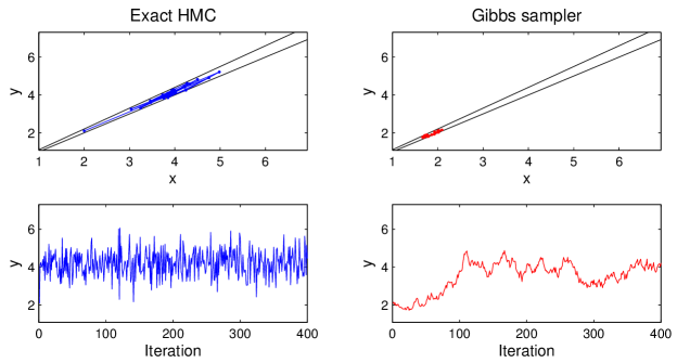
Figure 1: HMC vs Gibbs sampler. Comparison for a two-dimensional distribution with $\log p(x,y)\varpropto-\frac{1}{2}(x-4)^{2}-\frac{1}{2}(y-4)^{2}$, constrained to the wedge $x\leq y\leq 1.1x$ and $x,y\geq 0$. The initial point is $(x,y)=(2,2.1)$. Upper panels: first 20 iterations. Lower panels: Second coordinate of the first 400 iterations. In the HMC case we used $T=\pi/2$. The HMC sampler moves rapidly to oscillate around $y=4$, as desired, while the Gibbs sampler mixes relatively slowly.

2 The Sampling Algorithm

2.1 Linear Inequalities

Consider first sampling from

$$\log p(\textbf{X})=-\frac{1}{2}\textbf{X}\cdot\textbf{X}+const.$$ (2.1)

subject to

$$\textbf{F}_{j}\cdot\textbf{X}+g_{j}\geq 0\qquad j=1,\ldots,m\,.$$ (2.2)

Any quadratic form for $\log p(\textbf{X})$, as in (1.1), can be brought to the above canonical form by a linear change of variables. Let us denote the components of X and $\textbf{F}_{j}$ as

X $$= (x_{1},\ldots,x_{d})\,,$$ (2.3)

$$\textbf{F}_{j} = (f_{j}^{1},\ldots,f_{j}^{d})\,.$$ (2.4)

In order to apply the HMC method, we introduce momentum variables S,

$$\textbf{S}=(s^{1},\ldots,s^{d})\,,$$ (2.5)

and consider the Hamiltonian

$$H=\frac{1}{2}\textbf{X}\cdot\textbf{X}+\frac{1}{2}\textbf{S}\cdot\textbf{S}\,,$$ (2.6)

such that the joint distribution is $p(\textbf{X},\textbf{S})=\exp(-H)$. The equations of motion following from (2.6) are

$$\dot{x}_{i} = \frac{\partial H}{\partial s^{i}}=s^{i}$$ (2.7)

$$\dot{s}^{i} = -\frac{\partial H}{\partial x_{i}}=-x_{i}\qquad\qquad i=1,\ldots,d$$ (2.8)

which can be combined to

$$\ddot{x}_{i}=-x_{i}\,,$$ (2.9)

and have a solution

$$x_{i}(t) = a_{i}\sin(t)+b_{i}\cos(t)\,.$$ (2.10)

The constants $a_{i},b_{i}$ can be expressed in terms of the initial conditions as

$$a_{i} = \dot{x}_{i}(0)=s^{i}(0)$$ (2.11)

$$b_{i} = x_{i}(0)$$ (2.12)

The HMC algorithm proceeds by alternating between two steps. In the first step we sample S from $p(\textbf{S})={\cal N}(0,\mathbb{I}_{d})$. In the second step we use this S and the last value of X as initial conditions, and let the particle move during a time $T$, after which the position and momentum have values $\textbf{X}^{*}$ and $\textbf{S}^{*}$. The value $\textbf{X}^{*}$ belongs to a Markov chain with equilibrium distribution $p(\textbf{X})$. To see this, note that for a given $T$, the particle trajectory is deterministic once the momentum S is sampled, so the transition probability is

$$p(\textbf{X}^{*}|\textbf{X},T)=p(\textbf{S})\left|\partial\textbf{S}/\partial\textbf{X}^{*}\right|\,.$$ (2.13)

Two important properties of Hamiltonian dynamics are the conservation of energy

$$H(\textbf{X},\textbf{S})=H(\textbf{X}^{*},\textbf{S}^{*})$$ (2.14)

and the conservation of volume in phase space

$$d\textbf{S}^{*}d\textbf{X}^{*}=d\textbf{S}d\textbf{X}$$ (2.15)

which implies the equation

$$\left|\partial\textbf{S}/\partial\textbf{X}^{*}\right|=\left|\partial\textbf{S}^{*}/\partial\textbf{X}\right|\,.$$ (2.16)

From the above results the detailed balanced condition follows as

$$p(\textbf{X})p(\textbf{X}^{*}|\textbf{X},T) = p(\textbf{X})p(\textbf{S})\left|\partial\textbf{S}/\partial\textbf{X}^{*}\right|$$ (2.17)

$$= e^{-H(\textbf{X},\textbf{S})}\left|\partial\textbf{S}/\partial\textbf{X}^{*}\right|$$ (2.18)

$$= e^{-H(\textbf{X}^{*},-\textbf{S}^{*})}\left|\partial\textbf{S}^{*}/\partial\textbf{X}\right|$$ (2.19)

$$= p(\textbf{X}^{*})p(\textbf{X}|\textbf{X}^{*},T)$$ (2.20)

where we used the invariance of $H$ under $\textbf{S}\rightarrow-\textbf{S}$. We will discuss the appropriate choice for $T$ in Section 2.4.

The trajectory of the particle is given by (2.10) until it hits a wall, and this occurs whenever any of the inequalities (2.2) is saturated. To find the time at which this occurs, it is convenient to define

$$K_{j}(t) = \sum_{i=1}^{d}f_{j}^{i}x_{i}(t)+g_{j}\qquad j=1,\ldots,m\,.$$ (2.21)

$$= \sum_{i=1}^{d}f_{j}^{i}a_{i}\sin(t)+\sum_{i=1}^{d}f_{j}^{i}b_{i}\cos(t)+g_{j}$$ (2.22)

$$= u_{j}\cos(t+\varphi_{j})+g_{j}$$ (2.23)

where

$$u_{j} = \sqrt{(\sum_{i=1}^{d}f_{j}^{i}a_{i})^{2}+(\sum_{i=1}^{d}f_{j}^{i}b_{i})^{2}}\,,$$ (2.24)

$$\tan\varphi_{j} = -\frac{\sum_{i=1}^{d}f_{j}^{i}a_{i}}{\sum_{i=1}^{d}f_{j}^{i}b_{i}}\,.$$ (2.25)

Along the trajectory we have $K_{j}(t)\geq 0$ for all $j$ and a wall hit corresponds to $K_{j}(t)=0$, so from (2.23) it follows that the particle can only reach those walls satisfying $u_{j}>|g_{j}|$. Each one of those reachable walls has associated two times $t_{j}>0$ such that

$$K_{j}(t_{j})=0\,,$$ (2.26)

and the actual wall hit corresponds to the smallest of all these times. Suppose that the latter occurs for $j=h$. At the hitting point, the particle bounces off the wall and the trajectory continues with a reflected velocity. The latter can be obtained by noting that the vector $\textbf{F}_{h}$ is perpendicular to the reflecting plane. Let us decompose the velocity as

$$\dot{\textbf{X}}(t_{h})=\dot{\textbf{X}}_{\perp}(t_{h})+\alpha_{h}\textbf{F}_{h}\,,$$ (2.27)

where $\textbf{F}_{h}\cdot\dot{\textbf{X}}_{\perp}(t_{h})=0$ and

$$\alpha_{h} = \frac{\textbf{F}_{h}\cdot\dot{\textbf{X}}(t_{h})}{||\textbf{F}_{h}||^{2}}\,.$$ (2.28)

The reflected velocity, $\dot{\textbf{X}}_{R}(t_{h})$, is obtained by inverting the component perpendicular to the reflecting plane

$$\dot{\textbf{X}}_{R}(t_{h}) = \dot{\textbf{X}}_{\perp}(t_{h})-\alpha_{h}\textbf{F}_{h}\,,$$ (2.29)

$$= \dot{\textbf{X}}(t_{h})-2\alpha_{h}\textbf{F}_{h}\,.$$ (2.30)

It is easy to verify that this transformation leaves the Hamiltonian (2.6) invariant. Once the reflected velocity is computed, we use it as an initial condition in (2.11) to continue the particle trajectory.

If we prefer to keep the original distribution in the form (1.1), we should consider the Hamiltonian

$$H=\frac{1}{2}\textbf{X}^{T}\textbf{M}\textbf{X}-\textbf{r}^{T}\textbf{X}+\frac{1}{2}\textbf{S}^{T}\textbf{M}^{-1}\textbf{S}\,.$$ (2.31)

This election for the mass matrix leads to the simple solution

$$x_{i}(t) = \mu_{i}+a_{i}\sin(t)+b_{i}\cos(t)\,,$$ (2.32)

where

$$\mu_{i} = \sum_{j=1}^{d}M_{ij}^{-1}r_{j}\,,$$ (2.33)

$$a_{i} = \dot{x}_{i}(0)=\sum_{j=1}^{d}M_{ij}^{-1}s_{j}(0)\,,$$ (2.34)

$$b_{i} = x_{i}(0)-\mu_{i}\,.$$ (2.35)

Since the particle trajectory depends on $\dot{x}_{i}(0)$, we can start each iteration by sampling $\dot{x}_{i}(0)\sim{\cal N}(0,\textbf{M}^{-1})$, instead of sampling $s_{i}(0)\sim{\cal N}(0,\textbf{M})$ itself.

2.2 The runtime of the sampler

The runtime of each iteration has a contribution that scales linearly with $m$, the number constraints, since we have to compute the $m$ values $u_{j}$ at (2.24). But the dominant computational time goes to compute $\varphi_{j}$ and $t_{j}$, defined in (2.25) and (2.26), which only needs to be done when $u_{j}>|g_{j}|$. The average number of coordinates for which this condition occurs, as well as the number of times the particle hits the walls per iteration, varies according to the value of $T$ and the shape and location of the walls.

The sums in expressions (2.24) and (2.25) can be interpreted as matrix-vector multiplications, with cost $O(md)$ for general constraint matrices $\textbf{F}=(\textbf{F}_{1}^{T}\textbf{F}_{2}^{T}\ldots\textbf{F}_{m}^{T})^{T}$. Note that these matrix-vector multiplications are highly parallelizable. In addition, in many cases there may be some special structure that can be exploited to speed computation further; for example, if F can be expressed as a sparse matrix in a convenient basis, this cost can be reduced to $O(d)$.

Also, in both frames (2.6) and (2.31) we must act, for each sample, with a matrix $R^{-1}$, where $\textbf{M}=R^{T}R$. Equivalently, we must multiply by $Z^{T}$, where $\textbf{M}^{-1}=\Sigma=Z^{T}Z$. In the frame (2.6) this is needed because the samples must be mapped back to the original frame (1.1) as

$$\textbf{X}\rightarrow R^{-1}\textbf{X}+\textbf{M}^{-1}\textbf{r}\,,$$ (2.36)

and in the frame (2.31) the action of $R^{-1}$ is needed in order to sample the initial velocity from ${\cal N}(0,\textbf{M}^{-1})$ at each iteration. The action of $R^{-1}$ takes $O(d^{2})$ generally, but in some cases the matrix M or its inverse have a special structure that allows us to accelerate this operation. This is the case in the four example applications we present in Section 3.

Regarding which of the two frames (2.6) and (2.31) is preferred, this depends on the nature of the constraints, since the latter change when we transform the quadratic form for $\log p(\textbf{X})$ in (1.1) to the form (2.1). For example, a sparse set of constraints F in the original frame leads to a fast evaluation of (2.24) and (2.25), but the wall geometry in the transformed frame may lead to a smaller number of wall hits and therefore shorter runtime.

2.3 Quadratic and Higher Order Inequalities

The sampling algorithm can be extended in principle to polynomial constraints of the form

$$Q_{j}(\textbf{X})\geq 0\qquad j=1,\ldots,m\,.$$ (2.37)

Evaluating $Q_{j}(\textbf{X})$ at the solution (2.10) leads to a polynomial in $\sin(t)$ and $\cos(t)$, whose zeros must be found in order to find the hitting times. When a wall is hit, we reflect the velocity by inverting the sign of the component perpendicular to the wall, given by the gradient ${\bf\nabla}Q_{j}(\textbf{X})$. This vector plays a role similar to $\textbf{F}_{j}$ in (2.27)-(2.30). Of course, for general polynomials $Q_{j}(\textbf{X})$ computing the hitting times might be numerically challenging.

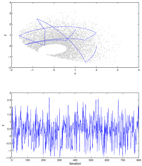
Figure 2: Truncation by quadratic inequalities. Above: 6000 samples of a two-dimensional canonical normal distribution, constrained by the quadratic inequalities (2.54) -(2.55). The piecewise elliptic curve shows the trajectory of the particle in the first iterations, with starting point $(x,y)=(2,0)$. Below: first $800$ iterations of the vertical coordinate. For the algebraic solution of (2.48), we used the C++ code from the DynamO package (Bannerman et al., 2011).

One family of solvable constraints involves quadratic inequalities of the form

$$Q_{j}(\textbf{X})=\textbf{X}^{T}\textbf{A}_{j}\textbf{X}+\textbf{X}\cdot\textbf{B}_{j}+C_{j}\geq 0\qquad j=1,\ldots,m\,,$$ (2.38)

where $\textbf{A}_{j}\in\mathbb{R}^{d,d},\,\textbf{B}_{j}\in\mathbb{R}^{d},\,C_{j}\in\mathbb{R}$. For statistics applications where these constraints are important, see e.g. Ellis and Maitra (2007). Inserting (2.10) in the equality for (2.38) leads, for each $j$, to the following equation for the hitting time:

$$q_{1}\cos^{2}(t)+q_{2}\cos(t)+q_{3}=-\sin(t)(q_{4}\cos(t)+q_{5})\,,$$ (2.39)

with

$$q_{1} = \sum_{i,k}A^{ik}b_{i}b_{k}-\sum_{ik}A^{ik}a_{i}a_{k}\,,$$ (2.40)

$$q_{2} = \sum_{i}B^{i}b_{i}\,,$$ (2.41)

$$q_{3} = C+\sum_{ik}A^{ik}a_{i}a_{k}\,,$$ (2.42)

$$q_{4} = 2\sum_{i,k}A^{ik}a_{i}b_{k}\,,$$ (2.43)

$$q_{5} = \sum_{i}B^{i}a_{i}\,,$$ (2.44)

and we omitted the $j$ dependence to simplify the notation. If the ellipse in (2.38) is centered at the origin, we have $\textbf{B}_{j}=q_{2}=q_{5}=0$, and equation (2.39) simplifies to

$$q_{1}+2q_{3}+u\sin(2t+\varphi)=0$$ (2.45)

where

$$u^{2} = q_{1}^{2}+q_{4}^{2}\,,$$ (2.46)

$$\tan\varphi = \frac{q_{1}}{q_{4}}\,,$$ (2.47)

and the hit time can be found from (2.45) as in the linear case. In the general $\textbf{B}_{j}\neq 0$ case, the square of (2.39) gives the quartic equation

$$r_{4}\cos^{4}(t)+r_{3}\cos^{3}(t)+r_{2}\cos^{2}(t)+r_{1}\cos(t)+r_{0}=0\,,$$ (2.48)

where

$$r_{4} = q_{1}^{2}+q_{4}^{2}\,,$$ (2.49)

$$r_{3} = 2q_{1}q_{2}+2q_{4}q_{5}\,,$$ (2.50)

$$r_{2} = q_{2}^{2}+2q_{1}q_{3}+q_{5}^{2}-q_{4}^{2}\,,$$ (2.51)

$$r_{1} = 2q_{2}q_{3}-2q_{4}q_{5}\,,$$ (2.52)

$$r_{0} = q_{3}^{2}-q_{5}^{2}\,.$$ (2.53)

Equation (2.48) can be solved exactly for $cos(t)$ using standard algebraic methods (Herbison-Evans, 1994). A wall hit corresponds, among all the constraints $j$, to the solution for $\cos(t)$ with smallest $t>0$ and $|\cos(t)|\leq 1$, which also solves (2.39). As an example, Figure 2 shows samples from a two-dimensional canonical normal distribution, constrained by

$$\frac{(x-4)^{2}}{32}+\frac{(y-1)^{2}}{8} \leq 1\,,$$ (2.54)

$$4x^{2}+8y^{2}-2xy+5y \geq 1\,.$$ (2.55)

Equipped with the results for linear and quadratic constraints, we can also find the hitting times for constraints of the form

$$Q(\textbf{X})=\prod_{j}Q_{j}(\textbf{X})\geq 0$$ (2.56)

where each $Q_{j}(\textbf{X})$ is a linear or a quadratic function. Each factor defines an equation as (2.26) or (2.48), and the hitting time is the smallest at which any factor becomes zero. For other polynomials, one has to resort to numerical methods to find the hitting times.

2.4 Travel time and efficiency

The value of $T$ should be chosen to make the sampling as efficient as possible. This is not easy because the path of the particle will be determined by the wall bounces, so it is difficult to compute in advance. A safe strategy is to choose a value of $T$ that makes the sampling efficient at least for those trajectories with no wall hits. The efficiency can be quantified via the Effective Sample Factor (ESF) and Effective Sample Size (ESS) (Liu, 2008). Let us call the samples $\textbf{X}^{(p)}$. The variance in the estimation of the expected value of a function $h(\textbf{X})$ using $m$ samples is

$$var\left(\frac{h(\textbf{X}^{(1)})+\cdots+h(\textbf{X}^{(m)})}{m}\right)=\frac{var(h(\textbf{X}))}{m}\left[1+\sum_{j=1}^{m-1}2\left(1-\frac{j}{m}\right)\rho_{j}\right]$$ (2.57)

with $\rho_{j}$ the autocorrelation function (ACF),

$$\rho_{j} = corr[h(\textbf{X}^{(1)}),h(\textbf{X}^{(1+j)})]\,.$$ (2.58)

The ESF and ESS are defined as

ESF $$= \left[1+\sum_{j=1}^{m-1}2\left(1-\frac{j}{m}\right)\rho_{j}\right]^{-1}\,,$$ (2.59)

ESS $$= m\times\textrm{ESF }\,,$$ (2.60)

and a sampling scheme is more efficient when its ESF is higher, because that leads to a lower variance in (2.57).

For concreteness, let us consider the estimation of the mean of a coordinate $x_{i}$ in the frame in which the Hamiltonian is given by (2.6). In the absence of wall hits, from (2.10)-(2.11) it follows that successive samples are given by

$$x^{(p+1)}_{i}=x_{i}^{(p)}\cos(T)+s_{i}^{(p)}\sin(T)\,.$$ (2.61)

Assuming that the momenta samples are i.i.d., i.e.,

$$\langle s_{i}^{(p)}s_{i}^{(q)}\rangle=\delta_{pq}\,,$$ (2.62)

it is easy to see that the ACF is given by

$$\rho_{j}=\langle x_{i}^{(1)}x_{i}^{(j+1)}\rangle=\cos^{j}(T)\,.$$ (2.63)

In principle we could plug this expression into (2.59) and find the value of $T$ that maximizes the ESF. In particular, when $\cos(T)<0$, there are values of $T$ which lead to a super-efficient sampler with ESF $>1$, so that the variance (2.57) is smaller than using i.i.d. samples (i.e., with $\rho_{j}=0$). This is similar to the antithetic variates method to reduce the variance of Monte Carlo estimates (Hammersley and Morton, 1956).

	Avg. CPU Time		$y$
$\textrm{HMC}_{T=\pi/2}$	3.78 secs	ESF	2.7 (1.18/5.11)
		ESS/CPU	5,802 (2,507/10,096)
$\textrm{HMC}_{T=\pi/10}$	1.38 secs	ESF	0.052 (0.033/0.094)
		ESS/CPU	301 (191/547)
Gibbs	0.57 secs	ESF	0.017 (0.011/0.032)
		ESS/CPU	237 (154/456)

Table 1: HMC vs Gibbs sampler. Comparison of efficiency criteria for 30 runs of three samplers in the example of Figure 1. For the definition of ESF and ESS, see Section 2.4. ESS/CPU is the Effective Sample Size in units of the CPU runtime. A sampler is more efficient for higher ESF and ESS/CPU. In each run, we used 8,000 samples, after discarding 2,000 samples as burn-in. The CPU time for each run is random, but its variability across runs is negligible due to the large number of samples. For ESF and ESS/CPU, we show median (first/third quartiles). For the Gibbs sampler, we used the algorithm of (Damien and Walker, 2001). The runtime for HMC is relatively high due to the many reflections of the particle against the walls. Note that the efficiency of the HMC sampler depends strongly on the value of the travel time $T$.

In practice, we have found that the above strategy is not very useful. The assumption (2.62) holds only approximately for standard generators of random variables, and this leads to very unstable values for the ESF for any value of $T$. A safe choice is to use $T=\pi/2$, which leads to

$$x^{(p+1)}_{i}=s_{i}^{(p)}\,,$$ (2.64)

so our sampling of the space X, for trajectories with no wall hits, will be as efficient as our method to sample the momenta S. Since the i.i.d. assumption holds approximately, this leads to values of ESF that bounce around $1$. The ESF in a general case will also depend on the shape and location of the constraint walls. But we have found that the super-efficient case ESF $>1$ is not uncommon, although as mentioned, the actual value of the ESF is quite unstable. Table 1 illustrates the big difference in the efficiency of the HMC sampler for $T=\pi/2$ and $T=\pi/10$ in the two-dimensional example of Figure 1. A similar reasoning suggests the use of $T=\pi/2$ also when working in the frame in which the Hamiltonian is given by (2.31). In the next two Sections we adopted $T=\pi/2$, and we rotated the coordinates to a canonical frame with Hamiltonian (2.6).

In Tables 1 and 2 we compare the efficiency of our HMC method to the Gibbs sampler. To implement the latter efficiently we made two choices. Firstly, we rotated the coordinates to a canonical frame in which the unconstrained Gaussian has unit covariance. This transformation often makes the Gibbs sampler mix faster (Rodriguez-Yam et al., 2004). For the Gibbs sampler itself, we used the slice sampling version of (Damien and Walker, 2001). This algorithm augments by one the number of variables, but turns the conditional distributions of the coordinates of interest into uniform distributions. The latter are much faster to sample than the truncated one-dimensional Gaussians one gets otherwise. We checked that the efficiency of the algorithm of (Damien and Walker, 2001), measured in units of ESS/CPU time, is much higher than that of the Gibbs sampler based on direct sampling from the one-dimensional truncated normal using inverse cdf or rejection sampling.

3 Examples

In this Section we present four example applications of our algorithm. In the first example, we present a detailed efficiency comparison between the HMC and the Gibbs samplers. As mentioned in Section 2.2, in both frames (2.6) and (2.31), for each sample of the HMC we must act with a matrix $R^{-1}$, where $\textbf{M}=R^{T}R$, or multiply by $Z^{T}$, where $\textbf{M}^{-1}=\Sigma=Z^{T}Z$. In all our examples, we show how some special structure of M or $\Sigma$ allows us to accelerate these operations.

3.1 Probit and Tobit Models

The Probit model is a popular discriminative probabilistic model for binary classification with continuous inputs (Albert and Chib, 1993). The conditional probabilities for the binary labels $y=\pm 1$ are given by

$$p(y=-1|\textbf{z},\boldsymbol{\beta}) = \Phi(\textbf{z}\cdot\boldsymbol{\beta})=\frac{1}{\sqrt{2\pi}}\int_{-\infty}^{\textbf{z}\cdot\boldsymbol{\beta}}\!\!\!\!\!\!dw\,e^{-\frac{w^{2}}{2}}$$ (3.1)

$$= \frac{1}{\sqrt{2\pi}}\int_{-\infty}^{0}\!\!\!\!\!\!dw\,e^{-\frac{(w+\textbf{z}\cdot\boldsymbol{\beta})^{2}}{2}}$$ (3.2)

$$p(y=+1|\textbf{z},\boldsymbol{\beta}) = 1-\Phi(\textbf{z}\cdot\boldsymbol{\beta})$$ (3.3)

$$= \frac{1}{\sqrt{2\pi}}\int^{+\infty}_{0}\!\!\!\!\!\!dw\,e^{-\frac{(w+\textbf{z}\cdot\boldsymbol{\beta})^{2}}{2}}$$ (3.4)

where $\textbf{z}\in\mathbb{R}^{p}$ is a vector of regressors and $\boldsymbol{\beta}\in\mathbb{R}^{p}$ are the parameters of the model. Given $N$ pairs of labels and regressors

$$\textbf{Y}=(y_{1},\ldots,y_{N})\,,$$ (3.5)

$$\textbf{Z}=(\textbf{z}_{1},\ldots,\textbf{z}_{N})\,,$$ (3.6)

the posterior distribution of the parameters $\boldsymbol{\beta}$ is

$$p(\boldsymbol{\beta}|\textbf{Y},\textbf{Z}) \varpropto p(\boldsymbol{\beta})\prod_{i=1}^{N}p(y_{i}|\textbf{z}_{i},\boldsymbol{\beta})$$ (3.7)

$$\varpropto p(\boldsymbol{\beta})\int_{y_{i}w_{i}\geq 0}\!\!\!\!\!\!\!\!\!\!\!\!dw_{1}\ldots dw_{N}\,\,e^{-\frac{1}{2}\sum_{i=1}^{N}(w_{i}+\textbf{z}_{i}\cdot\boldsymbol{\beta})^{2}}\qquad i=1,\ldots,N,$$ (3.8)

where $p(\boldsymbol{\beta})$ is the prior distribution.

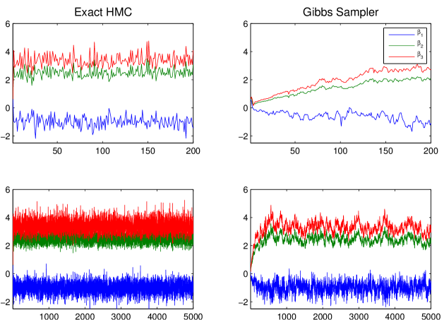
Figure 3: Bayesian Probit model. First 200 and 5000 samples from the posterior (3.8) of a model with $p=3$. $N=800$ pairs $(y_{i},z_{i})$ were generated with $\beta_{1}=-9,\beta_{2}=20,\beta_{3}=27$ and we assumed a Gaussian prior with zero mean and $\sigma^{2}=1$. Note that the means of the sampled values are different from the values used to generate the data, due to the zero-mean prior. Left: Exact HMC sampler. Right: Gibbs sampler, with whitened covariance to improve mixing (Rodriguez-Yam et al., 2004).

The likelihood $p(y_{i}|\textbf{z}_{i},\boldsymbol{\beta})$ corresponds to a model

$$y_{i} = sign(w_{i})$$ (3.9)

$$w_{i} = -\textbf{z}_{i}\cdot\boldsymbol{\beta}+\varepsilon_{i}$$ (3.10)

$$\varepsilon_{i} \sim {\cal N}(0,1)$$ (3.11)

in which only the sign of $w_{i}$ is observed, but not its value. Assuming a Gaussian prior with zero mean and covariance $\sigma^{2}\mathbb{I}_{p}$, expression (3.8) is the marginal distribution of a multivariate Gaussian on $(\boldsymbol{\beta},w_{1},\ldots w_{N}),$ truncated to $y_{i}w_{i}\geq 0$ for $i=1,\ldots,N$. The untruncated Gaussian has zero mean and precision matrix

M $$= \begin{pmatrix}M_{\boldsymbol{\beta}\,\boldsymbol{\beta}}&M_{\boldsymbol{\beta}\,w}\\ M_{w\,\boldsymbol{\beta}}&M_{ww}\end{pmatrix}\qquad\in\mathbb{R}^{p+N,p+N}$$ (3.12)

$$= \begin{pmatrix}\sigma^{-2}\mathbb{I}_{p}+BB^{T}&B\\ B^{T}&\mathbb{I}_{N}\end{pmatrix}$$ (3.13)

where

$$B^{T} = \begin{pmatrix}\textbf{z}_{1}\\ \vdots\\ \textbf{z}_{N}\end{pmatrix}\qquad\in\mathbb{R}^{N,p}$$ (3.14)

We can sample from the posterior in (3.8) by sampling from the truncated Gaussian for $(\boldsymbol{\beta},w_{1},\ldots w_{N})$ and keeping only the $\boldsymbol{\beta}$ values. It is easy to show that without the term $\sigma^{-2}\mathbb{I}_{p}$ in (3.13), coming from the prior $p(\boldsymbol{\beta}),$ the precision matrix would have $p$ null directions and our method would not be applicable, since we assume the precision matrix to be positive definite. Note that the dimension of the TMG grows linearly with the number $N$ of data points.

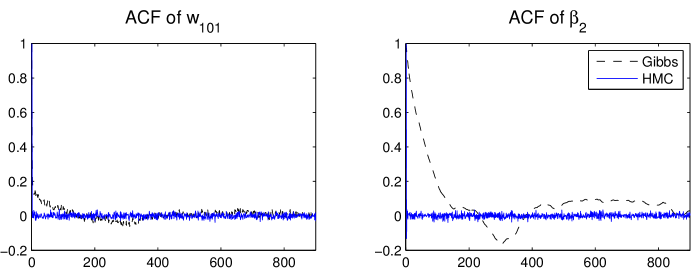
Figure 4: Autocorrelation functions. Autocorrelation functions (ACFs) for the first 900 lags of two of the 803 variables sampled in the Probit example. See Table 2 for a comparison of efficiency measures of these two variables between the two samplers.

The structure of (3.13) leads to a simple form for the untruncated covariance $\Sigma=\textbf{M}^{-1}$,

$$\textbf{M}^{-1} = \begin{pmatrix}\mathbb{I}_{p}&0\\ -B^{T}&\mathbb{I}_{N}\end{pmatrix}\begin{pmatrix}\sigma^{2}\mathbb{I}_{p}&0\\ 0&\mathbb{I}_{N}\end{pmatrix}\begin{pmatrix}\mathbb{I}_{p}&-B\\ 0&\mathbb{I}_{N}\end{pmatrix}$$ (3.15)

$$= Z^{T}Z$$ (3.16)

where

$$Z^{T}=\begin{pmatrix}\mathbb{I}_{p}&0\\ -B^{T}&\mathbb{I}_{N}\end{pmatrix}\begin{pmatrix}\sigma\mathbb{I}_{p}&0\\ 0&\mathbb{I}_{N}\end{pmatrix}\,,$$ (3.17)

and this form is such that acting with $Z^{T}$ takes $O(N)$ time, instead of $O(N^{2})$ .

As an illustration, Figure 3 shows the values of $\boldsymbol{\beta}$, sampled using Gibbs and exact HMC, from the posterior of a model with $p=3$ where $N=800$ data points were generated. We used $z^{1}_{i}=1$, $z^{2}_{i}\sim Unif[-5,+5]$ and $z^{3}_{i}\sim{\cal N}(-4,\sigma=4)$. The values of $y_{i}$ were generated with $\beta_{1}=-9,\beta_{2}=20,\beta_{3}=27$ and we assumed a Gaussian prior with $\sigma^{2}=1$. Note that the means of the sampled $\beta_{i}$’s are different from the $\beta_{i}$’s used to generate the data, due to the prior which pulls the $\beta_{i}$’s towards zero.

A more quantitative comparison between the HMC and the Gibbs samplers is presented in Figure 4, which compares the autocorrelation functions (ACFs) for two of the variables of the Probit model, and in Table 2, which compares, for the same variables, the Effective Sample Factors (ESFs) and the Effective Sample Size (ESS) normalized by CPU time. For the latter, we see a remarkable difference of two to three orders of magnitude between the two samplers.

	Avg. CPU time		$w_{101}$	$\beta_{2}$
HMC	$235.5$ secs.	ESF	1.96 (1.28/7.03)	2.65 (1.28/3.69)
		ESS/CPU	49.9 (32.6/178.6)	67.69 (32.6/92.84)
Gibbs	$651.7$ secs.	ESF	0.037 (0.027/0.054)	0.0051 (0.0036/0.0068)
		ESS/CPU	0.34 (0.22/0.50)	0.047 (0.033/0.063)

Table 2: Efficiency of HMC vs. Gibbs in the Probit example. The results summarize 10 runs of each sampler, and correspond to the means of the variables $w_{101}$ and $\beta_{2}$ from the $803$-dimensional Probit example. The autocorrelation functions of these variables are shown in Figure 4. In each run we used 6,000 samples, after discarding 2,000 samples as burn-in. Again, the CPU time for each run is random, but its variability across runs is negligible due to the large number of samples. For ESF and ESS/CPU, we show median (first/third quartiles). ESS/CPU is the Effective Sample Size in units of the CPU runtime. For Gibbs we used the algorithm of (Damien and Walker, 2001). Note that the efficiency criteria are fairly variable across runs, but the HMC ESS/CPU is consistently two to three orders of magnitude bigger than Gibbs. The Gibbs sampler shows a big difference in the efficiency between the two variables (cf. their ACFs in Figure 4), while this difference is minor in the HMC case. The HMC runtime can be reduced further by parallelizing the computation of the travel times to hit each wall.

A model related to the Probit is the Tobit model for censored data (Tobin, 1958), which is a linear regression model where negative values are not observed:

$$y_{i}=\left\{\begin{array}[]{ll}y_{i}^{*}&\textrm{for}\,y_{i}^{*}>0\,,\\ 0&\textrm{for}\,y_{i}^{*}\leq 0\,,\end{array}\right.$$ (3.20)

where

$$y_{i}^{*}=\textbf{z}_{i}\cdot\boldsymbol{\beta}+\varepsilon_{i}\,,\qquad\varepsilon_{i}\sim{\cal N}(0,\sigma).$$ (3.21)

The likelihood of a pair $(y_{i},\textbf{z}_{i})$ is

$$p(y_{i}|\textbf{z}_{i},\boldsymbol{\beta},\sigma)=\left\{\begin{array}[]{ll}\frac{e^{-\frac{(y_{i}-\textbf{z}_{i}\cdot\boldsymbol{\beta})^{2}}{2\sigma^{2}}}}{\sqrt{2\pi\sigma^{2}}}&\textrm{for}\,y_{i}>0\,,\\ \frac{1}{\sqrt{2\pi\sigma^{2}}}\int_{-\infty}^{0}dw_{i}e^{-\frac{(w_{i}-\textbf{z}_{i}\cdot\boldsymbol{\beta})^{2}}{2\sigma^{2}}}&\textrm{for}\,y_{i}=0\,,\end{array}\right.$$ (3.24)

and the posterior probability for $\boldsymbol{\beta}$ is

$$p(\boldsymbol{\beta}|\textbf{Y},\textbf{Z},\sigma) \varpropto p(\boldsymbol{\beta}|\sigma)\,\prod_{i=1}^{N}p(y_{i}|\textbf{z}_{i},\boldsymbol{\beta},\sigma)$$ (3.25)

$$\varpropto p(\boldsymbol{\beta}|\sigma)\,\prod_{i,y_{i}>0}e^{-\frac{(y_{i}-\textbf{z}_{i}\cdot\boldsymbol{\beta})^{2}}{2\sigma^{2}}}\prod_{i,y_{i}=0}\int_{-\infty}^{0}\!\!dw_{i}\,\,e^{-\frac{(w_{i}-\textbf{z}_{i}\cdot\boldsymbol{\beta})^{2}}{2\sigma^{2}}}$$ (3.26)

As in (3.8), this can be treated as a marginal distribution over the variables $w_{i}$, with the joint distribution for $(\boldsymbol{\beta},w_{i})$ a truncated multivariate Gaussian.

One can similarly consider multivariate Probit (Ashford and Sowden, 1970) and Tobit models. For the former, the Bayesian approach has been shown to be superior to Maximum Likelihood (Geweke et al., 1994).

3.2 Sample paths in a Brownian bridge

A family of cases where a simple special structure for M arises are linear-Gaussian state-space models with constraints on the hidden variables. For concreteness, we will study the case of the Brownian bridge. Consider the following discrete stochastic process

$$V_{t} = V_{t-1}+\varepsilon_{t}\qquad\varepsilon_{t}\sim{\cal N}(0,\sigma^{2})\qquad t=1,\ldots,T$$ (3.27)

$$V_{0} = L\leq H$$ (3.28)

$$V_{t} < V_{T}\quad\quad\quad\quad\quad\textrm{for}\,\,\,\,\,t<T$$ (3.29)

$$V_{T} = H$$ (3.30)

The starting point $V_{0}=L$ is fixed and the number of steps $T$ until the first hit of $H$ is a random variable. This process is called the Brownian bridge and has applications, among others, in finance (see e.g. (Glasserman, 2003) ) and in neuroscience, where it corresponds to a stochastic integrate-and-fire model (see e.g. (Paninski et al., 2004)). Given $T$, we are interested in samples from the $(T-1)$-dimensional space of possible paths. The log-density is given by

$$\log p(V_{1},\ldots,V_{T-1}|V_{0},V_{T},\sigma^{2}) = -\frac{1}{2\sigma^{2}}\sum_{t=1}^{T}(V_{t}-V_{t-1})^{2}+const.$$ (3.31)

$$= -\frac{1}{2}V^{T}\textbf{M}V+\textbf{r}^{T}V+const.$$ (3.32)

with

$$V_{t}<H\qquad\qquad\textrm{for}\qquad t=1,\ldots T-1,$$ (3.33)

and we defined

$$V^{T} = (V_{1},\ldots,V_{T-1})\qquad\in\mathbb{R}^{T-1}$$ (3.34)

M $$= \sigma^{-2}\begin{pmatrix}2&-1\\ -1&2&-1\\ &&.&&&\\ &&&.&&\\ &&-1&2&-1&\\ &&&-1&-2&-1\\ &&&&-1&2\end{pmatrix}\quad\in\mathbb{R}^{T-1\times T-1}$$ (3.35)

$$\textbf{r}^{T} = (\sigma^{-2}V_{0},0,\ldots,0,\sigma^{-2}V_{T})\qquad\in\mathbb{R}^{T-1}$$ (3.36)

This is a $(T-1)$-dimensional TMG with tridiagonal precision matrix M. Therefore, in the Cholesky decomposition $\textbf{M}=R^{T}R$, $R$ is bidiagonal and the action of $R^{-1}$ takes $O(T)$ time instead of $O(T^{2})$. Figure 5 shows samples from this distribution.

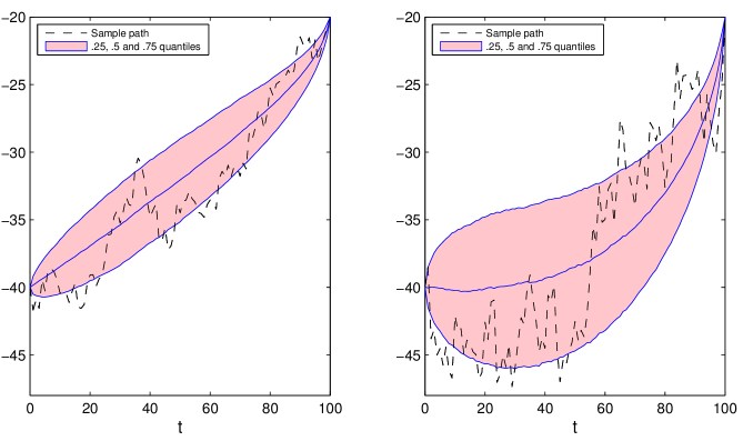
Figure 5: Sample paths in a Brownian bridge. Each figure shows one sample path and the median and $.25$ and $.75$ quantiles at each $t$ from $15,000$ sample paths (after 500 burn-in paths) of a Brownian bridge model with $L=-40,$ $H=-20$ and $T=100$. Left: low noise, $\sigma^{2}=1$. Right: high noise, $\sigma^{2}=5$.

3.3 Bayesian splines for positive functions

Suppose we have noisy samples $(y_{i},x_{i}),\,i=1\ldots N,$ from an unknown smooth positive function $f(x)>0,$ with $x\in[0,h]$. We can estimate $f(x)$ using cubic splines with knots at the $x_{i}$’s, plus $0$ and $h$ (Green and Silverman, 1994). The dimension of the vector space of cubic splines with $N$ inner knots is $N+4$. Our model is thus

$$y_{i}=\sum_{s=1}^{N+4}a_{s}\phi_{s}(x_{i})+\varepsilon_{i}\quad\varepsilon_{i}\sim{\cal N}(0,\sigma)\qquad i=1\ldots N\,,$$ (3.37)

where the functions $\phi_{s}(x)$ are a spline basis. Suppose we are interested in the value of $f(x)$ at the points $x=z_{j}$ with $j=1\ldots m$. To enforce $f(x)>0$ at those points, we impose the constraints

$$\boldsymbol{\phi}(z_{j})\cdot\textbf{a}\geq 0\,,\qquad j=1\ldots m\,,$$ (3.38)

where

$$\boldsymbol{\phi}(x) = (\phi_{1}(x),\ldots,\phi_{N+4}(x))\,,$$ (3.39)

a $$= (a_{1},\ldots,a_{N+4})\,.$$ (3.40)

To obtain a sparse constraint matrix, it is convenient to use the B-spline basis, in which only four elements in the vector $\boldsymbol{\phi}(z_{j})$ are non-zero for any $j$ (see, e.g. (De Boor, 2001) for details). In a Bayesian approach, we are interested in sampling from the posterior distribution

$$p(\textbf{a},\sigma^{2}|\textbf{Y},\textbf{X},\lambda)\varpropto p(\textbf{Y}|\textbf{X},\textbf{a},\sigma^{2})p(\textbf{a}|\lambda,\sigma^{2})p(\sigma^{2})\,,$$ (3.41)

where we defined

Y $$= (y_{1},\ldots,y_{N})\,,$$ (3.42)

X $$= (x_{1},\ldots,x_{N})\,.$$ (3.43)

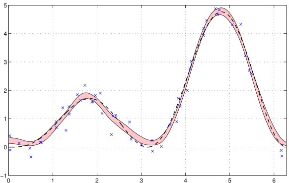
Figure 6: Bayesian splines for positive functions. The crosses show $50$ samples from $y_{i}=x_{i}\,\sin^{2}(x_{i})+\varepsilon_{i}$, where $\varepsilon_{i}\sim{\cal N}(0,\sigma^{2})$ with $\sigma^{2}=.09$. The values of $x_{i}$ were sampled uniformly from $[0,2\pi]$. The curve $f(x)=x\,\sin^{2}(x)$ is shown as a dashed line. The shaded band shows the splines built with coefficients from the $.25$ and $.75$ quantiles of samples from the posterior distribution of a in (3.41). We used a Jeffreys prior for $\sigma^{2}$ (Jeffreys, 1946) and imposed the positivity constraints (3.38) at $100$ points spread uniformly in $[0,2\pi]$. The smoothness parameter $\lambda$ was estimated as $\hat{\lambda}=0.0067$ by maximizing the marginal likelihood (empirical Bayes criterion), using a Monte Carlo EM algorithm. The mean of the samples of $\sigma^{2}$ was $\hat{\sigma^{2}}=0.091$. The spline computations were performed with the “fda” MATLAB package (Ramsay et al., 2009).

The likelihood is

$$p(\textbf{Y}|\textbf{X},\textbf{a},\sigma^{2})=\frac{1}{({2\pi\sigma^{2}})^{N/2}}\exp\left(-\frac{1}{2\sigma^{2}}\sum_{i=1}^{N}(y_{i}-\textbf{a}\cdot\boldsymbol{\phi}(x_{i}))^{2}\right)\,,$$ (3.44)

and for the prior on a we consider

$$p(\textbf{a}|\lambda,\sigma^{2}) \varpropto \left(\frac{\lambda}{\sigma^{2}}\right)^{\frac{N+4}{2}}\exp\left(-\frac{\lambda}{2\sigma^{2}}\int_{0}^{h}dx\,\left(\textbf{a}\cdot\boldsymbol{\phi}^{\prime\prime}(x)\right)^{2}\right)\,,$$ (3.45)

$$\varpropto \left(\frac{\lambda}{\sigma^{2}}\right)^{\frac{N+4}{2}}\exp\left(-\frac{\lambda}{2\sigma^{2}}\,\textbf{a}^{T}\textbf{K}\textbf{a}\right)\,,$$ (3.46)

where $\textbf{K}\in\mathbb{R}^{N+4,N+4}$ has entries

$$K_{sr}=\int_{0}^{h}dx\,\phi^{\prime\prime}_{s}(x)\phi^{\prime\prime}_{r}(x)\,.$$ (3.47)

The prior (3.45)-(3.46) is standard in the spline literature and imposes a $\lambda$-dependent penalty on the roughness of the estimated polynomial, with a bigger $\lambda$ corresponding to a smoother solution. This penalty helps to avoid overfitting the data (Green and Silverman, 1994).

We can Gibbs sample from the posterior (3.41) by alternating between the conditional distributions of $\sigma^{2}$ and a. The latter is a TMG with

$$\log p(\textbf{a}|\sigma^{2},\textbf{X},\textbf{Y},\lambda)\varpropto-\frac{1}{2\sigma^{2}}\,\textbf{a}^{T}(\textbf{M}+\lambda\textbf{K})\textbf{a}+\frac{1}{\sigma^{2}}\textbf{a}^{T}\cdot\textbf{r}\,,\qquad s=1\ldots N+4\,,$$ (3.48)

constrained by (3.38), and we defined

M $$= \sum_{i=1}^{N}\boldsymbol{\phi}(x_{i})\boldsymbol{\phi}(x_{i})^{T}\qquad\in\mathbb{R}^{N+4,N+4}\,,$$ (3.49)

r $$= \sum_{i=1}^{N}y_{i}\boldsymbol{\phi}(x_{i})\qquad\in\mathbb{R}^{N+4}\,.$$ (3.50)

In the B-spline basis, the matrices M and K in (3.48) have a banded form (De Boor, 2001). As in Example 3.2 above, this allows us to speed up the runtime from $O(N^{2})$ to $O(N)$ for each sample.

Figure 6 shows an example for the function $f(x)=x\,\sin^{2}(x)$, with $N=50$ points sampled as

$$y_{i}=x_{i}\,\sin^{2}(x_{i})+\varepsilon_{i}\quad\varepsilon_{i}\sim{\cal N}(0,\sigma)\qquad\sigma^{2}=.09\,,$$ (3.51)

and with the $x_{i}$ sampled uniformly from $[0,2\pi]$.

3.4 Bayesian reconstruction of quantized stationary Gaussian processes

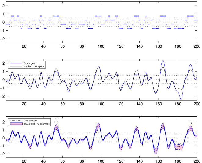
Figure 7: Bayesian reconstruction of quantized functions. Upper panel: a function quantized at $N=200$ points, taking four possible values. Middle panel: true function and median of the posterior samples. Lower panel: one posterior sample and median and $.25$ and $.75$ quantiles of the posterior samples. The three dotted lines, at $y=0,\,\pm.5$, separate the four quantization regions. We used $5,000$ samples, after discarding $500$ as burn-in. The $N=200$ values of the true function were sampled from a Gaussian process with kernel given by (3.58) with $\sigma^{2}=0.6,\,\eta^{2}=0.2$. Using the translation invariance of this kernel, the covariance matrix of the Gaussian can be embedded into a circulant matrix, and this allows to sample the initial velocity at every iteration of the HMC sampler in $O(N\log N)$ time instead of $O(N^{2})$.

Suppose that we are given $N$ values of a function $f(x_{i})\,,\,i=1,\ldots,N$, that takes discrete values in a set $\{q_{k}\}\,,\,k=1,\ldots,K$. We assume that this is a quantized projection of a sample $y(x_{i})$ from a stationary Gaussian process with a known translation-invariant covariance kernel of the form

$$(M^{-1})_{ij}=\Sigma_{ij}=K(|x_{i}-x_{j}|)\,,$$ (3.52)

and the quantization follows a known rule of the form

$$f(x_{i})=q_{k}\qquad\textrm{if}\qquad z_{k}\leq y(x_{i})<z_{k+1}\,.$$ (3.53)

We are interested in sampling the posterior distribution

$$p(y(x_{1}),\ldots,y(x_{N})|f(x_{1}),\ldots,f(x_{N}))\,,$$ (3.54)

which is a Gaussian with covariance (3.52), truncated by the quantization rules (3.53). In this case, we can exploit the Toeplitz form of the $N$-by-$N$-covariance matrix $\Sigma_{ij}$ to reduce the runtime of the HMC sampler. The idea is to embed $\Sigma$ into a circulant matrix as (see e.g., (Chu and George, 1999))

$$C = \begin{pmatrix}\Sigma_{11}&\Sigma_{12}&.&.&\Sigma_{1(N-1)}&\Sigma_{1N}&\Sigma_{1(N-1)}&.&.&\Sigma_{12}\\ \Sigma_{12}&\Sigma_{11}&.&.&\Sigma_{1(N-2)}&\Sigma_{1(N-1)}&\Sigma_{1N}&.&.&\Sigma_{13}\\ &&&&.&.\\ &&&&.&.\\ \end{pmatrix}\quad\in\mathbb{R}^{(2N-2)\times(2N-2)}$$ (3.55)

As is well known, a circulant matrix is diagonalized by the discrete Fourier transform matrix $O$ as

$$C=O^{T}\Lambda O\,,$$ (3.56)

where $O^{T}O=1$ and $\Lambda$ is the diagonal matrix of the eigenvalues. We can exploit this structure in the frame in which the Hamiltonian is given by (2.31). Recall that at each iteration we must sample the initial velocity $\dot{X}(0)$ from an N-dimensional Gaussian with covariance $\Sigma$. We can do this by starting with a $(2N-2)$-dimensional sample $\varepsilon$ from a unit-covariance Gaussian and computing

$$O^{T}\Lambda^{1/2}\varepsilon\,.$$ (3.57)

The first $N$ elements of this vector are samples from a Gaussian with covariance $\Sigma$ as desired. The multiplication by $O^{T}$ in (3.57) can be performed with a Fast Fourier Transform, and this reduces the runtime for each $\dot{X}(0)$ sample from $O(N^{2})$ to $O(N\log N)$. Figure 7 shows an example of a quantized and reconstructed function evaluated at $N=200$ points. The function was sampled from a Gaussian process with kernel

$$K(|x_{i}-x_{j}|)=\sigma^{2}e^{-\frac{|x_{i}-x_{j}|^{2}}{2\eta^{2}}}$$ (3.58)

with $\sigma^{2}=0.6,\,\eta^{2}=0.2$, and the quantization was performed by splitting the target space into four regions separated by $y=0,\,\pm.5$.

This technique can be easily extended to functions defined in higher dimensional spaces, such as images in 2D, where the quantization acts as a lossy compression technique and the estimated values $E(y(x_{i})|f(x_{1}),\ldots,f(x_{N}))$ can be thought of as the decoded (decompressed) image.

4 The Bayesian Lasso

The techniques introduced above can also be used to sample from multivariate distributions whose log density is piecewise quadratic, with linear or elliptical boundaries between the piecewise regions. Instead of presenting the most general case, let us elaborate the details for the example of the Bayesian Lasso (Park and Casella, 2008; Hans, 2009; Polson and Scott, 2011).

We are interested in the posterior distribution of the coefficients $\boldsymbol{\beta}\in\mathbb{R}^{d}$ and $\sigma^{2}$ of a linear regression model

$$y_{n}=\textbf{z}_{n}\cdot\boldsymbol{\beta}+\varepsilon_{n}\qquad\qquad\varepsilon_{n}\sim{\cal N}(0,\sigma^{2})\qquad\qquad n=1,\ldots,N\,,$$ (4.1)

Defining

Y $$= (y_{1},\ldots,y_{N})$$ (4.2)

Z $$= (\textbf{z}_{1},\ldots,\textbf{z}_{N})\,,$$ (4.3)

we want to sample from the posterior distribution

$$p(\boldsymbol{\beta},\sigma^{2}|\textbf{Y},\textbf{Z},\lambda)\varpropto p(\textbf{Y}|\textbf{Z},\boldsymbol{\beta},\sigma^{2})p(\boldsymbol{\beta}|\lambda,\sigma^{2})p(\sigma^{2})\,,$$ (4.4)

with prior density for the coefficients

$$p(\boldsymbol{\beta}|\lambda,\sigma^{2}) = \left(\frac{\lambda}{2\sigma^{2}}\right)^{d}\exp\left(-\frac{\lambda}{\sigma^{2}}\sum_{i=1}^{d}|\beta_{i}|\right)\,.$$ (4.5)

This prior is called the lasso (for ‘least absolute shrinkage and selection operator’) and imposes a $\lambda$-dependent sparsening penalty in the maximum likelihood solutions for $\boldsymbol{\beta}$ (Tibshirani, 1996).

We can Gibbs sample from the posterior (4.4) by alternating between the conditional distributions of $\sigma^{2}$ and $\boldsymbol{\beta}$. The latter is given by

$$-\log p(\boldsymbol{\beta}|\textbf{Y},\textbf{Z},\sigma^{2},\lambda) = \frac{1}{2\sigma^{2}}\sum_{n=1}^{N}(\textbf{z}_{n}\cdot\boldsymbol{\beta}-y_{n})^{2}+\frac{\lambda}{\sigma^{2}}\sum_{i=1}^{d}|\beta_{i}|+const.$$ (4.6)

$$= \frac{1}{2\sigma^{2}}\boldsymbol{\beta}^{T}\textbf{M}\boldsymbol{\beta}-\frac{1}{\sigma^{2}}\sum_{i=1}^{d}L^{i}(s_{i})\beta_{i}+const.$$ (4.7)

where we defined

M $$= \sum_{n=1}^{N}\textbf{z}_{n}\textbf{z}_{n}^{T}\qquad\in\mathbb{R}^{d\times d}$$ (4.8)

$$L^{i}(s_{i}) = \sum_{n=1}^{N}y_{n}(z_{i})_{n}-\lambda s_{i}\qquad i=1,\ldots,d.$$ (4.9)

with

$$s_{i}=\textrm{sign}(\beta_{i})\,.$$ (4.10)

Sampling $\boldsymbol{\beta}$ from (4.7) was considered previously via Gibbs sampling, either expressing the Laplace prior (4.5) as mixtures of Gaussians (Park and Casella, 2008) or Bartlett-Fejer kernels (Polson and Scott, 2011), or directly from (4.7) (Hans, 2009).

In order to apply Hamiltonian Monte Carlo we consider the Hamiltonian

$$H=\frac{1}{2\sigma^{2}}\boldsymbol{\beta}^{T}\textbf{M}\boldsymbol{\beta}-\frac{1}{\sigma^{2}}\sum_{i=1}^{d}L^{i}(s_{i})\beta_{i}+\frac{\sigma^{2}}{2}\textbf{S}^{T}\textbf{M}^{-1}\textbf{S}\,.$$ (4.11)

Note that we did not map the coordinates to a canonical frame, as in Section 2.1. Instead, we chose a momenta mass matrix $\sigma^{-2}\textbf{M}$, which is equal to the precision matrix of the coordinates. This choice leads to the simple equations

$$\ddot{\beta}_{i}=-\beta_{i}+\mu_{i}(\textbf{s})\,,$$ (4.12)

where

$$\mu_{i}(\textbf{s})=\sum_{j=1}^{d}M_{ij}^{-1}L^{j}(s_{j})\,.$$ (4.13)

The solution to (4.12) is

$$\beta_{i}(t) = \mu_{i}(\textbf{s})+a_{i}\sin(t)+b_{i}\cos(t)\,,$$ (4.14)

$$= \mu_{i}(\textbf{s})+A_{i}\cos(t+\varphi_{i})\,,$$ (4.15)

where

$$A_{i} = \sqrt{a_{i}^{2}+b_{i}^{2}}\,,$$ (4.16)

$$\tan\varphi_{i} = -\frac{a_{i}}{b_{i}}\,.$$ (4.17)

The constants $a_{i},b_{i}$ in (4.14) can be expressed in terms of the initial conditions as

$$b_{i} = \beta_{i}(0)-\mu_{i}(\textbf{s})$$ (4.18)

$$a_{i} = \dot{\beta}_{i}(0)$$ (4.19)

$$= M^{-1}_{ij}p^{j}(0).$$ (4.20)

As in Section 2.1, we start by sampling S from $p(\textbf{S})={\cal N}(0,\sigma^{-2}\textbf{M})$ and let the particle move during a time $T=\pi/2$. The trajectory of the particle is given by (4.15) until a coordinate crosses any of the $\beta_{i}=0$ planes, which happens at the smallest time $t>0$ such that

$$0=\mu_{i}(\textbf{s})+A_{i}\cos(t+\varphi_{i})\,,\qquad\qquad i=1,\ldots,d.$$ (4.21)

(Note that had we transformed the coordinates $\boldsymbol{\beta}$ to a canonical frame, each condition here would have involved a sum of $d$ terms; thus the parameterization we use here leads to sparser, and therefore faster, computations.) Suppose the constraint is met for $i=j$ at time $t=t_{j}$. At this point $\beta_{j}$ changes sign, so the Hamiltonian (4.11) changes by replacing

$$L^{j}(s_{j})\longrightarrow L^{j}(-s_{j})=L^{j}(s_{j})+2s_{j}\lambda\,,$$ (4.22)

which in turn changes the values of $\mu_{i}(\textbf{s})$’s in (4.13). Note from (4.12) that this causes a jump in $\ddot{\boldsymbol{\beta}}(t_{j})$. Using the continuity of $\boldsymbol{\beta}(t_{j})$, $\dot{\boldsymbol{\beta}}(t_{j})$ and the updated $\mu_{i}(\textbf{s})$’s, we can compute new values for $a_{i}$ and $b_{i}$ as in (4.18) and (4.19) to continue the trajectory for times $t>t_{j}$.

We have found the efficiency of this algorithm comparable to other methods to sample from the Bayesian Lasso model, e.g., (Park and Casella, 2008). The real advantage of our approach would be when the coefficients $\beta_{i}$’s have additional constraints, as in the tree shrinkage model (LeBlanc and Tibshirani, 1998), the hierarchical Lasso (Bien et al., 2012), or when some of the coefficients are constrained to be positive. In these cases, it is very easy to combine this algorithm with the imposition of constraints of the previous Section.

Finally, the piecewise linear log-density (4.6) is continuous with discontinuous derivative, but we can also consider discontinuous log-densities defined piecewise. In these cases, the velocity is not continuous across the boundary of two regions, but jumps in such a way that the total energy is conserved. The extension of the basic method to this case is straightforward.

References

- Albert and Chib [1993] J.H. Albert and S. Chib. Bayesian analysis of binary and polychotomous response data. Journal of the American statistical Association, pages 669–679, 1993.
- Ashford and Sowden [1970] JR Ashford and RR Sowden. Multi-variate probit analysis. Biometrics, pages 535–546, 1970.
- Bannerman et al. [2011] M. N. Bannerman, R. Sargant, and L. Lue. Dynamo: a free o(n) general event-driven molecular dynamics simulator. Journal of Computational Chemistry, 32(15):3329–3338, 2011.
- Bien et al. [2012] J. Bien, J. Taylor, and R. Tibshirani. A Lasso for Hierarchical Interactions. Arxiv preprint arXiv:1205.5050, 2012.
- Chen and Deely [1992] M.H. Chen and J. Deely. Application of a new Gibbs Hit-and-Run sampler to a constrained linear multiple regression problem. Technical report, Technical Report 92-21, Purdue University, Center for Statistical Decision Sciences and Department of Statistics, 1992.
- Chu and George [1999] E. Chu and A. George. Inside the FFT black box: serial and parallel fast Fourier transform algorithms. CRC, 1999.
- Cox and Wermuth [2002] DR Cox and N. Wermuth. On some models for multivariate binary variables parallel in complexity with the multivariate Gaussian distribution. Biometrika, 89(2):462–469, 2002.
- Damien and Walker [2001] P. Damien and S.G. Walker. Sampling truncated normal, beta, and gamma densities. Journal of Computational and Graphical Statistics, 10(2):206–215, 2001.
- De Boor [2001] C. De Boor. A practical guide to splines. Springer Verlag, 2001.
- Duane et al. [1987] S. Duane, A.D. Kennedy, B.J. Pendleton, and D. Roweth. Hybrid monte carlo. Physics letters B, 195(2):216–222, 1987.
- Ellis and Maitra [2007] N. Ellis and R. Maitra. Multivariate Gaussian simulation outside arbitrary ellipsoids. Journal of Computational and Graphical Statistics, 16(3):692–708, 2007.
- Emrich and Piedmonte [1991] Lawrence J Emrich and Marion R Piedmonte. A method for generating high-dimensional multivariate binary variates. The American Statistician, 45(4):302–304, 1991.
- Gelfand et al. [1992] Alan E Gelfand, Adrian FM Smith, and Tai-Ming Lee. Bayesian analysis of constrained parameter and truncated data problems using gibbs sampling. Journal of the American Statistical Association, 87(418):523–532, 1992.
- Gelman et al. [2004] A. Gelman, J.B. Carlin, H.S. Stern, and D.B. Rubin. Bayesian data analysis. CRC press, 2004.
- Geweke [1991] J. Geweke. Efficient simulation from the multivariate normal and student-t distributions subject to linear constraints and the evaluation of constraint probabilities. In Computing Science and Statistics: Proceedings of the 23rd Symposium on the Interface, pages 571–578, 1991.
- Geweke et al. [1994] J. Geweke, M. Keane, and D. Runkle. Alternative computational approaches to inference in the multinomial probit model. The review of economics and statistics, pages 609–632, 1994.
- Glasserman [2003] P. Glasserman. Monte Carlo methods in financial engineering, volume 53. Springer, 2003.
- Green and Silverman [1994] P.J. Green and B.W. Silverman. Nonparametric regression and generalized linear models: a roughness penalty approach, volume 58. Chapman & Hall/CRC, 1994.
- Hammersley and Morton [1956] JM Hammersley and KW Morton. A new Monte Carlo technique: antithetic variates. In Mathematical Proceedings of the Cambridge Philosophical Society, volume 52, pages 449–475. Cambridge Univ Press, 1956.
- Hans [2009] C. Hans. Bayesian lasso regression. Biometrika, 96(4):835–845, 2009.
- Herbison-Evans [1994] D. Herbison-Evans. Solving quartics and cubics for graphics. Technical report, Technical Report TR-94-487, Basser Department of Computer Science, University of Sidney, Sidney, Australia, 1994.
- Hoffman and Gelman [2011] M.D. Hoffman and A. Gelman. The No-U-Turn sampler: adaptively setting path lengths in Hamiltonian Monte Carlo. Arxiv preprint arXiv:1111.4246, 2011.
- Izaguirre and Hampton [2004] J.A. Izaguirre and S.S. Hampton. Shadow hybrid Monte Carlo: an efficient propagator in phase space of macromolecules. Journal of Computational Physics, 200(2):581–604, 2004.
- Jeffreys [1946] Harold Jeffreys. An invariant form for the prior probability in estimation problems. Proceedings of the Royal Society of London. Series A, Mathematical and Physical Sciences, 186(1007):pp. 453–461, 1946. ISSN 00804630. URL http://www.jstor.org/stable/97883.
- Kennedy [1990] AD Kennedy. The theory of hybrid stochastic algorithms. In NATO ASIB Proc. 224: Probabilistic Methods in Quantum Field Theory and Quantum Gravity, volume 1, page 209, 1990.
- Kennedy and Bitar [1994] AD Kennedy and KM Bitar. An exact Local Hybrid Monte Carlo algorithm for gauge theories. Nuclear Physics B-Proceedings Supplements, 34:786–788, 1994.
- Kotecha and Djuric [1999] J.H. Kotecha and P.M. Djuric. Gibbs sampling approach for generation of truncated multivariate gaussian random variables. In Proceedings., 1999 IEEE International Conference on Acoustics, Speech, and Signal Processing, volume 3, pages 1757–1760. IEEE, 1999.
- LeBlanc and Tibshirani [1998] M. LeBlanc and R. Tibshirani. Monotone shrinkage of trees. Journal of Computational and Graphical Statistics, pages 417–433, 1998.
- Liu [2008] J.S. Liu. Monte Carlo strategies in scientific computing. Springer, 2008.
- Neal [2010] R.M. Neal. MCMC using Hamiltonian dynamics. Handbook of Markov Chain Monte Carlo, 54:113–162, 2010.
- Neelon and Dunson [2004] B. Neelon and D.B. Dunson. Bayesian isotonic regression and trend analysis. Biometrics, 60(2):398–406, 2004.
- Paninski et al. [2004] L. Paninski, J.W. Pillow, and E.P. Simoncelli. Maximum likelihood estimation of a stochastic integrate-and-fire neural encoding model. Neural computation, 16(12):2533–2561, 2004.
- Park and Casella [2008] T. Park and G. Casella. The Bayesian lasso. Journal of the American Statistical Association, 103(482):681–686, 2008.
- Polson and Scott [2011] N.G. Polson and J.G. Scott. The Bayesian Bridge. Arxiv preprint arXiv:1109.2279, 2011.
- Ramsay et al. [2009] J.O. Ramsay, G. Hooker, and S. Graves. Functional data analysis with R and MATLAB. Springer Verlag, 2009.
- Rasmussen [2003] C.E. Rasmussen. Gaussian processes to speed up Hybrid Monte Carlo for expensive Bayesian integrals. In Bayesian Statistics 7: Proceedings of the 7th Valencia International Meeting, pages 651–659. Oxford University Press, 2003.
- Robert [1995] C.P. Robert. Simulation of truncated normal variables. Statistics and computing, 5(2):121–125, 1995.
- Robert and Casella [2004] C.P. Robert and G. Casella. Monte Carlo statistical methods. Springer Verlag, 2004.
- Rodriguez-Yam et al. [2004] G. Rodriguez-Yam, R.A. Davis, and L.L. Scharf. Efficient Gibbs sampling of truncated multivariate normal with application to constrained linear regression. Unpublished Manuscript, 2004. http://www.stat.columbia.edu/~rdavis/papers/CLR.pdf.
- Tibshirani [1996] R. Tibshirani. Regression shrinkage and selection via the lasso. Journal of the Royal Statistical Society. Series B, 58:267–288, 1996.
- Tobin [1958] J. Tobin. Estimation of relationships for limited dependent variables. Econometrica: Journal of the Econometric Society, 26(1):24–36, 1958.