Spin nematic ground state of the triangular lattice $S=1$ biquadratic model

Abstract

Motivated by the spate of recent experimental and theoretical interest in Mott insulating $S=1$ triangular lattice magnets, we consider a model $S=1$ Hamiltonian on a triangular lattice interacting with rotationally symmetric biquadratic interactions. We show that the partition function of this model can be expressed in terms of configurations of three colors of tightly-packed, closed loops with non-negative weights, which allows for efficient quantum Monte Carlo sampling on large lattices. We find the ground state has spin nematic order, i.e. it spontaneously breaks spin rotation symmetry but preserves time reversal symmetry. We present accurate results for the parameters of the low energy field theory, as well as finite-temperature thermodynamic functions.

I Introduction

Magnetism in Mott insulators has blossomed into an exciting frontier of quantum condensed matter physics on both the experimental and the theoretical front [1]. The magnetism in such materials is usually modeled by lattice spin Hamiltonians. These are the simplest many-body problems but yet they can be notoriously complex. In most cases, one must resort to uncontrolled approximations to capture the rich landscape of emergent phenomena. Given the central role they play, it is of great importance to develop a collection of spin models that can be studied in the thermodynamic limit in an unbiased manner. These controlled results can serve as a benchmark for approximate methods and are sometimes necessary to study certain non-perturbative phenomena. While in one dimension, recent advances in numerical methods have allowed the study of almost any Hamiltonian [2], in two and higher dimension quantum Monte Carlo of a small set of “sign-problem” free models provide us with the only unbiased view of the quantum physics of spin models in the thermodynamic limit [3].

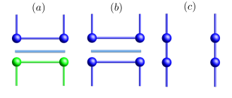
Figure 1: Loop configurations. The cartoons show how the color ($x,y,z$) of a site and its nearest neighbor evolve in a step of imaginary time and how this affects loop decomposition with (a) off-diagonal operators, e.g. $|xx\rangle\langle yy|$ (b) diagonal operators, e.g. $|xx\rangle\langle xx|$, and (c) no operator. In the MC updates, updating the colors of the loops converts between (a) and (b). Dividing or joining loops of the same color converts between (b) and (c). In combination these updates are ergodic. The horizontal bars denote the action of one of the terms in the bond operator, Eq. (3).

The motivation for the “sign-problem” free model we consider here comes from two recently studied materials with Ni²⁺ ions living on a triangular lattice, NiGa₂S₄ [4] and Ba₃NiSb₂O₉ [5]. Both materials are Mott insulators with the Ni²⁺ ions in a $S=1$ state. In surprising discoveries, it was found that both materials have gapless ground states but do not realize the 120^∘ magnetically order state predicted by a semi-classical analysis of the antiferromagnetic Heisenberg model. Despite further investigations, the low temperature phase in these materials is still under debate [6]. Prompted by the experimental work, there has been a number of theoretical studies of $S=1$ models on the triangular lattice, using various approximate methods and exact diagonalization on lattice with up to 21 sites. Depending on the model or method chosen, researchers have found magnetic states, proximity to quantum criticality [7] various spin nematics [8, 9, 10] and spin liquids [11, 12]. One popular theoretical rationalization for the unusual experimental behavior is the presence of a strong biquadratic interaction [13].

Inspired by the extensive experimental and theoretical work we study a $S=1$ model on the triangular lattice with pure biquadratic exchange. Remarkably, we find that this Hamiltonian does not suffer from the sign problem, and exploit this fact to study systems without any approximation on lattices with more than $10^{4}$ spins. Using our numerical results we confirm that the biquadratic model has a spin nematic ground state, consistent with previous approximate studies and small cluster exact diagonalization studies of the same Hamiltonian [10, 8]. We then make accurate estimates for the low energy parameters of this model, thanks to the large system sizes made accesible by our method.

II Model

The model we are interested in can be expressed in terms of the spin-1 Pauli matrices $\vec{S}$ as,

$$\hat{H}=-K\sum_{\langle ij\rangle}\left(\vec{S}_{i}\cdot\vec{S}_{j}\right)^{2}$$ (1)

where the sum is taken over pairs of nearest neighbor sites of a triangular lattice. It is well known that the pure biquadratic model has a staggered SU(3) symmetry on bipartitie lattices. On the non-bipartite triangular lattice studied here it has only the symmetry of spin rotations. In the usual labeling of the eigenstates on a site, the states $|1\rangle,|0\rangle$ and $|\bar{1}\rangle$ are eigenstates of $S_{z}$ with eigenvalues $1,0$ and $-1$. When written in the form above, the model, Eq. (1) appears to have off-diagonal matrix elements with both positive and negative signs, violating the Marshall sign rule. The mappings to follow are most transparent in the orthonormal basis of eigenstates of $S_{x},S_{y}$ and $S_{z}$ with eigenvalue $0$. These are,

$$|x\rangle = \frac{1}{\sqrt{2}}(|1\rangle-|\bar{1}\rangle)$$

$$|y\rangle = \frac{i}{\sqrt{2}}(|1\rangle+|\bar{1}\rangle)$$

$$|z\rangle = |0\rangle$$ (2)

It is possible to verify by inspection that in terms of these basis states the biquadratic operator can be re-written simply as a projector,

$$\left(\vec{S}_{i}\cdot\vec{S}_{j}\right)^{2}-1=3|\mathcal{S}\rangle\langle\mathcal{S}|$$ (3)

where $|\mathcal{S}\rangle=\frac{|xx\rangle+|yy\rangle+|zz\rangle}{\sqrt{3}}$. In this basis it is transparent that the Hamiltonian, Eq. (1), satisfies the Marshall sign criteria, all off-diagonal matrix elements are negative or zero, even on non-bipartite lattices. We note in that although as mentioned above the model does not have all non-positive off diagonal matrix elements in the standard $S_{z}$ basis, this situation can be remedied by the phase rotation $|0\rangle\rightarrow i|0\rangle$, in which case $|\mathcal{S}\rangle=\frac{|00\rangle+|\bar{1}1\rangle+|1\bar{1}\rangle}{\sqrt{3}}$, then from Eq. (3) it has all its matrix elements non-positive.

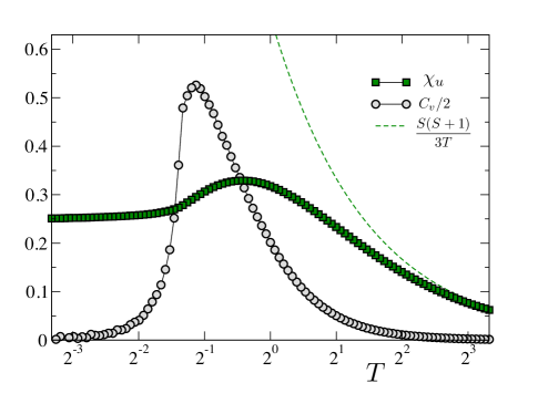
Figure 2: Finite-temperature specific heat, $C_{v}$ (circles) and uniform susceptibility, $\chi_{u}$, (squares) of the $S=1$ biquadratic model, Eq. (1) on a $64\times 64$ triangular lattice. The results are representative of the thermodynamic limit. The single spin Curie law $S(S+1)/3T$ is shown for comparison as a dashed line. We have plotted $C_{v}/2$ to make both data sets fit on the same scale.

The Marshall condition implies that our model Eq. (1) has a positive definite path integral, if we use the $|x\rangle,|y\rangle,|z\rangle$ basis. For concreteness we use the stochastic series expansion (SSE) method to change from Hamiltonian to path integral at finite temperature $T=1/\beta$, in which ${\mathcal{Z}}=\sum_{n}\frac{(-\beta)^{n}}{n!}{\rm Tr}(\hat{H}^{n})$ [14] (The mapping below goes through equally well in the usual Trotter path integral approach). An SSE configuration is specified by assigning to each $\hat{H}$ in the trace one of the terms of Eq. (3) that contributes to the Hamiltonian and its location on the lattice, e.g. $|xx\rangle_{ij}\langle zz|_{ij}$ (see Fig. 1). The partition function is a sum over all SSE configurations, which at any given step in the evaluation of the trace is described by specifying the basis state the system is in at that time slice, i.e., by stating which one of the three colors, $x,y$ or $z$, is on each lattice point. Colors can change through the action of the off-diagonal terms in Eq. (3) in which two neighboring lattice points with the same color can both switch at the next time slice to a new color [see Fig. 1(a)]. It can now be shown that every SSE configuration is identified with a unique loop decomposition: loops are constructed by starting at a point in space-time and moving along the world-line in the time direction until a bond operator is encountered at which point one traverses to the neighboring site on the bond and switches the direction of motion until the loop closes; loops join space-time points with the same color and every space-time point is connected to only one loop (see Ref. [15] for related details). Putting the entire imaginary time history together, it is easy to see that every world-line configuration maps uniquely to a configuration of closed tightly packed loops, each of which is assigned one of three colors, $x,y$ or $z$. The weight of any loop configuration from the stochastic series expansion is then given by the simple formula,

$${\mathcal{Z}}=\sum_{l}\frac{(\beta K)^{n_{l}}}{n_{l}!}3^{{\cal N}_{l}},$$ (4)

where the sum over $l$ is a sum over all closely packed loop configurations, $n_{l}$ is the number of operator insertions (shown in Fig. 1 as horizontal blue bars) and $3^{{\cal N}_{l}}$ is an entropic factor that counts the number of ways colors can be assigned to the ${\cal N}_{l}$ loops in $l$.

III Quantum Monte Carlo

We implement the described mapping of Eq. (1) to a loop model and sampled the SSE configurations with Monte Carlo updates. Loop configurations can be updated by joining loops of the same color, dividing a loop into two smaller loops and changing the color of a loop (see the caption of Fig. 1). Such updates are ergodic and can be chosen with the proper weights to satisfy detailed balance. We note here that past quantum Monte-Carlo work has looked at the biquadratic interaction using a different algorithm in which $S=1$ operators are decomposed into two $S=1/2$ operators as well as a loop algorithm similiar to the one described here, but in the $S^{z}$ basis. These studies were however restricted to bipartite lattices (1-d chains, 2-d square and 3-d cubic lattices) [16, 17, 18].

One can now derive expressions in the loop language for various quantities of interest in the spin model. The total energy $E$ and the specific heat $C_{v}\equiv\frac{1}{N_{s}}\frac{dE}{dT}$ can be measured in the usual manner of the SSE [14]. The uniform susceptibility $\chi_{u}\equiv\frac{\beta}{N_{s}}\left\langle\left(\sum_{i=1}^{N_{s}}S^{z}_{i}\right)^{2}\right\rangle$ can be shown to be exactly $\frac{2}{3}\left\langle\sum_{i}\left(W^{\tau}_{i}\right)^{2}\right\rangle$ where $W^{\tau}_{i}$ is the temporal winding number and $i$ is the index which sums over the loops identified with a given configuration in space-time. The spin stiffness is related to the well known winding number estimator $\rho_{s}=T\left\langle\sum_{i}\left(W^{x}_{i}\right)^{2}\right\rangle$, where $W^{x}$ is the spatial winding number.

We begin by studying the specific heat and the susceptibility of our magnet as it is cooled to its ground state. The data in Fig. 2 on a $64\times 64$ system is representative of the thermodynamic limit. The peak in $C_{v}(T)$ at $T\approx 0.5$ signals the lifting of the extensive entropy of the spins in the high-temperature phase. The observed simultaneous saturation of $\chi_{u}(T)$ is the classic behavior expected of an anti-ferromagnet. Even so, a study of the spin structure factor $S_{S}(\vec{q})\equiv\frac{1}{3L^{2}}\sum_{r}e^{ik\cdot r}\langle\vec{S}(r)\cdot\vec{S}(0)\rangle$, shows no peaks that scale to a finite value in the thermodynamic limit, indicating the absence of simple magnetic long range order as shown in Fig. 3.

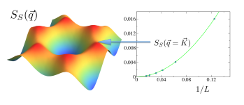
Figure 3: Equal time spin structure factor. (left) Re$[S_{S}(\vec{q})]$ shown in the full first Brillouin zone of the triangular lattice on a $32\times 32$ system at $\beta=32$. (right) the peak height of the structure factor at the corner of the BZ (so-called “K”-point) as a function of inverse system size. The solid circles are the QMC data and the solid line is a numerical fit that shows the spin order vanishes in the thermodynamic limit.

A natural guess for a magnetic state with no Bragg peaks in the spin structure factor is a spin nematic. Such a state breaks spin rotational symmetry but preserves time reversal symmetry. The order parameter for the spin nematic is a traceless symmetric matrix,

$$\hat{Q}_{\alpha\beta}=\frac{\hat{S}_{\alpha}\hat{S}_{\beta}+\hat{S}_{\beta}\hat{S}_{\alpha}}{2}-\frac{2\delta_{\alpha\beta}}{3}.$$ (5)

where $\hat{S}_{\alpha}$ are components of the $S=1$ operator. Since the order parameter is even in the spin operators, its condensation does not imply breaking of time reversal. In order to test for this order we measure the correlation function $C_{Q}(r)=\sum_{\alpha}\langle\hat{Q}_{\alpha\alpha}(r)\hat{Q}_{\alpha\alpha}(0)\rangle$, which is easy to measure in our basis since it is diagonal. It is possible to show that the O(3) invariant correlation function is simply related by a constant, i.e., $C_{Q}(r)=\frac{2}{5}\sum_{\alpha\beta}\langle\hat{Q}_{\alpha\beta}(r)\hat{Q}_{\beta\alpha}(0)\rangle$. Fig. 4(a) shows a plot of $O_{Q}^{2}=\frac{1}{L^{2}}\sum_{r}C_{Q}(r)$ versus $1/L$, keeping the ratio of $K\beta/L=1$ fixed so that we probe the ground state behavior. The finite value for $O_{Q}^{2}$ in the $T=0$ and thermodynamic limit (combined with no condensation in the magnetic structure factor) proves unambiguously that the ground state of our model, Eq. (1), is a spin nematic. It is interesting to ask how much our ground state deviates from a simple product nematic state with no quantum fluctuations, a wavefunction for which is simply, $|\Psi_{\rm prod}\rangle=\prod_{i}|S^{z}=0\rangle_{i}$. In this state the $\langle Q_{\alpha\beta}\rangle=\delta_{\alpha\beta}/3-\delta_{\alpha z}\delta_{\beta z}$, from which we conclude that $(O^{\rm prod}_{Q})^{2}=4/15\approx 0.26666...$. This is the maximum value the order parameter can take, if there are no fluctuations. From the extrapolation in Fig. 4 we find that $(O_{Q})^{2}=0.1376(2)$ in the real ground state, the reduction of about 50% being due to the effect of quantum fluctuations.

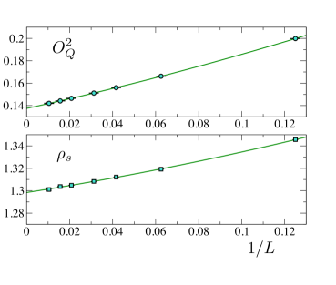
Figure 4: Finite-size scaling at fixed $K\beta/L=1$. The upper panel shows finite size scaling of the data for the nematic order parameter, which in the thermodynamic limit extrapolates to $O_{Q}^{2}=0.1376(2)$. The lower panel shows the extrapolation of the spin stiffness to a value $\rho_{s}=1.298(2)$.

The breaking of the continuous O(3) spin rotational symmetry results in gapless spin waves. Analogous to past work on the Néel state [19] the low energy effective theory of the Goldstone bosons at leading order is characterized completely by just two parameters, the spin stiffness, $\rho_{s}$, and the spin wave velocity, $c$. The stiffness can be estimated by the usual winding number estimator. Fig. 4 (b) shows a plot of $\rho_{s}$ as a function of $1/L$, at fixed $K\beta/L=1$. A finite thermodynamic value for $\rho_{s}$ provides further evidence for gapless spinful excitations at long wavelengths. The spin wave velocity is a number that converts the units of space into the units of time. An estimator for the spin wave velocity, $c$, is hence the ratio of $L/\beta$ at which the anisotropic 2+1 dimensional system behaves cubic. We compute this ratio for each $L$ by adjusting $\beta$ until $\langle{W_{x}}^{2}\rangle=\langle{W_{\tau}}^{2}\rangle$. Then we carry out a thermodynamic extrapolation of the finite size $L/\beta$ data to obtain an estimate for $c$. The data for the winding numbers for a $32\times 32$ system is shown as an example in main panel of Fig. 5. We fit polynomials through this data and estimate the location of the crossing point for each $L$ studied. The value of $L/K\beta$ at the crossing is then plotted versus $1/L$ in the inset. Extrapolating to the thermodynamic limit we obtain that the spin wave velocity, $c=1.869(4)$. The estimates of the order parameter $Q_{\alpha\beta}$, the spin stiffness $\rho_{s}$ and the spin wave velocity $c$, give a complete description of the low energy effective field theory to leading order.

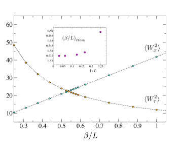
Figure 5: Determination of the spin wave velocity, $c$. In the main panel we show data for the $\langle W_{x}^{2}\rangle$ and $\langle W_{\tau}^{2}\rangle$ on an $L=32$ system as a function of $\beta/L$. In the inset we show how the $\beta/L$ value at the crossing of the types of plots in the main panel scales with system size. These are finite-size estimates for $1/c$, from which we obtain $c=1.869(4)$ in the thermodynamic limit.

IV Summary

In conclusion, we have provided a model $S=1$ hamiltonian with biquadratic interactions that is sign-problem free on non-bipartite lattices. We have shown how the partition function of this model maps to a remarkably simple loop model with positive weights, see Eq. (4). In this publications we studied how this mapping has allowed for a detailed study of the spin nematic ground state on the triangular lattice relevant to many recent experimental and theoretical works and provided high precision estimates for the ground state paramaters. Extensions of the current work to carry out unbiased numerical studies of the role of disorder in quantum spin nematics and deconfined critical points out of the nematic phase [20, 21] are exciting directions for future research. Another field of experiments in which the nematic phase for $S=1$ spins has been discussed is in ultra-cold atoms in optical lattices; it is hoped that our high precision results may be useful for guiding and testing experimental efforts in this context [22].

The author is grateful to Matt Block and Michael Levin for very valuable input, and to Andreas Läuchli for providing ED data used to test the QMC code. The work was supported in part by NSF DMR-1056536.

References

- [1] Leon Balents. Spin liquids in frustrated magnets. Nature, 464(7286):199–208, March 2010.
- [2] U. Schollwöck. The density-matrix renormalization group. Rev. Mod. Phys., 77(1):259–315, 2005.
- [3] R. K. Kaul, R. G. Melko, and A. W. Sandvik. Bridging lattice-scale physics and continuum field theory with quantum monte carlo simulations. Ann. Rev. Cond. Mat. Phys, 2013.
- [4] S Nakatsuji, Y Nambu, H Tonomura, O Sakai, S Jonas, C Broholm, H Tsunetsugu, YM Qiu, and Y Maeno. Spin disorder on a triangular lattice. Science, 309(5741):1697, 2005.
- [5] J. G. Cheng, G. Li, L. Balicas, J. S. Zhou, J. B. Goodenough, Cenke Xu, and H. D. Zhou. High-pressure sequence of structural phases: New quantum spin liquids based on . Phys. Rev. Lett., 107:197204, Nov 2011.
- [6] Satoru Nakatsuji, Yusuke Nambu, Keisuke Onuma, Seth Jonas, Collin Broholm, and Yoshiteru Maeno. Coherent behaviour without magnetic order of the triangular lattice antiferromagnet niga2s4. J. Phys. - Condensed Matter, 19(14), 2007.
- [7] G. Chen, M. Hermele, and L. Radzihovsky. Frustrated quantum critical theory of putative spin-liquid phenomenology in . Phys. Rev. Lett., 109:016402, Jul 2012.
- [8] Andreas Laeuchli, Frederic Mila, and Karlo Penc. Quadrupolar phases of the s=1 bilinear-biquadratic heisenberg model on the triangular lattice. Phys. Rev. Lett., 97(8), 2006.
- [9] Hirokazu Tsunetsugu and Mitsuhiro Arikawa. Spin nematic phase in s=1 triangular antiferromagnets. Journal of the Physical Society of Japan, 75(8), 2006.
- [10] Subhro Bhattacharjee, Vijay B. Shenoy, and T. Senthil. Possible ferro-spin nematic order in niga2s4. Phys. Rev. B, 74(9), 2006.
- [11] Tarun Grover and T. Senthil. Non-abelian spin liquid in a spin-one quantum magnet. Phys. Rev. Lett., 107:077203, Aug 2011.
- [12] Cenke Xu, Fa Wang, Yang Qi, Leon Balents, and Matthew P. A. Fisher. Spin liquid phases for spin-1 systems on the triangular lattice. Phys. Rev. Lett., 108:087204, Feb 2012.
- [13] E. M. Stoudenmire, Simon Trebst, and Leon Balents. Quadrupolar correlations and spin freezing in s=1 triangular lattice antiferromagnets. Phys. Rev. B, 79(21), 2009.
- [14] Anders W. Sandvik. AIP Conf. Proc., 1297:135, 2010.
- [15] Olav F. Syljuåsen and Anders W. Sandvik. Quantum monte carlo with directed loops. Phys. Rev. E, 66(4):046701, Oct 2002.
- [16] Naoki Kawashima and Kenji Harada. Recent developments of world-line monte carlo methods. Journal of the Physical Society of Japan, 73:1379, 2004.
- [17] Kenji Harada and Naoki Kawashima. Loop algorithm for heisenberg models with biquadratic interaction and phase transitions in two dimensions. Journal of the Physical Society of Japan, 70(13), 2001.
- [18] Kenji Harada and Naoki Kawashima. Quadrupolar order in isotropic heisenberg models with biquadratic interaction. Phys. Rev. B, 65(052403), 2002.
- [19] Sudip Chakravarty, Bertrand I. Halperin, and David R. Nelson. Low-temperature behavior of two-dimensional quantum antiferromagnets. Phys. Rev. Lett., 60(11):1057–1060, Mar 1988.
- [20] Kenji Harada, Naoki Kawashima, and Matthias Troyer. Dimer-quadrupolar quantum phase transition in the quasi-one-dimensional heisenberg model with biquadratic interaction. Journal of the Physical Society of Japan, 76(1):013703, 2007.
- [21] Tarun Grover and T. Senthil. Quantum spin nematics, dimerization, and deconfined criticality in quasi-1d spin-one magnets. Phys. Rev. Lett., 98(24):247202, Jun 2007.
- [22] Adilet Imambekov, Mikhail Lukin, and Eugene Demler. Spin-exchange interactions of spin-one bosons in optical lattices: Singlet, nematic, and dimerized phases. Phys. Rev. A, 68(6):063602, Dec 2003.