Topological Aspects of Fermions on Hyperdiamond

Abstract

Motivated by recent results on the index of the Dirac operator $D=\gamma^{\mu}D_{\mu}$ of QCD on lattice and also by results on topological features of electrons and holes of 2-dimensional graphene, we compute in this paper the Index of D for fermions living on a family of even dimensional lattices denoted as $\mathbb{L}_{2N}$ and describing the 2N-dimensional generalization of the graphene honeycomb. The calculation of this topological Index is done by using the direct method based on solving explicitly the gauged Dirac equation and also by using specific properties of the lattices $\mathbb{L}_{2N}$ which are shown to be intimately linked with the weight lattices of $SU\left(2N+1\right)$. The Index associated with the two leading $N=1$ and $N=2$ elements of this family describe precisely the chiral anomalies of graphene and QCD₄. Comments on the method using the spectral flow approach as well as the computation of the topological charges on 2-cycles of 2N-dimensional compact supercell in $\mathbb{L}_{2N}$ and applications to QCD₄ are also given.
Key words: Topological index, Lattice QCD₄, Graphene, Chiral anomaly, Root and Weight lattices of $SU\left(N\right)$, Adam’s spectral flow.      

I Introduction

It is quite well known that the spectrum of the gauged Dirac operator $D=\gamma^{\mu}\left(\partial_{\mu}-iA_{\mu}\right)$ $\equiv\gamma^{\mu}D_{\mu}$ of 2- and 4- dimensional Dirac theories describing the dynamics of fermionic waves $\Psi\left(x\right)$ in a uniform background field with topological charge $Q_{tot}$ obeys the famous Atiyah-Singer index theorem 1A ; 1B ; one of the most substantial achievements of modern mathematics. The index of the Dirac operator $D$, to which we refer below to as $Ind\left(\emph{D}\right)$, relates the topological charge $Q_{tot}$ to the net numbers $N_{+}$ and $N_{-}$ of chiral and antichiral zero modes of $D$ as

$$Q_{tot}=N_{+}-N_{-}$$ (1)

showing in turns that the background field breaks implicitly the left-right parity symmetry. The $Ind\left(\emph{D}\right)$ is a powerful topological quantity that has been used for diverse purposes 2A -2G ; see also  AL and refs therein for other applications; it gives a rigorous explanation of the origin of chiral anomalies and constitutes an alternative approach to the perturbative method based on computing radiative corrections to describe $\bar{\Psi}\gamma^{\mu}\Psi A_{\mu}$ interactions in QFT₁₊₂ where the topological Chern-Simons gauge theory emerges as a 1-loop correction of the gauge field propagator 3A ; 3B . In 2-dimensions, the computation of $Ind\left(\emph{D}\right)$ shows that the anomalous quantum Hall effect (QHE) of graphene 4A ; 4B ; 4C is precisely due to the chiral anomaly of zero modes; a basic result that is expected to be valid as well for higher dimensional Dirac fermions in background fields including light quarks on 4D hyperdiamond 5A -5G and fermions on higher 2N- dimensional honeycombs. Recall by the way that in graphene the quantum Hall effect is a very special effect in the sense it can be observed at room temperature; the gap between the $n=0$ and $n=1$ Landau levels is around 1300K at 10 Tesla compared to around 100K in an ordinary 2D electronic gaz RT ; TR ; see also 17 ; 18 ; 19 ; 20 for other related aspects.

Motivated by recent developments on the index theorem on lattice QCD₄ 6A ; 6B ; 6C ; 6D , we compute in this paper the $Ind\left(\emph{D}_{4}\right)$, and in general the $Ind\left(\emph{D}_{2N}\right)$, of fermions in background fields living on a class of even- dimensional lattices $\mathbb{L}_{2N}$ describing the 2N- dimensional generalization of the honeycomb $\mathbb{L}_{2}$. The calculation of $Ind\left(\emph{D}_{2N}\right)$ will be done as follows:

• use known results on the index to bring the lattice analysis to the spectrum of the fermionic operator near the Fermi level; i.e the spectrum near the Dirac points of lattice QCD_2N where live fermionic zero modes contributing to $Ind\left(\emph{D}_{2N}\right)$.

• then determine these fermionic zero modes by using the direct method based on the two following:
  $\left(a\right)$ using specific features of the $SU\left(2N+1\right)$ roots and weights to deal with the symmetry properties of the lattices $\mathbb{L}_{2N}$ with $N=1,2,...$;
  $\left(b\right)$ solving explicitly the gauged Dirac equation $D\Psi=\epsilon\Psi$, with $\epsilon$ standing for massive deformations around the Fermi level.

Recall that there are two basic ways to compute $Ind\left(\emph{D}_{4}\right)$; $\left(i\right)$ the direct method which we will be considering here; and $\left(ii\right)$ the so called spectral flow approach of Adams 6A ; 6B ; 6C ; 6D based on the introduction of a hermitian version $H_{sp}$ of the Dirac operator. In QCD₄ on hyperdiamond, this spectral hamiltonian has the form $H_{sp}=\gamma_{5}\left(D-m\right)$ showing that any zero mode of $D$ with $\pm$ chirality corresponds to some eigen-modes of $H_{sp}$ with eigenvalues $\lambda\left(m\right)=\mp m$; for details see 6A ; 6B ; 6C ; 6D ; 6DD ; D6 ; 5G .

Our interest into the study of the index of the Dirac operator of fermions on $\mathbb{L}_{2N}$ has been also motivated by the two following:

(1) the 2 leading lattices $\mathbb{L}_{2}$, $\mathbb{L}_{4}$ of the family $\mathbb{L}_{2N}$ are precisely given by the honeycomb of graphene, thought of here as lattice QCD₂, and the 4D hyperdiamond used in lattice QCD₄. So, one expects the members of this family to share some basic features; in particular methods to approach the physical properties of fermions on $\mathbb{L}_{2N}$. This link opens a window for new ways to modeling and simulating in euclidian relativistic theory by borrowing ideas from graphene as done by M. Creutz in 5A ; see also  5B ; 5C ; 5E .

(2) the existence of a remarkable relation between the $\mathbb{L}_{2N}$ honeycomb’s class and the family of weight lattices of the $SU\left(2N+1\right)$ Lie algebras. This extraordinary relation allows a unified description of the tight binding description of fermions on $\mathbb{L}_{2N}$ with $N$ a generic integer; and permits moreover to take advantage of the power of the $SU\left(2N+1\right)$ representations to work out explicit configurations for fermions and gauge fields on $\mathbb{L}_{2N}$. For example boundary conditions of the fields on supercells in $\mathbb{L}_{2N}$ as well as the determination of the Dirac points $\left\{P_{i}\right\}$ regarding fermions on $\mathbb{L}_{2N}$ get mapped to manageable equations on the $SU\left(2N+1\right)$ weight lattice where the duality between simple roots $\mathbf{\alpha}_{i}$ of $SU\left(2N+1\right)$ and its fundamental weight vectors $\mathbf{\omega}_{i}$ plays a crucial role 5E ; 5F ; 5H ; 5I .

Our explicit analysis for computing the index of the Dirac operator allows us as well to get more insight into the structure of the topological index on lattice; in particular into the two following things: (a) the relation between the various possible fluxes $Q_{i}$ through the 2-cycles $C_{i}$ of the supercell compactification and the total charge $Q_{tot}$ of the background fields. (b) the role played by the different matrices $\Gamma_{{}_{2N+1}}$ one can construct from the 2D Pauli ones namely

$$\Gamma_{{}_{2N+1}}=\tau_{{}_{3}}\otimes\left(\sigma_{{}_{3}}\right)^{n_{{}_{1}}}\otimes...\otimes\left(\sigma_{{}_{3}}\right)^{n_{{}_{N-1}}}$$ (2)

with $n_{i}=0,1$ and $\tau_{3}=diag\left(1,-1\right)=\sigma_{3}$.

Regarding the topological charges $Q_{i}$ and $Q_{tot}$, notice that the lattice $\mathbb{L}_{2N}$ is recovered by considering a 2N- dimensional compact supercell with homology classes as those of the real 2N-torus $\mathbb{T}^{2N}$. While in 2-dimensions the homology of the supercell has one 2-cycle given by the parallelogram of fig 3, the situation is richer in higher dimensions. In the case of 4D hyperdiamond for instance, the homology of the 4D compact supercell has, in addition to the real 4-cycle $C_{4}\sim\mathbb{T}^{4}$, a basis of six 2-cycle $C_{i}\sim\mathbb{T}_{i}^{2}$ leading to the following topological charges

$$Q_{tot}=\frac{1}{8\pi^{2}}{\displaystyle\int\nolimits_{C_{4}}}F\wedge F,\qquad Q_{i}=\frac{1}{2\pi}{\displaystyle\int\nolimits_{C_{i}}}F$$

related as in eq(201) and playing a central role in computing the index of the Dirac operator.

Concerning the matrices $\Gamma_{{}_{2N+1}}$ for fermions on 2N-honeycombs, one has in general $2^{N-1}$ possible representations depending on the values of the $n_{i}$’s of (2). For the case of the 4D hyperdiamond, there are two kinds of such matrices and are as follows

$$\gamma_{5}=\sigma_{3}\otimes I,\qquad\sigma_{3}\otimes\tau_{3}.$$

The explicit computation of the Dirac index given in sections 5 and 6 shows that these matrices lead to different relations between the zero modes and the topological charges. We will show that the right index of the Dirac operator that recovers (1) is given by $Tr\left(\bar{\Psi}\sigma_{3}\otimes\tau_{3}\Psi\right)=Q_{top}$.

The presentation is as follows: In section 2, we review the usual approach to honeycomb; but now by using the root and weight lattices of $SU\left(3\right)$; the latter is a hidden symmetry of the honeycomb. In section 3, we study the topological aspects of fermions in graphene in presence of an external magnetic field $B$ and develop the explicit computation of the zero modes of the gauged Dirac operator. As we will show, the basic properties of the ground state are encoded in the sign $\frac{B}{\left|B\right|}$ of the background field. In section 4, we use the results on graphene to approach the fermions on hyperdiamond in presence of two background fields $B$ and $E$. In this study, we also use roots and weight lattices of $SU\left(5\right)$ that appears as a hidden symmetry of the 4D crystal. In section 5, we compute the spectrum of the Dirac operator in continuum, and in section 6 we work out the complete spectrum of fermions on the hyperdiamond lattice. We also compute the topological index giving the relation between the zero modes and the various topological charges of the background fields. Here also, we show that the ground state features are encoded in the sign of $\frac{B}{\left|B\right|}$ and $\frac{E}{\left|E\right|}$. In section 7, we give a conclusion and make comments on the extension to fermions on 2N- dimensional honeycomb in presence of N background fields $B_{i}$ whose signs $\frac{B_{i}}{\left|B_{i}\right|}$ characterize completely the ground states.

Before proceeding, we would like to notice that we will omit certain technical details on lattice calculations from the core of the paper; the essential of these details is reported in appendix 8; and related extensions can be found in 5A ; 5B ; 5C ; 5D ; 5E ; TB ; PSM .

II Fermions on 2D honeycomb

In this section, we develop the so called primitive compactification of fermion on honeycomb used in 4C to study topological aspects of fermions in graphene. To get more insight into our analysis, we first describe the canonical frame formulation, generally used to deal with fermions on square lattice; then we turn back to study the primitive frame (P-frame) and exhibit its link with the root and the weight lattices of the $SU\left(3\right)$ Lie algebra. This study can be also viewed as a step to fix the ideas before moving to the case of QCD₄ fermions on hyperdiamond to be considered in sections 4, 5 and 6.

II.1 2D honeycomb and $SU\left(3\right)$ weight lattice

Honeycomb is a 2D lattice where each site has 3 first nearest neighbors and 6 second nearest ones as shown on fig 1; the 3 first neighbors will be viewed here as the vertices of an equilateral triangle transforming as a $SU\left(3\right)$ triplet; and the second 6 ones the vertices of an hexagon. The lattice parametrization of the honeycomb can be obtained from the real plane $\mathbb{R}^{2}$ by restricting the local real coordinate $\mathbf{r}=\left(X,Y\right)$ to $\mathbf{r}_{n,m}=\left(X_{n},Y_{m}\right)$ with $n,m$ integers. As a 2D vector, one may expand the position vector $\mathbf{r}$ in diverse ways; in particular into 2 particular frames used in 4C and named there as perpendicular frame and primitive one; see fig 1 for illustration. Here, we will refer to the perpendicular frame as the canonical one.

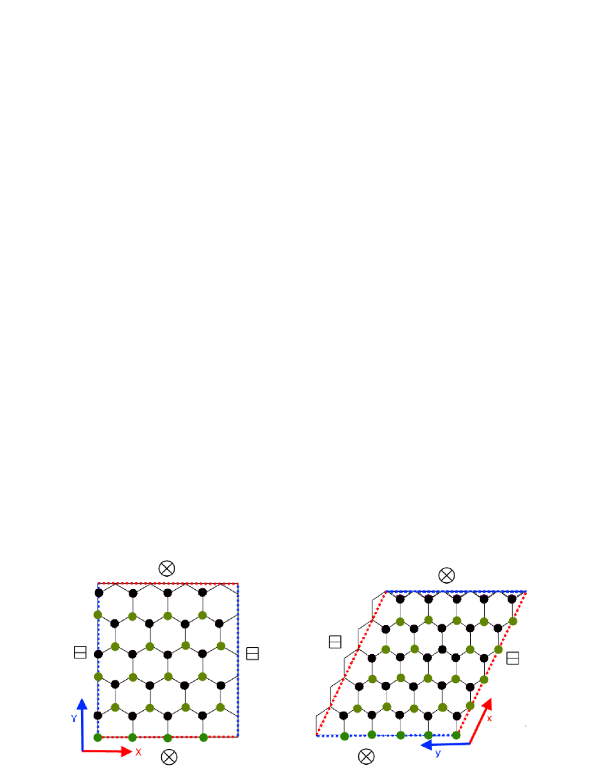
Figure 1: On left the perpendicular compactification. On right the primitive compactification

• Canonical compactification

In the canonical compactification (C-frame), one uses the usual orthogonal cartesian basis $\left\{\mathbf{e}_{X},\mathbf{e}_{Y}\right\}$ of $\mathbb{R}^{2}$ to decompose vectors like $\mathbf{r}=X\mathbf{e}_{X}+Y\mathbf{e}_{Y}$,

$$\mathbf{e}_{\mu}.\mathbf{e}_{\mu}=\delta_{\mu\nu}$$ , , .

       (3)

The restriction of local fields $F\left(\mathbf{r}\right)$ to the honeycomb is obtained by using the Dirac delta function $\delta\left(\mathbf{r-r}_{n,m}\right)$ as

$$F_{\mathbf{r}_{n,m}}=\int_{\mathbb{R}^{2}}d^{2}\mathbf{r}\text{ }\delta\left(\mathbf{r-r}_{n,m}\right)F\left(\mathbf{r}\right).$$ (4)

The dynamics of fermionic waves $\Psi\left(T,X,Y\right)$ describing the delocalized electrons near the Dirac points is given by the Dirac equation

$$\left(\gamma^{0}\frac{\partial}{\partial T}+\gamma^{1}\frac{\partial}{\partial X}+\gamma^{2}\frac{\partial}{\partial Y}\right)\Psi=0,$$ (5)

with

$$\gamma^{0}=\left(\begin{array}[c]{cc}1&0\\ 0&-1\end{array}\right),$$

       (6)

satisfying the Clifford algebra in $\left(2+1\right)$-dimensions. The solutions of this equation are given by plane waves $e^{ik_{T}T-i\left(k_{X}X+k_{Y}Y\right)}$ with $k_{T}^{2}=k_{X}^{2}+k_{Y}^{2}$. Boundary conditions such as $\Psi\left(T,X+L,Y\right)$ $=\Psi\left(T,X,Y\right)$ leads to discrete $K_{X}=\frac{2\pi n}{L}$, $n\in\mathbb{Z}$.

• Primitive compactification

In the primitive frame (P-frame) of honeycomb, one uses the non orthogonal vector basis

$$\mathbf{e}_{x}\mathbf{.e}_{x}=1$$ ,

,

(7)

allowing to take advantage of the two following remarkable features of the honeycomb:

(i) honeycomb contains the root lattice of SU$\left(3\right)$
The basis vectors $\mathbf{e}_{x}\mathbf{,}$ $\mathbf{e}_{y}$ are, up to a scale factor, precisely the simple roots $\mathbf{\alpha}_{1}$ and $\mathbf{\alpha}_{2}$ of the $SU\left(3\right)$ Lie algebra

$$\mathbf{e}_{x}=\frac{\sqrt{2}}{2}\mathbf{\alpha}_{1},\qquad\mathbf{e}_{y}=\frac{\sqrt{2}}{2}\mathbf{\alpha}_{2}$$

so that space vectors like positions can be decomposed as

$$\mathbf{r}$$ .

   (8)

The relation between the C- and P- frames is given by

$$X^{\mu}$$ ,

,

(9)

or by using matrices

$$\left(\begin{array}[c]{c}X\\ Y\end{array}\right)=\frac{\sqrt{2}}{2}\left(\begin{array}[c]{cc}\alpha_{1}^{1}&\alpha_{1}^{2}\\ \alpha_{2}^{1}&\alpha_{2}^{2}\end{array}\right)\left(\begin{array}[c]{c}x\\ y\end{array}\right).$$ (10)

The inverse transformation is

$$\left(\begin{array}[c]{c}x\\ y\end{array}\right)=\sqrt{2}\left(\begin{array}[c]{cc}\beta_{1}^{1}&\beta_{1}^{2}\\ \beta_{2}^{1}&\beta_{2}^{2}\end{array}\right)\left(\begin{array}[c]{c}X\\ Y\end{array}\right),$$ (11)

with the constraint $\beta_{\mu}^{i}\alpha_{i}^{\nu}=\delta_{\mu}^{\nu}$ which is solved in terms of the $\alpha_{i}^{\mu}$’s like

$$\beta_{\mu}^{i}=\frac{1}{\Delta}\varepsilon_{\mu\nu}\varepsilon^{ji}\alpha_{j}^{\nu}$$

with $\Delta=\det\left(\alpha_{i}^{\mu}\right)=\frac{1}{2}\varepsilon_{\mu\nu}\varepsilon^{ji}\alpha_{j}^{\nu}\alpha_{i}^{\mu}$.

(ii) honeycomb is the weight lattice of SU$\left(3\right)$
The matrix $\beta_{\mu}^{i}$ is precisely the entries of the fundamental weight vectors of $SU\left(3\right)$

$$\mathbf{\omega}^{1}=\left(\beta_{\mu}^{1}\right),\qquad\mathbf{\omega}^{2}=\left(\beta_{\mu}^{2}\right)$$

These vectors are dual to the simple roots

$$\mathbf{\alpha}_{i}.\mathbf{\omega}^{j}=\delta_{i}^{j}.$$

Notice that the roots of Lie algebras can be expanded in terms of the weight vectors and vice versa. For the example of SU$\left(3\right)$, the simple roots decompose as

$$\mathbf{\alpha}_{1}=2\mathbf{\omega}^{1}-\mathbf{\omega}^{2},\qquad\mathbf{\alpha}_{2}=2\mathbf{\omega}^{2}-\mathbf{\omega}^{1}$$

This features teaches as that honeycomb sites are given by $n_{1}\mathbf{\omega}^{1}+n_{2}\mathbf{\omega}^{2}$ with $n_{i}$ arbitrary integers. Moreover sites in the sublattices $\mathbb{A}$ and $\mathbb{B}$ of honeycomb are rather given by $n_{1}\mathbf{\alpha}_{1}+n_{2}\mathbf{\alpha}_{2}.$

(iii) from 2D honeycomb to 4D hyperdiamond
The link between honeycomb and the root lattice of $SU\left(3\right)$ is very suggestive. It allows to extend results on 2D graphene to fermions on higher 2N- dimensional lattices. The latters are isomorphic to the weight lattice of $SU\left(2N+1\right)$ Lie algebras and permits the following correspondence

N $$\ {\small SU}\left(2N+1\right)$$                            Lattice

1 2D honeycomb of graphene

2 4D honeycomb  4D hyperdiamond of QCD₄

3 6D honeycomb

    

In this view, 2D graphene appears as the leading term of a family of lattice models. The second element of this family is remarkably given by the 4D hyperdiamond that is used in dealing with quarks in lattice QCD₄ 5A -5G .

To make contact with the study of 4C , we take the components of the simple roots in the C-frame as,

$$\mathbf{\alpha}_{1}=\left(\frac{\sqrt{2}}{2},\frac{\sqrt{6}}{2}\right),$$

             (12)

leading to

$$\alpha_{i}^{\mu}=\left(\begin{array}[c]{cc}\frac{\sqrt{2}}{2}&\frac{\sqrt{6}}{2}\\ -\sqrt{2}&0\end{array}\right),$$

(13)

with $\mathbf{\alpha}_{1}\wedge\mathbf{\alpha}_{2}=$ $\Delta=\sqrt{3}$; and

$$\mathbf{\omega}^{1}=\left(0,\frac{\sqrt{6}}{3}\right)$$ ,

             (14)

with $\mathbf{\omega}_{1}\wedge\mathbf{\omega}_{2}=\frac{\sqrt{3}}{3}$ which is $\frac{1}{3}$ smaller compared to $\mathbf{\alpha}_{1}\wedge\mathbf{\alpha}_{2}$. Notice that the transpose vectors

$$\mathfrak{a}^{1}=\left(\alpha_{i}^{1}\right)=\left(\frac{\sqrt{2}}{2},-\sqrt{2}\right)$$ ,

,

(15)

satisfy as well the duality duality relation $\mathfrak{a}^{\mu}.\mathfrak{b}_{\nu}=\delta_{\nu}^{\mu}$. Notice also that the vectors $\mathbf{\hat{0}}$, $\mathbf{\hat{1}}$, $\mathbf{\hat{2}}$ used in 4C are nothing but the three 3 roots SU$\left(3\right)$ namely $\mathbf{\alpha}_{1},$ $\mathbf{\alpha}_{2},$ $\mathbf{\alpha}_{3}=\mathbf{\alpha}_{1}+\mathbf{\alpha}_{2}$; see also fig 2 for illustration.

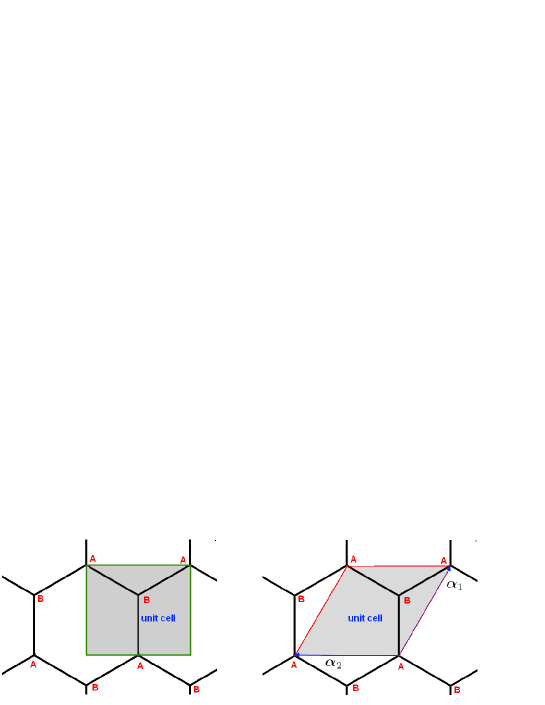
Figure 2: The real unit cell of the 2D honeycomb in C- and P- frames. Sites $A$ (resp $B$) belong to sublattice $\mathbb{A}$ (resp $\mathbb{B}$) of the honeycomb.

The area of the unit cell in the C-frame is given by $L_{1}L_{2}$ and in the P-frame is $l_{1}l_{2}\frac{\sqrt{3}}{2}$. The equality of these areas can checked by using eqs(9,12).

II.2 Dirac equation in primitive frame

One of the lessons we have learned from above is that simple roots $\mathbf{\alpha}_{i}$ and fundamental weight vectors of $\mathbf{\omega}^{i}$ are appropriate tools to deal with fermionic waves on honeycomb and reciprocal space. Real positions $\mathbf{r}$ and wave vectors $\mathbf{k}$ in the momentum space can be decomposed as,

$$\mathbf{r}=x^{i}\mathbf{\alpha}_{i}$$ ,

,

     (16)

The respective norms read as $\mathbf{r}^{2}=C_{ij}x^{i}x^{j}$, $\mathbf{k}^{2}=G^{ij}k_{i}k_{j}$ with metrics $C_{ij}=\mathbf{\alpha}_{i}.\mathbf{\alpha}_{i}$ and $G^{ij}=\mathbf{\omega}^{i}.\mathbf{\omega}^{j}$ given by

$$C_{ij}=\left(\begin{array}[c]{cc}2&-1\\ -1&2\end{array}\right)$$ ,

     (17)

Plane waves $e^{i\mathbf{k.r}}$ which read in C-frame as $e^{iK_{\mu}X^{\mu}}$ takes also the form $e^{ik_{i}x^{i}}$ in the P-frame because of the duality relation $\mathbf{\omega}^{i}.\mathbf{\alpha}_{j}=\delta_{j}^{i}$ appearing in $\exp i\left[\mathbf{\omega}^{i}.\mathbf{\alpha}_{j}\text{ }k_{i}x^{j}\right]$. The Fourier transform reads as usual

$$f\left(\mathbf{r}\right)=\int\frac{d^{2}\mathbf{k}}{\left(2\pi\right)^{2}}F\left(\mathbf{k}\right)e^{i\mathbf{k.r}},$$ (18)

and the gradients are related as $\frac{\partial}{\partial X^{\mu}}=\omega_{\mu}^{i}\frac{\partial}{\partial x^{i}}$ and $\frac{\partial}{\partial x^{i}}=\alpha_{i}^{\mu}\frac{\partial}{\partial X^{\mu}}$. The two sublattices $\mathbb{A}$ and $\mathbb{B}$ of the 2D honeycomb are as follows

$$\mathbb{A}:$$

    

where $\mathbf{a}_{i}=d\sqrt{\frac{3}{2}}\mathbf{\alpha}_{i}\equiv$ $\frac{a}{\sqrt{2}}\mathbf{\alpha}_{i}$ with $d$ standing for the lattice parameter and $n=\left(n_{1}\mathbf{,}n_{2}\right)\in\mathbb{Z}^{2}$. The area of the unit cells in real and momentum spaces are given by

$$\left|\mathbf{a}_{1}\mathbf{\wedge a}_{2}\right|$$

(19)

with $\mathbf{b}_{i}=\frac{2\pi}{d}\sqrt{\frac{2}{3}}\mathbf{\omega}^{i}\equiv$ $\frac{2\pi\sqrt{2}}{a}\mathbf{\omega}^{i}$ the dual vectors of $\mathbf{a}_{i}$. For a real supercell

$$SC_{2}=\left(N_{1}\mathbf{a}_{1}\right)\times\left(N_{2}\mathbf{a}_{2}\right)$$

described by a parallelogram with edges $\mathbf{l}_{i}=N_{i}\mathbf{a}_{i}$, the real area $\mathcal{S}$ is given by $\mathcal{S}=N_{1}N_{2}a^{2}\frac{\sqrt{3}}{4}$.
The dynamics of fermionic waves in the C-frame is given by the Dirac equation $\gamma^{\mu}\frac{\partial}{\partial X^{\mu}}\Psi=0$; it reads in the P-frame as,

$$\left(\Upsilon^{0}\frac{\partial}{\partial t}+\Upsilon^{1}\frac{\partial}{\partial x}+\Upsilon^{2}\frac{\partial}{\partial y}\right)\Psi=0$$ (20)

with the new $\Upsilon^{i}$ Dirac matrices related to the $\gamma^{\mu}$’s like

$$\Upsilon^{i}=\omega_{\mu}^{i}\gamma^{\mu}$$ , ,

     (21)

and obeying the following Clifford algebra

$$\left\{\Upsilon^{i},\Upsilon^{j}\right\}=2G^{ij}$$ ,

.

     (22)

III Topological aspects of fermion on honeycomb

First we give some general features regarding fermion on supercell; then we study the spectrum of the Dirac equation of these fermions in a uniform background field $B$. After that, we compute the index of the Dirac operator in presence of $B$.

III.1 Fermions on supercell

To study the topological aspects of fermions on honeycomb, one has to transcribe the expressions of the usual fields $\Psi\left(\mathbf{x}\right)$ and $A_{\mu}\left(\mathbf{x}\right)$ in the continuum to the case of the lattice. This extension is not straightforward because the field expressions seem to be in conflict with the lattice periodicity. Below, we study this issue by working in the P-frame of the honeycomb and by using its underlying $SU\left(3\right)$ symmetry.

III.1.1 Supercell in honeycomb

The sites of a honeycomb supercell $SC_{2}$ are of two types: A-type and B-type; and are defined as,

$$SC_{2}=\left\{\mathbf{r}_{n}^{\mathbb{A}}=n_{1}\mathbf{a}_{1}+n_{2}\mathbf{a}_{2}\begin{tabular}[c]{l}\\ \end{tabular}\right\}\cup\left\{\mathbf{r}_{n}^{\mathbb{B}}=(n_{1}+\frac{2}{3})\mathbf{a}_{1}+(n_{2}+\frac{1}{3})\mathbf{a}_{2}\begin{tabular}[c]{l}\\ \end{tabular}\right\}$$ (23)

with $n=\left(n_{1},n_{2}\right)$ integers restricted as

$$0\leq n_{i}\leq N_{i}-1$$ , .

(24)

The vectors $\mathbf{r}_{\left(n_{1},0\right)}^{\mathbb{A}}$ and $\mathbf{r}_{\left(0,n_{2}\right)}^{\mathbb{A}}$ are the lattice positions along the $\mathbf{a}_{1}$ and $\mathbf{a}_{2}$ directions with $N_{1}$, $N_{2}$ the respective number of sites in these directions. So the total number of the A-type sites in the supercell is $N_{1}N_{2}$ and then the total area $\mathcal{S}$ of the supercell is equal to $N_{1}N_{2}\frac{a^{2}\sqrt{3}}{2}$. Notice also that in the supercell $SC_{2}$ we also have B-type sites $\mathbf{r}_{\left(n_{1},n_{2}\right)}^{\mathbb{B}}$ with same number as the A-type ones so that the total sites in the supercell is

$$2N_{1}N_{2}.$$ (25)

Notice that the $\mathbf{r}_{\left(n_{1},n_{2}\right)}^{\mathbb{B}}$ sites are shifted with respect to the $\mathbf{r}_{\left(n_{1},n_{2}\right)}^{\mathbb{A}}$ sites by a constant vector as $\mathbf{r}_{n}^{\mathbb{B}}=\mathbf{r}_{n}^{\mathbb{A}}+\mathbf{s}$ with $\mathbf{s=}\frac{2}{3}\mathbf{a}_{1}+\frac{1}{3}\mathbf{a}_{2}$.

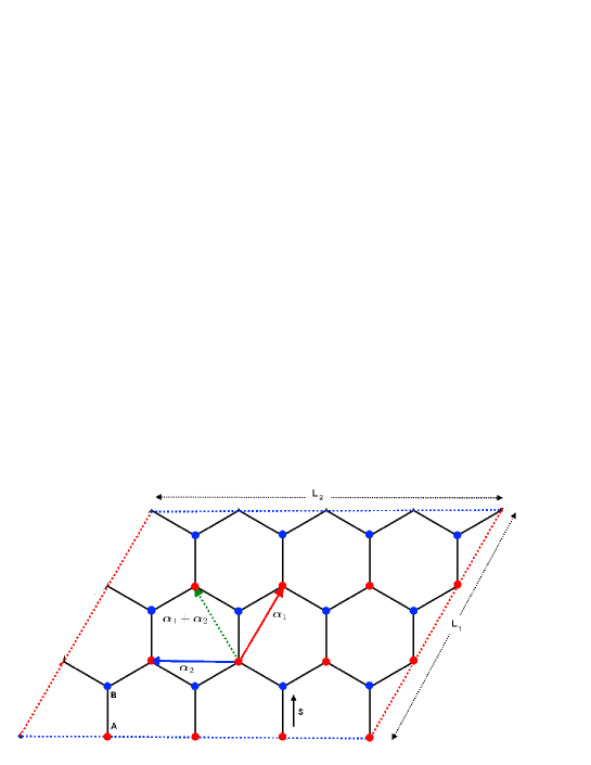
Figure 3: A supercell in primitive compactification; it has 24 sites: 12 sites are A-type (balls in red) and the 12 others of B-type (balls in blue). The origin of the primitive frame belongs to $\mathbb{A}$-sublattice. A shift by the vector $\mathbf{s}$ maps A-type sites into B-type ones.

This shift vector $\mathbf{s}$ has two remarkable features: first it is independent of the site positions $\left(n_{1},n_{2}\right)$; and second it is proportional to $\mathbf{\omega}^{1}=\frac{2}{3}\mathbf{\alpha}_{1}+\frac{1}{3}\mathbf{\alpha}_{2}$; we have $\mathbf{s}=d\sqrt{\frac{3}{2}}\mathbf{\omega}^{1}$. Using the parametrization of 4C , one can check that $\mathbf{\omega}^{1}=(0,\frac{\sqrt{6}}{3})$ and by substituting back into the expression of the shift vector, we get

$$\mathbf{s}=\left(\begin{array}[c]{c}0\\ d\end{array}\right)$$ (26)

III.1.2 Gauge field and fermionic waves on supercell

To deal with the Dirac equation on honeycomb supercell in presence of the background field $B$, one has to worry about the boundary conditions of the gauge field and the fermionic waves under lattice periodicity

$$\mathbf{r}_{n}\rightarrow\mathbf{r}_{n}+nN_{1}\mathbf{a}_{1}+mN_{2}\mathbf{a}_{2},\qquad n,m\in\mathbb{Z}$$ (27)

Constructions regarding this issue has been first done by Smit, J.C. Vink in B2 by working in the C-frame of a square lattice; see also 4C ; 5G . Below we extend this analysis to the P-frame; this is helpful when we consider the extension to QCD₄ on 4D hyperdiamond and extension to higher dimensional lattices.

• Periodicity of the gauge field

In the canonical frame, the gauge field is given by the vector $A_{\mu}$ while in the primitive frame, it is denoted as $\mathcal{A}_{i}$. These two fields capture the same physical property; they are related as $A_{\mu}=\omega_{\mu}^{i}\mathcal{A}_{i}$ or inversely $\mathcal{A}_{i}=\alpha_{i}^{\mu}A_{\mu}$.
Here, we use the P-frame coordinates $x^{i}=\left(x,y\right)$ and work with the gauge covariant derivatives $\mathcal{D}_{i}=\frac{\partial}{\partial x^{i}}-i\mathcal{A}_{i}$ with curvature

$$\left[\mathcal{D}_{i},\mathcal{D}_{j}\right]=-i\mathcal{F}_{ij}=i\varepsilon_{ij}B$$ (28)

related to the C-frame one $\left[D_{\mu},D_{\nu}\right]=-iF_{\mu\nu}$ like

$$\mathcal{F}_{ij}=\alpha_{i}^{\mu}\alpha_{j}^{\nu}F_{\mu\nu}$$

As usual, the gauge field $\mathcal{A}_{i}$ is defined up to gauge transformations $\mathcal{A}_{i}^{\Omega}=$ $\mathcal{A}_{i}+i\Omega\partial_{i}\Omega^{-1}$ where $\Omega=e^{-i\lambda\left(\mathbf{x}\right)}$ is a $U\left(1\right)$ gauge group element with gauge parameter $\lambda\left(\mathbf{x}\right)$. We also have:

$$\Psi^{\Omega}\left(\mathbf{x}\right)$$

       (29)

Since $B$ is constant, a typical gauge configuration of $\mathcal{A}_{i}$ that solve (28) in the continuum is as follows,

$$\mathcal{A}_{x}\left(x,y\right)=\frac{1}{2}By$$ , .

       (30)

This not unique since a different, but equivalent, gauge field representation with curvature $B$ is given by the following simpler one used by Smit, J.C. Vink in B2 ,

$$\mathcal{A}_{x}\left(x,y\right)=0$$ , .

       (31)

However, this gauge field configuration, which is valid in the continuous case, has to be adapted to the lattice; neither (30) nor (31) is periodic on the honeycomb since

$$\mathcal{A}_{i}\left(x+L_{1},y\right)$$ ,

.

(32)

Explicitly, by using the expression (30) for the gauge field $\mathcal{A}_{i}$, we have

$$\mathcal{A}_{x}\left(x,y\right)|_{y=L_{2}}=\frac{BL_{2}}{2}$$ , ,

, .

(33)

If using the gauge configuration (31), we also have

$$\mathcal{A}_{x}\left(x,y\right)|_{y=L_{2}}=0$$ , ,

, .

(34)

To overcome this difficulty, we use the gauge symmetry freedom to ensure field’s periodicity. This is done by requiring

$$\mathcal{A}_{x}\left(x,y\right)|_{y=0}$$ ,

,

(35)

where now the gauge group parameter $\lambda\left(x,y\right)$ is no longer an arbitrary function as in the continuum; this is the price to pay to implement lattice periodicity.
In what follows, we choose the gauge configuration (31) used by Smit and Vink for the case of gauge fields on square lattice. This choice is tricky and allows tremendous simplifications when computing the spectrum of the Dirac operator; especially the degeneracy of the ground state. Using this choice the gauge covariant derivatives reduce to,

$$\mathcal{D}_{x}=\frac{\partial}{\partial x}$$ , ,

      

with no gauge component along the x-direction. In this case, the periodicity condition on the gauge field namely

$$\mathcal{G}_{y}\left(x,y\right)|_{x=0}=\mathcal{G}_{y}\left(x,y\right)|_{x=L_{1}}+\partial_{y}\lambda$$

leads to $\partial_{y}\lambda=BL_{1}$ and then to $\lambda=BL_{1}y+\varphi\left(x\right)\equiv\vartheta\left(y\right)+\varphi\left(x\right)$ with $\varphi$ a real function in the $x$-variable that we shall ignore below as it doesn’t affect the analysis . Notice that as a function on lattice, the gauge symmetry element $\Omega$, thought of as a function of the y-variable only, i.e: $\Omega=\Omega\left(y\right)$, should be also periodic $\Omega\left(y+L_{2}\right)=\Omega\left(y\right)$. The solving of this condition requires the quantization of the background field as

$$BL_{1}L_{2}=2\pi Q$$ , .

       (36)

So the gauge group element reads as

$$\Omega\left(y\right)=\exp\left(-i\frac{2\pi Q}{L_{2}}y\right)$$ ,

       (37)

and can be thought of as describing a wave plane propagating along the y-direction with the momentum $K_{y}=\frac{2\pi Q}{L_{2}}$. This property teaches us that gauge transformations are generated by the shifts

$$p_{y}\rightarrow p_{y}+n\frac{2\pi Q}{L_{2}},\qquad n\in\mathbb{Z}$$ (38)

of the momenta $p_{y}=\frac{2\pi l}{L_{2}}$ along the y-axis.

• Periodicity of fermionic waves

Fermionic waves $\Psi\left(x,y\right)$ on honeycomb supercell have to obey consistent boundary conditions. Because of gauge freedom, the boundary condition should be as

$$\Psi\left(x+nL_{1},y+mL_{2}\right)=\mathcal{R}_{n,m}\Psi\left(x,y\right),$$

where $\mathcal{R}_{n,m}$ is some representation of the gauge symmetry which is given by some local phase $e^{i\vartheta_{n,m}\left(y\right)}$. However, with the gauge choice (31), these condition reduces to

$$\Psi\left(x,y=L_{2}\right)$$ ,

.

       (39)

To get the explicit expression of the fermionic waves, one has to solve the Dirac equation on the lattice; this will be done in next subsection; for the moment we use general arguments to derive some useful information on these waves.
First, because of the choice (31) where the gauge field $\mathcal{A}_{i}$ has no dependence in the y- variable, the periodicity condition of fermionic waves namely $\Psi\left(x,y+L_{2}\right)=\Psi\left(x,y\right)$ can be solved in terms of plane waves propagating along the y-direction as follows

$$\Psi\left(x,y\right)={\displaystyle\sum\limits_{l\in\mathbb{Z}}}e^{i\frac{2\pi l}{L_{2}}y}\Psi_{l}\left(x\right)$$ (40)

The Fourier modes $\Psi_{l}\left(x\right)$, which depend on $x$, carry an integer charge $l$ and because of the second condition of (39) are expected to be not completely independent fields.
Second, to solve the boundary condition along the x-direction, we expand the wave function at $x+L_{1}$ in a similar manner as in (40)

$$\Psi\left(x+L_{1},y\right)={\displaystyle\sum\limits_{l\in\mathbb{Z}}}e^{i\frac{2\pi l}{L_{2}}y}\Psi_{l}\left(x+L_{1}\right)$$ (41)

and then require that the value of the fermionic waves at the equivalent positions $x$ and $x+L_{1}$ to be related by a gauge transformation like $\Psi\left(x,y\right)=$ $e^{-iBL_{1}y}$ $\Psi\left(x+L_{1},y\right)$. This leads to the following relation between the Fourier modes,

$$\Psi_{l}\left(x+L_{1}\right)=\Psi_{l-Q}\left(x\right)$$ (42)

This property can be exhibited by help of the quantization relation $2\pi Q=BL_{1}L_{2}$ allowing to express the wave plane basis $e^{i\frac{2\pi l}{L_{2}}y}$ in terms of the magnetic field and the topological charge like $e^{iBL_{1}\frac{l}{Q}y}$. Substituting this expression back into (40), one ends with (42). Notice that eq(42) is solved by taking

$$\Psi_{l}\left(x\right)=\Phi\left(x+\frac{l}{Q}L_{1}\right)$$ (43)

showing that a translation $y\rightarrow y+L_{2}$ along the y-direction by one period induces the shift $x\rightarrow x+\frac{1}{Q}L_{1}$ along the x-axis. The explicit expression of the function $\Phi\left(\xi\right)$ will be determined below.

III.2 Index of Dirac operator and chiral anomaly

In the P-frame of the honeycomb, the Dirac equation of the two component fermionic wave $\Psi=\left(\psi,\chi\right)$ in the background field $B$ is given by the following $2\times 2$ matrix equation

$$\Upsilon^{i}\mathcal{D}_{i}\left(\begin{array}[c]{c}\psi\\ \chi\end{array}\right)=iE\Upsilon^{0}\left(\begin{array}[c]{c}\psi\\ \chi\end{array}\right),$$ (44)

where $\Upsilon^{0}$, $\Upsilon^{1}$, $\Upsilon^{2}$ are $2\times 2$ gamma matrices which are related to the usual gamma matrices $\gamma^{\mu}$ as in (21).

III.2.1 Solving Dirac equation on supercell

The gauge covariant derivatives $\mathcal{D}_{i}=\partial_{i}-i\mathcal{A}_{i}$ with $\mathcal{A}_{i}$ taken the SV gauge are as follows

$$\mathcal{D}_{1}=\frac{\partial}{\partial x}$$ , ,

(45)

with no component $\mathcal{A}_{x}$ for the gauge vector. Using the expression of $\gamma^{0}=\sigma^{3}$, $\gamma^{1}=i\sigma^{1}$, $\gamma^{2}=i\sigma^{2}$ with the Pauli matrices $\sigma^{\mu}$ as in eq(6), the matrices $\Upsilon^{i}$ read as:

$$\Upsilon^{1}=i\left(\begin{array}[c]{cc}0&\xi\\ \bar{\xi}&0\end{array}\right),$$

(46)

where we have set $\xi=\omega_{1}^{1}-i\omega_{2}^{1}$, $\zeta=\omega_{1}^{2}-i\omega_{2}^{2}$ with the useful relations

$$\xi\bar{\xi}=\left\|\mathbf{\omega}^{1}\right\|^{2}$$ , .

,

(47)

By replacing the weight vectors $\mathbf{\omega}^{i}$ by their expression (14), reads as

$$\xi\bar{\xi}=\frac{2}{3}$$ ,

,

(48)

Notice that like in the C-frame, the Dirac operator $\Upsilon^{i}\mathcal{D}_{i}$ in presence of the background field B can be put as well into the form

$$\Upsilon^{i}\mathcal{D}_{i}=i\left(\begin{array}[c]{cc}0&D\\ \bar{D}&0\end{array}\right)$$ ,

(49)

with $D=\xi\mathcal{D}_{1}+\zeta\mathcal{D}_{2}$ and $\bar{D}=\bar{\xi}\mathcal{D}_{1}+\bar{\zeta}\mathcal{D}_{2}$. Its square, which is needed for solving the Dirac equation, is diagonal

$$\left(\Upsilon^{i}\mathcal{D}_{i}\right)^{2}=-\left(\begin{array}[c]{cc}D\bar{D}&0\\ 0&\bar{D}D\end{array}\right)$$ ,

(50)

and has the same eigen wave functions as $\Upsilon^{i}\mathcal{D}_{i}$. Notice also that the explicit expression of $D$ and $\bar{D}$ are as

$$D$$ ,

,

(51)

and satisfy the commutation relation

$$\left[D,\bar{D}\right]=-iB\left(\xi\bar{\zeta}-\bar{\xi}\zeta\right)=-\frac{2B\sqrt{3}}{3}$$ ,

   (52)

where the sign of the right hand side depends on the sign of $B$; it is positive if sign$\left(B\right)$ is negative and vice versa.

III.2.2 The explicit spectrum

Setting

$$D=\sqrt{\frac{2\left|B\right|\sqrt{3}}{3}}A^{-}$$ ,

     (53)

the commutation relation (52) becomes

$$\left[A^{-},A^{\dagger}\right]=-\frac{B}{\left|B\right|}I$$ ,

     (54)

with the remarkable dependence in $\frac{B}{\left|B\right|}$ capturing the sign of the background field $B$. By substituting back into (50), the squared Dirac operator reads as

$$\left(\begin{array}[c]{cc}D\bar{D}&0\\ 0&\bar{D}D\end{array}\right)=\frac{2\left|B\right|\sqrt{3}}{3}\left(\begin{array}[c]{cc}A^{-}A^{\dagger}&0\\ 0&A^{\dagger}A^{-}\end{array}\right)$$ ,

(55)

To get the solution of the Dirac equation, we first use the periodicity condition along the y-axis to expand the fermionic wave $\Psi\left(x,y\right)$ in Fourier series like

$$\Psi\left(x,y\right)={\displaystyle\sum\limits_{l\in\mathbb{Z}}}e^{i\frac{2\pi l}{L_{2}}y}\Psi_{l}\left(x\right)$$ (56)

with

$$\Psi_{l}\left(x\right)=\left(\begin{array}[c]{c}\psi_{l}\left(x\right)\\ \chi_{l}\left(x\right)\end{array}\right),\qquad l\in\mathbb{Z}.$$ (57)

Substituting this expansion back into the Dirac equation, we obtain

$$\left(\begin{array}[c]{cc}D\bar{D}&0\\ 0&\bar{D}D\end{array}\right)\left(\begin{array}[c]{c}\psi_{l}\left(x\right)\\ \chi_{l}\left(x\right)\end{array}\right)=E^{2}\left(\begin{array}[c]{c}\psi_{l}\left(x\right)\\ \chi_{l}\left(x\right)\end{array}\right)$$ (58)

where now the action of the operators $D$ and $\bar{D}$ on the waves is restricted to the Fourier modes $\Psi_{l}\left(x\right)$; this leads to

$$D$$ ,

.

(59)

Moreover, using the quantization property of the background field in terms of the area of the supercell namely $BL_{1}L_{2}=2\pi Q$, we can rewrite the above operators as

$$D$$ ,

.

(60)

• Case $\frac{B}{\left|B\right|}=-1$

In this case the operators $A^{\dagger}=\sqrt{\frac{3}{2\left|B\right|\sqrt{3}}}\bar{D}$ and $A=\sqrt{\frac{3}{2\left|B\right|\sqrt{3}}}D$ in the Heisenberg algebra (54) are respectively the creation operator and the annihilation one. So, we have

$$\left(\begin{array}[c]{cc}D\bar{D}&0\\ 0&\bar{D}D\end{array}\right)=\frac{2\left|B\right|\sqrt{3}}{3}\left(\begin{array}[c]{cc}A^{\dagger}A+1&0\\ 0&A^{\dagger}A\end{array}\right)$$ (61)

Thus, the wave functions $\Psi_{l}=\left(\psi_{l},\chi_{l}\right)$ solving the Dirac equation are given by

$$\Psi_{l,n}\left(x\right)=\left(\begin{array}[c]{c}\phi_{l,n-1}\left(x\right)\\ \phi_{l,n}\left(x\right)\end{array}\right)$$ ,

     (62)

for the integer $n\geq 1$; and

$$\Psi_{l,0}\left(x\right)=\left(\begin{array}[c]{c}0\\ \phi_{l,0}\left(x\right)\end{array}\right).$$ (63)

We also have,

$$\phi_{l,n}\left(x\right)=\frac{1}{n!}\left(A^{\dagger}\right)^{n}\phi_{l,0}\left(x\right)$$ (64)

with the fundamental state $\phi_{l,0}\left(x\right)$ obeying the condition

$$\left[\xi\frac{\partial}{\partial x}+i\zeta B\left(x+\frac{l}{Q}L_{1}\right)\right]\phi_{l,0}\left(x\right)=0$$ (65)

whose solution is given by

$$\phi_{l,0}\left(x\right)=\mathcal{N}_{0}e^{-i\frac{\left|B\right|\zeta\bar{\xi}}{2\xi\bar{\xi}}\left(x+\frac{l}{Q}L_{1}\right)^{2}}$$ (66)

with $\zeta\bar{\xi}=\frac{1}{3}-i\frac{\sqrt{3}}{3}$ and $\xi\bar{\xi}=\frac{2}{3}$. We also have $\left|\phi_{l,0}\right|\sim e^{-\left|B\right|\frac{\sqrt{3}}{4}\left(x+\frac{l}{Q}L_{1}\right)^{2}}$.

• Case $\frac{B}{\left|B\right|}>0$

In this case, the creation and annihilation are no longer as above; the new creation and annihilation operators obeying $\left[C^{-},C^{\dagger}\right]=I$ are

$$C^{\dagger}=\sqrt{\frac{3}{2\left|B\right|\sqrt{3}}}D$$ , ,

(67)

so that

$$\left(\begin{array}[c]{cc}D\bar{D}&0\\ 0&\bar{D}D\end{array}\right)$$

(68)

The wave functions $\Psi_{l}^{\prime}=\left(\psi_{l}^{\prime},\chi_{l}^{\prime}\right)$ solving the Dirac equation with $\frac{B}{\left|B\right|}>0$ are given by

$$\Psi_{l,n}^{\prime}\left(x\right)=\left(\begin{array}[c]{c}\phi_{l,n}^{\prime}\left(x\right)\\ \phi_{l,n-1}^{\prime}\left(x\right)\end{array}\right)$$ ,

(69)

for the integer $n\geq 1$; and

$$\Psi_{l,0}^{\prime}\left(x\right)=\left(\begin{array}[c]{c}\phi_{l,0}\left(x\right)\\ 0\end{array}\right).$$ (70)

The excited states are given by

$$\phi_{l,n}^{\prime}\left(x\right)=\frac{1}{n!}\left(C^{\dagger}\right)^{n}\phi_{l,0}^{\prime}\left(x\right)$$ (71)

with ground state

$$\phi_{l,0}^{\prime}\left(x\right)=\mathcal{N}_{0}e^{-\frac{\left|B\right|}{4}\left(\sqrt{3}+i\right)\left(x+\frac{l}{Q}L_{1}\right)^{2}}.$$ (72)

III.2.3 Computing the index of Dirac operator

Here, we focus on the case $\frac{B}{\left|B\right|}<0$ and compute the index of the Dirac operator of fermions on a honeycomb supercell in presence of the background field $B$. Similar calculation can be done for the case $\frac{B}{\left|B\right|}>0$.

• Case $\frac{B}{\left|B\right|}<0:$ $Q_{top}<0$

From eqs(62-63), we learn that the ground state $\Phi_{0}\left(x,y\right)$ describing the fermionic wave with zero energy is antichiral

$$\Psi_{0}\left(x,y\right)=\left(\begin{array}[c]{c}0\\ \mathrm{\phi}_{{}_{0}}\left(x,y\right)\end{array}\right)$$ , .

(73)

The function $\mathrm{\phi}_{{}_{0}}\left(x,y\right)$ is given by the following linear combination

$$\mathrm{\phi}_{{}_{0}}\left(x,y\right)={\displaystyle\sum\limits_{l\in\mathbb{Z}}}c_{l}e^{i\frac{2\pi l}{L_{2}}y}e^{-\eta\left(x+\frac{l}{Q}L_{1}\right)^{2}}$$ (74)

where we have set $\eta=\left|B\right|\frac{i\zeta\bar{\xi}}{2\xi\bar{\xi}}$ and where, a priori, the coefficients $c_{l}$ are arbitrary moduli. As a wave function on the supercell, the function $\mathrm{\phi}_{{}_{0}}\left(x,y\right)$ has to obey the periodic boundary conditions

$$\mathrm{\phi}_{{}_{0}}\left(x,y+L_{2}\right)$$

(75)

The first condition giving the periodicity along the y-axis is manifestly satisfied due to $e^{i\frac{2\pi l}{L_{2}}\left(y+L_{2}\right)}=e^{2i\pi l}e^{i\frac{2\pi l}{L_{2}}y}$. The second condition giving the periodicity along the $x$-direction requires the following identifications

$$c_{l}=c_{l-Q}$$ ,

(76)

leaving afterward $\left|Q\right|$ free moduli

$$c_{1},$$ …, .

(77)

This feature shows that the ground state $\mathrm{\phi}_{{}_{0}}\left(x,y\right)$ can be spanned as

$$\mathrm{\phi}_{{}_{0}}\left(x,y\right)={\displaystyle\sum\limits_{s=1}^{\left|Q\right|}}c_{s}e^{i\frac{2\pi s}{L_{2}}y}\mathrm{\varphi}_{{}_{0,s}}\left(x,y\right)$$ (78)

with

$$\mathrm{\varphi}_{{}_{0,s}}\left(x,y\right)\sim{\displaystyle\sum\limits_{l\in\mathbb{Z}}}e^{i\frac{2\pi l}{L_{2}}y}e^{-\eta\left(x+\frac{s}{Q}+\frac{l}{Q}L_{1}\right)^{2}}$$ (79)

Therefore the degree of degeneracy of the fermionic waves is as follows

ground state : $$N_{+}=0$$ ,

excited states : ,

     (80)

So the number $N_{\pm}^{\left(\epsilon>0\right)}$ of degeneracy of the excited states is twice the number $N_{\pm}^{\left(\epsilon=0\right)}$ of degeneracy of the ground state. The index of the Dirac operator which is given by $N_{+}-N_{-}$ reduces to $N_{+}^{\left(\epsilon=0\right)}-N_{-}^{\left(\epsilon=0\right)}=-\left|Q\right|=Q_{top}$.

• anomalous QHE

To conclude this section, notice that applying the above results to the 2 Dirac points of graphene, we recover the well known value of the anomalous quantum Hall effect in continuum. There, the transverse conductivity is given by $\sigma_{XY}=\nu_{{}_{AQHE}}\frac{e^{2}}{h}$ with the filling factor $\nu_{{}_{AQHE}}$, defined as the number of electrons per flux quantum, reads for the case of $n$ Landau levels filled, as follows

$$\nu_{{}_{AQHE}}=2\left(2n+1\right)=4\left(n+\frac{1}{2}\right).$$ (81)

Notice that the ground state corresponding to $n=0$ is half filled. From our analysis, we learn moreover that in the case $\frac{B}{\left|B\right|}<0$ this ground state is filled by the zero modes $\Psi_{0}$ eqs(63,73) having negative chirality; they obey the chirality property $\sigma^{3}\Psi_{0}=-\Psi_{0}$ with $\sigma^{3}=diag\left(1,-1\right)$. In the case $\frac{B}{\left|B\right|}>0$, the ground state is filled by the zero modes $\Psi_{0}^{\prime}$ eq(70) with positive chirality satisfying $\sigma^{3}\Psi_{0}^{\prime}=+\Psi_{0}^{\prime}$.

IV Fermions on hyperdiamond

In this section, we describe the supercell compactification in 4D hyperdiamond and study the solutions of the boundary conditions on fields required by periodicity properties. These tools will be used later on to derive the spectrum of lattice fermions on hyperdiamond in presence of uniform background fields $\mathcal{B}$ and $\mathcal{E}$ and to compute the topological index of the Dirac operator.

IV.1 Hyperdiamond and $SU\left(5\right)$ weight lattice

Like 2D honeycomb, the 4-dimensional hyperdiamond can be described either by using the perpendicular compactification or the primitive compactification of the supercell. As the first compactification is a standard method in (hyper) cubic lattice QFT, let us focus below on the primitive one.

• Hyperdiamond in P-frame

The hyperdiamond $\mathbb{L}_{4}$ is a 4-dimensional extension of the 2D honeycomb; it is the world of fermions (light quarks) in lattice QCD₄ 5A -5G ; see also  7A . In the primitive compactification, the hyperdiamond is generated by the basis vectors

$$\mathbf{a}_{1}=\frac{a\sqrt{2}}{2}\mathbf{\alpha}_{1}\mathbf{,}$$

     (82)

where $a=d\sqrt{\frac{5}{2}}$ with $d$ standing for the distance between sites and where $\mathbf{\alpha}_{1}\mathbf{,}$ $\mathbf{\alpha}_{2}\mathbf{,}$ $\mathbf{\alpha}_{3}\mathbf{,}$ $\mathbf{\alpha}_{4}$ are the 4 simple roots of $SU\left(5\right)$. The reciprocal space $\mathbb{\tilde{L}}_{4}$ of the hyperdiamond is generated by

$$\mathbf{b}_{1}=\frac{2\pi\sqrt{2}}{a}\mathbf{\omega}_{1}\mathbf{,}$$

(83)

where $\mathbf{\omega}_{1}\mathbf{,}$ $\mathbf{\omega}_{2}\mathbf{,}$ $\mathbf{\omega}_{3}\mathbf{,}$ $\mathbf{\omega}_{4}$ are the 4 fundamental weight vectors of $SU\left(5\right)$. We also have

$$\mathbf{\alpha}_{1}$$

(84)

• Unit cell of $\mathbb{L}_{4}$

A unit cell in the hyperdiamond is given by the fundamental region made by the 4 basis vectors. In P-frame the basis generators are given by the vectors $\mathbf{a}_{i}$ and the hyper-volume reads as

$$\mathbf{a}_{1}\wedge\mathbf{a}_{2}\wedge\mathbf{a}_{3}\wedge\mathbf{a}_{4}=\frac{a^{4}}{4}\det\left(\alpha_{i}^{\mu}\right)$$ (85)

Like in the case of the 2D honeycomb, a unit cell contains two particle sites: one site inside the unit cell (the red ball in fig 4) and 5 first nearest neighbors (sites in blue in fig 4) contributing each by a fraction $\frac{1}{5}$ so that the total number is $1+5\times\frac{1}{5}=2$. In the figure 4, we give the projection of a 4D hyperdiamond unit cell on the 3D sub-space generated by $\left\{\mathbf{a}_{1},\mathbf{a}_{2},\mathbf{a}_{3}\right\}$; see also fig 3 for comparison with graphene.

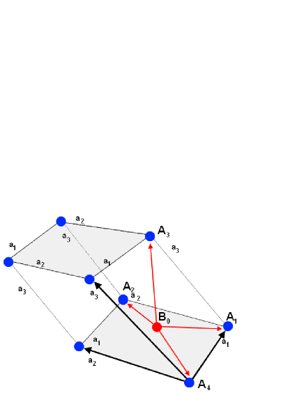
Figure 4: 3-dimensional projection of the real unit cell of hyperdiamond in the primitive frame. It is generated by the 4 vectors $\mathbf{a}_{1},\mathbf{a}_{2},\mathbf{a}_{3},$ $\mathbf{a}_{4}$ ( or up to scale factor by the 4 simple roots $\mathbf{\alpha}_{1},\mathbf{\alpha}_{2},\mathbf{\alpha}_{3},$ $\mathbf{\alpha}_{4}$ of $SU\left({\small 5}\right)$). Sites $A_{i}$ (resp $B_{i}$) belong to sublattice $\mathbb{A}$ (resp $\mathbb{B}$) of the hyperdiamond. B₀ has 5 nearest neighbors of A-type.

The first Brillouin zone of hyperdiamond is given by the unit cell in the momentum space generated by the $\mathbf{b}_{i}$’s; its hyper-volume is

$$\mathbf{b}_{1}\wedge\mathbf{b}_{2}\wedge\mathbf{b}_{3}\wedge\mathbf{b}_{4}=\frac{64\pi^{4}}{a^{4}}\det\left(\omega_{\mu}^{i}\right),$$ (86)

and is equal to $\frac{\left(2\pi\right)^{4}}{V_{uc}}$ with $V_{uc}$ the volume of the real cell given by (85). Notice that the 4 vectors $\mathbf{b}_{i}$ (or up to a scale factor $\mathbf{\omega}^{i}$) that generate the reciprocal space are dual to the $\mathbf{a}_{i}$ vectors (simple roots $\mathbf{\alpha}_{i}$); they obey

$$\mathbf{b}_{i}.\mathbf{a}_{j}=2\pi\delta_{ij}$$ , .

(87)

and give a nice group theoretical interpretation of the relation between the real and momentum spaces.

• More on hyperdiamond and $SU\left(5\right)$

Hyperdiamond $\mathbb{L}_{4}$ is a 4-dimensional lattice contained in $\mathbb{R}^{4}$; it can be thought of as made of the superposition of two 4-dimensional sublattices $\mathbb{A}$ and $\mathbb{B}$. Each site $\mathbf{r}_{n}$ in $\mathbb{A}$ has $5$ nearest neighbors $\left(\mathbf{r}_{n}+d\mathbf{e}_{i}\right)$ belonging to $\mathbb{B},$

$$\mathbf{r}_{n}\in\mathbb{A\rightarrow}\left\{\begin{array}[c]{c}\mathbf{r}_{n}+d\mathbf{e}_{1}\\ \mathbf{r}_{n}+d\mathbf{e}_{2}\\ \mathbf{r}_{n}+d\mathbf{e}_{3}\\ \mathbf{r}_{n}+d\mathbf{e}_{4}\\ \mathbf{r}_{n}+d\mathbf{e}_{5}\end{array}\right.\in\mathbb{B}$$

and 20 second nearest ones $\mathbf{r}_{n}+d\left(\mathbf{e}_{i}-\mathbf{e}_{j}\right)$ belonging to $\mathbb{A}$. The 5 vectors $\mathbf{e}_{i}$, giving the relative positions of the neighbors, obey the traceless property

$$\mathbf{e}_{1}+\mathbf{e}_{2}+\mathbf{e}_{3}+\mathbf{e}_{4}+\mathbf{e}_{5}=0,$$ (88)

capturing the hidden $SU\left(5\right)$ symmetry of the hyperdiamond.

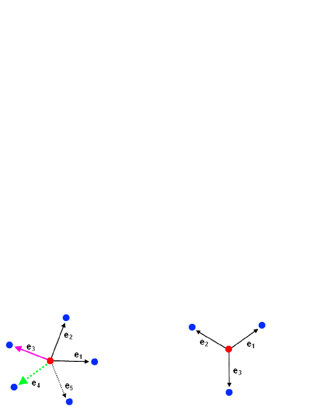
Figure 5: On left the 5 first nearest neighbors in the 4D hyperdiamond with the property $\mathbf{e}_{1}+\mathbf{e}_{2}+\mathbf{e}_{3}+\mathbf{e}_{4}+\mathbf{e}_{5}=0$. On right, the 3 first nearest in 2D graphene with $\mathbf{e}_{1}+\mathbf{e}_{2}+\mathbf{e}_{3}=0$.

To parameterize the site positions $\mathbf{r}_{n}$ of $\mathbb{L}_{4}$, it is useful to use $\mathbf{e}_{1}\mathbf{,}$ $\mathbf{e}_{2}\mathbf{,}$ $\mathbf{e}_{3}\mathbf{,}$ $\mathbf{e}_{4}$ to generate vectors in hyperdiamond. These 4 basis vectors $\mathbf{e}_{i}$ have the following intersection matrix

$$\mathbf{e}_{i}.\mathbf{e}_{j}=\left(\begin{array}[c]{cccc}1&-\frac{1}{4}&0&0\\ -\frac{1}{4}&1&-\frac{1}{4}&0\\ 0&-\frac{1}{4}&1&-\frac{1}{4}\\ 0&0&-\frac{1}{4}&1\end{array}\right)$$ ,

(89)

and can be realized as

$$\mathbf{e}_{1}^{\mu}$$

           (90)

These 5 vectors $\mathbf{e}_{1}\mathbf{,}$ $\mathbf{e}_{2}\mathbf{,}$ $\mathbf{e}_{3}\mathbf{,}$ $\mathbf{e}_{4},$ $\mathbf{e}_{5}$ define the first nearest neighbors to $\left(0,0,0,0\right)$ as in fig 5; they satisfy the relations $\mathbf{e}_{i}.\mathbf{e}_{i}=1$ and $\mathbf{e}_{i}.\mathbf{e}_{j}=-\frac{1}{4}$ $\ \forall$ $i\neq j$ showing that they are distributed in a symmetric way as required by the hidden SU$\left(5\right)$ symmetry of $\mathbb{L}_{4}$. The 20 second nearest neighbors are given by

$$\mathbf{e}_{ij}=\mathbf{e}_{i}-\mathbf{e}_{j}$$ , ,

(91)

and are remarkably generated by the 4 basis vectors

$$\mathbf{\alpha}_{1}=\frac{2\sqrt{5}}{5}\left(\mathbf{e}_{1}-\mathbf{e}_{2}\right)$$ ,

,

         (92)

By using (90), we have

$$\mathbf{\alpha}_{1}=\left(0,1,1,0\right)$$ ,

,

         (93)

from which we learn that $\mathbf{\alpha}_{i}^{2}=2$ and $\det\left(\mathbf{\alpha}_{1},\mathbf{\alpha}_{2},\mathbf{\alpha}_{3},\mathbf{\alpha}_{4}\right)=\sqrt{5}$. We also have the intersection matrix $C_{ij}=\mathbf{\alpha}_{i}.\mathbf{\alpha}_{j}$

$$C_{ij}=\left(\begin{array}[c]{cccc}2&-1&0&0\\ -1&2&-1&0\\ 0&-1&2&-1\\ 0&0&-1&2\end{array}\right)$$ ,

(94)

indicating that the $\mathbf{\alpha}_{i}$’s are nothing but the 4 simple roots of $SU\left(5\right)$ and $C_{ij}$ the corresponding Cartan matrix with inverse $G^{ij}$ as

$$G^{ij}=\left(\begin{array}[c]{cccc}\frac{4}{5}&\frac{3}{5}&\frac{2}{5}&\frac{1}{5}\\ \frac{3}{5}&\frac{6}{5}&\frac{4}{5}&\frac{2}{5}\\ \frac{2}{5}&\frac{4}{5}&\frac{6}{5}&\frac{3}{5}\\ \frac{1}{5}&\frac{2}{5}&\frac{3}{5}&\frac{4}{5}\end{array}\right)$$ .

(95)

This matrix $G^{ij}$ is just the intersection matrix of the fundamental weight vectors $\mathbf{\omega}^{i}$ of SU$\left(5\right)$

$$G^{ij}=\mathbf{\omega}^{i}.\mathbf{\omega}^{j}$$ ,

(96)

with

$$\left\|\mathbf{\omega}^{1}\right\|^{2}=\left\|\mathbf{\omega}^{4}\right\|^{2}=\frac{4}{5}$$ , .

(97)

The $\mathbf{\omega}^{i}$’s span the momentum space of the hyperdiamond; their components in the canonical basis are

$$\mathbf{\omega}^{1}=\left(\frac{1}{2},\frac{1}{2},\frac{1}{2},\frac{\sqrt{5}}{10}\right)$$ ,

,

(98)

with $\det\left(\mathbf{\omega}^{1},\mathbf{\omega}^{2},\mathbf{\omega}^{3},\mathbf{\omega}^{4}\right)=-\frac{1}{5}\sqrt{5}$. Therefore, generic positions $\mathbf{r}$ of $\mathbb{R}^{4}$ and generic wave vectors $\mathbf{k}$ of the 4-dimensional momentum space decompose as follows,

$$\mathbf{r}={\displaystyle\sum\limits_{i=1}^{4}}x^{i}\mathbf{\alpha}_{i}$$ ,

,

(99)

With these tools, we can determine several features on the crystallographic structure of the hyperdiamond; for instance the volume $V_{uc}$ of the real unit cell is $V_{uc}=\frac{a^{4}}{4}\sqrt{5}$; and the volume of first Brillouin zone $V_{BZ}$ reads as $V_{BZ}=\frac{64\pi^{4}}{5a^{4}}\sqrt{5}$. Recall also that the SU$\left(5\right)$ Lie algebra has 10 positive roots and 10 negative ones (opposites); the positive ones consists of the 4 above simple and the 6 following

$$\mathbf{\alpha}_{1}+\mathbf{\alpha}_{2},$$

(100)

Notice moreover that being also 4-dimensional vectors, the $\mathbf{\omega}^{i}$’s may be decomposed as well like a sum over simple roots

$$\mathbf{\omega}_{1}=\frac{4}{5}\mathbf{\alpha}_{1}+\frac{3}{5}\mathbf{\alpha}_{2}+\frac{2}{5}\mathbf{\alpha}_{3}+\frac{1}{5}\mathbf{\alpha}_{4}\$$

         (101)

offering a unified way to parameterize the hyperdiamond $\mathbb{L}_{4}$; its sublattices $\mathbb{A}$ and $\mathbb{B}$ and their reciprocal spaces.

IV.2 Supercell compactification

First we study supercell $C_{\text{supercell}}$ compactification in hyperdiamond; then we move to deal with the boundary conditions of fields on supercell $C_{\text{supercell}}\equiv SC_{4}$.

IV.2.1 p-cycles in supercell and 4-torus homology

The supercell $SC_{4}$ in hyperdiamond is 4-dimensional extensions of fig 3; and is described by a hyper-parallelogram $\mathcal{P}_{4}$ with periodic boundary conditions. Positions in supercell are parameterized by the vectors $\mathbf{r=}\sum_{i}x^{i}\frac{\sqrt{2}}{2}\mathbf{\alpha}_{i}$ with the real coordinates $x^{i}=\left(x,y,z,\tau\right)$ compactified as

$$0\leq x^{i}<l_{i}$$ , , .

     (102)

The 4D-parallelogram $\mathcal{P}_{4}$ is a real compact 4-cycle with the homology class of a 4-torus $\mathbb{T}^{4}$; it has the following features:

• $\mathcal{P}_{4}$ has 4 basis divisors $\Delta_{i}$ and 4 dual 1-cycles $E_{i}$ associated with the hyper-planes $x^{i}=0$ in $\mathcal{P}_{4}$. These are:

  3-cycles duals $$=$$ 1-cycles

      

  where $\Delta_{i}$ have the homology of a 3-torus $\mathbb{T}^{3}$ and $E_{i}$ of a circle $\mathbb{S}^{1}$. Positions in $E_{1}$ and in $\Delta_{1}$ are given by the vectors

  $$E_{1}$$ :

  :

  (103)

  with the corresponding volume forms:

  $$E_{1}$$ :

  :

  (104)

  Similar relations can be written down for the others $E_{i}$’s and $\Delta_{i}$’s.

• $\mathcal{P}_{4}$ has also six 2-cycles $C_{ij}$ and six dual ones $\tilde{C}_{ij}$ given by 2D-parallelograms.

  2-cycles dual 2-cycles

  $$x=y=0$$

  (105)

  These 2-cycles have the homology of 2-torii $\mathbb{T}^{2}$; they will be used later on to compute the fluxes of the background field components going through $C_{ij}$. These 2-cycles are needed for the derivation of the topological index of the Dirac operator. Positions in these cycles are as

  $$C_{12}$$ :

  :

  (106)

  with volume forms like

  $$C_{12}$$ :

  :

  (107)

  Similar relations can be written down for the others.

• the 4D-parallelogram $\mathcal{P}_{4}$ has $2^{4}$ vertices, they read in the P-frame as follows

  $$\left(l_{1}\epsilon_{1},\text{ }l_{2}\epsilon_{2},\text{ }l_{3}\epsilon_{3},l_{4}\epsilon_{4}\right)$$ , .

  (108)

  with the $l_{i}$’s as in (102).

Notice that as a 4-cycle, the 4D-parallelogram $\mathcal{P}_{4}$ and its p-cycles are generated by the 1-cycle basis $E_{1}$, $E_{2}$, $E_{3}$, $E_{4}$. Notice also that hyperdiamond sites in $SC_{4}$ are given by discrete position vectors $\mathbf{r}_{\mathbf{n}}$ belonging to two classes

$$\left\{\mathbf{r}_{\mathbf{n}}^{\mathbb{A}}\begin{tabular}[c]{l}\\ \end{tabular}\right\}\cup\left\{\mathbf{r}_{\mathbf{n}}^{\mathbb{B}}\begin{tabular}[c]{l}\\ \end{tabular}\right\}$$

respectively associated with the sublattice $\mathbb{A}$ and the sublattice $\mathbb{B}$. Sites in $\mathbb{A}$ are given by the integer vectors

$$\mathbf{r}_{\mathbf{n}}^{\mathbb{A}}=n_{1}\mathbf{a}_{1}+n_{2}\mathbf{a}_{2}+n_{3}\mathbf{a}_{3}+n_{4}\mathbf{a}_{4}$$ ,

(109)

with $\mathbf{a}_{i}$ as in (82) and $\mathbf{n}=\left(n_{1},n_{2},n_{3},n_{4}\right)$. The sites of the sublattice $\mathbb{B}$ are given by the globally shifted ones,

$$\mathbf{r}_{\mathbf{n}}^{\mathbb{B}}$$

(110)

with shift vector $\mathbf{s}=\mathbf{r}_{n}^{\mathbb{B}}-\mathbf{r}_{n}^{\mathbb{A}}$ given by

$$\mathbf{s}$$

(111)

By substituting the vectors $\mathbf{a}_{i}$ by their expressions (93), we obtain

$$\mathbf{s}=\left(\begin{array}[c]{c}0\\ 0\\ 0\\ d\end{array}\right)$$ (112)

Notice also that the total number of sites in the supercell (102) is $2N_{1}N_{2}N_{3}N_{4}$; half of them belong to the sublattice $\mathbb{A}$ and the other half to $\mathbb{B}$.

IV.2.2 Boundary conditions

To recover the hyperdiamond lattice from a given supercell, one uses periodic boundary conditions on its borders as

$$\mathbf{r}$$ ,

,

(113)

or equivalently

$$\mathbf{r}\equiv\mathbf{r}+l_{i}\frac{\sqrt{2}}{2}\mathbf{\alpha}_{i}.$$ (114)

To get the right spectrum of the Dirac operator, one has also to worry about the boundary conditions on the gauge field $\mathcal{A}_{\mu}\left(\mathbf{r}\right)$ and the fermionic waves $\Psi\left(\mathbf{r}\right)$ living on supercell. Generally these boundary conditions close up to a gauge transformation as follows

F$$\left(\mathbf{r}+\frac{l_{i}\sqrt{2}}{2}\mathbf{\alpha}_{i}\right)$$ F

     (115)

where F stands for $\mathcal{A}_{\mu}$, $\Psi$ and where $\Omega_{i}$ some particular gauge transformation along the $\mathbf{\alpha}_{i}$- direction. To deal with the conditions (115), we extend the trick of Smit and Vink B2 that we have developed in section 3 by taking the gauge fields as

$$\mathcal{A}_{x}\left(\mathbf{r}\right)=0$$ ,

,

     (116)

with no dependence in the $y$ nor $\tau$ variables. This particular gauge choice allows amongst others the two following helpful features:
(i) it permits to use gauge invariance $\mathcal{A}_{i}^{\Omega}\left(\mathbf{r}\right)=\mathcal{A}_{i}\left(\mathbf{r}\right)+\partial_{i}\lambda$ to ensure the periodicity of the components of the gauge potential. This leads to a strong constraint on the y- and $\tau$- dependence into the gauge parameter $\lambda$ which are no longer arbitrary since they have to take the form

$$\lambda\left(\mathbf{r}\right)=\mathcal{B}l_{1}y+\mathcal{E}l_{3}\tau+\varphi\left(x,z\right),\qquad\Omega\left(\mathbf{r}\right)=e^{i\lambda\left(\mathbf{r}\right)}$$ (117)

with some integration function $\varphi\left(x,z\right)$ that we drop out below as it is not of great importance for the following analysis. Moreover periodicity of the gauge group element on supercell which has to obey $\Omega\left(\mathbf{r}+\frac{l_{i}\sqrt{2}}{2}\mathbf{\alpha}_{i}\right)=\Omega\left(\mathbf{r}\right)$ leads to the quantization of the background fields as follows

$$\mathcal{B}l_{1}l_{2}$$ ,

,

(118)

(ii) it permits also to put the boundary condition on the fermionic waves into two classes: the two trivial ones

$$\Psi\left(x,y+l_{2},z,\tau\right)$$

     (119)

easy to deal with; and the two less trivial ones

$$\Psi\left(x+l_{1},y,z,\tau\right)$$

(120)

where $\Omega_{1}$ and $\Omega_{3}$ are particular gauge transformations to be given later on.
Eq(119) allows to expand $\Psi\left(x,y,z,\tau\right)$ in Fourier modes as follows

$$\Psi\left(x,y,z,\tau\right)={\displaystyle\sum\limits_{r\in\mathbb{Z}}}e^{i\frac{2\pi r}{L_{2}}y}{\displaystyle\sum\limits_{s\in\mathbb{Z}}}e^{i\frac{2\pi s}{l_{4}}\tau}\text{ }\tilde{\Psi}_{r,s}\left(x,z\right)$$ (121)

restricting the problem of computing wave functions to looking for the Fourier modes $\tilde{\Psi}_{r,s}\left(x,z\right)$ whose dependence in x and z variables of $\tilde{\Psi}_{r,s}\left(x,z\right)$ can be obtained by solving the Dirac equation that we study below.

V Spectrum of Dirac operator

Here, we compute the spectrum of the fermions on hyperdiamond. First we consider the case of the continuum limit (unit cell). This is interesting to compare with the case of lattice fermions using supercell compactification to be considered later on.

V.1 Dirac equation coupled to $\mathcal{F}_{\mu\nu}$: continuum case

The Dirac equation describing the dynamics of four component Dirac fermions $\Psi_{\alpha}^{a}\left(\mathbf{x}\right)$, with $SU_{C}\left(3\right)$ color symmetry in presence of background vector potentials $\mathcal{A}_{\mu}^{G}\left(\mathbf{x}\right)$, is given by,

$$\sum_{\mu=1}^{4}\sum_{\beta=1}^{4}\sum_{b=1}^{3}i\left(\gamma^{\mu}\right)_{\alpha}^{\beta}\left[\delta_{ab}\partial_{\mu}-i\left(\mathcal{A}_{\mu}^{G}\right)_{ab}\right]\Psi_{\beta}^{b}=\epsilon\Psi_{\alpha}^{b}$$ (122)

where

$$\Psi_{\alpha}^{a}=\left(\begin{array}[c]{c}\Psi_{\alpha}^{1}\\ \Psi_{\alpha}^{2}\\ \Psi_{\alpha}^{3}\end{array}\right),$$

and

$$\Psi_{\alpha}^{a}=\left(\begin{array}[c]{c}\Psi_{L}^{a}\\ \Psi_{R}^{a}\end{array}\right),$$

  

and where $\mathcal{A}_{\mu}^{G}=\mathcal{A}_{\mu}^{U_{em}\left(1\right)}+\mathcal{A}_{\mu}^{SU_{c}\left(3\right)}$ with

$$\mathcal{A}_{\mu}^{U_{em}\left(1\right)}=\mathcal{A}_{\mu}^{em}Q_{em}\text{, \qquad}\mathcal{A}_{\mu}^{SU_{c}\left(3\right)}={\displaystyle\sum\limits_{I=1}^{8}}\mathcal{A}_{\mu}^{I}\mathcal{T}_{I}$$ (123)

with the $3\times 3$ matrices $\mathcal{T}_{I}$ standing for the generators of $SU_{c}\left(3\right)$. Below, we focus on the particular case where

$$\mathcal{A}_{\mu}^{U_{em}\left(1\right)}\neq 0$$ , ,

(124)

but keep in mind that such analysis can be straightforwardly extended to include the other abelian components $\mathcal{A}_{\mu}^{SU_{c}\left(3\right)}\neq 0$ leading to a non zero uniform field strength $\mathcal{F}_{\mu\nu}^{SU_{c}\left(3\right)}$ along the Cartan directions in the $SU_{C}\left(3\right)$ Lie algebra. Notice that in (122) the number $\epsilon$ captures deformations of the energy spectrum around the Dirac point where live zero modes of QCD₄ fermions on lattice. Notice also that here we have ignored the flavor symmetry which is associated with the zero modes in the tight binding description of QCD on lattice; for details on implementation of flavor symmetry in the case minimally doubled fermions see PSM ; 5A .

• Dirac equation in continuum

By setting $A_{\mu}^{SU_{c}\left(3\right)}=0$ in eq(122), the Dirac equation in the canonical frame of the euclidian space $\mathbb{R}^{4}$ reduces to its usual form,

$$i\gamma^{\mu}\left(\partial_{\mu}-iA_{\mu}\right)\Psi=\epsilon\Psi.$$ (125)

In this equation, the $4\times 4$ matrices $\gamma^{\mu}$ are euclidian Dirac matrices obeying the usual 4D Clifford algebra $\gamma^{\mu}\gamma^{\nu}+\gamma^{\nu}\gamma^{\mu}=2\delta^{\mu\nu}I_{4}$ with $I_{4}$ the $4\times 4$ identity matrix. These $\gamma^{\mu}$ matrices can be built by using the Pauli ones $\tau^{i}$ and $\sigma^{i}$ of the group product $SU_{L}\left(2\right)\times SU_{R}\left(2\right)\simeq SO\left(4\right)$,

$$\varrho^{1}=\left(\begin{array}[c]{cc}0&1\\ 1&0\end{array}\right),$$

(126)

with $\varrho^{i}$ standing for both $\tau^{i}$ and $\sigma^{i}$. The $\varrho^{1}$, $\varrho^{2}$ satisfy the 2D Clifford algebra $\varrho^{i}\varrho^{j}+\varrho^{j}\varrho^{i}=2\delta^{ij}I_{2}$ and the $SU\left(2\right)$ symmetry bracket $\left[\varrho^{1},\varrho^{2}\right]=2i\varrho^{3}$. We have

$$\gamma^{i}=\tau^{2}\otimes\sigma^{i}$$ ,

,

       (127)

with $\tau^{4}$, $\sigma^{4}=I_{2}\equiv I$ and $\gamma^{5}=\gamma^{1}\gamma^{2}\gamma^{3}\gamma^{4}$. More explicitly

$$\gamma^{k}{\small=}\left(\begin{array}[c]{cc}{\small 0}&{\small-i\sigma}^{k}\\ {\small i\sigma}^{k}&{\small 0}\end{array}\right)$$,

(128)

and

$$\gamma^{5}=\left(\begin{array}[c]{cccc}1&0&0&0\\ 0&1&0&0\\ 0&0&-1&0\\ 0&0&0&-1\end{array}\right)$$ ,

(129)

The commutators $\gamma^{\left[\mu\nu\right]}$ give precisely the 6 generators of the spinorial representation of the $SO\left(4\right)$ symmetry,

$$\gamma^{i}\gamma^{j}-\gamma^{j}\gamma^{i}$$ ,

,

(130)

where $\varepsilon^{ijk}$ is the completely antisymmetric 3D Levi-Civita tensor.
The Dirac operator (125) involves also the gauge potential $A_{\mu}$ defined up to the gauge symmetry transformations

$$\Psi=e^{-i\lambda}\Psi$$ , ,

      

with $\lambda\left(\mathbf{x}\right)$ arbitrary gauge parameter. Since the background field strength $F_{\mu\nu}=\partial_{\mu}A_{\nu}-\partial_{\nu}A_{\mu}$ is a constant, the gauge potential $A_{\mu}$ reads as follows,

$$A_{\mu}=\frac{1}{2}F_{\mu\nu}x^{\nu}$$ ,

       (131)

Notice that generally $F_{\mu\nu}$ has six real degrees of freedom, 3 magnetic $B_{i}$ and 3 electric $E_{i}$:

$$F_{\mu\nu}=\left(\begin{array}[c]{cccc}0&+B_{3}&-B_{2}&+E_{1}\\ -B_{3}&0&+B_{1}&+E_{2}\\ +B_{2}&-B_{1}&0&+E_{3}\\ -E_{1}&-E_{2}&-E_{3}&0\end{array}\right).$$ (132)

• Choice of the background fields

Below we will think about this $F_{\mu\nu}$ as a sub-matrix of the following $5\times 5$ antisymmetric one,

$$F_{MN}=\left(\begin{array}[c]{cc}F_{\mu\nu}&F_{\mu 5}\\ F_{5\nu}&0\end{array}\right),$$ (133)

where now the $F_{\mu 5}$’s are the 4 components of the electric field in $5D$; and $F_{\mu\nu}$ are the 6 components of the magnetic tensor. We also make the two following useful choices:
(i) we restrict the matrix $F_{\mu\nu}$ to the particular case,

$$F_{\mu\nu}=\left(\begin{array}[c]{cccc}0&-B&0&0\\ +B&0&0&0\\ 0&0&0&-E\\ 0&0&+E&0\end{array}\right)$$ (134)

allowing exact computations due to the decoupling of the left and right sectors of fermions. Using the antisymmetric tensor $\varepsilon_{\mu\nu\rho\sigma}$, we have

$$F_{\mu\nu}=B\varepsilon_{\mu\nu 34}+E\varepsilon_{12\mu\nu}.$$ (135)

(ii) To deal with the gauge field, we can either use the symmetric choice

$$A_{1}=\frac{B}{2}y,$$

     (136)

or the Smit-Vink method

$$A_{1}=0,$$

     (137)

In the next sub-subsection, we use the first choice as it allows to take advantage of the symmetric role played by the components fields to solve the Dirac equation in the continuum. Later on, we use the second choice to study the Dirac operator of fermion on supercell; the gauge (137) is convenient for the study the degeneracy of the zero modes of the Dirac operator and its topological index.

V.2 Spectrum in the gauge (136)

To get the spectrum of the Dirac operator (125), notice that the 4 gauge covariant derivatives $D_{1},$ $D_{2},$ $D_{3},$ $D_{4}$ satisfy the generic commutation relations

$$\left[D_{\mu},D_{\nu}\right]=-iF_{\mu\nu},$$ (138)

but because of the choice (134) of the background fields, they reduce to,

$$\left[D_{1},D_{2}\right]$$ ,

,

   (139)

and all others vanishing.

V.2.1 Deriving the wave functions

The fermionic wave functions solving the Dirac equation are given by representations of the algebra (139). By using (136), the four covariant derivatives organize in $2+2$ capturing a complex structure as follows,

(142)

In getting these relations, we have used the explicit expressions $D_{1}=\partial_{1}-i\frac{QB}{2c}y$, $D_{2}=\partial_{2}+i\frac{QB}{2c}x$ together with similar relations for $D_{3}$, $D_{4}$; and we have set

$$u=x+iy$$ , ,

, .

     (143)

The representations of eqs(139) depends on the sign of $B$ and $E$. Setting

$$i\left(D_{1}-iD_{2}\right)=A^{-}\sqrt{2\left|B\right|}$$ , ,

, ,

     (144)

the commutation relations (139) read also as

$$\left[A^{-},A^{+}\right]=\frac{B}{\left|B\right|}I$$ , ,

, ;

     (145)

These relations (145) show that the Dirac fermion in the background field $F_{\mu\nu}$ (134) describe a priori 2 quantum harmonic oscillators with oscillation frequencies

$$\mathrm{\nu}=\sqrt{2\left|B\right|}\qquad,\qquad\mathrm{\nu}^{\prime}=\sqrt{2\left|B\right|}.$$ (146)

The operators $A^{+}A^{-}$ and $C^{+}C^{-}$ , which a priori give the number of energy excitations in $\mathrm{\nu}$ and $\mathrm{\nu}^{\prime}$ units respectively, read in terms of the gauge covariant derivatives as follows

$$2\left|B\right|A^{+}A^{-}$$ =

= ,

(147)

and similarly

$$2\left|E\right|C^{+}C^{-}$$ =

= .

(148)

Using the expression of the matrices $\gamma^{\mu}$, we can write this matrix operator $H_{\alpha\beta}=i\gamma_{\alpha\beta}^{\mu}D_{\mu}$ in terms of the ”creation” operators $A^{+},$ $C^{+}$ and the ”annihilation” ones $A^{-},$ $C^{-}$ as follows:

$$H_{\alpha\beta} =\frac{1}{i}\left(\begin{array}[c]{cccc}0&0&-\mathrm{\nu}^{\prime}C^{+}&-\mathrm{\nu}A^{-}\\ 0&0&-\mathrm{\nu}A^{+}&\mathrm{\nu}^{\prime}C^{-}\\ \mathrm{\nu}^{\prime}C^{-}&\mathrm{\nu}A^{-}&0&0\\ \mathrm{\nu}A^{+}&-\mathrm{\nu}^{\prime}C^{+}&0&0\end{array}\right),$$ (153)

with $H^{\dagger}=H$. Moreover, using the commutation properties $C^{+}A^{\pm}=A^{\pm}C^{+}$ and $C^{-}A^{\pm}=A^{\pm}C^{-}$, the squared hamiltonian $H^{2}$ reads as follows,

$$\left(\begin{array}[c]{cccc}{\small\nu}^{{\small 2}}{\small A}^{-}{\small A}^{+}{\small+\nu}^{\prime{\small 2}}{\small C}^{+}{\small C}^{-}&0&0&0\\ 0&{\small\nu}^{{\small 2}}{\small A}^{+}{\small A}^{-}{\small+\nu^{\prime 2}C}^{-}{\small C}^{+}&0&0\\ 0&0&{\small\nu}^{{\small 2}}{\small A}^{-}{\small A}^{+}{\small+\nu^{\prime 2}C}^{-}{\small C}^{+}&0\\ 0&0&0&{\small\nu}^{{\small 2}}{\small A}^{+}{\small A}^{-}{\small+\nu^{\prime 2}C}^{+}{\small C}^{-}\end{array}\right)$$

and, by using $\Psi=\left(\mathrm{\psi}_{a},\mathrm{\bar{\xi}}_{\dot{a}}\right)$, leads to

$$\mathcal{O\mathcal{O}}^{\dagger}\left(\begin{array}[c]{c}\psi_{1}\\ \psi_{2}\end{array}\right)$$ ,

,

     (154)

with

(162)

showing that the two Weyl spinors $\psi_{a}$ and $\bar{\xi}_{\dot{a}}$ can be treated separately. Putting the expression of $\mathcal{OO}^{\dagger}$ and $\mathcal{O}^{\dagger}\mathcal{O}$ back into eq(154), we obtain

$$\left(\mathrm{\nu}^{\prime 2}C^{+}C^{-}+\mathrm{\nu}^{2}A^{-}A^{+}\right)\psi_{1}$$ ,

,

,

.

(163)

The solutions of these equations depend on the sign of the background fields $B$ and $E$. In the case $\frac{B}{\left|B\right|}>0$, $\frac{E}{\left|E\right|}>0$, we have:

$$\left(\begin{array}[c]{c}\psi_{1}\\ \psi_{2}\\ \bar{\xi}_{1}\\ \bar{\xi}_{2}\end{array}\right)=\left(\begin{array}[c]{c}\mathbf{\Theta}_{n-1,\text{ }m}\text{ \ \ }\\ \Theta_{n,\text{ }m-1}\text{ \ }\\ \Theta_{n-1,\text{ }m-1}\\ \Theta_{n,\text{ }m}\text{ \ \ \ \ }\end{array}\right)$$ (164)

with

$$\Theta_{n,m}\left(u,\bar{u},v,\bar{v}\right)=\theta_{n}\left(u,\bar{u}\right)\times\theta_{m}^{\prime}\left(v,\bar{v}\right),\qquad n,m\geq 0,$$ (165)

and

$$A^{-}\times\theta_{0}\left(u,\bar{u}\right)=\left(\frac{2\partial}{\partial u}+\frac{QB}{2c}\bar{u}\right)\theta_{0}\left(u,\bar{u}\right)=0$$

(166)

solved as follows

$$\theta_{0}\left(u,\bar{u}\right)=\mathcal{N}_{0}\left(\bar{u}\right)e^{-\frac{QB}{4}u\bar{u}}$$ , ,

     (167)

where the complex functions $\mathcal{N}_{0}\left(\bar{u}\right)$ and $\mathcal{N}_{0}^{\prime}\left(\bar{v}\right)$ are anti-holomorphic functions. The excited waves functions $\theta_{n}\left(u,\bar{u}\right)$ and $\theta_{m}^{\prime}\left(v,\bar{v}\right)$ are obtained by applying the creation operators.

$$\theta_{n}\left(u,\bar{u}\right)$$ ,

.

     (168)

V.2.2 Zero modes and topological index

The zero modes of the Dirac operator depend on the sign of the background fields $B$ and $E$ since the algebra of the commutation relations (145) depend on $\frac{B}{\left|B\right|}$ and $\frac{E}{\left|E\right|}$ as given below:

$$\left[A^{-},A^{+}\right]=\frac{B}{\left|B\right|}I$$ , .

(169)

We have the 4 following possibilities:

(a) Case $\frac{B}{\left|B\right|}>0$, $\frac{E}{\left|E\right|}>0$
In this situation, the $A^{+},$ $C^{+}$ are creation operators and $A^{-},$ $C^{-}$ annihilation ones. So the zero mode is given by

$$\Psi_{\epsilon=0}=\left(\begin{array}[c]{c}0\text{\ }\\ 0\\ 0\\ \mathbf{\Theta}_{0,0}\end{array}\right)$$ (170)

with the chirality property

$$\left(\sigma^{3}\otimes\tau^{3}\right)\Psi_{\epsilon=0}$$

(171)

and by setting $Tr\left(\bar{\Psi}_{\epsilon=0}\Psi_{\varepsilon=0}\right)=1$, we have

$$Tr\left[\bar{\Psi}_{\epsilon=0}\left(\sigma^{3}\otimes\tau^{3}\right)\Psi_{\varepsilon=0}\right]$$

(172)

(b) Case $\frac{B}{\left|B\right|}<0$, $\frac{E}{\left|E\right|}<0$
In this case $A^{+},$ $C^{+}$ are annihilation operators and $A^{-},$ $C^{-}$ creation ones so that the zero mode is

$$\Psi_{\epsilon=0}$$ ,

(173)

and

$$\left(\sigma^{3}\otimes\tau^{3}\right)\Psi_{\epsilon=0}$$

(174)

as well as

$$Tr\left[\bar{\Psi}_{\epsilon=0}\left(\sigma^{3}\otimes\tau^{3}\right)\Psi_{\varepsilon=0}\right]$$

(175)

(c) Case $\frac{B}{\left|B\right|}>0$, $\frac{E}{\left|E\right|}<0$
Here $A^{+},$ $C^{-}$ are creation operators and $A^{-},$ $C^{-}$ annihilations. The zero mode is given by

$$\Psi_{\epsilon=0}=\left(\begin{array}[c]{c}0\text{\ }\\ 0\\ \mathbf{\Theta}_{0,0}\\ 0\end{array}\right)$$ (176)

with

$$\left(\sigma^{3}\otimes\tau^{3}\right)\Psi_{\epsilon=0}$$

(177)

and

$$Tr\left[\bar{\Psi}_{\epsilon=0}\left(\sigma^{3}\otimes\tau^{3}\right)\Psi_{\varepsilon=0}\right]$$

(178)

(d) Case $\frac{B}{\left|B\right|}<0$, $\frac{E}{\left|E\right|}>0$
In this case, the zero mode reads as

$$\Psi_{\epsilon=0}=\left(\begin{array}[c]{c}0\text{\ }\\ \mathbf{\Theta}_{0,0}\\ 0\\ 0\end{array}\right)$$ (179)

with

$$\left(\sigma^{3}\otimes\tau^{3}\right)\Psi_{\epsilon=0}$$

(180)

and

$$Tr\left[\bar{\Psi}_{\epsilon=0}\left(\sigma^{3}\otimes\tau^{3}\right)\Psi_{\varepsilon=0}\right]$$

(181)

From the above analysis on the chirality of zero modes, it follows that the chirality operator that satisfies the Atiyah-Singer theorem is $\sigma^{3}\otimes\tau^{3}$ since

$$Tr\left[\bar{\Psi}_{\epsilon=0}\left(\sigma^{3}\otimes\tau^{3}\right)\Psi_{\varepsilon=0}\right]$$

(182)

This feature can be explained as due to the factorization of the $SO\left(4\right)$ symmetry of $\mathbb{R}^{4}$ in terms of the product of $SU_{L}\left(2\right)\times SU_{R}\left(2\right)$. The relation that involves $\gamma^{5}$ reads as $Tr\left[\bar{\Psi}_{\epsilon=0}\gamma^{5}\Psi_{\varepsilon=0}\right]=\frac{E}{\left|E\right|}$.

VI Solving Dirac equation on supercell

To study the spectrum of the Dirac equation in the supercell compactification of the hyperdiamond, we extend the result of sub-section 5.2 concerning the continuum to the case of the 4D lattice. There, we have used the canonical frame of $\mathbb{R}^{4}$ with the local coordinates $X^{\mu}=\left(X,Y,Z,T\right)$; which will be used also in the case of lattice.
In the C-frame, the 4 gauge covariant derivatives $D_{\mu}=$ $\left(D_{1},D_{2},D_{3},D_{4}\right)$ satisfy the usual commutation relations giving the components of the U$\left(1\right)$ gauge curvature

$$\left[D_{\mu},D_{\nu}\right]=-iF_{\mu\nu}.$$ (183)

By choosing the background fields as in (134), these commutation relations factorize into two decoupled Heisenberg algebras as follows,

$$\left[D_{1},D_{2}\right]=iB$$ ,

,

(184)

To work out explicit solutions of these equations, one may used either the potential vector (136) or (137). In this section, we use eq(137) leading to the following gauge covariant derivatives $D_{\mu}=\frac{\partial}{\partial X^{\mu}}-iA_{\mu}$

$$D_{1}=\frac{\partial}{\partial X}$$ ,

,

       (185)

This choice breaks the symmetric role played by the variables $\left(X,Y\right)$ and $\left(Z,T\right)$; but is suitable to deal with the boundary conditions of the fields on supercell.
Notice that eqs(183) and (185) can be also expressed in the P- frame with positions as $x^{i}=\left(x,y,z,\tau\right)$. The passage between C- and P- frames is given by the transformations

$$X^{\mu}=\alpha_{i}^{\mu}x^{i}$$ , ,

       (186)

Similar relations can be written down for the other the objects; for instance the potential vector $A_{\mu}$ and the gauge covariant derivatives $D_{\mu}$ in C-frame are related to their homologue $\mathcal{A}_{i}$ and $\mathcal{D}_{i}$ in the P-frame as

$$A_{\mu}=\omega_{\mu}^{i}\mathcal{A}_{i}$$ ,

,

(187)

VI.1 Computing the fluxes of background fields

The flux of the background fields through hyperdiamond supercell is a scalar quantity and is frame independent. This flux give the total topological charge inside the supercell $SC_{4}$; it controls the chirality of the ground state and allows to determine the topological index of the Dirac operator in the background fields $B$ and $E$.
To compute the flux, one can either use the C-frame or the P-frame; in fact it is frame independent. To see this property recall that in the C-frame the gauge curvature is given by $F_{\mu\nu}$ and in the P-frame is $\mathcal{F}_{ij}$:

$$\left[D_{\mu},D_{\nu}\right]=-iF_{\mu\nu}$$ , .

(188)

These two tensors are related as

$$\mathcal{F}_{ij}$$

     (189)

with

$$\mathbf{\alpha}_{i}\wedge\mathbf{\alpha}_{j}$$

(190)

The corresponding gauge invariant 2-form field strengths are then given by

$$\mathcal{F}$$

(191)

and are equal $\mathcal{F}=F$ since they are frame independent; thanks to $\alpha_{i}^{\mu}\omega_{\mu}^{j}=\delta_{i}^{j}$. Moreover, because of the choice

$$F_{\mu\nu}=B\varepsilon_{\mu\nu 34}+E\varepsilon_{12\mu\nu}$$ (192)

that we have used in this paper to work out explicit solutions of the Dirac equation, the 2-form $F$ reduces to the simple expression

$$F$$

     (193)

By using the coordinate change (186) to the P-frame, it can be also written as

$$F$$

(194)

where $F$ takes a general expression in the basis $dx^{i}\wedge dx^{j}$. With these relations at hand, we can compute the flux of the background fields through the various p-cycles of the supercell. We will do the calculations the C-frame.
The total topological charge $Q_{tot}$ of the background field within the supercell is given by the integration of the 4-form $F\wedge F$ over the supercell,

$$\frac{1}{\left(2\pi\right)^{2}}{\displaystyle\int\nolimits_{SC_{4}}}\frac{1}{2}F\wedge F=Q_{tot}$$ , ,

(195)

Substituting (193) back into (195), we obtain a quantization condition on the background fields given by

$$B\times E=\frac{\left(2\pi\right)^{2}}{L_{1}L_{2}L_{3}L_{4}}Q_{tot}$$ (196)

One can also compute the fluxes

$$\frac{1}{2\pi}\int_{C_{2}}F$$ (197)

of the field strength $F$ through the 2-cycles $C_{ij}\equiv C_{2}$ of the supercell; this gives extra quantization conditions. Because of the choice (134), non trivial fluxes are indeed given by the 2-cycles $C_{12}$ and $C_{34}$. Using the relation $F=dA$ to map the integration over the 2-cycles $C_{ij}$ to circulation around its boundaries $\partial C_{ij}$, we end with

$$\frac{1}{2\pi}{\displaystyle\int\nolimits_{C_{12}}}F$$

(198)

and

$$\frac{1}{2\pi}{\displaystyle\int\nolimits_{C_{34}}}F$$

(199)

giving two extra quantization conditions; one on the background field $B$ and the other on $E$. More precisely, we have:

$$B=\frac{2\pi}{L_{1}L_{2}}Q_{B}$$ ,

,

     (200)

Comparing (200) with (196) we get the following relation between the topological charges

$$Q_{tot}=Q_{B}Q_{E}.$$ (201)

VI.2 Dirac equation on 4D- supercell

The euclidian Dirac equation on supercell is given by the 4-dimensional extension of the Dirac equation on honeycomb lattice. In addition to periodic background potentials, this equation involves four component fermionic waves with boundary conditions described by the $SO\left(4\right)$ spinor $\Psi=\left(\psi_{a},\bar{\xi}_{\dot{a}}\right)$ that we want to determine below.

VI.2.1 The hamiltonian

The euclidian Dirac equation is

$$H\left(\begin{array}[c]{c}\psi_{a}\\ \bar{\xi}_{\dot{a}}\end{array}\right)=\epsilon\left(\begin{array}[c]{c}\psi_{a}\\ \bar{\xi}_{\dot{a}}\end{array}\right)$$ (202)

where the hamiltonian $H$ reads in the canonical frame as $H=\gamma^{\mu}D_{\mu}$ or equivalently in the P-frame

$$H=\gamma^{\mu}D_{\mu}=\gamma^{\mu}\omega_{\mu}^{i}\mathcal{D}_{i}=\Gamma^{i}\mathcal{D}_{i}$$ (203)

with $\Gamma^{i}=\gamma^{\mu}\omega_{\mu}^{i}$. The solution of (202) in continuum has been worked out in the previous section; below we want to extend these results to the lattice case where boundary conditions put strong constraints on the solutions. To that purpose, let us start by collecting useful tools. First the hamiltonian $H$ has the form

$$H=\left(\begin{array}[c]{cc}0&D\\ \bar{D}&0\end{array}\right)$$ ,

(204)

with

$$D=\left(\begin{array}[c]{cc}\sqrt{\left|E\right|}C^{-}&-i\sqrt{\left|B\right|}A^{-}\\ -i\sqrt{\left|B\right|}A^{+}&\sqrt{\left|E\right|}C^{+}\end{array}\right)$$ ,

(205)

and

$$\bar{D}=\left(\begin{array}[c]{cc}\sqrt{\left|E\right|}C^{+}&i\sqrt{\left|B\right|}A^{-}\\ i\sqrt{\left|B\right|}A^{+}&\sqrt{\left|E\right|}C^{-}\end{array}\right)$$ (206)

and where we have set

$$A^{-}=\frac{1}{\sqrt{\left|B\right|}}\left(D_{1}-iD_{2}\right)$$ ,

,

(207)

Second the operators $A^{\pm}$ and $C^{\pm}$ obey the commutation relations

$$\left[A^{-},A^{+}\right]$$ ,

,

     (208)

and all other vanishing. Notice that these commutation relations have a remarkable dependence on the sign of the background fields B and E. Third, the squared hamiltonian $H^{2}$ has the diagonal form

$$H^{2}=\left(\begin{array}[c]{cc}D\bar{D}&0\\ 0&\bar{D}D\end{array}\right)$$

with

$$D\bar{D}=\left(\begin{array}[c]{cc}\left|B\right|A^{-}A^{+}+\left|E\right|C^{-}C^{+}&0\\ 0&\left|B\right|A^{+}A^{-}+\left|E\right|C^{+}C^{-}\end{array}\right)$$ (209)

and

$$D\bar{D}=\left(\begin{array}[c]{cc}\left|B\right|A^{-}A^{+}+\left|E\right|C^{+}C^{-}&0\\ 0&\left|B\right|A^{+}A^{-}+\left|E\right|C^{-}C^{+}\end{array}\right)$$ (210)

involving the four possible quadratic combinations of $A^{\pm}$ and $C^{\pm}$ namely $A^{-}A^{+}$, $A^{+}A^{-}$, $C^{-}C^{+}$ and $C^{+}C^{-}$.

VI.2.2 The solutions and Index$\left(D\right)$

The solutions of (202) on supercell are representations of the algebra (208) that have to satisfy moreover the boundary conditions on the fields. These conditions are quite similar to those studied in the case of 2D honeycomb; so we omit here the lengthy technical details and just give the results.
There are 4 classes of solutions of (202) depending on the signs of $\frac{B}{\left|B\right|}$ and $\frac{E}{\left|E\right|}$. They are obtained as follows: First, expand the wave $\Psi\left(\mathbf{x}\right)$ on the periodic supercell in Fourier series as

$$\Psi\left(\mathbf{x}\right)$$

(211)

This expansion follows from the periodicity of $\Psi\left(\mathbf{x}\right)$ along the y- and $\tau$- axis. Second, solve the non trivial boundary conditions along the x- and z- axes by following the method used in the case of 2D honeycomb which lead to eqs(42-43). As in the present case we have to deal with the 2 variables x and z, we write the $\Psi_{l,q}\left(x,z\right)$ modes like

$$\Psi_{l,q}\left(x,z\right)=\Phi\left(\xi_{l},\zeta_{q}\right)$$ (212)

with

$$\xi_{l}=x+\frac{l}{Q_{B}}L_{1}$$ ,

(213)

The next step is to determine the function $\Phi\left(\xi,\zeta\right)$; this is a Dirac spinor which we set as

$$\Phi\left(\xi,\zeta\right)=\left(\begin{array}[c]{c}\phi\left(\xi,\zeta\right)\\ \varrho\left(\xi,\zeta\right)\\ \varphi\left(\xi,\zeta\right)\\ \chi\left(\xi,\zeta\right)\end{array}\right)$$ (214)

with components obeying the following coupled equations

$$\left(\left|B\right|A^{-}A^{+}+\left|E\right|C^{-}C^{+}\right)\phi$$

(215)

The operators $A^{\pm}$ and $C^{\pm}$ satisfy the algebra (208) and show that solutions for $\Phi\left(\xi,\zeta\right)$ depend on the sign of the background fields. These solutions are as follows:

• case $\frac{B}{\left|B\right|}>0$, $\frac{E}{\left|E\right|}>0$

In this case, which corresponds also to a positive topological charge $Q_{tot}$, the algebra (208) reads as follows

$$\left[A^{+},A^{-}\right]$$ ,

,

(216)

showing $A^{-}$, $C^{-}$ are creation operators and $A^{+}$, $C^{+}$ are annihilation ones. Using general results on quantum harmonic oscillators and the relations

$$\mathcal{N}_{A}=A^{-}A^{+}$$ ,

,

    

where $\mathcal{N}$ stands for the number operator, it is not difficult to see that the $\epsilon$ energies are discrete as

$$\epsilon_{{}_{n,m}}^{2}=n\left|B\right|+m\left|E\right|,\qquad n,m\in\mathbb{N}$$ (217)

and the corresponding wave functions $\Phi_{{}_{n,m}}$ are given by

$$\Phi_{{}_{{}_{n,m}}}\left(\xi,\zeta\right)=\left(\begin{array}[c]{c}\Theta_{{}_{n,m}}\text{ \ \ \ \ }\\ \Theta_{{}_{n-1,m-1}}\\ \Theta_{{}_{n,m-1}}\text{ \ \ }\\ \Theta_{{}_{n-1,m}}\text{ \ \ }\end{array}\right)$$ (218)

where

$$\Theta_{n,m}\left(\xi,\zeta\right)=\theta_{n}\left(\xi\right)\times\vartheta_{m}\left(\zeta\right)$$

and

$$\theta_{n}\left(\xi\right)$$ ,

,

(219)

with

$$\theta_{0}\left(\xi\right)=\mathcal{N}_{0}e^{-\frac{\left|B\right|}{2}\xi^{2}}$$ , .

(220)

Notice that because $\theta_{-1}\left(\xi\right)=\vartheta_{-1}\left(\zeta\right)=0,$ the ground state has only one component as

$$\Phi_{{}_{0,0}}=\left(\begin{array}[c]{c}\Theta_{{}_{0,0}}\\ 0\\ 0\\ 0\end{array}\right).$$ (221)

Moreover since the degeneracy of $\theta_{0}$ and $\vartheta_{0}$ are respectively $\left|Q_{B}\right|$ and $\left|Q_{E}\right|$; it follows that the degree of degeneracy of $\Phi_{0,0}$ is precisely the total topological charge

$$\left|Q_{B}Q_{E}\right|=\left|Q_{tot}\right|$$ (222)

in agreement with Atiyah-Singer theorem in 4-dimensional Dirac theory.

• case $\frac{B}{\left|B\right|}>0$, $\frac{E}{\left|E\right|}<0$

This case corresponds to $Q_{tot}<0$; the algebra (208) reduces to

$$\left[A^{+},A^{-}\right]$$ ,

.

(223)

It shows that $A^{-}$, $C^{+}$ are the creation operators and $A^{+}$, $C^{-}$ are the annihilation ones. The energies $\epsilon_{n,m}^{2}$ are same as above but the fermionic wave are like

$$\Phi_{{}_{n,m}}\left(\xi,\zeta\right)=\left(\begin{array}[c]{c}\Theta_{{}_{n,m-1}}\text{\ \ \ }\\ \Theta_{{}_{n-1,m}}\text{ \ \ }\\ \Theta_{{}_{n,m}}\text{ \ \ \ \ \ }\\ \Theta_{{}_{n-1,m-1}}\end{array}\right)$$ (224)

Here also the ground state has one component given by

$$\Phi_{{}_{0,0}}=\left(\begin{array}[c]{c}0\\ 0\\ \Theta_{{}_{0,0}}\\ 0\end{array}\right)$$ (225)

it has the same degree of degeneracy as in the previous case.

• case $\frac{B}{\left|B\right|}<0$, $\frac{E}{\left|E\right|}>0$, with $Q_{tot}<0$

The algebra (208) becomes

$$\left[A^{-},A^{+}\right]$$ ,

.

(226)

Here $A^{+}$, $C^{-}$ are creation operators and $A^{-}$, $C^{+}$ are annihilations. The fermionic waves are as follows:

$$\Phi_{{}_{n,m}}\left(\xi,\zeta\right)=\left(\begin{array}[c]{c}\Theta_{{}_{n-1,m}}\text{ \ \ }\\ \Theta_{{}_{n,m-1}}\text{ \ \ }\\ \Theta_{{}_{n-1,m-1}}\\ \Theta_{{}_{n,m}}\text{ \ \ \ \ }\end{array}\right)$$ (227)

with ground state as:

$$\Phi_{{}_{0,0}}=\left(\begin{array}[c]{c}0\\ 0\\ 0\\ \Theta_{{}_{0,0}}\end{array}\right)$$ (228)

• case $\frac{B}{\left|B\right|}<0$, $\frac{E}{\left|E\right|}<0$, $Q_{tot}>0$

The commutation relations (208) are as

$$\left[A^{-},A^{+}\right]$$ ,

,

(229)

with $A^{+}$, $C^{+}$ the creations operators and $A^{-}$, $C^{-}$ the annihilators. The fermionic waves are also different from the previous ones; they are as

$$\Phi_{{}_{n,m}}\left(\xi,\zeta\right)=\left(\begin{array}[c]{c}\Theta_{{}_{n-1,m-1}}\\ \Theta_{{}_{n,m}}\text{ \ \ \ \ }\\ \Theta_{{}_{n-1,m}}\text{ \ \ }\\ \Theta_{{}_{n,m-1}}\text{ \ \ }\end{array}\right)$$ (230)

with ground state like

$$\Phi_{{}_{0,0}}=\left(\begin{array}[c]{c}0\\ \Theta_{{}_{0,0}}\\ 0\\ 0\end{array}\right)$$ (231)

The index of the Dirac operator is given by $Tr\left[\bar{\Psi}_{\epsilon=0}\left(\sigma^{3}\otimes\tau^{3}\right)\Psi_{\varepsilon=0}\right]=Q_{tot}$.

VII Conclusion and comments

In this paper, we have studied topological aspects of fermions on a family of 2N-dimensional lattices in presence of background fields with special focus on the 2 leading crystals namely the graphene and the 4D hyperdiamond of QCD₄. With the results obtained by our explicit study, we have now an exact answer on the population of the ground state of fermions on lattices in presence of uniform background fields. For example, in the case of graphene in a strong magnetic field, we find that the chiral anomaly is behind the observed anomalous in the filling factor $\nu_{gra}=4\left(n+\frac{1}{2}\right)$ of the integer quantum Hall effect. This means that the ground state of graphene with $\nu_{gra}^{\epsilon=0}=4\times\frac{1}{2}=2$ is occupied either by positive chiral states or negative ones depending on the sign of the magnetic field $B$. The same statement can be made for light quarks of QCD₄ on hyperdiamond and more generally fermions on higher even- dimensional honeycombs. In QCD₄ on lattice with a Dirac fermion (say the quark u) in the background fields $B$ and $E$; the filling factor reads as $\nu_{{\small QCD}}=\#\left(n+\frac{1}{2}\right)\left(m+\frac{1}{2}\right)$ there are 4 possible configurations for the population of the ground state depending on the signs of $B$ and $E$; in the case of u quark these are $u_{\uparrow L},$ $u_{\downarrow L},$ $u_{\uparrow R},$ $u_{\downarrow R}$.
To exhibit this behavior, recall that in honeycomb the magnetic field $B$ appears in the 2 gauge covariant derivatives $D_{1}$ and $D_{2}$ whose curvature can, up on using the scaling (53-54), be put into the remarkable form

$$\left[A^{-},A^{+}\right]=\frac{B}{\left|B\right|}I$$

This is a typical Heisenberg algebra; but with two sectors depending on the sign of the magnetic field $B$. For positive $B$, the operators $A^{+}$ and $A^{-}$ are respectively the creation operator and the annihilation one; but for negative $B$, this property gets reversed since now $A^{-}$ plays the role of the creation operator and $A^{+}$ the role of the annihilation one. Almost the same thing happens for quarks in QCD₄ and fermions on higher dimensional lattices. For example, in the case of fermions on 4D hyperdiamond, we have 4 gauge covariant derivatives $D_{\mu}=\left(D_{1},D_{2},D_{3},D_{4}\right)$ obeying the general commutation relations

$$\left[D_{\mu},D_{\nu}\right]$$

                

where $F_{\mu\nu}$ is a C-number capturing in general 6 degrees of freedom (provided $<F_{\mu\nu}^{{\small QCD}}>$ $=0$). A careful analysis of this algebra shows that it describes two interacting quantum harmonic oscillators. However by choosing the gauge field strength as $F_{\mu\nu}=B_{1}\varepsilon_{\mu\nu 34}+B_{2}\varepsilon_{12\mu\nu}$, the above algebra reduces to 2 uncoupled Heisenberg algebras

$$\left[A_{i}^{-},A_{j}^{+}\right]=\frac{B_{i}}{\left|B_{i}\right|}\delta_{ij},$$

but with $2^{2}$ sectors according to the signs of $B_{1}$ and $B_{2}$. This result extends straightforwardly to the case of fermions on 2N-dimensional honeycombs with background fields. There, the field strength $F_{\mu\nu}$ has generally $N\left(2N-1\right)$ moduli and so the corresponding algebra of the gauge covariant derivatives describes $N$ interacting quantum harmonic oscillators. By choosing the field strength as

$$F_{\mu\nu}=B_{1}\varepsilon_{\mu\nu 34....2N}+B_{2}\varepsilon_{12\mu\nu 56....2N}+...+B_{N}\varepsilon_{12....\mu\nu},$$

the algebra of the covariant derivatives gets reduced to N uncoupled Heisenberg ones as above and has $2^{N}$ sectors depending on the signs of the $B_{i}$’s. In this generic case, the total topological charge $Q_{tot}$ of the background fields within the compact supercell $SC_{2N}$ of the 2N-dimensional honeycomb as well as the partial fluxes through the 2-cycle basis $C_{i}$ of the supercell are given by

$$Q_{tot}=\frac{1}{N!\left(2\pi\right)^{N}}{\displaystyle\int\nolimits_{SC_{2N}}}F\wedge...\wedge F,\qquad Q_{i}=\frac{1}{2\pi}{\displaystyle\int\nolimits_{Ci}}F$$

leading to the relation $Q_{tot}={\displaystyle\prod\nolimits_{i=1}^{N}}Q_{i}$ which can be proved by thinking about the supercell $SC_{2N}$ as given by the product of those 2-cycles $C_{i}$ of $SC_{2N}$ with no intersection; i.e: $C_{i}\cap C_{j}=\emptyset$. The computation of these charges for the case $N=2$ was done in section 6; see eqs(200-201); they can be easily extended to higher dimensions; in particular for the case fermions on the 6-dimensional honeycomb. By taking $F_{\mu\nu}=$ $B_{1}\varepsilon_{\mu\nu 3456}$ $+$ $B_{2}\varepsilon_{12\mu\nu 56}+$ $B_{3}\varepsilon_{1234\mu\nu}$, one ends with $Q_{tot}=Q_{1}Q_{2}Q_{3}$.
In the end, we would like to add that our explicit approach gives as well a unified group theoretical description of fermions in both graphene and QCD₄. The construction of 4C turns out to be intimately related with the weight lattice of $SU\left(3\right)$ we have given in section 2 and 3; the primitive compactification used in 4C has also to do with the simple roots basis of the SU$\left(3\right)$. The latter is a hidden symmetry of the 2D honeycomb; it allows many explicit calculations in graphene and moreover draws the path to follow to get the extension of results on graphene to fermions on 2N-dimensional honeycombs where the job is done by the hidden $SU\left(2N+1\right)$ symmetry.

VIII Appendix: Lattice calculations

In this appendix, we give some details on the lattice calculations used in this study. These computations, which have been understood in the paper; are based on the method of refs 2B ; B2 ; and constitute an extension of results, obtained in ref 4C concerning graphene, to the case of QCD on 4D hyperdiamond. For completeness, we describe below the 2 following useful things:
$\left(1\right)$ review briefly the main lines of tight binding model for graphene; a quite similar analysis is valid for QCD₄ on hyperdiamond (see section 4). We also take this opportunity to develop further the link between the electronic properties of graphene and $SU\left(3\right)$ representations. This group theoretical approach extends directly to $4D$ lattice QCD on hyperdiamond. There, the role of $SU\left(3\right)$ is played by $SU\left(5\right)$.
$\left(2\right)$ give a comment on the reason behind solving Dirac equation with periodicity conditions on the wave functions. This is important for two things: $\left(i\right)$ working out the wave functions with explicit dependence on lattice parameters, the quantized topological charge Q; and too particularly the exact determination of the degree $g_{m}$ of degeneracies of the states of energy $E_{m}$ as required by the computation of eq(1). $\left(ii\right)$ performing numerical calculations as done in 4C for $30\times 30$ lattice to check analytic predictions on the Atiyah-Singer theorem, the chiral anomaly and related issues.

VIII.1 Case of graphene: a brief review and link with $SU\left(\emph{3}\right)$

On the 2D honeycomb lattice, made by the superposition of two sublattices $\mathbb{A}$ and $\mathbb{B}$ as depicted by figs 1-2, the tight binding hamiltonian describing the hopping of electrons of graphene to first nearest neighbors, in presence of a magnetic background field $\mathcal{B}$, reads as

$$H=-t{\displaystyle\sum\limits_{\mathbf{r}_{m}\in\mathbb{A}}}\left({\displaystyle\sum\limits_{l=0}^{2}}a_{\mathbf{r}_{m}}^{-}\text{ }\mathcal{U}_{\mathbf{r}_{m},\mathbf{v}_{l}}\text{ }b_{\mathbf{r}_{m}+\mathbf{v}_{l}}^{+}+{\displaystyle\sum\limits_{l=0}^{2}}b_{\mathbf{r}_{m}}^{-}\text{ }\mathcal{U}_{\mathbf{r}_{m},\mathbf{v}_{l}}^{\ast}\text{ }a_{\mathbf{r}_{m}-\mathbf{v}_{l}}^{+}\right)$$ (232)

Here $t$ is the hop energy; $a_{\mathbf{r}_{m}}^{\pm}$ and $b_{\mathbf{r}_{m}+\mathbf{v}_{l}}^{\pm}$ are the fermionic waves respectively associated with $\mathbb{A}$ and $\mathbb{B}$ sublattices and satisfying the usual anticommutation relations. $\mathcal{U}_{\mathbf{r}_{m},\mathbf{v}_{l}}$ is the link field given by

$$\mathcal{U}_{\mathbf{r}_{m},\mathbf{v}_{l}}=e^{i\mathbf{v}_{l}.\mathcal{A}\left(\mathbf{r}_{m}\right)}=e^{iv_{l}^{\mu}\mathcal{A}_{\mu}\left(\mathbf{r}_{m}\right)}$$ (233)

with $\mathcal{A}_{\mu}\left(x,y\right)$ the potential potential of the external magnetic field. This is a $u\left(1\right)$-valued gauge connection emerging from the site $\mathbf{r_{n}}$ and lying along the $\mathbf{v}_{l}$ direction. Notice that if switching of the external $\mathcal{B}$, the field $\mathcal{U}_{\mathbf{r}_{m},\mathbf{v}_{l}}$ reduces to identity; and then $H$ describes a tight binding model of hopping free electrons. We also have the following relations

$$\mathbf{v}_{1}.\mathcal{A}$$

(234)

where $\mathcal{A}_{i}$ stands for $\alpha_{i}^{\mu}\mathcal{A}_{\mu}\left(\mathbf{r}\right)$ with $\mathbf{\alpha}_{1},$ $\mathbf{\alpha}_{2}$ the vectors generating the sublattices $\mathbb{A}$ and $\mathbb{B}$ of the honeycomb. In our present study, we have used the method of 2B ; B2 to deal with the gauge potential $\mathcal{A}_{\mu}\left(\mathbf{r}\right)$ by working with the helpful gauge choice

$$\mathcal{A}_{1}=\alpha_{1}^{\mu}\mathcal{A}_{\mu}\left(\mathbf{r}\right)=\mathbf{0}$$ ,

(235)

Recall that on honeycomb each pi-electron of a carbon atom, say a fermion $a_{\mathbf{r}_{n}}$ of the sublattice $\mathbb{A}$, has 3 first nearest atom neighbors of $\mathbb{B}$-type with fermions $b_{\mathbf{r}_{n}+\mathbf{v}_{0}},$ $b_{\mathbf{r}_{n}+\mathbf{v}_{1}},b_{\mathbf{r}_{n}+\mathbf{v}_{2}}$. The vectors $\mathbf{v}_{0},$ $\mathbf{v}_{1},$ $\mathbf{v}_{2}$ with entries $\mathbf{v}_{l}=\left(v_{l}^{\mu}\right)$ parameterize the relative positions of $b_{\mathbf{r}_{n}+\mathbf{v}_{l}}$ with respect to $a_{\mathbf{r}_{n}}$ and satisfy some remarkable features; in particular the following:
$\left(a\right)$ they obey the vector constraint relation

$$\mathbf{v}_{0}+\mathbf{v}_{1}+\mathbf{v}_{2}=0$$ (236)

that captures physical information on the phases of wave functions.
$\left(b\right)$ they play a central role in dealing with lattice calculations as they encode the hopping to nearest neighbors. In particular, they allow to build the analogue of the usual derivative term of the Dirac hamiltonian in continuum; the lattice derivative turns out to be captured by some combination of the phases $e^{i\mathbf{k.v}_{l}}$.
$\left(c\right)$ in our approach, the $\mathbf{v}_{l}$’s are interpreted as the 3 weight vectors of the fundamental representation of the $SU\left(3\right)$ group. This is a remarkable observation that allows to simplify drastically the lattice calculations. To get the point, set

$$\mathbf{v}_{0}=d$$ , ,

(237)

with $d\simeq 1.42\mathring{A}$ the length of the carbon-carbon bond in graphene; then put back into (236), we end with a well known group theoretical identity namely

$$\mathbf{\lambda}_{0}+\mathbf{\lambda}_{1}+\mathbf{\lambda}_{2}=0$$ (238)

describing precisely the constraint equation on the weight vectors of the $SU\left(3\right)$ fundamental representation.
Recall by the way that for $SU\left(3\right)$, the weight vectors of the complex 3-dimension representation can be written in two basic manners: either in terms of the fundamental weights $\mathbf{\omega}_{1}$ and $\mathbf{\omega}_{2}$ of $SU\left(3\right)$ as follows

$$\mathbf{\lambda}_{1}=+\mathbf{\omega}_{1}$$ , ,

(239)

or equivalently in terms of the two simple roots $\mathbf{\alpha}_{1}$ and $\mathbf{\alpha}_{2}$ of $SU\left(3\right)$ like:

$$\mathbf{\lambda}_{1}$$

(240)

satisfying manifestly (238). Obviously the fundamental weights $\mathbf{\omega}_{1}$, $\mathbf{\omega}_{2}$ and the simple roots $\mathbf{\alpha}_{1}$, $\mathbf{\alpha}_{2}$ are linked by the duality relations $\mathbf{\alpha}_{i}.\mathbf{\omega}_{j}=\delta_{ij}$ which lead to $\mathbf{\alpha}_{1}=2\mathbf{\omega}_{1}-\mathbf{\omega}_{2},$ $\mathbf{\alpha}_{2}=2\mathbf{\omega}_{2}-\mathbf{\omega}_{1}$. We also have the helpful relations

$$\ \ \ \ \ \mathbf{\alpha}_{1}$$

           (241)

in dealing with lattice calculations. This $SU\left(3\right)$ group theoretical analysis has been shown to extend straightforwardly to the 4-dimensional hyperdiamond of section 4 where the role of $SU\left(3\right)$ is played by $SU\left(5\right)$; see eqs(82)-(101).
If switching off the interaction between the electrons of graphene with the external magnetic field $\mathcal{B}$; and then performing the Fourier transform of the local fields, we can put the tight binding hamiltonian $H|_{\mathcal{B}=0}$ into the form $\sum_{\mathbf{k}}H_{\mathbf{k}}$ with wave vectors $\mathbf{k}=\left(k_{x},k_{y}\right)$ and

$$H_{\mathbf{k}}=$$

                 (242)

with $\varepsilon_{\mathbf{k}}=\sum_{l}e^{id\mathbf{k.\lambda}_{l}}$ or more explicitly

$$\varepsilon_{\mathbf{k}}=e^{id\mathbf{k.\lambda}_{0}}+e^{id\mathbf{k.\lambda}_{1}}+e^{id\mathbf{k.\lambda}_{2}}.$$ (243)

Moreover, using eqs(239-241), we can also put the above relation into the remarkable form

$$\varepsilon_{\mathbf{k}}=e^{-\frac{i}{3}d\mathbf{k.}\left(\mathbf{\alpha}_{1}-\mathbf{\alpha}_{2}\right)}\left[1+e^{id\mathbf{k.\alpha}_{1}}+e^{-id\mathbf{k.\alpha}_{2}}\right]$$ (244)

which is manifestly invariant under translations in the reciprocal lattice; that is under the shifts

$$\mathbf{k}$$ ,

             (245)

The diagonalization of the hamiltonian mode $H_{\mathbf{k}}$ (242) leads to the energy dispersion relations

$$E_{\pm}=\pm 2t\sqrt{\frac{3}{4}+\frac{1}{2}\cos d\mathbf{k.\alpha}_{1}+\frac{1}{2}\cos d\mathbf{k.\alpha}_{2}+\frac{1}{2}\cos d\mathbf{k.\alpha}_{3}}$$ (246)

where we have set $\mathbf{\alpha}_{3}=\mathbf{\alpha}_{1}+\mathbf{\alpha}_{2}$.
Notice that zero modes of the hamiltonian $H_{\mathbf{k}}$, obtained by solving the vanishing condition $\varepsilon_{\mathbf{k}}=0$, are immediately learnt from (244) and are given, modulo translations in the reciprocal lattice, by the two following Dirac points

$$\mathbf{k}_{\pm}=\mathbf{\pm}\frac{2\pi}{3d}\left(\mathbf{\omega}_{1}+\mathbf{\omega}_{2}\right)=\pm\mathbf{k}_{F}$$ (247)

Notice moreover that near these zeros, say for $\mathbf{k}_{+}=\mathbf{q}+\mathbf{k}_{F}$ with small $q$, the dispersion energy relation is linear in $\mathbf{q}$ and the physics of the electron is mainly described by a free 2-dimensional Dirac theory in continuum with the periodicity property (245) of the reciprocal lattice.
By switching on the interaction between the electrons and $\mathcal{B}$, the previous energy dispersion relation $\varepsilon_{\mathbf{k}}=\sum_{l}e^{id\mathbf{\lambda}_{l}^{\mu}k_{\mu}}$ gets modified; it is given by a complicated expression which is obtained by substituting the wave vector $k_{\mu}$ by the gauge covariant quantity $\mathcal{K}_{\mu}=k_{\mu}\mathbf{-}\mathcal{A}_{\mu}$. Furthermore, using the fact that the external magnetic field is constant, we end, after some straightforward algebra, with the following covariant derivative in reciprocal space

$$\mathcal{K}_{\mu}=k_{\mu}-i\frac{\mathcal{B}}{2}\varepsilon_{\mu\nu}\frac{\partial}{\partial k_{\nu}}=\frac{\mathcal{B}}{2i}\varepsilon_{\mu\nu}\left(\frac{\partial}{\partial k_{\nu}}+\frac{2i}{B}\varepsilon^{\nu\rho}k_{\rho}\right)$$ (248)

leading in turns to $\varepsilon\left(\mathcal{K}\right)=\sum_{l}e^{id\mathbf{\lambda}_{l}^{\mu}\mathcal{K}_{\mu}}$. Near the zeros (247), $\varepsilon\left(\mathcal{K}\right)$ leads therefore to the Dirac equation in continuum in presence of a background field $\mathcal{B}$. This equation reads in the real space as,

$$i\gamma^{\mu}\left(\frac{\partial}{\partial x^{\mu}}-i\mathcal{A}_{\mu}\right)\Psi\left(x,y\right)=0,\qquad\Psi=\left(\begin{array}[c]{c}\psi\\ \chi\end{array}\right)$$ (249)

with the periodicity property

$$\mathbf{r}$$ ,

(250)

In section 3, we have worked out the solutions $\Psi\left(x,y\right)$ near the Dirac points that obey periodicity properties eq(39) and (29-31). It was shown that the ground state is chiral and depends on the sign of $\frac{\mathcal{B}}{\left|\mathcal{B}\right|}$. In the case $\frac{\mathcal{B}}{\left|\mathcal{B}\right|}=-1$ for instance, the wave functions are given by eqs(62), (64) and (66) where, in addition to the background field $\mathcal{B}$; the dependence on the lattice parameters, the topological charge and the degeneracy of the eigenvalues are manifestly exhibited.

VIII.2 Numerical study

In order to analyze the spectrum of the Dirac operator $D$ of graphene in various gauge field backgrounds $\mathcal{B}=\frac{2\pi Q}{L_{1}L_{2}}$, one diagonalizes the matrix $D^{2}$ by using a subspace iteration technique as well as Chebyshev polynomial iteration to accelerate the convergence of the $E_{m}^{2}$ eigenvalues. Following 4C ; see also 16 for technical details, the plot the 60 smallest eigenvalues $E_{m}^{2}$ ($1\leq m\leq 60$) reveals a very good agreement between the numerical results and the analytic predictions as shown by fig 6. These energies are calculated on a $N_{1}\times N_{2}$ lattice supercell ($N_{1}=N_{2}=30$) with primitive boundary conditions and for values of topological charge $Q$ varying between $1$ and $26.$

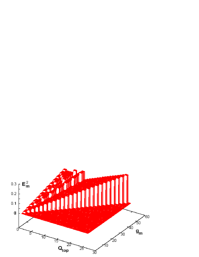
Figure 6: plot of E${}_{m}^{2}$ as a function of the topological charge $\left|{\small Q}_{top}\right|$ and the degree of degeneracy g_m on a 30$\times$30 lattice 4C .

Recall that the analytic prediction for the eigenvalues of the energy spectrum leads to $E_{m}^{2}=\frac{2\sqrt{3}}{3}m\left|\mathcal{B}\right|$ with $m$ a positive integer. Lattice calculations show also that the degeneracy pattern (39) of these eigenvalues is as follows

$$g_{m}=\left\{\begin{array}[c]{ccc}\left|Q\right|&for\text{ }&m=0\\ 2\left|Q\right|&for&m>0\end{array}\right.$$ (251)

By substituting the background field $\mathcal{B}$ by its expression in terms of the topological charge $Q$ and the area of the supercell, we can rewrite the energy spectrum like,

$$E_{m}^{2}=\frac{4\pi\sqrt{3}}{3L_{1}L_{2}}\left|Q\right|m$$ (252)

As shown on the plot, the states with $E_{0}^{2}=0$, that form a triangle on fig 6, corresponds precisely to the zero modes of the Dirac operator with degree of degeneracy $g_{m}$ growing linearly with $Q$ in complete agreement with the index theorem.

Acknowledgement 1

:
The authors thank the Hassan II Academy of Science and Technology where part of this work has been done. E.H.S thanks the Moroccan Center for Scientific Research and Technology; Project ref URAC09, for support.

References

- (1) M. Atiyah, I.M. Singer, Ann. Math. 93 (1971) 139,
- (2) M. F. Atiyah, R. Bott, V. K. Patodi, On the heat equation and the index theorem, Inv. Math. 19 279 (1973),
- (3) I. Barbour, M. Teper, Phys. Lett. 175B (1986) 445, ELSEVIER. DOI: 10.1016/0370-2693(86)90621-0,
- (4) J. Smit, J.C. Vink, Phys. Lett. 194B (1987) 433, DOI: 10.1016/0370-2693(87)91078-1,
- (5) J. Smit, J.C. Vink, Nucl. Phys. B286 (1987) 485, DOI: 10.1016/0550-3213(87)90451-2
- (6) S. Itoh, Y.Iwasaki, T. Yoshie, Phys. Rev. D36 (1987) 527,
- (7) J.C. Vink, Nucl. Phys. B307 (1988) 549,
- (8) T. Kalkreuter, Phys. Rev. D51 (1995) 1305,
- (9) W. Bardeen, A. Duncan, E. Eichten, H.Thacker, Phys.Rev. D59 (1999) 014507, hep-lat/9705002; Phys.Rev. D57 (1998) 1633-164, hep-lat/9705008,
- (10) David H. Adams, Index of a family of lattice Dirac operators and its relation to the non-abelian anomaly on the lattice, Phys.Rev.Lett.86:200-203,2001, arXiv:hep-lat/9910036,
- (11) F. Karsch, E. Seiler, I.O. Stamatescu, Phys.Lett. B157 (1985) 60 , DOI: 10.1016/0370 -2693(85)91212-2,
- (12) Keun-Young Kim, Bum-Hoon Lee, Hyun Seok Yang, Zero Modes and the Atiyah-Singer Index in Noncommutative Instantons, Phys.Rev. D66 (2002) 025034, arXiv:hep-th/0205010,
- (13) Ting-Wai Chiu, The Index and Axial Anomaly of a lattice Dirac operator, Nucl.Phys.Proc.Suppl.106:715-717,2002, arXiv:hep-lat/0110083,
- (14) David H. Adams, Families index theory for Overlap lattice Dirac operator. I, Nucl.Phys. B624 (2002) 469-484, arXiv:hep-lat/0109019,
- (15) Ali Mostafazadeh, Supersymmetry and the Atiyah-Singer Index Theorem, J.Math.Phys. 35 (1994) 1095-1124, arXiv:hep-th/9309059, J.Math.Phys. 35 (1994) 1125-1138, arXiv:hep-th/9309061, Supersymmetry, Path Integration, and the Atiyah-Singer Index Theorem, arXiv:hep-th/9405048.
- (16) G. V. Dunne, Aspects of Chern-Simons theory, Les Houches Lectures 1998, arXiv:hep-th/9902115,
- (17) Joshua L. Davis, Per Kraus, Akhil Shah, Gravity Dual of a Quantum Hall Plateau Transition, JHEP 0811:020,2008, arXiv:0809.1876,
- (18) Y. Zhang, et al., Phys. Rev. Lett. 96, 136806 (2006),
- (19) Z. Jiang, Y. Zhang, H. L. Stormer, P. Kim , Phys. Rev. Lett. 99, 106802 (2007),
- (20) Dipankar Chakrabarti, Simon Hands, Antonio Rago, Topological Aspects of Fermions on a Honeycomb Lattice, JHEP 0906:060,2009, arXiv:0904.1310
- (21) Michael Creutz, Four dimensional graphene and chiral fermions, JHEP 0804: 017, 2008, arXiv:0712.1201,
- (22) A.Borici, Phys. Rev. D78 (2008) 074504, [arXiv:0712.4401],
- (23) P.F Bedaque, M.I Buchoff, B.C Tiburzi, A.Walker-Loud, Phys. Rev. D78 (2008) 017502,[arXiv:0804.1145],
- (24) P.F.Bedaque, M.I.Buchoff, B.C.Tiburzi, A.Walker-Loud, Phys. Lett. B662 (2008) 449, [arXiv:0801.3361],
- (25) L.B Drissi, E.H Saidi, M. Bousmina, 4D Graphene, Phys.Rev.D84:014504,2011, arXiv:1106.5222,
- (26) El Hassan Saidi, On Flavor Symmetry in Lattice Quantum Chromodynamics, J. Math. Phys. 53, 022302 (2012), arXiv:1203.6004,
- (27) L.B Drissi, E.H Saidi, Dirac Zero Modes in Hyperdiamond Model, Phys.Rev.D84:014509,2011, arXiv:1103.1316
- (28) L.B Drissi, H. Mhamdi, E.H Saidi, Anomalous Quantum Hall Effect of 4D Graphene in Background Fields, JHEP 026, 1110 (2011), arXiv:1106.5578, DOI: 10.1007,
- (29) L.B Drissi, E.H Saidi, M. Bousmina, Electronic Properties and Hidden Symmetries of Graphene, Nucl.Phys.B829:523-533,2010, arXiv:1008.4470,
- (30) Lalla Btissam Drissi, El Hassan Saidi, Mosto Bousmina, Graphene and Cousin Systems, in Graphene Simulation”Edited by: J.R. Gong, InTech Publishing, Rijeka, Croatia, (2011), arXiv:1108.1748,
- (31) K. S. Novoselov, Z. Jiang, Y. Zhang, S. V. Morozov, H.L. Stormer, U. Zeitler, J. C. Maan, G. S. Boebinger, P.Kim and A. K. Geim 2007 Science 315 1379,
- (32) Yafis Barlas, Kun Yang, A. H. MacDonald, Quantum Hall Effects in Graphene-Based Two-Dimensional Electron Systems, Nanotechnology 23 052001 (2012), arXiv:1110.1069,
- (33) D. R. Hofstadter, Phys. Rev. B 14, 2239-2249 (1976),
- (34) D. J. Thouless, M. Kohmoto, M. P. Nightingale, M. Nijs, Quantized Hall Conductance in a Two-Dimensional Periodic Potential. Phys. Rev. Lett. 49, 405-408 (1982),
- (35) Mahito Kohmoto, Topological invariant and the quantization of the Hall conductance, Ann. Phys. (N.Y.) 160 (1985) 343,
- (36) Giuseppe De Nittis, Giovanni Landi, Topological aspects of generalized Harper operators, To appear in: ”The Eight International Conference on Progress in Theoretical Physics”, Mentouri University, Constantine, Algeria, October 2011; Conference proceedings of the AIP, edited by N. Mebarki and J. Mimouni, arXiv:1202.0902.
- (37) D. H. Adams, Phys. Rev. Lett. 104, 141602 (2010) [arXiv:0912.2850],
- (38) D. H. Adams, Phys. Lett. B 699:394-397,2011, [arXiv:1008.2833],
- (39) Michael Creutz, Taro Kimura, Tatsuhiro Misumi, Index Theorem and Overlap Formalism with Naive and Minimally Doubled Fermions, JHEP 1012:041,2010, arXiv:1011.0761,
- (40) Michael Creutz, Taro Kimura, Tatsuhiro Misumi, Aoki Phases in the Lattice Gross-Neveu Model with Flavored Mass terms, Phys.Rev.D83:094506,2011, arXiv:1101.4239,
- (41) David H. Adams, Index and overlap construction for staggered fermions, Proceedings contribution for 28th International Symposium on Lattice Field Theory, Lattice2010, June 14-19, 2010, Villasimius, Italy, Journal-ref: PoS (Lattice 2010) 073, arXiv:1103.6191,
- (42) Michael Creutz, Confinement, chiral symmetry, and the lattice, Acta Physica Slovaca 61, No.1, 1-127 (2011), arXiv:1103.3304,
- (43) A.H.Castro-Neto et al. Rev. Mod. Phys.81, 109 (2009),
- (44) Michael Creutz, Minimal doubling and point splitting, PoS Lattice 2010: 078, 2010, arXiv:1009.3154,
- (45) L.B Drissi, E.H Saidi, M. Bousmina, J. Math. Phys. 52, 022306 (2011),
- (46) L. Del Debbio, L. Giusti, M. L¨uscher, R. Petronzio and N. Tantalo, Stability of lattice QCD simulations and the thermodynamic limit, JHEP 0602, 011 (2006), arXiv:hep-lat/0512021.