The kinetic helicity needed to drive large-scale dynamos

Abstract

Magnetic field generation on scales large compared with the scale of the turbulent eddies is known to be possible via the so-called $\alpha$ effect when the turbulence is helical and if the domain is large enough for the $\alpha$ effect to dominate over turbulent diffusion. Using three-dimensional turbulence simulations, we show that the energy of the resulting mean magnetic field of the saturated state increases linearly with the product of normalized helicity and the ratio of domain scale to eddy scale, provided this product exceeds a critical value of around unity. This implies that large-scale dynamo action commences when the normalized helicity is larger than the inverse scale ratio. Our results show that the emergence of small-scale dynamo action does not have any noticeable effect on the large-scale dynamo. Recent findings by Pietarila Graham et al. (2012, Phys. Rev. E85, 066406) of a smaller minimal helicity may be an artifact due to the onset of small-scale dynamo action at large magnetic Reynolds numbers. However, the onset of large-scale dynamo action is difficult to establish when the kinetic helicity is small. Instead of random forcing, they used an ABC-flow with time-dependent phases. We show that such dynamos saturate prematurely in a way that is reminiscent of inhomogeneous dynamos with internal magnetic helicity fluxes. Furthermore, even for very low fractional helicities, such dynamos display large-scale fields that change direction, which is uncharacteristic of turbulent dynamos.

I Introduction

The origin of magnetic fields in astrophysical bodies like the Earth, the Sun and galaxies is studied in the field of dynamo theory. The temporal variation and strength of those fields rules out a primordial origin, through which the magnetic field would have been created in the early Universe. For magnetic fields with energies of the equipartition value, i.e. the turbulent kinetic energy of the medium, the primordial hypothesis explains their strength after creation, but falls short of explaining how the field outlives billions of years of resistive decay [1].

In dynamo theory, astrophysical plasmas are considered sufficiently well conducting fluids where the inertia of the charge-carrying particles can be neglected. In this approximation the equations of magnetohydrodynamics (MHD) provide an adequate model of the medium. In this framework it has been studied under which conditions magnetic fields of equipartition strength and scales larger than the turbulent motions are created and sustained [2].

A successful theoretical model describing the dynamo’s behavior is the mean-field theory. It relates the small-scale turbulent motions to the mean magnetic field via the so-called $\alpha$ effect, which provides the energy input via helical turbulent forcing. During the kinematic phase, i.e. negligible back reaction of the magnetic field on the fluid, the $\alpha$ effect gives a positive feedback on the large-scale magnetic field, which results in its exponential growth. Already the consideration of the kinematic MHD equations with negligible Lorentz force sheds light on the growth rate of the different modes of the magnetic field during the kinematic phase. In the kinematic phase the growth rate $\lambda$ at wave number $k$ is given by [2]

$$\lambda=\alpha k-\eta_{\rm T}k^{2}=(C_{\alpha}-1)\eta_{\rm T}k^{2},$$ (1)

where $C_{\alpha}=\alpha/(\eta_{\rm T}k)$ is the relevant dynamo number for the $\alpha^{2}$ dynamo, $\alpha$ is the $\alpha$ coefficient which is proportional to the small-scale kinetic helicity, and $\eta_{\rm T}=\eta+\eta_{\rm t}$ is the sum of molecular and turbulent magnetic diffusivity. Clearly, dynamo action occurs when $|C_{\alpha}|>C_{\alpha}^{\rm crit}$, where the onset condition is $C_{\alpha}^{\rm crit}=1$. Standard estimates for isotropic turbulence in the high conductivity limit [3, 2] yield $\alpha\approx-(\tau/3)\langle\mathchoice{\mbox{\boldmath$\displaystyle\omega$}}{\mbox{\boldmath$\textstyle\omega$}}{\mbox{\boldmath$\scriptstyle\omega$}}{\mbox{\boldmath$\scriptscriptstyle\omega$}}{}\cdot\mathchoice{\mbox{\boldmath$\displaystyle u$}}{\mbox{\boldmath$\textstyle u$}}{\mbox{\boldmath$\scriptstyle u$}}{\mbox{\boldmath$\scriptscriptstyle u$}}{}\rangle$ and $\eta_{\rm t}\approx(\tau/3)\langle\mathchoice{\mbox{\boldmath$\displaystyle u$}}{\mbox{\boldmath$\textstyle u$}}{\mbox{\boldmath$\scriptstyle u$}}{\mbox{\boldmath$\scriptscriptstyle u$}}{}^{2}\rangle$, where $\tau$ is the correlation time of the turbulence, $\mathchoice{\mbox{\boldmath$\displaystyle\omega$}}{\mbox{\boldmath$\textstyle\omega$}}{\mbox{\boldmath$\scriptstyle\omega$}}{\mbox{\boldmath$\scriptscriptstyle\omega$}}{}=\mathchoice{\mbox{\boldmath$\displaystyle\nabla$}}{\mbox{\boldmath$\textstyle\nabla$}}{\mbox{\boldmath$\scriptstyle\nabla$}}{\mbox{\boldmath$\scriptscriptstyle\nabla$}}{}\times\mathchoice{\mbox{\boldmath$\displaystyle u$}}{\mbox{\boldmath$\textstyle u$}}{\mbox{\boldmath$\scriptstyle u$}}{\mbox{\boldmath$\scriptscriptstyle u$}}{}$ is the vorticity and $\textstyle u$ is the velocity in the small-scale fields. Here, $\langle.\rangle$ denotes a volume average. Using $\eta_{\rm t}\gg\eta$, we have

$$C_{\alpha}\approx-\langle\mathchoice{\mbox{\boldmath$\displaystyle\omega$}}{\mbox{\boldmath$\textstyle\omega$}}{\mbox{\boldmath$\scriptstyle\omega$}}{\mbox{\boldmath$\scriptscriptstyle\omega$}}{}\cdot\mathchoice{\mbox{\boldmath$\displaystyle u$}}{\mbox{\boldmath$\textstyle u$}}{\mbox{\boldmath$\scriptstyle u$}}{\mbox{\boldmath$\scriptscriptstyle u$}}{}\rangle/(k\langle\mathchoice{\mbox{\boldmath$\displaystyle u$}}{\mbox{\boldmath$\textstyle u$}}{\mbox{\boldmath$\scriptstyle u$}}{\mbox{\boldmath$\scriptscriptstyle u$}}{}^{2}\rangle).$$ (2)

It is convenient to define $\langle\mathchoice{\mbox{\boldmath$\displaystyle\omega$}}{\mbox{\boldmath$\textstyle\omega$}}{\mbox{\boldmath$\scriptstyle\omega$}}{\mbox{\boldmath$\scriptscriptstyle\omega$}}{}\cdot\mathchoice{\mbox{\boldmath$\displaystyle u$}}{\mbox{\boldmath$\textstyle u$}}{\mbox{\boldmath$\scriptstyle u$}}{\mbox{\boldmath$\scriptscriptstyle u$}}{}\rangle/(k_{\rm f}\langle\mathchoice{\mbox{\boldmath$\displaystyle u$}}{\mbox{\boldmath$\textstyle u$}}{\mbox{\boldmath$\scriptstyle u$}}{\mbox{\boldmath$\scriptscriptstyle u$}}{}^{2}\rangle)$ as the normalized kinetic helicity, $\epsilon_{\rm f}$, so $C_{\alpha}\approx-\epsilon_{\rm f}k_{\rm f}/k$. This scaling implies that the critical value of the normalized helicity $\epsilon_{\rm f}$ scales inversely proportional to the scale separation ratio, i.e. $\epsilon_{\rm f}^{\rm crit}\propto(k_{\rm f}/k)^{-1}$, where $k\ll k_{\rm f}$ is the wave number of the resulting large-scale magnetic field. This wave number can be equal to $k=k_{1}\equiv 2\pi/L$, which is the smallest wave number in a periodic domain of size $L$.

In summary, the critical dynamo number $C_{\alpha}^{\rm crit}$, which decides between growing or decaying solutions of the large-scale dynamo (LSD), is proportional to the product of normalized helicity $\epsilon_{\rm f}$ and scale separation ratio $k_{\rm f}/k$. Therefore, the amount of helicity needed for the LSD is inversely proportional to the scale separation ratio, and not some higher power of it. It should be noted that the normalized kinetic helicity $\epsilon_{\rm f}$ used here is not the same as the relative kinetic helicity, $\tilde{\epsilon}_{\rm f}=\langle\mathchoice{\mbox{\boldmath$\displaystyle\omega$}}{\mbox{\boldmath$\textstyle\omega$}}{\mbox{\boldmath$\scriptstyle\omega$}}{\mbox{\boldmath$\scriptscriptstyle\omega$}}{}\cdot\mathchoice{\mbox{\boldmath$\displaystyle u$}}{\mbox{\boldmath$\textstyle u$}}{\mbox{\boldmath$\scriptstyle u$}}{\mbox{\boldmath$\scriptscriptstyle u$}}{}\rangle/(\omega_{\rm rms}u_{\rm rms})$. The two are related to each other via the relation

$$\tilde{\epsilon}_{\rm f}/\epsilon_{\rm f}=(\mbox{$k_{\omega}$}/k_{\rm f})^{-1},$$ (3)

where $\mbox{$k_{\omega}$}\approx\omega_{\rm rms}/u_{\rm rms}$ is inversely proportional to the Taylor microscale. Here, the subscripts rms refer to root-mean-square values. For small Reynolds numbers, $k_{\omega}$ provides a useful estimate of the wave number $k_{\rm f}$ of the energy-carrying eddies. In contrast, for large Reynolds numbers Re, we expect $\mbox{$k_{\omega}$}/k_{\rm f}$ to be proportional to $\mbox{\rm Re}^{1/2}$, so $\tilde{\epsilon}_{\rm f}$ decreases correspondingly while $\epsilon_{\rm f}$ remains unchanged.

To understand the saturation of a helical dynamo, it is important to understand the relation between the resulting large-scale field and the associated small-scale field. Indeed, the growth of the large-scale field is always accompanied by a growth of small-scale magnetic field. Small-scale here means the scale of the underlying turbulent motions, which drive the dynamo. Conservation of total magnetic helicity causes a build-up of magnetic helicity at large scales and of opposite sign at small scales [4, 5]. As the dynamo saturates, the largest scales of the magnetic field become even larger, which finally leads to a field of a scale that is similar to that of the system itself. This can be understood as being the result of an inverse cascade, which was first predicted based on closure calculations [6].

If the domain is closed or periodic, the build-up of small-scale magnetic helicity causes the $\alpha$ effect to diminish, which marks the end of the exponential growth and could occur well before final saturation is reached. The dynamo then is said to be catastrophically quenched and, in a closed or periodic system, the subsequent growth to the final state happens not on a dynamical timescale, but on a resistive one. Quenching becomes stronger as the magnetic Reynolds number increases, which, for astrophysically relevant problems, means a total loss of the LSD within the timescales of interest. In the case of open boundaries magnetic helicity fluxes can occur, which can alleviate the quenching and allow for fast saturation of the large-scale magnetic field [7, 8, 9, 10].

In a recent publication [11] it was argued that for periodic boundaries the critical value of $\epsilon_{\rm f}$ for LSD action to occur decreases with the scale separation ratio like $\epsilon_{\rm f}^{\rm crit}\propto(k_{\rm f}/k_{1})^{-3}$. Their finding, however, is at variance with the predictions made using equation (1), which would rather suggest a dependence of $\epsilon_{\rm f}^{\rm crit}\propto(k_{\rm f}/k_{1})^{-1}$ with $C_{\alpha}^{\rm crit}=1$. This discrepancy could be a consequence of the criterion used in [11] for determining $C_{\alpha}^{\rm crit}$. The authors looked at the growth rate of the magnetic field after the end of the kinematic growth phase, but only at a small fraction of the resistive time. Therefore their results might well be contaminated by magnetic fields resulting from the small-scale dynamo (SSD). Earlier simulations [12] have demonstrated that for $\mbox{\rm Re}_{\rm M}\geq 100$, the growth rate of the helical LSD approaches the well-known scaling of the nonhelical SSD with $\lambda\propto\mbox{\rm Re}^{1/2}$, which corresponds to the turnover rate of the smallest turbulent eddies [13, 14].

Given that the LSD is best seen in the nonlinear regime [15], we decided to determine $C_{\alpha}^{\rm crit}$ from a bifurcation diagram by extrapolating to zero. In a bifurcation diagram, we plot the energy of the mean or large-scale field versus $C_{\alpha}$. Simple considerations using the magnetic helicity equation applied to a homogeneous system in the steady state show that the current helicity must vanish [15]. In a helically driven system, this implies that the current helicity of the large-scale field must then be equal to minus the current helicity of the small-scale field. For a helical magnetic field, the normalized mean square magnetic field, $\langle\overline{\bm{B}}^{2}\rangle/B_{\rm eq}^{2}$, is approximately equal to $C_{\alpha}-C_{\alpha}^{\rm crit}$. Here, $B_{\rm eq}=(\mu_{0}\overline{\rho})^{1/2}u_{\rm rms}$ is the equipartition value of the magnetic field, $\mu_{0}$ is the vacuum permeability, and $\overline{\rho}$ is the mean density. Again, since $C_{\alpha}^{\rm crit}\approx 1$ and $C_{\alpha}\approx\epsilon_{\rm f}k_{\rm f}/k_{1}$, this suggests that the LSD is excited for $\epsilon_{\rm f}>(k_{\rm f}/k_{1})^{-1}$ rather than some higher power of $k_{\rm f}/k_{1}$. This is a basic prediction that has been obtained from nonlinear mean-field dynamo models that incorporate magnetic helicity evolution [16] as well as from direct numerical simulations in the presence of shear [17]. It is important to emphasize that mean field dynamo theory has been criticized on the grounds that no $\alpha$ effect may exist in the highly nonlinear regime at large magnetic Reynolds numbers [18]. This is however in conflict with results of numerical simulations using the test-field method [19] showing that $\alpha$ effect and turbulent diffusivity are both large, and that only the difference between both effects is resistively small. Another possibility is that the usual helical dynamo of $\alpha^{2}$ type may not be the fastest growing one [20]. This is related to the fact that, within the framework of the Kazantsev model [21] with helicity, there are new solutions with long-range correlations [22, 23], which could dominate the growth of a large scale field at early times. The purpose of the present paper is therefore to reinvestigate the behavior of solutions in the nonlinear regime over a broader parameter range in the light of recent conflicting findings [11].

II The model

II.1 Basic equations

Following earlier work, we solve the compressible hydromagnetic equations using an isothermal equation of state. Although compressibility is not crucial for the present purpose, it does have the advantage of avoiding the nonlocality associated with solving for the pressure, which requires global communication. Thus, we solve the equations

$$\frac{\partial}{\partial t}\mathchoice{\mbox{\boldmath$\displaystyle A$}}{\mbox{\boldmath$\textstyle A$}}{\mbox{\boldmath$\scriptstyle A$}}{\mbox{\boldmath$\scriptscriptstyle A$}}{}=\mathchoice{\mbox{\boldmath$\displaystyle U$}}{\mbox{\boldmath$\textstyle U$}}{\mbox{\boldmath$\scriptstyle U$}}{\mbox{\boldmath$\scriptscriptstyle U$}}{}\times\mathchoice{\mbox{\boldmath$\displaystyle B$}}{\mbox{\boldmath$\textstyle B$}}{\mbox{\boldmath$\scriptstyle B$}}{\mbox{\boldmath$\scriptscriptstyle B$}}{}-\eta\mu_{0}\mathchoice{\mbox{\boldmath$\displaystyle J$}}{\mbox{\boldmath$\textstyle J$}}{\mbox{\boldmath$\scriptstyle J$}}{\mbox{\boldmath$\scriptscriptstyle J$}}{},$$ (4)

$$\frac{{\rm D}{}}{{\rm D}{}t}\mathchoice{\mbox{\boldmath$\displaystyle U$}}{\mbox{\boldmath$\textstyle U$}}{\mbox{\boldmath$\scriptstyle U$}}{\mbox{\boldmath$\scriptscriptstyle U$}}{}=-c_{\rm s}^{2}\mathchoice{\mbox{\boldmath$\displaystyle\nabla$}}{\mbox{\boldmath$\textstyle\nabla$}}{\mbox{\boldmath$\scriptstyle\nabla$}}{\mbox{\boldmath$\scriptscriptstyle\nabla$}}{}\ln{\rho}+\frac{1}{\rho}\mathchoice{\mbox{\boldmath$\displaystyle J$}}{\mbox{\boldmath$\textstyle J$}}{\mbox{\boldmath$\scriptstyle J$}}{\mbox{\boldmath$\scriptscriptstyle J$}}{}\times\mathchoice{\mbox{\boldmath$\displaystyle B$}}{\mbox{\boldmath$\textstyle B$}}{\mbox{\boldmath$\scriptstyle B$}}{\mbox{\boldmath$\scriptscriptstyle B$}}{}+\mathchoice{\mbox{\boldmath$\displaystyle F$}}{\mbox{\boldmath$\textstyle F$}}{\mbox{\boldmath$\scriptstyle F$}}{\mbox{\boldmath$\scriptscriptstyle F$}}_{\rm visc}+\mathchoice{\mbox{\boldmath$\displaystyle f$}}{\mbox{\boldmath$\textstyle f$}}{\mbox{\boldmath$\scriptstyle f$}}{\mbox{\boldmath$\scriptscriptstyle f$}},$$ (5)

$$\frac{{\rm D}{}}{{\rm D}{}t}\ln{\rho}=-\mathchoice{\mbox{\boldmath$\displaystyle\nabla$}}{\mbox{\boldmath$\textstyle\nabla$}}{\mbox{\boldmath$\scriptstyle\nabla$}}{\mbox{\boldmath$\scriptscriptstyle\nabla$}}{}\cdot\mathchoice{\mbox{\boldmath$\displaystyle U$}}{\mbox{\boldmath$\textstyle U$}}{\mbox{\boldmath$\scriptstyle U$}}{\mbox{\boldmath$\scriptscriptstyle U$}}{},$$ (6)

where $\textstyle A$ is the magnetic vector potential, $\textstyle U$ the velocity, $\textstyle B$ the magnetic field, $\eta$ the molecular magnetic diffusivity, $\mu_{0}$ the vacuum permeability, $\textstyle J$ the electric current density, $c_{\rm s}$ the isothermal sound speed, $\rho$ the density, $\mathchoice{\mbox{\boldmath$\displaystyle F$}}{\mbox{\boldmath$\textstyle F$}}{\mbox{\boldmath$\scriptstyle F$}}{\mbox{\boldmath$\scriptscriptstyle F$}}_{\rm visc}$ the viscous force, $\textstyle f$ the helical forcing term, and ${\rm D}{}/{\rm D}{}t=\partial/\partial t+\mathchoice{\mbox{\boldmath$\displaystyle U$}}{\mbox{\boldmath$\textstyle U$}}{\mbox{\boldmath$\scriptstyle U$}}{\mbox{\boldmath$\scriptscriptstyle U$}}{}\cdot\mathchoice{\mbox{\boldmath$\displaystyle\nabla$}}{\mbox{\boldmath$\textstyle\nabla$}}{\mbox{\boldmath$\scriptstyle\nabla$}}{\mbox{\boldmath$\scriptscriptstyle\nabla$}}{}$ the advective time derivative. The viscous force is given as $\mathchoice{\mbox{\boldmath$\displaystyle F$}}{\mbox{\boldmath$\textstyle F$}}{\mbox{\boldmath$\scriptstyle F$}}{\mbox{\boldmath$\scriptscriptstyle F$}}{}_{\rm visc}=\rho^{-1}\mathchoice{\mbox{\boldmath$\displaystyle\nabla$}}{\mbox{\boldmath$\textstyle\nabla$}}{\mbox{\boldmath$\scriptstyle\nabla$}}{\mbox{\boldmath$\scriptscriptstyle\nabla$}}{}\cdot 2\nu\rho\bm{\mathsf{S}}$, where $\nu$ is the kinematic viscosity, and $\bm{\mathsf{S}}$ is the traceless rate of strain tensor with components ${\sf S}_{ij}=\frac{1}{2}(u_{i,j}+u_{j,i})-\frac{1}{3}\delta_{ij}\mathchoice{\mbox{\boldmath$\displaystyle\nabla$}}{\mbox{\boldmath$\textstyle\nabla$}}{\mbox{\boldmath$\scriptstyle\nabla$}}{\mbox{\boldmath$\scriptscriptstyle\nabla$}}{}\cdot\mathchoice{\mbox{\boldmath$\displaystyle U$}}{\mbox{\boldmath$\textstyle U$}}{\mbox{\boldmath$\scriptstyle U$}}{\mbox{\boldmath$\scriptscriptstyle U$}}{}$. Commas denote partial derivatives.

The energy supply for a helically driven dynamo is provided by the forcing function $\mathchoice{\mbox{\boldmath$\displaystyle f$}}{\mbox{\boldmath$\textstyle f$}}{\mbox{\boldmath$\scriptstyle f$}}{\mbox{\boldmath$\scriptscriptstyle f$}}=\mathchoice{\mbox{\boldmath$\displaystyle f$}}{\mbox{\boldmath$\textstyle f$}}{\mbox{\boldmath$\scriptstyle f$}}{\mbox{\boldmath$\scriptscriptstyle f$}}(\mathchoice{\mbox{\boldmath$\displaystyle x$}}{\mbox{\boldmath$\textstyle x$}}{\mbox{\boldmath$\scriptstyle x$}}{\mbox{\boldmath$\scriptscriptstyle x$}}{},t)$, which is a helical function that is random in time. It is defined as

$$\mathchoice{\mbox{\boldmath$\displaystyle f$}}{\mbox{\boldmath$\textstyle f$}}{\mbox{\boldmath$\scriptstyle f$}}{\mbox{\boldmath$\scriptscriptstyle f$}}{}(\mathchoice{\mbox{\boldmath$\displaystyle x$}}{\mbox{\boldmath$\textstyle x$}}{\mbox{\boldmath$\scriptstyle x$}}{\mbox{\boldmath$\scriptscriptstyle x$}}{},t)={\rm Re}\{N\mathchoice{\mbox{\boldmath$\displaystyle f$}}{\mbox{\boldmath$\textstyle f$}}{\mbox{\boldmath$\scriptstyle f$}}{\mbox{\boldmath$\scriptscriptstyle f$}}{}_{\mathchoice{\mbox{\boldmath$\displaystyle k$}}{\mbox{\boldmath$\textstyle k$}}{\mbox{\boldmath$\scriptstyle k$}}{\mbox{\boldmath$\scriptscriptstyle k$}}{}(t)}\exp[{\rm i}\mathchoice{\mbox{\boldmath$\displaystyle k$}}{\mbox{\boldmath$\textstyle k$}}{\mbox{\boldmath$\scriptstyle k$}}{\mbox{\boldmath$\scriptscriptstyle k$}}{}(t)\cdot\mathchoice{\mbox{\boldmath$\displaystyle x$}}{\mbox{\boldmath$\textstyle x$}}{\mbox{\boldmath$\scriptstyle x$}}{\mbox{\boldmath$\scriptscriptstyle x$}}{}+{\rm i}\phi(t)]\},$$ (7)

where $\textstyle x$ is the position vector. The wave vector $\mathchoice{\mbox{\boldmath$\displaystyle k$}}{\mbox{\boldmath$\textstyle k$}}{\mbox{\boldmath$\scriptstyle k$}}{\mbox{\boldmath$\scriptscriptstyle k$}}{}(t)$ and the random phase $-\pi<\phi(t)\leq\pi$ change at every time step, so $\mathchoice{\mbox{\boldmath$\displaystyle f$}}{\mbox{\boldmath$\textstyle f$}}{\mbox{\boldmath$\scriptstyle f$}}{\mbox{\boldmath$\scriptscriptstyle f$}}{}(\mathchoice{\mbox{\boldmath$\displaystyle x$}}{\mbox{\boldmath$\textstyle x$}}{\mbox{\boldmath$\scriptstyle x$}}{\mbox{\boldmath$\scriptscriptstyle x$}}{},t)$ is $\delta$-correlated in time. For the time-integrated forcing function to be independent of the length of the time step $\delta t$, the normalization factor $N$ has to be proportional to $\delta t^{-1/2}$. On dimensional grounds it is chosen to be $N=f_{0}c_{\rm s}(|\mathchoice{\mbox{\boldmath$\displaystyle k$}}{\mbox{\boldmath$\textstyle k$}}{\mbox{\boldmath$\scriptstyle k$}}{\mbox{\boldmath$\scriptscriptstyle k$}}{}|c_{\rm s}/\delta t)^{1/2}$, where $f_{0}$ is a nondimensional forcing amplitude. We choose $f_{0}=0.02$, which results in a maximum Mach number of about 0.3 and an rms value of about 0.085. At each timestep we select randomly one of many possible wave vectors in a certain range around a given forcing wave number. The average wave number is referred to as $k_{\rm f}$. Transverse helical waves are produced via [14]

$$\mathchoice{\mbox{\boldmath$\displaystyle f$}}{\mbox{\boldmath$\textstyle f$}}{\mbox{\boldmath$\scriptstyle f$}}{\mbox{\boldmath$\scriptscriptstyle f$}}{}_{\mathchoice{\mbox{\boldmath$\displaystyle k$}}{\mbox{\boldmath$\textstyle k$}}{\mbox{\boldmath$\scriptstyle k$}}{\mbox{\boldmath$\scriptscriptstyle k$}}{}}=\bm{\mathsf{R}}\cdot\mathchoice{\mbox{\boldmath$\displaystyle f$}}{\mbox{\boldmath$\textstyle f$}}{\mbox{\boldmath$\scriptstyle f$}}{\mbox{\boldmath$\scriptscriptstyle f$}}{}_{\mathchoice{\mbox{\boldmath$\displaystyle k$}}{\mbox{\boldmath$\textstyle k$}}{\mbox{\boldmath$\scriptstyle k$}}{\mbox{\boldmath$\scriptscriptstyle k$}}{}}^{\rm(nohel)}\quad\mbox{with}\quad{\sf R}_{ij}={\delta_{ij}-{\rm i}\sigma\epsilon_{ijk}\hat{k}_{k}\over\sqrt{1+\sigma^{2}}},$$ (8)

where $\sigma$ is a measure of the helicity of the forcing and $\sigma=1$ for positive maximum helicity of the forcing function. Furthermore,

$$\mathchoice{\mbox{\boldmath$\displaystyle f$}}{\mbox{\boldmath$\textstyle f$}}{\mbox{\boldmath$\scriptstyle f$}}{\mbox{\boldmath$\scriptscriptstyle f$}}{}_{\mathchoice{\mbox{\boldmath$\displaystyle k$}}{\mbox{\boldmath$\textstyle k$}}{\mbox{\boldmath$\scriptstyle k$}}{\mbox{\boldmath$\scriptscriptstyle k$}}{}}^{\rm(nohel)}=\left(\mathchoice{\mbox{\boldmath$\displaystyle k$}}{\mbox{\boldmath$\textstyle k$}}{\mbox{\boldmath$\scriptstyle k$}}{\mbox{\boldmath$\scriptscriptstyle k$}}{}\times\mathchoice{\mbox{\boldmath$\displaystyle e$}}{\mbox{\boldmath$\textstyle e$}}{\mbox{\boldmath$\scriptstyle e$}}{\mbox{\boldmath$\scriptscriptstyle e$}}{}\right)/\sqrt{\mathchoice{\mbox{\boldmath$\displaystyle k$}}{\mbox{\boldmath$\textstyle k$}}{\mbox{\boldmath$\scriptstyle k$}}{\mbox{\boldmath$\scriptscriptstyle k$}}{}^{2}-(\mathchoice{\mbox{\boldmath$\displaystyle k$}}{\mbox{\boldmath$\textstyle k$}}{\mbox{\boldmath$\scriptstyle k$}}{\mbox{\boldmath$\scriptscriptstyle k$}}{}\cdot\mathchoice{\mbox{\boldmath$\displaystyle e$}}{\mbox{\boldmath$\textstyle e$}}{\mbox{\boldmath$\scriptstyle e$}}{\mbox{\boldmath$\scriptscriptstyle e$}}{})^{2}}$$ (9)

is a nonhelical forcing function, where $\textstyle e$ is an arbitrary unit vector not aligned with $\textstyle k$; note that $|\mathchoice{\mbox{\boldmath$\displaystyle f$}}{\mbox{\boldmath$\textstyle f$}}{\mbox{\boldmath$\scriptstyle f$}}{\mbox{\boldmath$\scriptscriptstyle f$}}{}_{\mathchoice{\mbox{\boldmath$\displaystyle k$}}{\mbox{\boldmath$\textstyle k$}}{\mbox{\boldmath$\scriptstyle k$}}{\mbox{\boldmath$\scriptscriptstyle k$}}{}}|^{2}=1$ and

$$\mathchoice{\mbox{\boldmath$\displaystyle f$}}{\mbox{\boldmath$\textstyle f$}}{\mbox{\boldmath$\scriptstyle f$}}{\mbox{\boldmath$\scriptscriptstyle f$}}{}_{\mathchoice{\mbox{\boldmath$\displaystyle k$}}{\mbox{\boldmath$\textstyle k$}}{\mbox{\boldmath$\scriptstyle k$}}{\mbox{\boldmath$\scriptscriptstyle k$}}{}}\cdot({\rm i}\mathchoice{\mbox{\boldmath$\displaystyle k$}}{\mbox{\boldmath$\textstyle k$}}{\mbox{\boldmath$\scriptstyle k$}}{\mbox{\boldmath$\scriptscriptstyle k$}}{}\times\mathchoice{\mbox{\boldmath$\displaystyle f$}}{\mbox{\boldmath$\textstyle f$}}{\mbox{\boldmath$\scriptstyle f$}}{\mbox{\boldmath$\scriptscriptstyle f$}}{}_{\mathchoice{\mbox{\boldmath$\displaystyle k$}}{\mbox{\boldmath$\textstyle k$}}{\mbox{\boldmath$\scriptstyle k$}}{\mbox{\boldmath$\scriptscriptstyle k$}}{}})^{*}=2\sigma k/(1+\sigma^{2}),$$ (10)

so the relative helicity of the forcing function in real space is $2\sigma/(1+\sigma^{2})$.

For comparison with earlier work, we shall also use in one case an ABC-flow forcing function [24],

$$\mathchoice{\mbox{\boldmath$\displaystyle f$}}{\mbox{\boldmath$\textstyle f$}}{\mbox{\boldmath$\scriptstyle f$}}{\mbox{\boldmath$\scriptscriptstyle f$}}{}(\mathchoice{\mbox{\boldmath$\displaystyle x$}}{\mbox{\boldmath$\textstyle x$}}{\mbox{\boldmath$\scriptstyle x$}}{\mbox{\boldmath$\scriptscriptstyle x$}}{})={f_{0}\over\sqrt{{3\over 2}(1+\sigma^{2})}}\left(\begin{matrix}\sin X_{3}+\sigma\cos X_{2}\\ \sin X_{1}+\sigma\cos X_{3}\\ \sin X_{2}+\sigma\cos X_{1}\end{matrix}\right),$$ (11)

where $X_{i}=k_{\rm f}x_{i}+\theta_{i}$ and $\theta_{i}=\theta_{0}\cos\omega_{i}t$ are time-dependent phases that vary sinusoidally with frequencies $\omega_{i}$ and amplitude $\theta_{0}$. This forcing function is easy to implement and serves therefore as a proxy of helical turbulence; see Refs. [25, 11], where the phases changed randomly. We have restricted ourselves to the special case where the coefficients in front of the trigonometric functions are unity, but those could be made time-dependent too; see Ref. [26]. However, as we will see below, ABC-flow driven dynamos do not show some crucial aspects of random plane wave-forced helical turbulence. Most of the results presented below concern the forcing function Eq. (7), and only one case with Eq. (11) will be considered at the end.

Our model is governed by several nondimensional parameters. In addition to the scale separation ratio $k_{\rm f}/k_{1}$, introduced above, there are the magnetic Reynolds and Prandtl numbers

$$\mbox{\rm Re}_{\rm M}=u_{\rm rms}/(\eta k_{\rm f}),\quad\mbox{\rm Pr}_{\rm M}=\nu/\eta.$$ (12)

These two numbers also define the fluid Reynolds number, $\mbox{\rm Re}=u_{\rm rms}/(\nu k_{\rm f})=\mbox{\rm Re}_{\rm M}/\mbox{\rm Pr}_{\rm M}$. The maximum values that can be attained are limited by the numerical resolution and become more restrictive at larger scale separation. The calculations have been performed using the Pencil Code (see http://pencil-code.googlecode.com) at resolutions of up to $512^{3}$ mesh points.

II.2 Mean-field interpretation

The induced small-scale motions $\textstyle u$ are helical and give rise to the usual (kinetic) $\alpha$ effect [3]

$$\alpha_{\rm K}\approx-\frac{\langle\mathchoice{\mbox{\boldmath$\displaystyle\omega$}}{\mbox{\boldmath$\textstyle\omega$}}{\mbox{\boldmath$\scriptstyle\omega$}}{\mbox{\boldmath$\scriptscriptstyle\omega$}}{}\cdot\mathchoice{\mbox{\boldmath$\displaystyle u$}}{\mbox{\boldmath$\textstyle u$}}{\mbox{\boldmath$\scriptstyle u$}}{\mbox{\boldmath$\scriptscriptstyle u$}}{}\rangle}{3u_{\rm rms}k_{\rm f}}.$$ (13)

In the nonlinear regime, following the early work of Pouquet, Frisch, and Léorat [27], the relevant $\alpha$ effect for dynamo action is believed to be the sum of the kinetic and a magnetic $\alpha$, i.e.,

$$\alpha\approx\frac{-\langle\mathchoice{\mbox{\boldmath$\displaystyle\omega$}}{\mbox{\boldmath$\textstyle\omega$}}{\mbox{\boldmath$\scriptstyle\omega$}}{\mbox{\boldmath$\scriptscriptstyle\omega$}}{}\cdot\mathchoice{\mbox{\boldmath$\displaystyle u$}}{\mbox{\boldmath$\textstyle u$}}{\mbox{\boldmath$\scriptstyle u$}}{\mbox{\boldmath$\scriptscriptstyle u$}}{}\rangle+\langle\mathchoice{\mbox{\boldmath$\displaystyle j$}}{\mbox{\boldmath$\textstyle j$}}{\mbox{\boldmath$\scriptstyle j$}}{\mbox{\boldmath$\scriptscriptstyle j$}}{}\cdot\mathchoice{\mbox{\boldmath$\displaystyle b$}}{\mbox{\boldmath$\textstyle b$}}{\mbox{\boldmath$\scriptstyle b$}}{\mbox{\boldmath$\scriptscriptstyle b$}}{}\rangle/\langle\rho\rangle}{3u_{\rm rms}k_{\rm f}}.$$ (14)

Simulations have confirmed the basic form of Eq. (14) with equal contributions from $\langle\mathchoice{\mbox{\boldmath$\displaystyle\omega$}}{\mbox{\boldmath$\textstyle\omega$}}{\mbox{\boldmath$\scriptstyle\omega$}}{\mbox{\boldmath$\scriptscriptstyle\omega$}}{}\cdot\mathchoice{\mbox{\boldmath$\displaystyle u$}}{\mbox{\boldmath$\textstyle u$}}{\mbox{\boldmath$\scriptstyle u$}}{\mbox{\boldmath$\scriptscriptstyle u$}}{}\rangle$ and $\langle\mathchoice{\mbox{\boldmath$\displaystyle j$}}{\mbox{\boldmath$\textstyle j$}}{\mbox{\boldmath$\scriptstyle j$}}{\mbox{\boldmath$\scriptscriptstyle j$}}{}\cdot\mathchoice{\mbox{\boldmath$\displaystyle b$}}{\mbox{\boldmath$\textstyle b$}}{\mbox{\boldmath$\scriptstyle b$}}{\mbox{\boldmath$\scriptscriptstyle b$}}{}\rangle/\langle\rho\rangle$, but one may argue that the second term should only exist in the presence of hydromagnetic background turbulence [28], and not if the magnetic fluctuations are a consequence of tangling of a mean field produced by dynamo action as in the simulations in Ref. [15]. However, to explain the resistively slow saturation in those simulations, the only successful explanation [29, 16] comes from considering the magnetic helicity equation, which feeds back onto the $\alpha$ effect via Eq. (14). This is our main argument in support of the applicability of this equation. Another problem with Eq. (14) is the assumption of isotropy [28], which has however been relaxed in subsequent work [30]. Let us also mention that Eq. (14) is usually obtained using the $\tau$ approximation. In its simplest form, it yields incorrect results in the low conductivity limit, where the second-order correlation approximation applies [3, 2]. However, this is just a consequence of making simplifying assumptions in handling the diffusion operator, which can be avoided, too [31]. At higher conductivity, numerical simulations have been able to reproduce some important predictions from the $\tau$ approximation [32].

Equation (14) is used to derive the expression for the resistively slow saturation behavior [29]. We will not reproduce here the derivation, which can be found elsewhere [16]. The resulting large-scale fields can be partially helical, which means one can write

$$\langle\mathchoice{\mbox{\boldmath$\displaystyle J$}}{\mbox{\boldmath$\textstyle J$}}{\mbox{\boldmath$\scriptstyle J$}}{\mbox{\boldmath$\scriptscriptstyle J$}}{}\cdot\mathchoice{\mbox{\boldmath$\displaystyle B$}}{\mbox{\boldmath$\textstyle B$}}{\mbox{\boldmath$\scriptstyle B$}}{\mbox{\boldmath$\scriptscriptstyle B$}}{}\rangle=\epsilon_{\rm m}k_{\rm m}\langle\mathchoice{\mbox{\boldmath$\displaystyle B$}}{\mbox{\boldmath$\textstyle B$}}{\mbox{\boldmath$\scriptstyle B$}}{\mbox{\boldmath$\scriptscriptstyle B$}}{}^{2}\rangle,$$ (15)

with large-scale wave vector $k_{\rm m}$ and corresponding fractional helicity $\epsilon_{\rm m}$, defined through Eq. (15). However, in the cases considered below the domain is triply periodic, so the solutions are Beltrami fields for which $k_{\rm m}\approx k_{1}$ and $\epsilon_{\rm m}\approx 1$ is an excellent approximation, and only $\epsilon_{\rm f}$ will take values less unity. Nevertheless, in some expressions we retain the $\epsilon_{\rm m}$ factor for clarity. For example, the saturation value of the large-scale magnetic field, $B_{\rm sat}$, is given by [16]

$$B_{\rm sat}^{2}/B_{\rm eq}^{2}\approx\left(|C_{\alpha}|/\epsilon_{\rm m}-1\right)\iota,$$ (16)

where $C_{\alpha}=\alpha_{\rm K}/(\eta_{\rm T}k_{1})$ is the relevant dynamo number based on the smallest wavenumber in the domain and $\iota=1+3/\mbox{\rm Re}_{\rm M}\equiv\eta_{\rm T}/\eta_{\rm t}$ is a correction factor resulting from the fact that $\eta_{\rm T}$ is slightly bigger than $\eta_{\rm t}$. The factor $3$ in the expression for $\iota$ results from our definition of $\mbox{\rm Re}_{\rm M}$ and the fact that [33]

$$\eta_{\rm t}\approx u_{\rm rms}/(3k_{\rm f})=\eta\mbox{\rm Re}_{\rm M}/3.$$ (17)

Equation (16) shows clearly the onset condition $|C_{\alpha}|>|\epsilon_{\rm m}|\approx 1$. Using Eqs. (13) and (17), we find

$$C_{\alpha}\approx-{\langle\mathchoice{\mbox{\boldmath$\displaystyle\omega$}}{\mbox{\boldmath$\textstyle\omega$}}{\mbox{\boldmath$\scriptstyle\omega$}}{\mbox{\boldmath$\scriptscriptstyle\omega$}}{}\cdot\mathchoice{\mbox{\boldmath$\displaystyle u$}}{\mbox{\boldmath$\textstyle u$}}{\mbox{\boldmath$\scriptstyle u$}}{\mbox{\boldmath$\scriptscriptstyle u$}}{}\rangle\over\iota k_{1}u_{\rm rms}^{2}}=-{\epsilon_{\rm f}k_{\rm f}\over\iota k_{1}}.$$ (18)

From Eq. (16) we can derive the critical value of the normalized helicity $\epsilon_{\rm f}$ as a function of the scale separation ratio. Setting $C_{\alpha}$ to its critical value ($|C_{\alpha}|=\epsilon_{\rm m}$) we obtain

$$\epsilon_{\rm f}^{\rm crit}\approx\iota\epsilon_{\rm m}\left(\frac{k_{\rm f}}{k_{1}}\right)^{-1},$$ (19)

which is at variance with the findings in Ref. [11].

Once the dynamo is excited and has reached a steady state, not only $\alpha$ but also $\eta_{\rm t}$ will be suppressed. This can be taken into account using a quenching factor $g(\overline{B})$, so $\eta_{\rm t}(\overline{B})=\eta_{\rm t0}g(\overline{B})$ with $g=(1+\tilde{g}|\overline{\bm{B}}|/B_{\rm eq})^{-1}$ [34, 35, 15]. Equation (16) is then modified and reads $B_{\rm sat}^{2}/B_{\rm eq}^{2}=(|C_{\alpha}|-C_{\alpha 0})\iota/\epsilon_{\rm m}$ with

$$C_{\alpha 0}=[1-(1-g)/\iota]\epsilon_{\rm m}.$$ (20)

Note that $C_{\alpha 0}=\epsilon_{\rm m}^{-1}$ in the unquenched case, i.e., for $g=1$.

II.3 Simulation strategy

We recall that our forcing term $\textstyle f$ in equation Eq. (7) is a stochastic forcing centered around the wave number $k_{\rm f}$. In contrast to Ref. [11], this forcing is $\delta$-correlated in time. The fractional helicity of the helical forcing is a free parameter. The simulation domain is a periodic cube with dimensions $2\pi$. Due to the cubic geometry of the domain, the large-scale magnetic field can orient itself in three possible directions. Therefore, we compute three possible planar averages ($xy$, $xz$, and $yz$ averages). From their resistive evolution we infer their saturation values at the end of the resistive phase. The strongest field gives then the relevant mean-field $\overline{\bm{B}}$.

Since $\overline{\bm{B}}$ is helical and magnetic helicity can only change on resistive timescales, the temporal evolution of the energy of the mean magnetic field, $M(t)$, is given by [15]

$$M(t)=M_{0}-M_{1}e^{-t/\tau},$$ (21)

where $\tau^{-1}=2\eta\epsilon_{\rm m}^{2}k_{1}^{2}$ is known, $M_{0}=B_{\rm sat}^{2}$ is the square of the desired saturation field strength, and $M_{1}$ is an unknown constant that can be positive or negative, depending on whether the initial magnetic field of a given calculation was smaller or larger than the final value. (Here, an initial field could refer to the last snapshot of another calculation with similar parameters, for example.) The functional behavior given by Eq. (21) allows us to determine $B_{\rm sat}^{2}$ as the time average of $M+\tau{\rm d}{}M/{\rm d}{}t$, which should only fluctuate about a constant value, i.e.,

$$B_{\rm sat}^{2}\approx{1\over t_{2}-t_{1}}\int_{t_{1}}^{t_{2}}\left[\langle\overline{\bm{B}}^{2}\rangle(t^{\prime})+\tau{{\rm d}{}\over{\rm d}{}t^{\prime}}\langle\overline{\bm{B}}^{2}\rangle\right]\,{\rm d}{}t^{\prime}.$$ (22)

This technique has the advantage that we do not need to wait until the field reaches its final saturation field strength. Error bars can be estimated by computing this average for each third of the full time series and taking the largest departure from the average over the full time series. An example is shown in Fig. 1, where we see $\langle\overline{\bm{B}}^{2}\rangle$ still growing while $\langle\overline{\bm{B}}^{2}\rangle+\tau{\rm d}{}\langle\overline{\bm{B}}^{2}\rangle/{\rm d}{}t$ is nearly constant when $\langle\overline{\bm{B}}^{2}\rangle$ reaches a value less than half its final one. This figure shows that the growth of $\langle\overline{\bm{B}}^{2}\rangle$ follows the theoretical expectation Eq. (21) quite closely and that temporal fluctuations about this value are small, as can be seen by the fact that its time derivative fluctuates only little.

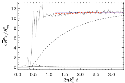
Figure 1: (Color online) Example showing the evolution of the normalized $\langle\overline{\bm{B}}^{2}\rangle$ (dashed) and that of $\langle\overline{\bm{B}}^{2}\rangle+\tau{\rm d}{}\langle\overline{\bm{B}}^{2}\rangle/{\rm d}{}t$ (dotted), compared with its average in the interval $1.2\leq 2\eta k_{1}^{2}t\leq 3.5$ (horizontal blue solid line), as well as averages over three subintervals (horizontal red dashed lines). Here, $\overline{\bm{B}}$ is evaluated as an $xz$ average, $\langle\mathchoice{\mbox{\boldmath$\displaystyle B$}}{\mbox{\boldmath$\textstyle B$}}{\mbox{\boldmath$\scriptstyle B$}}{\mbox{\boldmath$\scriptscriptstyle B$}}{}\rangle_{xz}$. For comparison we also show the other two averages, $\langle\mathchoice{\mbox{\boldmath$\displaystyle B$}}{\mbox{\boldmath$\textstyle B$}}{\mbox{\boldmath$\scriptstyle B$}}{\mbox{\boldmath$\scriptscriptstyle B$}}{}\rangle_{xy}$ (solid) and $\langle\mathchoice{\mbox{\boldmath$\displaystyle B$}}{\mbox{\boldmath$\textstyle B$}}{\mbox{\boldmath$\scriptstyle B$}}{\mbox{\boldmath$\scriptscriptstyle B$}}{}\rangle_{yz}$ (dash-dotted), but their values are very small.

III Results

III.1 Dependence of kinetic helicity on $\sigma$

We recall that the relative helicity of the forcing function is $\langle\mathchoice{\mbox{\boldmath$\displaystyle f$}}{\mbox{\boldmath$\textstyle f$}}{\mbox{\boldmath$\scriptstyle f$}}{\mbox{\boldmath$\scriptscriptstyle f$}}{}\cdot\mathchoice{\mbox{\boldmath$\displaystyle\nabla$}}{\mbox{\boldmath$\textstyle\nabla$}}{\mbox{\boldmath$\scriptstyle\nabla$}}{\mbox{\boldmath$\scriptscriptstyle\nabla$}}{}\times\mathchoice{\mbox{\boldmath$\displaystyle f$}}{\mbox{\boldmath$\textstyle f$}}{\mbox{\boldmath$\scriptstyle f$}}{\mbox{\boldmath$\scriptscriptstyle f$}}{}\rangle/[\mathchoice{\mbox{\boldmath$\displaystyle f$}}{\mbox{\boldmath$\textstyle f$}}{\mbox{\boldmath$\scriptstyle f$}}{\mbox{\boldmath$\scriptscriptstyle f$}}{}_{\rm rms}(\mathchoice{\mbox{\boldmath$\displaystyle\nabla$}}{\mbox{\boldmath$\textstyle\nabla$}}{\mbox{\boldmath$\scriptstyle\nabla$}}{\mbox{\boldmath$\scriptscriptstyle\nabla$}}{}\times\mathchoice{\mbox{\boldmath$\displaystyle f$}}{\mbox{\boldmath$\textstyle f$}}{\mbox{\boldmath$\scriptstyle f$}}{\mbox{\boldmath$\scriptscriptstyle f$}}{})_{\rm rms}]=2\sigma/(1+\sigma^{2})$. This imposes then a similar variation onto the relative kinetic helicity, $\tilde{\epsilon}_{\rm f}=\langle\mathchoice{\mbox{\boldmath$\displaystyle\omega$}}{\mbox{\boldmath$\textstyle\omega$}}{\mbox{\boldmath$\scriptstyle\omega$}}{\mbox{\boldmath$\scriptscriptstyle\omega$}}{}\cdot\mathchoice{\mbox{\boldmath$\displaystyle u$}}{\mbox{\boldmath$\textstyle u$}}{\mbox{\boldmath$\scriptstyle u$}}{\mbox{\boldmath$\scriptscriptstyle u$}}{}\rangle/(\omega_{\rm rms}u_{\rm rms})$; see Fig. 2(a). However, as discussed above, $\tilde{\epsilon}_{\rm f}$ is smaller than $\epsilon_{\rm f}$ by a factor $\mbox{$k_{\omega}$}/k_{\rm f}$, which in turn depends on the Reynolds number (see below). It turns out that $\epsilon_{\rm f}$ matches almost exactly the values of $2\sigma/(1+\sigma^{2})$; see Fig. 2(b).

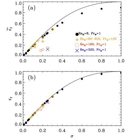
Figure 2: (Color online) Dependence of relative kinetic helicity $\tilde{\epsilon}_{\rm f}$ (a) and normalized kinetic helicity $\epsilon_{\rm f}$ (b) on the helicity parameter $\sigma$ of the forcing function Eq. (8) together with the analytical expression $2\sigma/(1+\sigma^{2})$ (solid line).

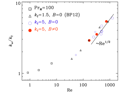
Figure 3: (Color online) Dependence of $\mbox{$k_{\omega}$}/k_{\rm f}$ on Re. The open and closed circles correspond to runs with $\mbox{\rm Pr}_{\rm M}=1$ without and with magnetic field, respectively, while squares correspond to runs with $\mbox{\rm Pr}_{\rm M}=100$ and $\mbox{\rm Re}=\mbox{\rm Re}_{\rm M}/\mbox{\rm Pr}_{\rm M}$ is small. Triangles denote the results for $k_{\rm f}/k_{1}=1.5$ of Ref. [36] (BP12).

The theoretically expected scaling $\mbox{$k_{\omega}$}/k_{\rm f}\propto\mbox{\rm Re}^{1/2}$ is a well-known result for high Reynolds number turbulence [37], and has recently been verified using simulations similar to those presented here, but without magnetic field and a smaller scale separation ratio of $k_{\rm f}/k_{1}=1.5$ [36]. For our current data we find that such a scaling is obeyed for $\mbox{\rm Pr}_{\rm M}=1$ and large values of Re, independently of the presence of magnetic field or kinetic helicity, but this scaling is not obeyed when $\mbox{\rm Pr}_{\rm M}=100$ and Re is small; see Fig. 3.

III.2 Dependence on scale separation

Next, we perform simulations with different forcing wave numbers $k_{\rm f}$ and different values of $\epsilon_{\rm f}$ at approximately constant magnetic Reynolds number, $\mbox{\rm Re}_{\rm M}\approx 6$, and fixed magnetic Prandtl number, $\mbox{\rm Pr}_{\rm M}=1$. Near the end of the resistive saturation phase we look at the energy of the strongest mode at $k=k_{1}$, using the method described in Sec. II.3. We choose this rather small value of Re because we want to access relatively large scale separation ratios of up to $k_{\rm f}/k_{1}=80$. Given that the Reynolds number based on the scale of the domain is limited by the number of mesh points (500, say), it follows that for $k_{\rm f}/k_{1}=80$ the Reynolds number defined through Eq. (12) is 6. For comparison, a Reynolds number based on the size of the domain, i.e., $u_{\rm rms}L/\eta$, would be larger by a factor $2\pi$, i.e., 3000.

As seen from Eq. (16), mean-field considerations predict a linear increase of the saturation magnetic energy with $C_{\alpha}$ and onset at $C_{\alpha}=1$. This behavior is reproduced in our simulation (Fig. 4), where we compare the theoretical prediction with the simulation results. For different values of $k_{\rm f}/k_{1}$ and $C_{\alpha}$ we extrapolate the critical value $C_{\alpha}^{\rm crit}\approx 1.2$ (Fig. 4), which gives the critical values $\epsilon_{\rm f}^{\rm crit}\approx 1.2\iota\,(k_{\rm f}/k_{1})^{-1}=1.7\,(k_{\rm f}/k_{1})^{-1}$ for which the LSD is excited. For each scale separation value we plot the dependence of $\langle\overline{\bm{B}}^{2}\rangle/B_{\rm eq}^{2}$ on $\epsilon_{\rm f}$ (Fig. 5) and make linear fits. From these fits we can extrapolate the critical values $\epsilon_{\rm f}^{\rm crit}$, for which the LSD gets excited (Fig. 6), which gives again $\epsilon_{\rm f}^{\rm crit}\approx 1.7\,(k_{\rm f}/k_{1})^{-1}$.

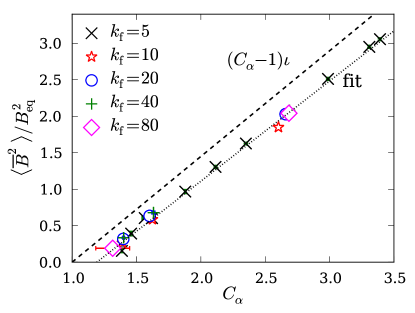
Figure 4: (Color online) Steady state values of $\langle\overline{\bm{B}}^{2}\rangle/B_{\rm eq}^{2}$ as a function of $C_{\alpha}$ together with the theoretical prediction from Eq. (16) (dashed line) and a linear fit (dotted line).

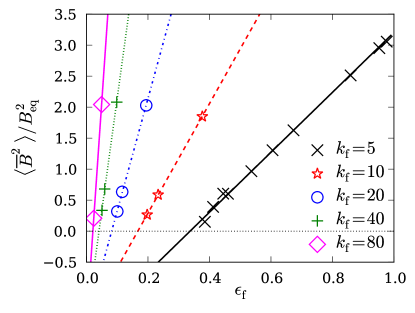
Figure 5: (Color online) Steady state values of $\langle\overline{\bm{B}}^{2}\rangle/B_{\rm eq}^{2}$ as a function of $\epsilon_{\rm f}$ for various scale separation values $k_{\rm f}/k_{1}$ together with linear fits.

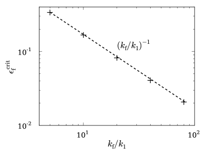
Figure 6: Critical value for the normalized kinetic helicity $\epsilon_{\rm f}$ for which LSD action occurs for different scale separations.

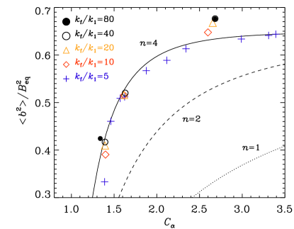
Figure 7: (Color online) Steady state values of $\langle\mathchoice{\mbox{\boldmath$\displaystyle b$}}{\mbox{\boldmath$\textstyle b$}}{\mbox{\boldmath$\scriptstyle b$}}{\mbox{\boldmath$\scriptscriptstyle b$}}{}^{2}\rangle/B_{\rm eq}^{2}$ as a function of $C_{\alpha}$ together with the fit formula from Eq. (23) with $n=4$, compared with $n=1$ (dotted) and $n=2$ (dashed). Different symbols denote different values of $k_{\rm f}/k_{1}$.

It is noteworthy that the graph of $\langle\overline{\bm{B}}^{2}\rangle/B_{\rm eq}^{2}$ versus $C_{\alpha}$ deviates systematically (although only by a small amount) from the theoretically expected value, $(C_{\alpha}-1)\iota$. While the slope is rather close to the expected one, the LSD onset is slightly delayed and occurs at $C_{\alpha}\approx 1.2$ instead of 1. The reason for this is not clear, although one might speculate that it could be modeled by adopting modified effective values of $\iota$ or $\epsilon_{\rm m}$ in Eq. (20). Apart from such minor discrepancies with respect to the simple theory, the agreement is quite remarkable. Nevertheless, we must ask ourselves whether this agreement persists for larger values of the magnetic Reynolds number. This will be addressed in Sec. III.3.

At this point we should note that there is also a theoretical prediction for the energy in the magnetic fluctuations, namely $\langle\mathchoice{\mbox{\boldmath$\displaystyle b$}}{\mbox{\boldmath$\textstyle b$}}{\mbox{\boldmath$\scriptstyle b$}}{\mbox{\boldmath$\scriptscriptstyle b$}}{}^{2}\rangle/B_{\rm eq}^{2}\approx(C_{\alpha}-C_{\alpha}^{\rm crit})/C_{\alpha}$. Nonetheless, the results shown in Fig. 7 deviate from this relation and are better described by a modified formula

$$\langle\mathchoice{\mbox{\boldmath$\displaystyle b$}}{\mbox{\boldmath$\textstyle b$}}{\mbox{\boldmath$\scriptstyle b$}}{\mbox{\boldmath$\scriptscriptstyle b$}}{}^{2}\rangle/B_{\rm eq}^{2}\propto 1-({C_{\alpha}^{\rm crit}/C_{\alpha}})^{n}\quad\mbox{(with $n\approx 4$)}.$$ (23)

Again, the reason for this departure is currently unclear.

III.3 Dependence on $\mbox{\rm Re}_{\rm M}$

To examine whether there is any unexpected dependence of the onset and the energy of the mean magnetic field on $\mbox{\rm Re}_{\rm M}$ and to approach the parameters used in Ref. [11], who used values up to $\mbox{\rm Re}_{\rm M}=1500$, we now consider larger values of the magnetic Reynolds number. This widens the inertial range significantly and leads to the excitation of the SSD. We consider first the case of a large magnetic Prandtl number ($\mbox{\rm Pr}_{\rm M}=100$) and turn then to the more usual case of $\mbox{\rm Pr}_{\rm M}=1$. Our motivation behind the first case is that higher values of $\mbox{\rm Re}_{\rm M}$ can more easily be reached at larger values of $\mbox{\rm Pr}_{\rm M}$. This is because at large values of $\mbox{\rm Pr}_{\rm M}$, most of the injected energy is dissipated viscously rather than resistively, leaving less energy to be channeled down the magnetic cascade [38]. This is similar to the case of small values of $\mbox{\rm Pr}_{\rm M}$, where larger fluid Reynolds numbers can be reached because then most of the energy is dissipated resistively [12]. Here, however, we shall first be concerned with the former case of large values of $\mbox{\rm Pr}_{\rm M}$ and consider then the case of $\mbox{\rm Pr}_{\rm M}=1$.

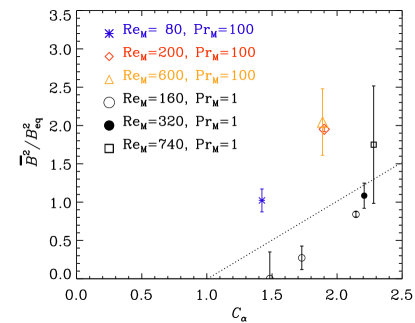
Figure 8: (Color online) Steady state values of $\langle\overline{\bm{B}}^{2}\rangle/B_{\rm eq}^{2}$ as a function of $C_{\alpha}$ for $\mbox{\rm Pr}_{\rm M}=100$ and $\mbox{\rm Pr}_{\rm M}=1$ for $k_{\rm f}/k_{1}=5$ and different values of $\mbox{\rm Re}_{\rm M}$ (different symbols), compared with the theoretical prediction (dotted line).

In Fig. 8 we show results both for $\mbox{\rm Pr}_{\rm M}=100$ and 1. We discuss first runs for $\mbox{\rm Pr}_{\rm M}=100$ at different values of $\epsilon_{\rm f}$ and $\mbox{\rm Re}_{\rm M}$ being either 80, 200, or 600. Most importantly, it turns out that the critical value for LSD onset is not much changed. An extrapolation suggests now $C_{\alpha}^{\rm crit}\approx 0.9$ instead of 1. Furthermore, the dependence of $\langle\overline{\bm{B}}^{2}\rangle/B_{\rm eq}^{2}$ on $C_{\alpha}$ is the same for all three values of $\mbox{\rm Re}_{\rm M}$, and so $C_{\alpha}^{\rm crit}$ is independent of $\mbox{\rm Re}_{\rm M}$. However, the values of $\langle\overline{\bm{B}}^{2}\rangle/B_{\rm eq}^{2}$ are now systematically above the theoretically expected values. This discrepancy with the theory can be easily explained by arguing that the relevant value of $B_{\rm eq}$ has been underestimated in the large $\mbox{\rm Pr}_{\rm M}$ cases. Looking at the power spectrum of the high $\mbox{\rm Pr}_{\rm M}$ simulations in Fig. 9(a), we see that the kinetic energy is indeed subdominant and does not provide a good estimate of the magnetic energy of the small-scale field $\langle\mathchoice{\mbox{\boldmath$\displaystyle b$}}{\mbox{\boldmath$\textstyle b$}}{\mbox{\boldmath$\scriptstyle b$}}{\mbox{\boldmath$\scriptscriptstyle b$}}{}^{2}\rangle/2\mu_{0}$. By contrast, for $\mbox{\rm Pr}_{\rm M}=1$, the magnetic and kinetic energy spectra are similar at all scales except near $k=k_{1}$; see Fig. 9(b). The slight super-equipartition for $k>k_{\rm f}$ is also typical of a SSD [14].

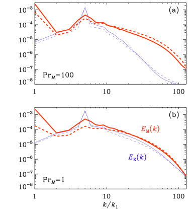
Figure 9: (Color online) Comparison of kinetic and magnetic energy spectra for $\mbox{\rm Pr}_{\rm M}=100$ (upper panel) and $\mbox{\rm Pr}_{\rm M}=1$ (lower panel) for $\sigma=0.2$ (solid lines) and $0.12$ (dashed lines). Magnetic energy spectra are shown as thick red lines while kinetic energy spectra are shown as thin blue lines.

A visualization of the magnetic field for $\mbox{\rm Pr}_{\rm M}=100$ is given in Fig. 10, where we show $B_{x}$ on the periphery of the computational domain. The magnetic field has now clearly strong gradients locally, while still being otherwise dominated by a large-scale component at $k=k_{1}$. In this case the large-scale field shows variations only in the $y$ direction and is of the form

$$\overline{\bm{B}}=(\sin k_{1}y,0,\cos k_{1}y)\,B_{\rm sat}.$$ (24)

This field has negative magnetic helicity, so $\overline{\mbox{\boldmath$J$}}\cdot\overline{\bm{B}}=-k_{1}\overline{\bm{B}}^{2}$, as expected for a forcing function with negative helicity.

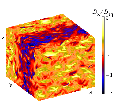
Figure 10: (Color online) Visualization of $B_{x}$ on the periphery of the domain for $\mbox{\rm Pr}_{\rm M}=100$ after resistive saturation.

We have argued that the reason for the larger values in the graph of $\langle\overline{\bm{B}}^{2}\rangle$ versus $C_{\alpha}$ is related to $B_{\rm eq}$ being underestimated for large values of $\mbox{\rm Pr}_{\rm M}$. To confirm this, we now consider calculations with $\mbox{\rm Pr}_{\rm M}=1$, different values of $\epsilon_{\rm f}$ and $\mbox{\rm Re}_{\rm M}$ (from 168 to 745), and fixed scale separation ratio $k_{\rm f}/k_{1}=5$. We see in Fig. 8 that the values are now indeed smaller. An extrapolation would suggest that $C_{\alpha}^{\rm crit}$ is now above 1, but this may not be significant given the uncertainties associated with being so close to the critical value of $\epsilon_{\rm f}$.

LSDs of the type of an $\alpha^{2}$ dynamo only become apparent in the late saturation of the dynamo [15]. This is especially true in the case of large values of $\mbox{\rm Re}_{\rm M}$ when the mean field develops its full strength while the rms value of the small-scale field remains approximately unchanged as $\mbox{\rm Re}_{\rm M}$ increases; see Fig. 11. Note also that the level of fluctuations of both small-scale and large-scale magnetic fields remains approximately similar for different values of $\mbox{\rm Re}_{\rm M}$. This also shows that the emergence of SSD action does not have any noticeable effect on the LSD.

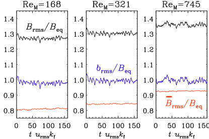
Figure 11: (Color online) Evolution of total magnetic field ($B_{\rm rms}$, upper black line), small-scale magnetic field ($b_{\rm rms}$, blue in the middle), and large-scale magnetic field ($\overline{B}_{\rm rms}$, lower red line) for three values of $\mbox{\rm Re}_{\rm M}$ over a time stretch of 160 turnover times.

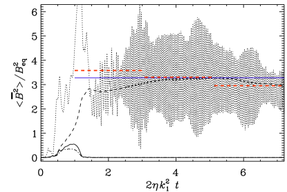
Figure 12: (Color online) Similar to Fig. 1, but for time-dependent ABC-flow driving. As in Fig. 1, we have here $k_{\rm f}/k_{1}=15$ and $\mbox{\rm Re}_{\rm M}\approx 6$.

III.4 ABC-flow forcing

In this paper we have used the fact that the saturation field strength is described by Eq. (16). While this is indeed well obeyed for our randomly driven flows, this does not seem to be the case for turbulence driven by ABC-flow forcing. We demonstrate this by considering a case that is similar to that shown in Fig. 1, where $\mbox{\rm Re}_{\rm M}\approx 6$ in the saturated state. We thus use Eq. (11) with $\sigma=\theta_{0}=1$ and $k_{\rm f}/k_{1}=15$. The kinematic flow velocity reaches an equilibrium rms velocity of $U_{0}=f_{0}/(\nu k_{\rm f}^{2})$. The magnetic Reynolds number based on this velocity is $U_{0}/(\eta k_{\rm f})$, which is chosen to be 13, so that during saturation the resulting value of $\mbox{\rm Re}_{\rm M}$ is about 6, just as in Fig. 1. For the $x$, $y$, and $z$ components we take different forcing frequencies such that $\omega_{i}/(k_{1}U_{0})$ is 10, 11, and 9 for $i=1$, 2, and 3, respectively. These values correspond approximately to the inverse correlation times used in Ref. [11]. The result is shown in Fig. 12. It turns out that the magnetic field grows initially as expected, based on Eq. (21), but then the final saturation phase is cut short below $B_{\rm sat}^{2}/B_{\rm eq}^{2}\approx 3$ rather than the value 12 found with random wave forcing. This is reminiscent of inhomogeneous dynamos in which magnetic helicity fluxes operate. In homogeneous systems, however, magnetic helicity flux divergences have only been seen if there is also shear [39]. In any case, the present behavior is unexpected and suggests that the effective value of $C_{\alpha}$ is reduced. Using the test-field method [40, 41], we have confirmed that the actual value of $C_{\alpha}$ is not reduced. The dynamo is therefore excited, but the value implied for the effective helicity is reduced.

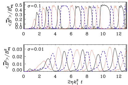
Figure 13: (Color online) Dependence of the normalized $\langle\overline{\bm{B}}^{2}\rangle$ for different planar averages: $yz$ (black), $xz$ (red, dotted), and $xy$ (blue, dashed), for $\sigma=0.1$ (upper panel) and $\sigma=0.01$ (lower panel).

Another possibility is that, especially for small values of $\sigma$, the ABC-flow has nongeneric dynamo properties that emulate aspects of large-scale dynamos. An example is shown in Fig. 13 where we plot the time evolution of all three planar averages ($yz$, $xz$, and $xy$). Even for $\sigma=0.01$, large-scale magnetic fields are still excited, but the field orientation changes periodically on a timescale of 1–2 diffusion times. This is obviously a fascinating topic for further research, but it is unrelated to our main question regarding the minimal helicity of generic turbulent dynamos. It might indeed be an example of so-called incoherent $\alpha$ effect dynamos [42] that have recently attracted increased interest [43, 44, 45].

The main point of this section is to emphasize the limited usefulness of ABC-flow dynamos. Another such example are dynamos driven by the Galloway-Proctor flow, which also has a number of peculiar features; see Ref. [46].

IV Conclusions

In this paper we have studied the simplest possible LSD and have investigated the dependence of its saturation amplitude on the amount of kinetic helicity in the system. We recall that the case of a periodic domain has already been investigated in some detail [29, 47], and that theoretical predictions in the case with shear [16] have been verified numerically for fractional helicities [17]. Yet the issue has now attracted new interest in view of recent results suggesting that, in the limit of large scale separation, the amount of kinetic helicity needed to drive the LSD might actually be much smaller than what earlier calculations have suggested [11]. This was surprising given the earlier confirmations of the theory. As explained above, the reason for the conflicting earlier results may be the fact that the LSD cannot be safely isolated in the linear regime, because it will be dominated by the SSD or, in the case of the ABC-flow dynamo, by some other kind of dynamo that is not due to the $\alpha$ effect. Furthermore, as already alluded to in the introduction, there can be solutions with long-range correlations that could mimic those that are not due to the $\alpha$ effect. Within the framework of the Kazantsev model [21], the solutions to the resulting Schrödinger-type equation can be described as bound states. The addition of kinetic helicity leads to new solutions with long-range correlations as a result of tunneling from the SSD solutions [22, 23, 20]. Indeed, it has been clear for some time that large-scale magnetic fields of the type of an $\alpha^{2}$ dynamo become only apparent in the late saturation of the dynamo [15]. This is especially true for the case of large values of $\mbox{\rm Re}_{\rm M}$ when the mean field develops its full strength while the rms value of the small-scale field due to SSD action remains approximately unchanged as $\mbox{\rm Re}_{\rm M}$ increases; see Fig. 11.

While there will always remain some uncertainty regarding the application to the much more extreme astrophysical parameter regime, we can now rule out the possibility of surprising effects within certain limits of $\mbox{\rm Re}_{\rm M}$ and Re below 740, and scale separation ratios below 80. In stars and galaxies, the scale separation ratio is difficult to estimate, but it is hardly above the largest value considered here. This ratio is largest in the top layers of the solar convection zone where the correlation length of the turbulence is short ($1\,{\rm Mm}$) compared with the spatial extent of the system ($100\,{\rm Mm}$).

Of course, the magnetic Reynolds numbers in the Sun and in galaxies are much larger than what will ever be possible to simulate. Nevertheless, the results presented here show very little dependence of the critical value of $C_{\alpha}$ on $\mbox{\rm Re}_{\rm M}$. For $\mbox{\rm Pr}_{\rm M}=1$, for example, we find $C_{\alpha}^{\rm crit}=1.2$ for $\mbox{\rm Re}_{\rm M}\approx 6$ and $C_{\alpha}^{\rm crit}=1.5$ for $\mbox{\rm Re}_{\rm M}\approx 600$. On the other hand, for larger values of $\mbox{\rm Pr}_{\rm M}$, the value of $C_{\alpha}^{\rm crit}$ can drop below unity ($C_{\alpha}^{\rm crit}=0.9$ for $\mbox{\rm Pr}_{\rm M}=100$). While these changes of $C_{\alpha}^{\rm crit}$ are theoretically not well understood, it seems clear that they are small and do not provide support for an entirely different scaling law, as anticipated in recent work [11].

- [1] E. N. Parker. Cosmical magnetic fields: Their origin and their activity. Oxford, Clarendon Press; New York, Oxford University Press, p. 858, 1979.
- [2] H. K. Moffatt. Magnetic field generation in electrically conducting fluids. Camb. Univ. Press, 1978.
- [3] F. Krause and K.-H. Rädler. Mean-field magnetohydrodynamics and dynamo theory. Oxford, Pergamon Press, Ltd., p. 271, 1980.
- [4] N. Seehafer. Phys. Rev. E, 53:1283–1286, 1996.
- [5] H. Ji. Phys. Rev. Lett., 83:3198–3201, 1999.
- [6] U. Frisch, A. Pouquet, J. Leorat, and A. Mazure. J. Fluid Mech., 68:769–778, 1975.
- [7] E. G. Blackman and G. B. Field. Astrophys. J., 534:984–988, 2000.
- [8] E. G. Blackman and G. B. Field. Month. Not. Roy. Astron. Soc., 318:724–732, 2000.
- [9] N. Kleeorin, D. Moss, I. Rogachevskii, and D. Sokoloff. Astron. Astrophys., 361:L5–L8, 2000.
- [10] A. Brandenburg, S. Candelaresi, and P. Chatterjee. Month. Not. Roy. Astron. Soc., 398:1414–1422, 2009.
- [11] J. Pietarila Graham, E. G. Blackman, P. D. Mininni, and A. Pouquet. Phys. Rev. E, 85:066406, 2012.
- [12] A. Brandenburg. Astrophys. J., 697:1206–1213, 2009.
- [13] A. A. Schekochihin, S. C. Cowley, S. F. Taylor, J. L. Maron, and J. C. McWilliams. Astrophys. J., 612:276–307, 2004.
- [14] N. E. L. Haugen, A. Brandenburg, and W. Dobler. Phys. Rev. E, 70:016308, 2004.
- [15] A. Brandenburg. Astrophys. J., 550:824–840, 2001.
- [16] E. G. Blackman and A. Brandenburg. Astrophys. J., 579:359–373, 2002.
- [17] P. J. Käpylä and A. Brandenburg. Astrophys. J., 699:1059–1066, 2009.
- [18] F. Cattaneo and D. W. Hughes. Month. Not. Roy. Astron. Soc., 395:L48–L51, 2009.
- [19] A. Brandenburg, K.-H. Rädler, M. Rheinhardt, and K. Subramanian. Astrophys. J., 687:L49–L52, 2008.
- [20] S. Boldyrev, F. Cattaneo, and R. Rosner. Phys. Rev. Lett. , 95:255001, 2005.
- [21] A. P. Kazantsev. Sov. J. Exp. Theor. Phys., 26:1031, 1968.
- [22] K. Subramanian. Phys. Rev. Lett. , 83:2957–2960, 1999.
- [23] A. Brandenburg and K. Subramanian. Astron. Astrophys., 361:L33–L36, 2000.
- [24] D. Galloway. Geophys. Astrophys. Fluid Dynam., 106:450–467, 2012.
- [25] B. Galanti, P. L. Sulem, and A. Pouquet. Geophys. Astrophys. Fluid Dynam., 66:183–208, 1992.
- [26] N. Kleeorin, I. Rogachevskii, D. Sokoloff, and D. Tomin. Phys. Rev. E, 79:046302, 2009.
- [27] A. Pouquet, U. Frisch, and J. Léorat. J. Fluid Mech., 77:321–354, 1976.
- [28] K.-H. Rädler and M. Rheinhardt. Geophys. Astrophys. Fluid Dynam., 101:117–154, 2007.
- [29] G. B. Field and E. G. Blackman. Astrophys. J., 572:685–692, 2002.
- [30] A. Brandenburg and K. Subramanian. Astron. Nachr., 328:507, 2007.
- [31] S. Sur, K. Subramanian, and A. Brandenburg. Month. Not. Roy. Astron. Soc., 376:1238–1250, 2007.
- [32] A. Brandenburg, P. J. Käpylä, and A. Mohammed. Phys. Fluids, 16:1020–1027, 2004.
- [33] S. Sur, A. Brandenburg, and K. Subramanian. Month. Not. Roy. Astron. Soc., 385:L15–L19, 2008.
- [34] L. L. Kitchatinov, V. V. Pipin, and G. Ruediger. Astron. Nachr., 315:157–170, 1994.
- [35] I. Rogachevskii and N. Kleeorin. Phys. Rev. E, 64:056307, 2001.
- [36] A. Brandenburg and A. Petrosyan. Astron. Nachr., 333:195, 2012.
- [37] G. K. Batchelor. The Theory of Homogeneous Turbulence. Cambridge: Cambridge University Press, 1953.
- [38] A. Brandenburg. Astron. Nachr., 332:51, 2011.
- [39] A. Hubbard and A. Brandenburg. Astrophys. J., 748:51, 2012.
- [40] M. Schrinner, K.-H. Rädler, D. Schmitt, M. Rheinhardt, and U. R. Christensen. Geophys. Astrophys. Fluid Dynam., 101:81–116, 2007.
- [41] A. Brandenburg, K.-H. Rädler, and M. Schrinner. Astron. Astrophys., 482:739–746, 2008.
- [42] E. T. Vishniac and A. Brandenburg. Astrophys. J., 475:263, 1997.
- [43] M. R. E. Proctor. Month. Not. Roy. Astron. Soc., 382:L39–L42, 2007.
- [44] T. Heinemann, J. C. McWilliams, and A. A. Schekochihin. Phys. Rev. Lett. , 107:255004, 2011.
- [45] D. Mitra and A. Brandenburg. Month. Not. Roy. Astron. Soc., 420:2170–2177, 2012.
- [46] K.-H. Rädler and A. Brandenburg. Month. Not. Roy. Astron. Soc., 393:113–125, 2009.
- [47] K. Subramanian. Bull. Astron. Soc. India, 30:715–721, 2002.