High spatial entanglement via chirped quasi-phase-matched optical parametric down-conversion

Abstract

By making use of the spatial shape of paired photons, parametric down-conversion allows the generation of two-photon entanglement in a multidimensional Hilbert space. How much entanglement can be generated in this way? In principle, the infinite-dimensional nature of the spatial degree of freedom renders unbounded the amount of entanglement available. However, in practice, the specific configuration used, namely its geometry, the length of the nonlinear crystal and the size of the pump beam, can severely limit the value that could be achieved. Here we show that the use of quasi-phase-matching engineering allows to increase the amount of entanglement generated, reaching values of tens of ebits of entropy of entanglement under different conditions. Our work thus opens a way to fulfill the promise of generating massive spatial entanglement under a diverse variety of circumstances, some more favorable for its experimental implementation.

I Introduction

Entanglement is a genuine quantum correlation between two or more parties, with no analogue in classical physics. During last decades it has been recognized as a fundamental tool in several quantum information protocols, such as quantum teleportation bennett1993 , quantum cryptography ekert1991 and quantum key distribution ribordy2000 , and distributed quantum computing serafini2006 .

Nowadays, spontaneous parametric down-conversion (SPDC), a process where the interaction of a strong pump beam with a nonlinear crystal mediates the emission of two lower-frequency photons (signal and idler), is a very convenient way to generate photonic entanglement torres2011 . Photons generated in SPDC can exhibit entanglement in the polarization degree of freedom kwiat1995 , frequency law2000 and spatial shape barbosa2000 ; mair2000 . One can also make use of a combination of several degrees of freedom barreiro2005 ; nagali2009 .

Two-photon entanglement in the polarization degree of freedom is undoubtedly the most common type of generated entanglement, due both to its simplicity, and that it suffices to demonstrate a myriad of important quantum information applications. But the amount of entanglement is restricted to $1$ ebit of entropy of entanglement comment1 , since each photon of the pair can be generally described by the superposition of two orthogonal polarizations (two-dimensional Hilbert space). On the other hand, frequency and spatial entanglement occurs in an infinite dimensional Hilbert space, offering thus the possibility to implement entanglement that inherently lives in a higher dimensional Hilbert space (qudits).

Entangling systems in higher dimensional systems (frequency and spatial degrees of freedom) is important both for fundamental and applied reasons. For example, noise and decoherence tend to degrade quickly quantum correlations. However, theoretical investigations predict that physical systems with increasing dimensions can maintain non-classical correlations in the presence of more hostile noise kaszlikowski2000 ; collins2002 . Higher dimensional states can also exhibit unique outstanding features. The potential of higher-dimensional quantum systems for practical applications is clearly illustrated in the demonstration of the so-called quantum coin tossing, where the power of higher dimensional spaces is clearly visible molina2005 .

The amount of spatial entanglement generated depends of the SPDC geometry used (collinear vs non-collinear), the length of the nonlinear crystal ($L$) and the size of the pump beam ($w_{0}$). To obtain an initial estimate, let us consider a collinear SPDC geometry. Under certain approximations aprox , the entropy of entanglement can be calculated analytically. Its value can be shown to depend on the ratio $L/L_{d}$, where $L_{d}=k_{p}w_{0}^{2}/2$ is the Rayleigh range of the pump beam and $k_{p}$ is its longitudinal wavenumber. Therefore, large values of the pump beam waist $w_{0}$ and short crystals are ingredients for generating high entanglement oemrawsingh2005 . However, the use of shorter crystals also reduce the total flux-rate of generated entangled photon pairs. Moreover, certain applications might benefit from the use of focused pump beams. For instance, for a $L=1$ mm long stoichiometric lithium tantalate (SLT) crystal, with pump beam waist $w_{0}=100$ $\mu$m, pump wavelength $\lambda_{p}=400$ nm and extraordinary refractive index $n_{e}(\lambda_{p})=2.27857$ bruner2003 , one obtains $E\sim 8.5$ aprox . For a longer crystal of $L=20$ mm, the amount of entanglement is severely reduced to $E\sim 4.2$ ebits.

We put forward here a scheme to generate massive spatial entanglement, i. e., an staggering large value of the entropy of entanglement, independently of some relevant experimental parameters such as the crystal length or the pump beam waist. This would allow to reach even larger amounts of entanglement that possible nowadays with the usual configurations used, or to attain the same amount of entanglement but with other values of the nonlinear crystal length or the pump beam waist better suited for specific experiments.

Our approach is based on a scheme originally used to increase the bandwidth of parametric down-conversion carrasco2004 ; nasr2008 ; svozilik2009 . A schematic view of the SPDC configuration is shown in Fig.1. It makes use of chirped quasi-phase-matching (QPM) gratings with a linearly varying spatial frequency given by $K_{g}(z)=K_{0}-\alpha(z+L/2)$, where $K_{0}$ is the grating’s spatial frequency at its entrance face ($z=-L/2$), and $\alpha$ is a parameter that represents the degree of linear chirp. The period of the grating at distance $z$ is $p(z)=2\pi/K_{g}(z)$, so that the parameter $\alpha$ writes

$$\alpha=\frac{2\pi}{L}\frac{p_{f}-p_{i}}{p_{f}p_{i}}$$ (1)

where $p_{i}$ is the period at the entrance face of the crystal, and $p_{f}$ at its output face.

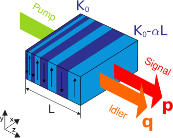
Figure 1: Scheme of SPDC in a linearly chirped quasi-phase-matched nonlinear crystal. The pump beam is a Gaussian beam, and ${\bf p}$ and ${\bf q}$ designate the transverse wave numbers of the signal and idler photons, respectively. $K_{0}$ is the grating wave-vector at the input face of the nonlinear crystal, and $K_{0}-\alpha L$ at its output face. The signal and idler photons can have different polarizations or frequencies. The different colors (or different direction of arrows) represent domains with different sign of the nonlinear coefficient.

The key idea is that at different points along the nonlinear crystal, signal and idler photons with different frequencies and transverse wavenumbers can be generated, since the continuous change of the period of the QPM gratings allows the fulfillment of the phase-matching conditions for different frequencies and transverse wavenumbers. If appropriately designed narrow-band interference filters allow to neglect the frequency degree of freedom of the two-photon state, the linearly chirped QPM grating enhance only the number of spatial modes generated, leading to a corresponding enhancement of the amount of generated spatial entanglement.

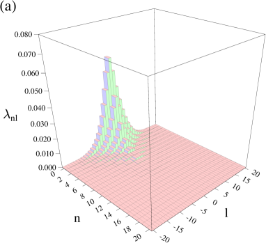
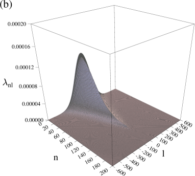
Figure 2: Weight of the Schmidt coefficients $\lambda_{nl}$ for (a) $\alpha=0\;\mu m^{-2}$ and (b) $\alpha=10\times 10^{-6}\;\mu m^{-2}$. The nonlinear crystal length is $L=20$ mm and the pump beam waist is $w_{0}=100\;\mu m$.

II Theoretical model

In order to determine how much spatial entanglement can be generated in SPDC with the use of chirped QPM, let us consider a nonlinear optical crystal illuminated by a quasi-monochromatic laser Gaussian pump beam of waist $w_{0}$. Under conditions of collinear propagation of the pump, signal and idler photons with no Poynting vector walk-off, which would be the case of a noncritical type-II quasi-phase matched configuration, the amplitude of the quantum state of the generated two-photon pair generated in SPDC reads in transverse wavenumber space

$$|\Psi\rangle=\int d{\bf p}d{\bf q}\Psi\left({\bf p},{\bf q}\right)|{\bf p}\rangle_{s}|{\bf q}\rangle_{i},$$ (2)

where ${\bf p}$ ($\bf q$) is the transverse wavenumber of the signal (idler) photon. $\Psi$ is the joint amplitude of the two-photon state, so that $|\Psi\left({\bf p},{\bf q}\right)|^{2}$ is the probability to detect a signal photon with transverse wave-number ${\bf p}$ in coincidence with an idler photons with ${\bf q}$.

The joint amplitude that describes the quantum state of the paired photons generated in a linearly chirped QPM crystal, using the paraxial approximation, is equal to

$$\Psi\left({\bf p},{\bf q}\right) = C\exp\left(-\frac{w^{2}_{0}}{4}|\mathbf{p+q}|^{2}\right)$$

$$\times \int_{-L/2}^{L/2}dz\exp\left[i\frac{|\mathbf{p}-\mathbf{q}|^{2}}{2k_{p}}z+i\alpha\left(z+\frac{L}{2}\right)z\right],$$

where $C$ is a normalization constant ensuring $\int d\mathbf{q}\int d\mathbf{p}|\Psi\left(\mathbf{p},\mathbf{q}\right)|^{2}=1$. Notice that the value of $K_{0}=2\pi/p(-L/2)$ does now show up in Eq. (II), since we make use of the fact that there is phase matching for ${\bf p}={\bf q}=0$ at certain location inside the nonlinear crystal, which in our case it turns out to be the input face ($z=-L/2$).

After integration along the z-axis one obtains

$$\Psi(\mathbf{p},\mathbf{q}) = C\sqrt{\frac{i\pi}{4\alpha}}exp\left[-\frac{w_{0}^{2}}{4}|\mathbf{p}+\mathbf{q}|^{2}-i\left(\frac{\alpha L^{2}}{16}+\frac{L|\mathbf{p}-\mathbf{q}|^{2}}{8k_{p}}+\frac{\mathbf{|p-}\mathbf{q}|^{4}}{16\alpha k_{p}^{2}}\right)\right]$$ (4)

$$\times\left[\mathrm{erf}\left(\frac{3\sqrt{\alpha}L}{4\sqrt{i}}+\frac{|\mathbf{p}-\mathbf{q}|^{2}}{4k_{p}\sqrt{i\alpha}}\right)-\mathrm{erf}\left(-\frac{\sqrt{\alpha}L}{4\sqrt{i}}+\frac{|\mathbf{p}-\mathbf{q}|^{2}}{4k_{p}\sqrt{i\alpha}}\right)\right],$$

where $\mathrm{erf}$ refers to the error function. Notice that Eq. (4) is similar to the one describing the joint spectrum of photon pairs in the frequency domain, when the spatial degree of freedom is omitted nasr2008 ; svozilik2009 . The reason is that both equations originate in phase matching conditions along the propagation direction ($z$ axis).

Since all the configuration parameters that define the down conversion process show rotational symmetry along the propagation direction $z$, the joint amplitude given by Eq. (4) can be written as

$$\Psi\left(\mathbf{p},\mathbf{q}\right)=\sum^{\infty}_{l=-\infty}B_{l}\left(p,q\right)e^{il\left(\varphi_{p}-\varphi_{q}\right)}.$$ (5)

Here, we have made use of polar coordinates in the transverse wave-vector domain for the signal, $\mathbf{p}=\left(p\cos\varphi_{p},p\sin\varphi_{p}\right)$, and idler photons $\mathbf{q}=\left(q\cos\varphi_{q},q\sin\varphi_{q}\right)$, where $\varphi_{p,q}$ are the corresponding azimuthal angles, and $p,q$ are the radial coordinates. The specific dependence of the Schmidt decomposition on the azimuthal variables $\varphi_{p}$ and $\varphi_{p}$ reflects the conservation of orbital angular momentum in this SPDC configuration osorio2008 , so that a signal photon with OAM winding number $+l$ is always accompanied by a corresponding idler photon with OAM winding number $-l$. The probability of such coincidence detection for each value of $l$ is the spiral spectrum torres2003 of the two-photon state, i.e., the set of values $P_{l}=\int pdp\,qdq\,|B_{l}(p,q)|^{2}$. Recently, the spiral spectrum of some selected SPDC configuration have been measured pires2010 .

The Schmidt decomposition ekert1995 ; law2005 of the spiral function, i.e., $B_{l}(p,q)=\sum_{n=0}^{\infty}\sqrt{\lambda_{nl}}f_{nl}(p)g_{nl}(q)$, is the tool to quantify the amount of entanglement present. $\lambda_{nl}$ are the Schmidt coefficients (eigenvalues), and the modes $f_{nl}$ and $g_{nl}$ are the Schmidt modes (eigenvectors). Here we obtain the Schmidt decomposition by means of a singular-value decomposition method. Once the Schmidt coefficients are obtained, one can obtain the entropy of entanglement as $E=-\sum_{nl}\lambda_{nl}\log_{2}\lambda_{nl}$. An estimation of the overall number of spatial modes generated is obtained via the Schmidt number $K=1/\sum_{nl}\lambda_{nl}^{2}$, which can be interpreted as a measure of the effective dimensionality of the system. Finally, the spiral spectrum is obtained as $P_{l}=\sum_{n}\lambda_{nl}$.

III Discussion

For the sake of comparison, let us consider first the usual case of a QPM SLT crystal with no chirp, i.e., $\alpha=\,0\,\mu m^{-2}$, and length $L=20$ mm, pumped by a Gaussian beam with beam waist $w_{0}=\,100\,\mu m$ and wavelength $\lambda_{p}=400$ nm. In this case, the integration of Eq. (II) leads to walborn2003

$$\Psi(\mathbf{p},\mathbf{q})=C\exp{\left(-\frac{w^{2}_{0}}{4}|\mathbf{p}+\mathbf{q}|^{2}\right)}\mathrm{sinc}\left(\frac{L|\mathbf{p}-\mathbf{q}|^{2}}{4k_{p}}\right).$$ (6)

The Schmidt coefficients are plotted in Fig. 2(a), and the corresponding spiral spectrum is shown in Fig. 3(a). The main contribution to the spiral spectrum comes from the spatial modes with $l=0$. The entropy of entanglement for this case is $E=6.4$ ebits and the Schmidt number is $K=42.9$.

Nonzero values of the chirp parameter $\alpha$ lead to an increase of number of generated modes, as it can be readily seen in Fig. 2(b) for $\alpha\,=10\times 10^{-6}$ $\mu m^{-2}$ and $w_{0}\,=100$ $\mu$m. This broadening effect is also reflected in the corresponding broadening of spiral spectrum, as shown in Fig. 3(b). Indeed, Fig. 4(a) shows that the entropy of entanglement increases with increasingly larger values of the chirping parameter, even though for a given value of $w_{0}$, its increase saturates for large values of $\alpha$. For $w_{0}=\,300\,\mu m$ and $\alpha\,=10\times 10^{-6}\,\mu m^{-2}$, we reach a value of $E=16.6$ ebits. On the contrary, the Schmidt number $K$ rises linearly with $\alpha$, as can be observed in Fig. 4(b), for all values of $w_{0}$. For sufficiently large values of $w_{0}$ and $\alpha$, $K$ reaches values of several thousands of spatial modes, i.e. $K=87113$ for the same $w_{0}$ and $\alpha$. For large values of $E$, a further increase of $E$ requires an even much larger increase of the number of spatial modes involved, which explain why an increase of the number of modes involved only produces a modest increase of the entropy of entanglement. Notice that the spiral spectrum presented in Fig. 3(b) is discrete. Notwithstanding, it might look continuous since it is the result from the presence of several hundreds of OAM modes with slightly decreasing weights.

Figure 3: The spiral spectrum $P_{l}$ for (a) $\alpha=0\;\mu m^{-2}$ and (b) $\alpha=10\times 10^{-6}\;\mu m^{-2}$. The nonlinear crystal length is $L=20$ mm and the pump beam waist is $w_{0}=100\;\mu m$.

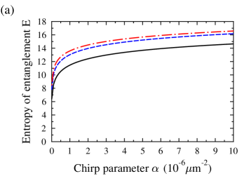
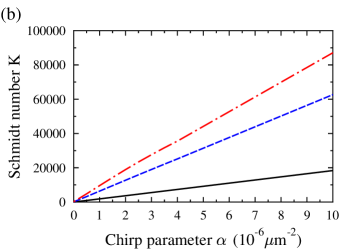
Figure 4: (a) The entropy of entanglement $E$ and (b) the Schmidt number $K$ as a function of the chirp parameter $\alpha$ for $w_{0}=100\;\mu m$ (solid black line), $w_{0}=200\;\mu m$ (dashed blue line) and $w_{0}=300\;\mu m$ (dotted-and-dashed red line).

We have discussed entanglement in terms of transverse modes which arise from the Schmidt decomposition of the two-photon amplitude and, as such, they attain appreciable values in the whole transverse plane. Alternatively, the existing spatial correlations between the signal and idler photons can also be discussed using second-order intensity correlation functions Hamar2010 . In this approach, correlations are quantified by the size of the correlated area ($\Delta{\bf p}$) where it is highly probable to detect a signal photon provided that its idler twin has been detected with a fixed transverse wave vector ${\bf q}$. We note that the azimuthal width of correlated area decreases with the increasing width of the distribution of Schmidt eigenvalues along the OAM winding number $l$. On the other hand, the increasing width of the distribution of Schmidt eigenvalues along the remaining number $n$ results in a narrower radial extension of the correlated area. An increase in the number of modes $K$ results in a diminishing correlation area, both in the radial and azimuthal directions. The correlated area drops to zero in the limit of plane-wave pumping, where attains the form of a $\delta$ function. The use of such correlations in parallel processing of information represents the easiest way for the exploitation of massively multi-mode character of the generated beams.

For the sake of comparison, when considering frequency entanglement, the entropy of entanglement depends on the ratio between the bandwidth of the pump beam (typically $B_{p}\sim 5$ MHz) and the bandwidth of the down-converted two-photon state ($B_{dc}$) parker2000 ; PerinaJr2008 . For type II SPDC, one has typically values of $E\sim 1-2$ law2000 . Increasing the bandwidth of the two-photon state, one can reach values of $B_{dc}>1000$ THz, therefore allowing typical ratios greater than $B_{dc}/B_{p}\gg 10^{8}$, with $E>25$ martin2009 .

IV Conclusion

In conclusion, we have presented a new way to increase significantly the amount of two-photon spatial entanglement generated in SPDC by means of the use of chirped quasi-phase-matching nonlinear crystals. This opens the door to the generation of high entanglement under various experimental conditions, such as different crystal lengths and sizes of the pump beam.

QPM engineering can also be an enabling tool to generate truly massive spatial entanglement, with state of the art QPM technologies nasr2008 potentially allowing to reach entropies of entanglement of tens of ebits. Therefore, the promise of reaching extremely high degrees of entanglement, offered by the use of the spatial degree of freedom, can be fulfilled with the scheme put forward here. The experimental tools required are available nowadays. The use of extremely high degrees of spatial entanglement, as consider here, would demand the implementation of high aperture optical systems. For instance, for a spatial bandwidth of $\Delta{\bf p}\sim 2\mu m^{-1}$, the aperture required for $\lambda_{p}=400$ nm is $\Delta\theta\sim 4^{\circ}-6^{\circ}$.

The shaping of QPM gratings are commonly used in the area of non-linear optics for multiple applications such as beam and pulse shaping, harmonic generation and all-optical processing hum2007 . In the realm of quantum optics, its uses are not so widespread, even though QPM engineering has been considered, and experimentally demonstrated, as a tool for spatial qpm2004 ; yu2008 and frequency nasr2008 control of entangled photons. In view of the results obtained here concerning the enhancement of the degree of spatial entanglement, it could be possible to devise new types of gratings that turn out to be beneficial for other applications in the area of quantum optics.

This work was supported by the Government of Spain (Project FIS2010-14831) and the European union (Project PHORBITECH, FET-Open 255914). J. S. thanks the project FI-DGR 2011 of the Catalan Government. This work has also supported in part by projects COST OC 09026, CZ.1.05/2.1.00/03.0058 of the Ministry of Education, Youth and Sports of the Czech Republic and by project PrF-2012-003 of Palacký University.

References

- (1) C. H. Bennett, G. Brassard, C. Crépeau, R. Jozsa, A. Peres, and W. K. Wootters, Phys. Rev. Lett. 70, 1895 (1993).
- (2) A. K. Ekert, Phys. Rev. Lett. 67, 661 (1991).
- (3) G. Ribordy, J. Brendel, J. D. Gautier, N. Gisin, and H. Zbinden, Phys. Rev. A 63, 012309 (2000).
- (4) A. Serafini, S. Mancini, and S. Bose, Phys. Rev. Lett. 96, 010503 (2006).
- (5) J. P. Torres, K. Banaszek and I. A. Walmsley, Progress in Optics 56 (chapter V), 227 (2011).
- (6) P. G. Kwiat, K. Mattle, H. Weinfurter, A. Zeilinger, A. V. Sergienko, and Y. Shih, Phys. Rev. Lett. 75, 4337 (1995).
- (7) C. K. Law, I. A. Walmsley, and J. H. Eberly, Phys. Rev. Lett. 84, 5304 (2000).
- (8) H. H. Arnaut and G. A. Barbosa, Phys. Rev. Lett. 85, 286 (2000).
- (9) A. Mair, A. Vaziri, G. Weihs and A. Zeilinger, Nature 412, 313 (2001).
- (10) J. T. Barreiro, N. K. Langford, N. A. Peters, and P. G. Kwiat, Phys. Rev. Lett. 95, 260501 (2005).
- (11) E. Nagali, F. Sciarrino, F. De Martini, L. Marrucci, B. Piccirillo, E. Karimi and E. Santamato, Phys. Rev. Lett. 103, 013601 (2009).
- (12) For a two-photon state with density matrix , the entropy of entanglement is defined as , where is the partial trace over the variables describing subsystem of the global density matrix. The entropy of entanglement of a maximally entangled quantum state, whose two parties live in a -dimensional system, is . Since the state of polarization of a single photon is a two-dimensional system, the maximum entropy of entanglement is .
- (13) D. Kaszlikowski, P. Gnacinski, M. Zukowski, W. Miklaszewski, and A. Zeilinger, Phys. Rev. Lett. 85, 4418 (2000).
- (14) D. Collins, N. Gisin, N. Linden, S. Massar, and S. Popescu, Phys. Rev. Lett. 88, 040404 (2002).
- (15) G. Molina-Terriza, A. Vaziri, R. Ursin and A. Zeilinger, Phys. Rev. Lett. 94, 040501 (2005).
- (16) The approximation consist of substituting the sinc function appearing later on in Eq. (6) by a Gaussian function, i.e. with , so that both functions coincide at the -intensity. For a detailed calculation, see K. W. Chan, J. P. Torres, and J. H. Eberly, Phys. Rev. A 75, 050101(R) (2007).
- (17) S. S. R. Oemrawsingh, X. Ma, D. Voigt, A. Aiello, E. R. Eliel, G. W. ’t Hooft, and J. P. Woerdman, Phys. Rev. Lett. 95, 240501 (2005).
- (18) A. Bruner, D. Eger, M. B. Oron, P. Blau, M. Katz, and S. Ruschin, Opt. Lett. 28, 194 (2003).
- (19) S. Carrasco, J. P. Torres, L. Torner, A. Sergienko, B. E. A. Saleh, and M. C. Teich, Opt. Lett. 29, 2429 (2004).
- (20) M. B. Nasr, S. Carrasco, B. E. A. Saleh, A. V. Sergienko, M. C. Teich, J. P. Torres, L. Torner, D. S. Hum, and M. M. Fejer, Phys. Rev. Lett. 100, 183601 (2008).
- (21) J. Svozilík, and J. Peřina Jr., Phys. Rev. A 80, 023819 (2009).
- (22) C. I. Osorio, G. Molina-Terriza, and J. P. Torres, Phys. Rev. A 77, 015810 (2008).
- (23) J. P. Torres, A. Alexandrescu, and L. Torner, Phys. Rev. A 68, 050301 (2003).
- (24) H. Di Lorenzo Pires, H. C. B. Florijn, and M. P. van Exter, Phys. Rev. Lett. 104, 020505 (2010).
- (25) A. Ekert and P. L. Knight, Am. J. Phys. 63, 415 (1995).
- (26) C. K. Law and J. H. Eberly, Phys. Rev. Lett. 92, 127903 (2004).
- (27) S.P. Walborn, A.N. de Oliveira, S. Padua, and C.H. Monken, Phys. Rev. Lett 90, 143601 (2003)
- (28) S. Parker, S. Bose, and M. B. Plenio, Phys. Rev. A 61, 032305 (2000).
- (29) M. Hamar, J. Peřina Jr., O. Haderka, and V. Michálek, Phys. Rev. A 81, 043827 (2010).
- (30) J. Peřina Jr., Phys. Rev. A 77, 013803 (2008).
- (31) M. Hendrych, X. Shi, A. Valencia, and J. P. Torres, Phys. Rev. A 79, 023817 (2009).
- (32) D. S. Hum and M. M. Fejer, C. R. Physique 8, 180 (2007).
- (33) J. P. Torres, A. Alexandrescu, S. Carrasco, and L. Torner, Opt. Lett. 29, 376 (2004).
- (34) X. Q. Yu, P. Xu, Z. D. Xie, J. F. Wang, H.Y. Leng, J. S. Zhao, S. N. Zhu, and N. B. Ming, Phys. Rev. Lett. 101, 233601 (2008).