Effective Rheology of Bubbles Moving in a Capillary Tube

Abstract

We calculate the average volumetric flux versus pressure drop of bubbles moving in a single capillary tube with varying diameter, finding a square-root relation from mapping the flow equations onto that of a driven overdamped pendulum. The calculation is based on a derivation of the equation of motion of a bubble train from considering the capillary forces and the entropy production associated with the viscous flow. We also calculate the configurational probability of the positions of the bubbles.

Multiphase flow in porous media plays a pivotal role in a vast range of applications in different fields such as oil recovery, soil mechanics and hydrology d79 ; b88 ; a92 ; s95 . In spite of its relevance in these important fields, fundamental questions still linger on. In particular, this is true in connection with steady-state multiphase flow gr93 ; ap95 ; ap99 ; kah02 ; kh02 ; tkrlmtf09 ; tlkrfm09 , which sets in after the initial instabilities such as viscous fingering are over in e.g. flooding experiments. A way to study this flow in the laboratory, is to simultaneously inject the two immiscible fluids into the porous medium and let them mix until a steady state where clusters and bubbles break up and merge but in such a way that their averages remain constant tkrlmtf09 ; tlkrfm09 .

Recently, the relation between average volumetric flow and excess pressure drop across the system has been investigated both experimentally and theoretically tkrlmtf09 ; tlkrfm09 ; rcs11 ; sh12 . The conclusion from these studies is that the volumetric flux depends quadratically on the excess pressure. This is in contrast to the assumptions of linearity commonly made when considering such systems, e.g. in connection with invoking the concepts of relative permeability in reservoir simulations at the flow rates where capillary and viscous forces compete c06 .

One aim of this work is to derive the volumetric flux versus excess pressure drop for a single capillary tube. We find that there is a square root singularity in this relation. This is in contrast to a the situation for network of pores, i.e., a porous medium. We base this calculation on the equation of motion of a bubble train in a long capillary tube with varying diameter, the Washburn equation w21 . We derive this equation following a different route than the now 91 year old original derivation. Lastly, we derive the probability distribution of the configuration of bubbles in the tube. This makes it possible to calculate the average of any quantity associated with the flow.

We assume a long tube of length $L$ oriented along an $x$ axis. The radius of the tube, $r$, varies with the position along the tube as

$$r=\frac{r_{0}}{1-a\cos\left(2\pi x/l\right)}\;,$$ (1)

where $r_{0}$ is the average radius of the tube, $l$ is the wavelength along the tube and $a$ is the dimensionless amplitude of the oscillation, see Fig. 1. We assume $L\gg l$.

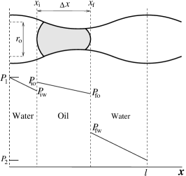
Figure 1: Shape of tube and corresponding pressure drops.

We now imagine a bubble in a tube segment with length $l$ limited by interfaces at $x_{i}$ and $x_{f}$. The fluid in the bubble (“oil”) is less wetting with respect to the tube walls than the fluid outside the bubble (“water”).

The capillary pressure drop across the interface between the two fluids at $x_{i}$ is b88

$$\frac{2\sigma_{wo}}{r(x_{i})}=\frac{2\sigma_{wo}}{r_{0}}\ \left[1-a\cos\left(\frac{2\pi x_{i}}{l}\right)\right]\;,$$ (2)

and across the interface at $x_{f}$,

$$-\frac{2\sigma_{wo}}{r(x_{f})}=-\frac{2\sigma_{wo}}{r_{0}}\ \left[1-a\cos\left(\frac{2\pi x_{f}}{l}\right)\right]\;.$$ (3)

Here, $\sigma_{wo}$ is the surface tension between the two fluids. We sum the two capillary pressure drops to get

$$p_{c}(x_{b})=\frac{4\sigma_{wo}a}{r_{0}}\ \sin\left(\frac{\pi\Delta x_{b}}{l}\right)\ \sin\left(\frac{2\pi x_{b}}{l}\right)\;,$$ (4)

where we have defined $x_{b}=(x_{i}+x_{f})/2$ and $\Delta x_{b}=x_{f}-x_{i}$. We assume the length of the bubble $\Delta x_{b}$ to be smaller than the wavelength $l$, which is also equal to the length of the tube segment. Furthermore we have chosen the origin of the $x$-coordinate such the whole bubble is located between 0 and $l$.

We assume the viscosities of the two fluids to be $\mu_{w}$ (“water”) and $\mu_{o}$ (“oil”) respectively. In order to derive a constitutive equation between volumetric flux $q$ and pressure drop along the tube, $\Delta P=(L/l)\Delta p$, we consider the entropy production of a tube segment with an average cross-sectional area $\pi r_{0}^{2}$ and length $l$ kbjg10 ,

$$\frac{dS}{dt}=\int_{0}^{l}dx\ \dot{s}(x)\;,$$ (5)

where $\dot{s}(x)$ the entropy production in the tube per unit of length at position $x$. We assume the temperature to be constant along the tube. The entropy production in the fluid sections times the temperature is equal to $-q\partial p(x)/\partial x$, where $q$ is the volumetric flux and $p(x)$ the pressure at $x$. Because of the incompressible nature of the flow, the volumetric flux is independent of position. There is no excess entropy production at the interfaces between the fluid and the bubble, assuming equilibrium between the two immiscible fluids, cf. Eqs. (2) and (3). Substituting $\dot{s}(x)$ into Eq. (5) and integrating gives

$$\Theta\frac{dS}{dt} = -q\left(p_{iw}-p_{1}\right)-q\left(p_{fo}-p_{io}\right)-q\left(p_{2}-p_{fw}\right)$$ (7)

$$= -q\left(\Delta p-p_{c}(x_{b})\right)$$

where $\Theta$ is the temperature, $\Delta p=p_{2}-p_{1}$ is the pressure drop across a length $l$ and $p_{c}(x_{b})=p_{io}-p_{iw}+p_{fw}-p_{fo}$ is the capillary pressure difference given in Eq. (4). The resulting linear force-flux relations for the pressure differences in the three sections are written in the form

$$p_{iw}-p_{1} = -R_{w}x_{i}q$$

$$p_{fo}-p_{io} = -R_{o}\Delta x_{b}q$$

$$p_{2}-p_{fw} = -R_{w}\left(l-x_{f}\right)q$$ (8)

where $R_{w}$ and $R_{o}$ are the Onsager resistivities per unit of length for the flow of water and bubble phases, respectively. Using Poisseulle flow the Onsager resistivities are equal to $8\mu/(\pi r_{0}^{4})$, where $\mu$ is the viscosity of the fluid considered. The resulting pressure differences are

$$p_{iw}-p_{1} = -\frac{8}{\pi r_{0}^{4}}x_{i}\mu_{w}q$$

$$p_{fo}-p_{io} = -\frac{8}{\pi r_{0}^{4}}\Delta x_{b}\mu_{o}q$$

$$p_{2}-p_{fw} = -\frac{8}{\pi r_{0}^{4}}\left(l-x_{f}\right)\mu_{w}q$$ (9)

The sum of the pressure differences gives the constitutive equation for motion of a single bubble

$$q=-\frac{\pi r_{0}^{4}}{8\mu_{av}l}\ \left(\Delta p-p_{c}(x_{b})\right)\;.$$ (10)

where

$$\mu_{av}=\frac{1}{l}\ \left[\left(l-\Delta x_{b}\right)\mu_{w}+\Delta x_{b}\mu_{o}\right]$$ (11)

is the average viscosity of the two fluids, which we note is independent of the position of the bubble. One may obtain a similar expression directly from Eq. (7). Eqs. (10) and (11) were first derived by Washburn w21 , but by a different route. The present procedure clarifies why Eq. (10) should contain the average viscosity and how the contribution due to the capillary pressure arises.

The center of mass coordinate of the bubble moves as $\pi r_{0}^{2}\dot{x}_{b}=q$. Hence, we have the equation of motion

$$\dot{x}_{b}=-\frac{r_{0}^{2}}{8l\mu_{av}}\left[\Delta p-\gamma\sin\left(\frac{2\pi x_{b}}{l}\right)\right]\;,$$ (12)

where we have defined

$$\gamma=\frac{4\sigma a}{r_{0}}\ \sin\left(\frac{\pi\Delta x_{b}}{l}\right)\;.$$ (13)

We introduce the angle variable $\theta=2\pi x_{b}/l$ and the time scale $\tau=\gamma t\pi r_{0}^{2}/(4l^{2}\mu_{av})$. We assume the pressure drop to be negative, $\Delta p=-|\Delta p|$. The equation of motion (13) then becomes

$$\frac{d\theta}{d\tau}=\frac{|\Delta p|}{\gamma}+\sin\theta\;,$$ (14)

which is nothing but the equation of motion for the overdamped driven pendulum s94 .

The period $T_{\tau}$ (measured in the same units as $\tau$), needed for the bubble to move from one end of the tube with length $l$ to the other end for a given $\Delta p$, is

$$T_{\tau}=\int_{0}^{T_{\tau}}d\tau=\int_{0}^{2\pi}\frac{d\theta}{d\theta/d\tau}=\frac{2\pi\gamma}{\sqrt{\Delta p^{2}-\gamma^{2}}}\;,$$ (15)

In seconds this time is

$$T=\frac{4l^{2}\mu_{av}}{\gamma\pi r_{0}^{2}}T_{\tau}=\frac{8l^{2}\mu_{av}}{r_{0}^{2}\sqrt{\Delta p^{2}-\gamma^{2}}}\;.$$ (16)

We then define the time-averaged angular speed as

$$\langle\frac{d\theta}{d\tau}\rangle = \frac{1}{T_{\tau}}\int_{0}^{T_{\tau}}\frac{d\theta}{d\tau}d\tau=\frac{1}{T_{\tau}}\int_{0}^{2\pi}d\theta$$ (17)

$$= \frac{2\pi}{T_{\tau}}=\frac{1}{\gamma}\ \sqrt{\Delta p^{2}-\gamma^{2}}\;.$$

Now, transforming back from $d\theta/d\tau$ to $\dot{x}_{b}$ to volumetric flux, $q$, we find the time-averaged flux equation

$$\langle q\rangle=-\frac{\pi r_{0}^{4}}{8\mu_{av}l}\mathrm{sgn}(\Delta p)\Theta(|\Delta p|-\gamma)\sqrt{\Delta p^{2}-\gamma^{2}}\;,$$ (18)

where $\mathrm{sgn}$ is the sign function and $\Theta$ is the Heaviside function. Hence, for $|\Delta p|<\gamma$ there is no flow through the tube. Furthermore, if there is flow, $T\langle\dot{x}_{b}\rangle=l$, as one would expect.

We see that we can write Darcy’s law for the time averaged volume flux only if $\gamma=0$, which is the case if the tube has a constant radius ($a=0$). The deviation from this law for the time average is due to a capillary pressure which varies as a function of the position of the bubble along the tube. The effective flux equation (18) has a threshold pressure that must be overcome to induce flow, $\gamma$ defined in Eq. (13). Close to this threshold, when $|\Delta p|-\gamma\ll\gamma$, the average flow equation becomes

$$\langle q\rangle=-\frac{\pi r_{0}^{4}}{8\mu_{av}l}\sqrt{2\gamma}\mathrm{sgn}(\Delta p)\Theta(|\Delta p|-\gamma)\sqrt{|\Delta p|-\gamma}\;,$$ (19)

i.e., there is a square root singularity. As shown in Ref. s94 , this square root is a consequence of the quadratic extremum of $r$ in Eq. (1) leading to a saddle-node bifurcation, and therefore it does not depend on the specific sinusoidal shape of the profile chosen. The smaller the value of $r_{0},$ the larger is the threshold value. A radius of 10 micrometer can give a threshold of the order of 80 bar, which is non-negligible for most practical purposes.

We may generalize these considerations to a tube segment with length $L=\left(2N+1\right)l$ in which there are $2N+1$ bubbles numbered from $-N$ to $N$. Each bubble $j$ may be characterized by a center of mass position $x_{j}$ and a width $\Delta x_{j}$. In view of the incompressible nature of the flow the volume flux $q$ is independent of the position. This implies that the velocity $\dot{x_{j}}$ of all the bubbles is the same, $\dot{x_{0}}=\dot{x_{j}}$. The equation of motion (12) may then be generalized as follows,

$$\dot{x_{0}}=-\frac{r_{0}^{2}}{8L\mu_{av}}\left[\Delta P-\sum_{j=-N}^{+N}\gamma_{i}\sin\left(\frac{2\pi}{l}(x_{0}+\delta x_{j})\right)\right]\;,$$ (20)

where $\Delta P$ is the total pressure drop over the whole tube segment and $\delta x_{j}\equiv x_{j}-x_{0}$. Furthermore we define

$$\gamma_{j}=\frac{4\sigma a}{r_{0}}\ \sin\left(\frac{\pi\Delta x_{j}}{l}\right)\;.$$ (21)

By using trivial trigonometric identities, we may rewrite this expression as

$$\dot{x_{0}}=-\frac{r_{0}^{2}}{8L\mu_{av}}\left[\Delta P-\Gamma_{s}\sin\left(\frac{2\pi x_{0}}{l}\right)-\Gamma_{c}\cos\left(\frac{2\pi x_{0}}{l}\right)\right]$$ (22)

where

$$\Gamma_{s}=\sum_{j=-N}^{+N}\gamma_{j}\sin\left(\frac{2\pi\delta x_{j}}{l}\right)\;,$$ (23)

and

$$\Gamma_{c}=\sum_{j=-N}^{+N}\gamma_{j}\cos\left(\frac{2\pi\delta x_{j}}{l}\right)\;.$$ (24)

It should be noted that $\Gamma_{s}$ and $\Gamma_{c}$ are proportional to the number of segments $2N+1$ with length $l$ and therefore to the total length $L$.

On non-dimensional form, Eq. (22) becomes

$$\frac{d\theta}{d\tau}=\left(\frac{|\Delta P|}{\Gamma_{s}}\right)+\sin\theta+\frac{\Gamma_{c}}{\Gamma_{s}}\cos\theta\;.$$ (25)

Choosing this form, we have assumed $\Gamma_{s}>\Gamma_{c}$. Hence, the saddle-node bifurcation will occur in the sine term and not in the cosine term, which may be ignored. Working through the arguments leading to (18), we end up with the same effective flux equation as for the one-bubble case, but with $\gamma$ substituted for $\Gamma_{s}$. If, on the other hand, $\Gamma_{c}>\Gamma_{s}$, we may shift $\theta$ by $\pi/2$, and we are back to Eq. (25), but with $\Gamma_{s}$ and $\Gamma_{c}$ interchanged. Hence, again we find an effective flux equation as (18), but with $\gamma$ substituted for $\Gamma_{c}$.

Hansen and Ramstad hr09 proposed to approach steady-state immiscible two-phase flow in porous media using the methods of statistical mechanics. A central quantity in this context is the configurational probability $\Pi\{\mathrm{configuration}\}$. Possessing this quantity makes it possible to calculate the average of any quantity associated with the flow. We now derive the configurational probability for bubbles in a capillary tube. The derivation is based on mapping the time average on to a configurational average.

Time averaging assumes that the states in each time interval are equally probable. The state of the tube at time $t$ is characterised by the position $x_{b}(t)$ of the bubble. The time average of a function $f(x_{b}(t))$ is therefore given by

$$\langle f\rangle=\frac{1}{T}\int_{0}^{T}f(x_{b}(t))dt\;.$$ (26)

Using the relation between $x_{b}$ and $t$ we may write this average as an average over $x_{b}$ in the following way:

$$\langle f\rangle=\frac{1}{T}\int_{0}^{l}f(x_{b})\frac{1}{dx_{b}/dt}dx_{b}$$

$$=\frac{1}{l}\sqrt{\Delta p^{2}-\gamma^{2}}\int_{0}^{l}\frac{f(x_{b})}{\left|\Delta p\right|+\gamma\sin\left(2\pi x_{b}/l\right)}dx_{b}\;.$$ (27)

This may be written as

$$\langle f\rangle=\int_{0}^{l}\Pi(x_{b})f(x_{b})dx_{b}\;,$$ (28)

where

$$\Pi(x_{b})=\frac{1}{T(dx_{b}/dt)}=\frac{\sqrt{\Delta p^{2}-\gamma^{2}}}{l\left(\left|\Delta p\right|+\gamma\sin\left(2\pi x_{b}/l\right)\right)}$$ (29)

is the probability that the bubble has the position $x_{b}$. This probability distribution can be interpreted as the probability distribution of an ensemble of tubes. Hence, it is the configurational probability.

The configurational probability depends on the manner the flow is controlled. If $q$ is kept constant $\Pi(x_{b})=(T\dot{x}_{b})^{-1}=1/l$. If $\Delta p$ is kept constant one finds the value given on the right hand side of Eq. (29). Whether $q$ or $\Delta P$ is kept constant is comparable to the choice of an ensemble.

It is interesting to calculate a few averages in the constant $\Delta P$ ensemble. For the average velocity we find using Eqs.(16) and (29) that

$$\langle\dot{x}_{b}\rangle = \int_{0}^{l}\Pi(x_{b})\dot{x}_{b}(x_{b})dx_{b}$$ (30)

$$= \frac{l}{T}=\frac{r_{0}^{2}\sqrt{\Delta p^{2}-\gamma^{2}}}{8l\mu_{av}}\;.$$

We calculate the average potential energy stored associated with the capillary forces, using Eqs. (10), (29) and $p_{c}(x_{b})=\gamma\sin\left(2\pi x_{b}/l\right)$, finding

$$\langle p_{c}q\rangle = \int_{0}^{l}\Pi(x_{b})p_{c}(x_{b})q(x_{b})dx_{b}$$ (31)

$$= \frac{\pi\gamma r_{0}^{4}}{8\mu_{av}l^{2}}\sqrt{\Delta p^{2}-\gamma^{2}}\int_{0}^{l}\sin\left(\frac{2\pi x_{b}}{l}\right)dx_{b}$$

$$= 0\;.$$

The average potential energy associated with the capillary forces is therefore zero as it must be.

We proceed to consider an ensemble of single tube segments. For the ensemble we may interprete $\Pi(x_{b})$ as the probability that the bubble has the position $x_{b}$. For the ensemble of tubes this contributes $k_{\text{B}}\ln l\Pi(x_{b})$ to the entropy density per unit of length along the tube. Together with the other entropy contributions in the single tube we then have

$$S = S^{0}+\pi r_{0}^{2}\left[\Delta x_{b}s_{\text{o}}+\left(l-\Delta x_{b}\right)s_{\text{w}}\right]$$ (32)

$$-k_{\text{B}}\int_{0}^{l}\Pi(x_{b})\ln l\Pi(x_{b})dx_{b}\;.$$

From thermodynamics it follows that the entropy densities per unit of volume of the single component bulk phases are given by $s_{\text{o}}=-\partial p_{\text{o}}/\partial\Theta$ and $s_{\text{w}}=-\partial p_{\text{w}}/\partial\Theta$. The reference value $S^{0}$ is due to other contributions to the entropy, like the excess entropies of the surfaces, which are constant and which we do not need to consider explicitly. The last term, which is the configurational entropy, is constant.

The configurational probability Eq. (29) may be generalized to a network of tubes, i.e., a porous medium shbk12 . This makes it possible to fulfill the program sketched by Hansen and Ramstad hr09 .

We have in this note demonstrated that the average flux-pressure relation in a tube with varying diameter is non-linear and controlled by a square-root singularity. We have shown this by deriving the equation of motion from considering the capillary forces and the entropy production associated with the viscous flow. We have also derived the configurational probability, i.e., the probability of bubble configurations from the equation of motion. From this probability the average of any quantity associated with the flow may be calculated.

S. S. thanks the Norwegian Research Council for financial support.

References

- (1) F. A. L Dullien, Porous Media — Fluid Transport and Pore Structure (Academic, New York, 1979).
- (2) J. Bear, Dynamics of Fluids in Porous Media (Dover Publ. Comp., Mineola, 1988).
- (3) P. M. Adler, Porous Media: Geometry and Transport (Butterworth-Heinemann, Stoneham, 1992).
- (4) M. Sahimi, Flow and Transport in Porous Media (VCH, Boston, 1995).
- (5) A. K. Gunstensen and D. H. Rothman, J. Geophys. Res. 98, 6431 (1993).
- (6) D. G. Avraam and A. C. Payatakes, J. Fluid Mech. 293, 207 (1995); D. G. Avraam and A. C. Payatakes, Transp. Por. Media 20, 135 (1995).
- (7) D. G. Avraam and A. C. Payatakes, Ind. Eng. Chem. Res. 38, 778 (1999).
- (8) H. A. Knudsen, E. Aker and A. Hansen, Transp. Por. Media, 47, 99 (2002).
- (9) H. A. Knudsen and A. Hansen, Phys. Rev. E 65, 056310 (2002).
- (10) K. T. Tallakstad, H. A. Knudsen, T. Ramstad, G. Løvoll, K. J. Måløy, R. Toussaint and E. G. Flekkøy, Phys. Rev. Lett. 102, 074502 (2009).
- (11) K. T. Tallakstad, G. Løvoll, H. A. Knudsen, T. Ramstad, E. G. Flekkøy and K. J. Måløy, Phys. Rev. E, 80, 036308 (2009).
- (12) E. M. Rassi, S. L. Codd and J. D. Seymour, New J. Phys. 13, 015007 (2011).
- (13) S. Sinha and A. Hansen, Europhys. Lett. in press (2012).
- (14) M. Carlson, Practical Reservoir Simulation (PennWell Corporation, Tulsa, 2006).
- (15) E. W. Washburn, Phys. Rev. 17, 273 (1921).
- (16) S. Kjelstrup, D. Bedeaux, E. Johannessen and J. Gross, Non-Equilibrium Thermodynamics for Engineers (World Scientific, Singapore, 2010).
- (17) S. H. Strogatz, Non-Linear Dynamics and Chaos (Perseus Press, Cambridge, 1994).
- (18) A. Hansen and T. Ramstad, Comp. Geosci. 13, 227 (2009).
- (19) S. Sinha, A. Hansen, D. Bedeaux and S. Kjelstrup, in preparation (2012).