Road Pricing for Spreading Peak Travel: Modeling and Design

Abstract

A case study of the Singapore road network provides empirical evidence that road pricing can significantly affect commuter trip timing behaviors. In this paper, we propose a model of trip timing decisions that reasonably matches the observed commuters’ behaviors. Our model explicitly captures the difference in individuals’ sensitivity to price, travel time and early or late arrival at destination. New pricing schemes are suggested to better spread peak travel and reduce traffic congestion. Simulation results based on the proposed model are provided in comparison with the real data for the Singapore case study.

1 INTRODUCTION

Traffic congestion causes significant efficiency losses, wasteful energy consumption and excessive air pollution. This problem arises in many urban areas because of the continual growth in motorization and the difficulties in increasing road capacity due to space limitations and budget constraints. As a result, traffic management that aims at maximizing the efficiency and effectiveness of road networks without increasing road capacity becomes increasingly crucial. In the recent decades, the technology in communication, control and information areas has advanced substantially, making it possible to create intelligent traffic systems of high efficiency [Orosz et al.(2010)Orosz, Wilson, and Stépán].

Typical strategies that aim at reducing traffic congestion include ramp metering at freeway on-ramps, variable speed limits on freeways and signal timing plan at signalized intersections [Kurzhanskiy and Varaiya(2010)]. A case study on the traffic system in California shows that transportation pricing such as congestion pricing, parking pricing, fuel tax pricing, vehicle miles of travel fees and emissions fees can better manage the transportation system to a great extent [Deakin et al.(1996)Deakin, Harvey, Pozdena, and Yarema]. As another example, the Electronic Road Pricing (ERP) system in Singapore charges motorists when they use certain roads during the peak hours in order to maintain an optimal speed range for both expressways and arterial roads [Menon(2000), Olszewski and Xie(2005)]. A comprehensive review of the design and evaluation of road pricing schemes can be found, for example, in [Button and Verhoef(1998), Tsekeris and Voß(2009)].

The road pricing system is typically implemented for two main objectives. First, it is designed to affect the route-choice behaviors. For example, the charges on expressways motivate the motorists to use alternative, less congested, arterial roads even though it comes at the cost of extra travel time. Second, road pricing is enforced on many of the roads in the city area in order to refrain the motorists from using those roads during the peak hours as no alternative route with cheaper rate is possible. Hence, a significant portion of the motorists will either turn to public transportation or rearrange their schedules to avoid entering the city during the peak hours. Previous studies have mainly focused on the first objective. The notion of Wardrop equilibrium, with travel time being the main component in the travel cost, has been utilized in order to find a pricing scheme that moves the user equilibrium (where all travelers minimize their own travel cost) to the system optimum (where the total travel time in the transportation system is minimized) [Wardrop(1952), Patriksson(1994), Como et al.(2011)Como, Savla, Acemoglu, Dahleh, and Frazzoli].

In this paper, the latter objective is considered where the trip departure/arrival time, instead of the path choice, is the decision to be made by the motorists. We focus on modeling the effect of road pricing on motorists’ trip timing behaviors and designing the road pricing strategy to spread peak travel and to avoid congestion. The multinomial logit (MNL) model [McFadden(1973)], which is a typical discrete choice model, has been employed, for example, in [Olszewski and Xie(2005), Chin(1990)] to study the trip re-timing behaviors. In those studies, however, only the effect of a given pricing scheme was analyzed and the analysis was only for the case where the motorists have a finite number of choices of departure/arrival time. In addition, with the MNL model, the variation in the parameters of the utility function was not explicitly captured.

The main contribution of this paper is twofold. First, we explicitly model variation in the parameters of the utility or cost function among different motorists. Second, the traffic pricing design that aims at spreading peak travel is addressed.

The remainder of the paper is organized as follows. A trip timing model as well as the case study of Singapore road network are presented in the next section. Section 3 presents a pricing strategy that better spreads peak travel. Simulation results are provided in Section 4. Finally, Section 5 concludes the paper and discusses future work.

2 TRIP TIMING AND A MOTIVATIONAL EXAMPLE

We consider a particular road ${\mathcal{R}}$ during the period of interest and assume that each motorist decides his/her arrival time at ${\mathcal{R}}$ by minimizing his/her travel cost. In general, the travel cost is different for different motorists and depends on many factors such as one’s preferred arrival time (e.g., worker’s official work hours or child’s school hours) and arrival time flexibility, travel time, road price and sensitivity to price (affected by occupational and family status), car occupancy, transportation mode flexibility, etc.

Consider a motorist whose travel cost of arriving at road ${\mathcal{R}}$ at time $t$ is defined by $J(t)$. As noted earlier, $J(t)$ may be different for different motorists. The optimal arrival time at road ${\mathcal{R}}$ of this motorist is given by

$$t^{*}=\arg\min_{t}J(t).$$ (1)

Without pricing, there would be a high concentration of demand during the rush hour, leading to congestion. As a motivating example, consider the Tanjong Pagar area (Fig. 1), which is located in the heart of the central business district (CBD) of Singapore. From the locations of the ERP gantries and the directions of the roads, it can be checked that the motorists get charged the same rate during the peak hours no matter which road they pick to enter this area.

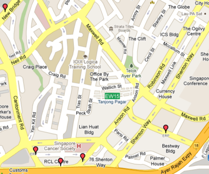
Figure 1: The map of Tanjong Pagar area, Singapore with the locations of the ERP gantries.

Fig. 2 shows the traffic flow on Anson Road, which is one of the roads that can be used to enter the Tanjong Pagar area, during the weekdays of August 2010 as well as the ERP rate. For the morning peak hours (roughly, from 7am to 10:30am), there are 3 noticeable peaks in the flow: at 7:55am, which is right before the ERP is effective, around 8:45am when the charge is maximum and at 10:00am, which is right after the ERP become inactive. From this consistent observation over all the weekdays of August 2010, it is reasonable to conclude that a significant portion of the motorists who regularly use this road intentionally adjust their schedule to avoid being charged.

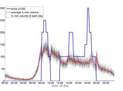
Figure 2: Traffic flow on Anson Road during the weekdays of August 2010.

Next we propose a model that explains the behavior observed in Fig. 2. Let ${\mathcal{T}}\subset{\mathbb{R}}_{\geq 0}$ denote the domain of $t$, $p(t),t\in{\mathcal{T}}$ denote the road price at time $t$, and $d(t),t\in{\mathcal{T}}$ denote the expected travel time from the motorist’s origin to destination, assuming that the motorist arrives at road ${\mathcal{R}}$ at time $t$. Consider the case where the travel cost is given by

$$J(t)=p(t)+J_{t}(t)+J_{d}(d(t)),$$ (2)

where $J_{t}:{\mathcal{T}}\to{\mathbb{R}}_{\geq 0}$ captures the cost of arriving earlier or later than the preferred arrival time $T$ and $J_{d}:{\mathbb{R}}_{\geq 0}\to{\mathbb{R}}_{\geq 0}$ captures the travel time factor of the travel cost.

As an initial step, we neglect the travel time factor and let

$$\begin{array}[]{rcl}J_{d}(d)&=&D,\forall d\geq 0\\ J_{t}(t)&=&\left\{\begin{array}[]{ll}b_{1}(T-t)&\hbox{if }t\leq T\\ b_{2}(t-T)&\hbox{otherwise}\end{array}\right.,\end{array}$$ (3)

where $D\geq 0$ is a constant and $b_{1},b_{2}\geq 0$ are the parameters that represent the amount of money the motorist is willing to pay to save a minute of early and late arrival respectively and may be different for different motorists. Assume that the preferred arrival time $T$ of each motorist is 8:45 am. Fig. 3 shows the optimal arrival time for each value of $b_{1}$ and $b_{2}$ for the case where $p(t)$ is the current price implemented on Anson road (cf. Fig. 2).

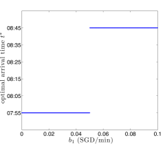
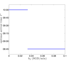
Figure 3: The $b$-$t^{*}$ relations, i.e., the optimal arrival time $t^{*}$ for each value of $b_{1}$ and $b_{2}$ for the case where $p(t)$ is the current price implemented on Anson road.

From Fig. 3, the optimal arrival time is only one of the followings: (a) 7:55am, which is right before the ERP is effective, (b) 8:45am, which is the preferred arrival time, (c) 10:00am, which is right after the ERP become inactive. This matches the observed behaviors of the motorists in Fig. 2. However, this optimal arrival time distribution is not efficient as there is a high concentration of demand only at 3 different times. Ideally, the optimal arrival times should be distributed equally among various time slots. In the next sections, we derive a pricing scheme that results in such an equally distributed optimal arrival times.

3 PRICING STRATEGIES

As a starting point, we consider the cost function in (2) with $J_{d}(d)$ and $J_{t}(t)$ as defined in (3). Assume that the preferred arrival time $T$ is the same for all motorists. Then, the optimal arrival time $t^{*}$ for each motorist with respect to the travel cost $J(t)$ only depends on the pricing scheme $p(t)$ and his/her time-money trade-off parameters $b_{1}$, $b_{2}$. For the simplicity of the presentation, we consider only motorists who prefer early over late arrival, i.e., $b_{2}\gg b_{1}$, and refer to $b_{1}$ simply as $b$ for the rest of this section. Similar results can be derived for motorists who prefer late over early arrival.

For a given pricing scheme $p$, we define a map $F_{p}:{\mathbb{R}}_{\geq 0}\to[0,T]$ that takes the time-money trade-off parameter and returns the maximum optimal arrival time as follows

$$F_{p}(b)=\max\left(\operatorname*{arg\,min}_{t}\big{(}p(t)+b(T-t)+D\big{)}\right).$$ (4)

Given a desired map $F:{\mathbb{R}}_{\geq 0}\to[0,T]$, in this section, we derive a pricing scheme $p$ such that $F_{p}=F$. We consider the case where $F$ is a monotonically increasing step function, e.g., as shown in Fig. 4. In this case, $F$ can be written as

$$F(b)=\left\{\begin{array}[]{ll}T_{i}&\hbox{if }B_{i}\leq b<B_{i+1},\forall i\in\{1,\ldots,N-1\}\\ T_{N}&\hbox{if }b\geq B_{N}\end{array}\right.,$$ (5)

where $N\in{\mathbb{N}}$, $0=B_{1}<B_{2}<\ldots<B_{N}$ and $0\leq T_{1}<T_{2}<\ldots<T_{N}=T$.

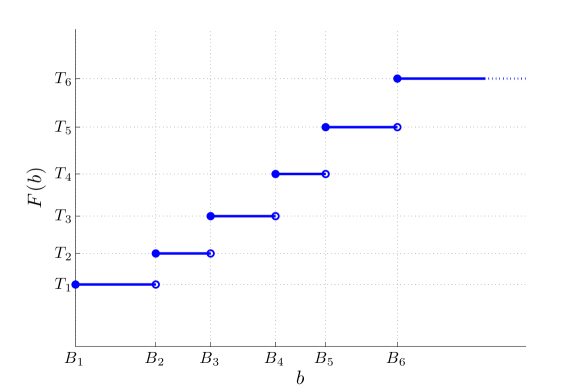
Figure 4: Example of a desired map $F$ for $N=6$.

Proposition 3.1

Consider the case where $p(t)$ is a step function. Define $p_{1},p_{2},\ldots,p_{N}$ such that

$$p(t)=\left\{\begin{array}[]{ll}p_{1}&\hbox{if }t\leq T_{1}\\ p_{i}&\hbox{if }T_{i-1}<t\leq T_{i},\forall i\in\{2,\ldots,N\}\end{array}\right.$$ (6)

Then, $F_{p}=F$ if

$$p_{i}=\sum_{k=2}^{i}B_{k}(T_{k}-T_{k-1})+p_{1},\forall i\in\{2,\ldots,N\}.$$ (7)

• From (4), (5) and (6), it can be checked that a necessary and sufficient condition for $F_{p}=F$ is that for each $i,j\in\{1,\ldots,N\}$,

  $$p_{i}+b(T-T_{i})\leq p_{j}+b(T-T_{j}),\forall b\in[B_{i},B_{i+1}).$$ (8)

  The case where $j=i$ is trivial so we only need to consider the case where $j\not=i$. Since $T_{j}>T_{i}$ and $B_{j}>B_{i}\geq 0$ for all $j>i$, condition (8) is satisfied if

  $$p_{i}\leq\left\{\begin{array}[]{ll}B_{i}(T_{i}-T_{j})+p_{j},&\forall j<i\\ B_{i+1}(T_{i}-T_{j})+p_{j},&\forall j>i\end{array}\right.$$ (9)

  First, consider the case where $j<i$. Since $B_{k}>B_{i},\forall k>i$, we get

  $$\sum_{k=j+1}^{i}B_{k}(T_{k}-T_{k-1})\leq\sum_{k=j+1}^{i}B_{i}(T_{k}-T_{k-1})=B_{i}(T_{i}-T_{j}).$$

  Adding $\sum_{k=2}^{j}B_{k}(T_{k}-T_{k-1})+p_{1}$ to both sides and using (7), we get

  $$p_{i} = \sum_{k=2}^{i}B_{k}(T_{k}-T_{k-1})+p_{1}$$

  $$\leq B_{i}(T_{i}-T_{j})+\sum_{k=2}^{j}B_{k}(T_{k}-T_{k-1})+p_{1}$$

  $$= B_{i}(T_{i}-T_{j})+p_{j}$$

  With similar reasoning, for the case where $j>i$, we have

  $$B_{i+1}(T_{j}-T_{i})=\sum_{k=i+1}^{j}B_{i+1}(T_{k}-T_{k-1})\leq\sum_{k=i+1}^{j}B_{k}(T_{k}-T_{k-1}).$$

  Adding $B_{i+1}(T_{i}-T_{j})+\sum_{k=2}^{i}B_{k}(T_{k}-T_{k-1})+p_{1}$ to both sides, we get

  $$p_{i} = \sum_{k=2}^{i}B_{k}(T_{k}-T_{k-1})+p_{1}$$

  $$\leq B_{i+1}(T_{i}-T_{j})+\sum_{k=2}^{j}B_{k}(T_{k}-T_{k-1})+p_{1}$$

  $$= B_{i+1}(T_{i}-T_{j})+p_{j}$$

  Hence, condition (9) is satisfied and we can conclude that $F_{p}=F$.

Example 3.1

Consider the case where $N=6$, $B_{i}=0.02(i-1)$, $T_{i}=T-10(N-i)$, $i\in\{1,\ldots,N\}$. With $p_{1}=0$, according to (7), we get $p_{2}=0.2$, $p_{3}=0.6$, $p_{4}=1.2$, $p_{5}=2$ and $p_{6}=3$. This pricing scheme as well as the one currently implemented are shown in Fig. 5.

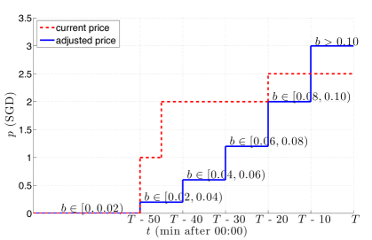
Figure 5: Example of the proposed pricing scheme. The range of $b$ associated with each price is also shown.

4 CASE STUDY OF SINGAPORE

Reconsider the motivational example in Section 2. Assume that $b$ has a Gaussian distribution with a certain mean $\mu_{b}$ and variance $\sigma_{b}$. The set of possible means and variances of b can be computed from historical data. For example, Fig. 6 shows possible distributions of $b$ based on the ratio between the average number of motorists at 7:55am and at 8:45am (cf. Fig. 2).

Using the distribution with mean $0.051$ (Fig. 6), the map $F$ can be computed such that the numbers of motorists at times $T_{1},\ldots,T_{N}$ are equal. An example of such $F$ for $N=6$, $T_{i}=T-10(N-i),i\in\{1,\ldots,N\}$ is shown in Fig. 7. The corresponding pricing scheme based on Eq (7) is shown in Fig. 8.

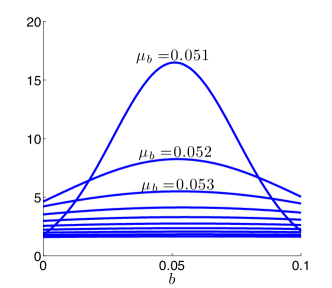
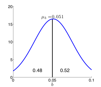
Figure 6: (left) Possible distributions of $b$. (right) Distribution of $b$ with mean $0.051$

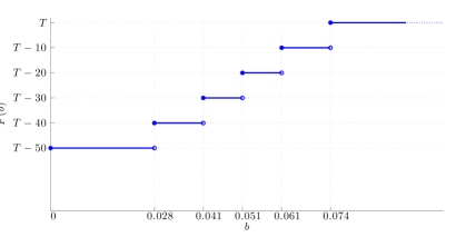
Figure 7: A map $F$ that leads to the equal number of motorists at times $T_{1},\ldots,T_{6}$, assuming that $b$ has a Gaussian distribution with mean 0.051.

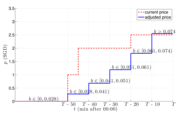
Figure 8: The corresponding pricing scheme based on the map $F$ provided in Fig. 7.

The current flow between 7:55am and 8:45am and the results from 10,000,000 Monte Carlo simulations based on the model in (1) with the cost function $J(t)$ defined in (2) and (3) are shown in Fig. 9. The actual arrival time is obtained by adding some Gaussian noise to the optimal arrival time $t^{*}$.

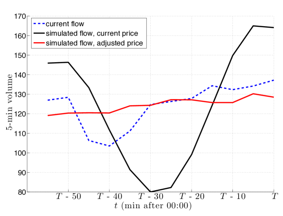
Figure 9: The current flow between 7:55am and 8:45am and the results obtained from 10,000,000 Monte Carlo simulations using the model in (1) with the current price and the adjusted price based on Eq (7).

5 CONCLUSIONS AND FUTURE WORK

We provided a case study of Singapore road network that shows that road pricing could significantly affect commuter trip timing behaviors. Based on this empirical evidence, we proposed a model that describes the commuter trip timing decisions. The analysis and simulation results showed that the proposed model reasonably matches the observed behaviors. In addition, we proposed a pricing scheme based on the proposed model in order to better spread peak travel and reduce traffic congestion. Simulation results showed that uniform distribution of arrival times among motorists who regularly use the road during the peak hours could be obtained.

Future work includes considering multiple roads and incorporating the route choice behavior in the model. We also plan to take into account stochasticity in the actual arrival time as the motorist may not arrive exactly at his/her optimal arrival time. In addition, we are interested in incorporating the travel time factor in the model. The average travel time for different origins and destinations as well as the portion of motorists with those origin and destination pairs can be estimated from the data obtained from all the taxi trips that went through a road of interest. We also plan to introduce stochasticity in the preferred arrival time $T$ (which depends, for example, on individuals’ work hours).

6 ACKNOWLEDGMENTS

The authors gratefully acknowledge Ketan Savla for the inspiring discussions and Land Transport Authority of Singapore for providing the data collected from the loop detectors installed on Anson road. This work is supported in whole or in part by the Singapore National Research Foundation (NRF) through the Singapore-MIT Alliance for Research and Technology (SMART) Center for Future Urban Mobility (FM).

References

- [Button and Verhoef(1998)] Button, K. J. and E. T. Verhoef, 1998: Road Pricing, Traffic Congestion and the Environment: Issues of Efficiency and Social Feasibility. Edward Elgar Pub.
- [Chin(1990)] Chin, A., 1990: Influences on commuter trip departure time decisions in Singapore. Transportation Research Part A: General, 24 (5), 321–333.
- [Como et al.(2011)Como, Savla, Acemoglu, Dahleh, and Frazzoli] Como, G., K. Savla, D. Acemoglu, M. A. Dahleh, and E. Frazzoli, 2011: Robust distributed routing in dynamical flow networks - part II: Strong resilience, equilibrium selection and cascaded failures. IEEE Transactions on Automatic Control, URL http://arxiv.org/abs/1103.4893, submitted.
- [Deakin et al.(1996)Deakin, Harvey, Pozdena, and Yarema] Deakin, E., G. Harvey, R. Pozdena, and G. Yarema, 1996: Transportation pricing strategies for California: An assessment of congestion, emissions, energy, and equity impacts. Tech. rep., The University of California.
- [Kurzhanskiy and Varaiya(2010)] Kurzhanskiy, A. A. and P. Varaiya, 2010: Active traffic management on road networks: a macroscopic approach. Philosophical Transactions of the Royal Society A: Mathematical, Physical and Engineering Science, 368 (1928), 4607–4626.
- [McFadden(1973)] McFadden, D., 1973: Conditional logit analysis of qualitative choice behavior. Frontiers in Econometrics, 105–142.
- [Menon(2000)] Menon, A. P. G., 2000: ERP in Singapore - a perspective one year on. Traffic Engineering and Control, 41 (2), 40–45.
- [Olszewski and Xie(2005)] Olszewski, P. and L. Xie, 2005: Modelling the effects of road pricing on traffic in Singapore. Transportation Research Part A: Policy and Practice, 39 (7-9), 755–772.
- [Orosz et al.(2010)Orosz, Wilson, and Stépán] Orosz, G., R. E. Wilson, and G. Stépán, 2010: Traffic jams: dynamics and control. Philosophical Transaction of the Royal Society A: Mathematical, Physical and Engineering Science, 368 (1928), 4455–4479.
- [Patriksson(1994)] Patriksson, M., 1994: The traffic assignment problem: models and methods. Topics in transportation, VSP.
- [Tsekeris and Voß(2009)] Tsekeris, T. and S. Voß, 2009: Design and evaluation of road pricing: state-of-the-art and methodological advances. NETNOMICS, 10, 5–52.
- [Wardrop(1952)] Wardrop, J. G., 1952: Some theoretical aspects of road traffic research. Proceedings of the Institution of Civil Engineers, Part II, 1 (3), 325–362.